Abstract
The conservation of biodiversity in intensively managed agricultural landscapes depends on the amount and spatial arrangement of cultivated and natural lands. Conservation incentives that create semi-natural grasslands may increase the biodiversity of beneficial insects and their associated ecosystem services, such as pollination and the regulation of insect pests, but the effectiveness of these incentives for insect conservation are poorly known, especially in North America. We studied the variation in species richness, composition, and functional-group abundances of bees and predatory beetles in conservation grasslands surrounded by intensively managed agriculture in Southwest Ohio, USA. Characteristics of grassland patches and surrounding land-cover types were used to predict insect species richness, composition, and functional-group abundance using linear models and multivariate ordinations. Bee species richness was positively influenced by forb cover and beetle richness was positively related to grass cover; both taxa had greater richness in grasslands surrounded by larger amounts of semi-natural land cover. Functional groups of bees and predatory beetles defined by body size and sociality varied in their abundance according to differences in plant composition of grassland patches, as well as the surrounding land-cover diversity. Intensive agriculture in the surrounding landscape acted as a filter to both bee and beetle species composition in conservation grasslands. Our results support the need for management incentives to consider landscape-level processes in the conservation of biodiversity and ecosystem services.
1. Introduction
Agricultural intensification has influenced biodiversity and ecosystem services in agricultural regions around the world [,]. At the local field scale, increased uses of crop monocultures, greater inputs of fertilizers and pesticides, and decreased within-field heterogeneity all may affect species diversity and composition and the provision of ecosystem services to agricultural productivity [,]. Increased field size also increases the isolation between production areas and the semi-natural and natural elements of the landscape that contribute to biodiversity and functional redundancy in ecosystem services [,]. Landscape-level intensification includes the loss of more natural forest or grassland habitat and decreases in field margins, filter strips, or grass waterways. Together, these local and landscape-level practices selectively filter species assemblages in a manner that depends on species variation in body size, dispersal ability, and habitat or diet specificity [,,]. Ecological processes may therefore interact at the local and landscape levels to influence farmland biodiversity at multiple spatial scales [,,].
Over the past several decades, farming systems in many regions have shifted from smaller fields with a more diverse array of crops to larger fields with few crop types and little surrounding natural or extensively managed lands [,,]. Land-use intensification may reduce the abundance and diversity of plants, birds, and predatory or pollinating insects [,,]. Conservation programs, such as Agri-Environmental Schemes in Europe and the Conservation Reserve Program in the US, provide economic incentives to convert marginal cropland into managed, semi-natural habitat that support game animals and help prevent topsoil erosion []. The benefits of these programs to biodiversity are still poorly known, however, since they may vary among taxa or functional groups and depend on the extent of their implementation in the larger landscape [,,,].
Natural and semi-natural habitats in agricultural landscapes support a greater diversity of pollinating and predatory insects that provide ecosystem services in both semi-natural and cultivated areas (e.g., [,,]). These semi-natural habitats provide resources such as nectar and pollen from a diversity of flowering plants, a variety of prey or hosts, and overwintering and nesting habitat for pollinators and predatory insects (e.g., [,,]). Fragmentation and loss of semi-natural habitat impact plants species richness and the resources that plants provide for beneficial insects within agricultural landscapes [,].
Natural and semi-natural patches often provide stable resources that support diverse assemblages of plants necessary to sustain resident populations of pollinators and predatory insects [,,]. The turnover in composition of insect species among natural and semi-natural patches may lead to shifts in community interactions and ecosystem functions within agricultural landscapes []. Ecosystem functioning is increased when contrasting resources are used by a complementary set of organisms, because different species occupy dissimilar habitats []. Habitat loss and changes in land use/land cover may cause declines in the biodiversity of pollinators and natural enemies, depending on life history traits of plant-dependent organisms [,].
Agricultural landscapes of southwest Ohio, USA, are embedded within the larger “corn belt” of the upper Midwestern US, a region that has undergone substantial agricultural intensification resulting in large field sizes and low crop diversity [,]. Although few natural forest remnants and grasslands remain, these natural remnants along with conservation practices, such as riparian buffers, perennial field margins, and grass filter strips, may support larger numbers of natural enemies and pollinating insects than are found in arable crop fields alone [,,]. Larger tracts of semi-natural habitat are established on marginal agricultural lands and planted with native perennial herbaceous vegetation under temporary lease agreements with the US Department of Agriculture Conservation Reserve Program (CRP) or long-term grassland restoration supported by Habitat Enhancement Grants (HEG) from US Fish and Wildlife Service (USFWS), the latter with matching funds from local conservation organizations. These grants provide subsidies to farmers for planting semi-natural habitats in lieu of crops [,]. Conservation grasslands are known to provide essential ecosystem services such as erosion control and wildlife habitat [], but fewer studies have examined their roles in supporting beneficial insects [,].
We studied the species diversity, composition, and abundance of functional groups of bees and predatory beetles, in habitat patches of conservation grasslands embedded within intensive agricultural landscapes in SW Ohio. All grasslands were established on privately owned farmlands through conservation incentives, and differed in the size and time since planting. Limited data exist on the amounts of natural and semi-natural habitat or the availability of floral resources needed in the landscape to support diverse assemblages of pollinators and predators in agricultural landscapes of Midwestern North America [,]. In conservation grasslands, other factors that could influence the biodiversity of bees and predatory beetles include patch area, time since planting (age), and plant community composition. The colonization and persistence of insect predators and pollinators in grassland patches may also depend on the diversity and relative amounts of land use/land cover in the surrounding landscape [,]. Insects with a smaller body size or lower dispersal ability often show stronger effects of suitable habitat area than do large or generalist species [], but small-bodied species or poor dispersers may be impeded by colonization of suitable habitats if the surrounding landscape matrix is highly unsuitable [,].
We hypothesized that the abundances of bees and predatory beetles would respond to habitat and landscape characteristics differently according to functional groups based on body size, dispersal ability, and sociality. Further, we hypothesized that variation in species occurrence and abundance within functional groups would translate into community-level differences in species richness and composition among conservation grasslands. We predicted that the larger, older grassland patches with greater floral resources would have higher species richness and functional-group abundances of bees and beetles. At the landscape level, we predicted that grassland patches with greater amounts of surrounding grassland and forest habitats would also support higher bee and beetle species richness and functional-group abundance. Lastly we predicted functional groups of bees and beetles with smaller body size or lower dispersal ability would be more strongly influenced by surrounding landscape than patch-level characteristics for conservation grasslands surrounded by high amounts of intensive agriculture.
2. Methods
2.1. Study Region
The study was conducted during summer 2009 in 10 conservation grasslands established through temporary lease agreements with support from the USDA-CRP or long-term restoration supported by the USFWS-HEG. Patches were scattered in a 310 km2 agricultural region within Butler and Preble Counties, Ohio, USA. Nearest-neighbor distances between adjacent patches ranged from 2 to 10 km. In 2009, approximately 51% of Butler County was active cropland, 23% forests, 12% urban, and 11% pasture. In Preble County active cropland was approximately 67%, 17% forest, 8% pasture, and 6% urban [].
Study patches ranged in size from 1.2 to 17.8 ha, and were planted in native warm-season grasses and forbs. Time since planting ranged from 1 to 13 yr, and most areas were cultivated prior to planting perennial grasses and forbs. All sites were planted with a similar mix of grasses and forbs, but grasslands varied in species dominance, diversity, and composition of the established plant community (Table A1). Dominant grasses included big blue stem (Andropogon gerardii), little blue stem (Schizachyrium scoparium), switchgrass (Panicum virgatum), Indian grass (Sorghastrum nutans), and side oats grama (Bouteloua curtipendula). A variety of forbs were present, including partridge pea (Cassia fasiculata), Illinois bundleflower (Desmanthus illinoensis), coneflower (Echinacea purpurea), and Maximilian sunflower (Helianthus maximiliani). The land use/land cover types (hereafter “land cover”) surrounding the conservation grassland were dominated by row-crop agriculture (mostly corn and soybeans), but also included woodlots and riparian forest, pasture and hayfields, and suburban areas.
2.2. Insect Sampling
All grasslands were sampled during 2-week periods twice during the summer of 2009: 26 May–8 June and 27 July–10 August (hereafter referred to as June and August samples). Five sites were randomly selected to sample during the first week and five during the second week in each of the two sample periods. Random site selection was constrained to include small and large patches in each week of the sampling window. The order of sampling of each site remained the same for both sampling periods.
Combination flight intercept and pan traps were used to sample aerial insects (modified after []). Flight intercept traps were constructed of yellow buckets (7.6 L; 29 cm diam. × 21 cm tall) with a pair of perpendicular Lexan™ panes inserted into the bucket and extending 41 cm from the top (Figure 1). Traps captured both pollinators and weak-flying insects, with the former attracted to the yellow buckets while the latter were intercepted by the extended panes. Buckets were partially filled with water and elevated on 1-m platforms, which were above the plant canopy during the first sampling period (Figure 1) and approximately level with the canopy during the second sampling period. A few drops of detergent were added to the bucket to reduce surface tension. Pitfall traps were used to sample ground-dwelling insect arthropods. Traps were plastic cups (75 mm diam × 80 mm deep) placed flush with the ground surface and at least 1 m from each aerial trap. Ethylene glycol was added to each pitfall trap as a killing agent.
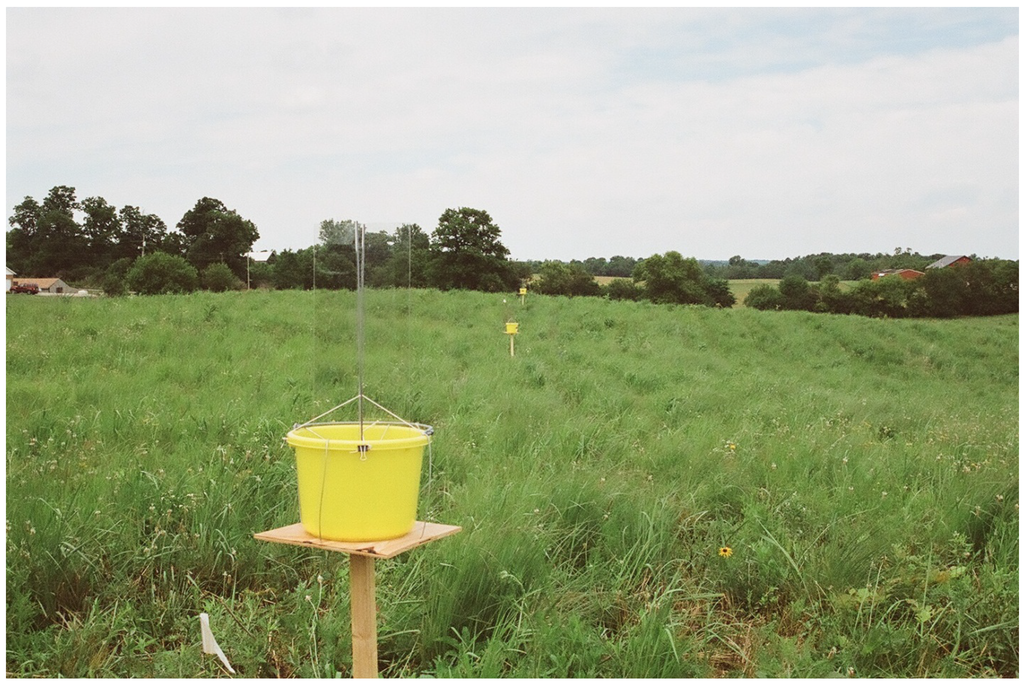
Figure 1.
Combined flight-intercept and pan trap used to sample bees and beetles along transects within 10 conservation grasslands in agricultural landscapes of southwestern Ohio, USA. Traps were spaced at 25-m intervals, and a pitfall trap was located within 1 m of each flight trap to sample ground-dwelling insects.
The traps were arranged in transects through the center axis of the long dimension of each grassland patch. The number of traps in each patch was scaled to the logarithm of the patch area, ranging from 5 traps at the smallest site to 10 traps at the largest site. Trap spacing was 25 m at all sites. The flight-intercept/pan traps and the pitfall traps were positioned in the same locations in the early and late season sampling periods. At the end of each 2-wk sample period, trap contents were poured through No-see-um netting (Nicamaka™) then washed with 70% ethanol into a Nalgene™ bottle for temporary storage. In the laboratory, bees (Apoidea) were sorted and identified to taxonomic species [,]. Focal families of Coleoptera (predatory beetles) were also sorted and identified to species [,]. Some beetles identified were parasitoids (Meloidae and Ripiphoridae, and Lebiinae subfamily), but were considered predatory beetles in this study. Complete species lists of bees and predatory beetles recorded in this study are provided in Table A3 and Table A4.
2.3. Vegetation Sampling
Plant sampling was conducted twice during the summer (15 June and 20 August) to capture phenological changes in vegetation cover and floral resources during the early and late sampling periods. Vegetation cover was recorded in a pair of 10-m2 circular quadrats located 3 m from each side of the trap and perpendicular to the transect line. Estimated cover was recorded for each plant species as 0%, 1%, 5%, 10%, 25%, 50%, 75% or 100%. The total number of flowering forb stems was also recorded by species. Means were calculated across quadrats within each site for flowering stem density, total plant cover, and cover values by C3 and C4 grasses, forbs, sedges and woody plants.
2.4. Landscape Variables
Digital Orthophoto Quadrangles, (0.15 m resolution for Butler County, 3 m resolution for Preble County) and Geographic Information Systems, ArcGIS version 9.3.1 [], were used to quantify the area and diversity of surrounding land cover types. On-screen digitizing of land cover was implemented within circular windows of eight varying radii (130, 185, 260, 370, 525, 740 m) from the central point of the transect (Figure 2), doubling the area sampled with each larger radius ranging from 5.3 ha (130 m) to 172 ha (740 m). The land cover types were analyzed in the entire area of each successively larger circle, rather than the areas defined by concentric rings. Thus, for the larger conservation grasslands (10–18 ha), the area of the patch itself could constitute most or all of the area within the two smallest circles but rapidly drops below 10% of the land area for larger circles. These radial distances and corresponding areas were chosen to reflect differential dispersal distances of the insect taxa under investigation [,] and to reduce overlap from adjacent habitats []. Land cover was classified as: (1) semi-natural grassland; (2) intensive agriculture; (3) extensive agriculture; (4) forest; (5) low-density residential; (6) high-density residential; and (7) water/wetland. Intensive agriculture was characterized by cultivated crops of corn, soybeans, or wheat, whereas extensive agriculture was hay fields or pastures. The Shannon-Weiner diversity of land cover types was also calculated within each radius using number and proportional area of each land cover type. Site visits were conducted to ground-truth land cover types classified from aerial imagery (Table A2).
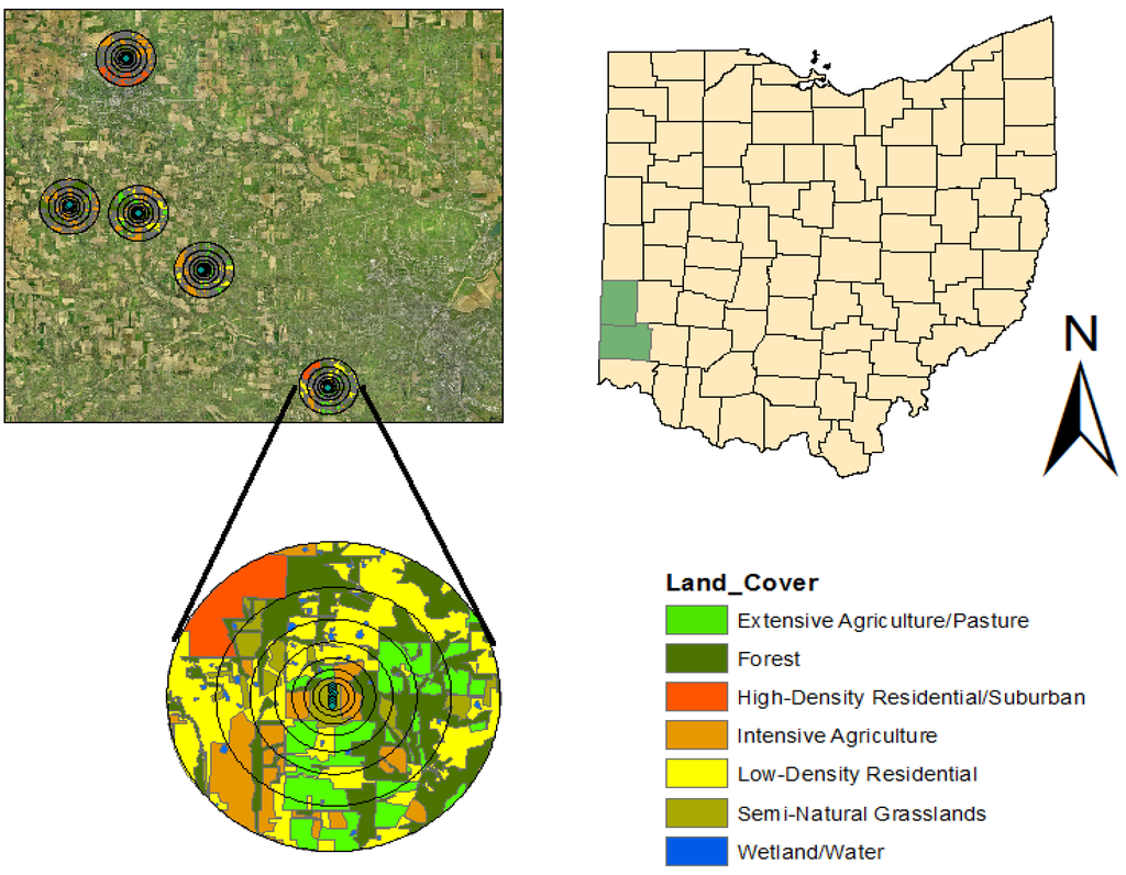
Figure 2.
Methods used to quantify land cover types around conservation grasslands. Aerial digital orthophotos were used to delineate seven different land cover types within multiple radii from the center of the sample transects within each grassland patches. Subsets of 5 of the 10 grasslands are shown from one of the two counties where the study was conducted in southwest Ohio, USA (green polygons in Ohio map).
2.5. Functional Groups of Bees and Beetles
Functional groups were defined for bees and beetles based on body size, vagility, and sociality. Bees were grouped according to the intertegular (IT) span between wing bases, which has been shown to be a good estimator of flight distances []. The median value of the IT span for all the species recorded in the study was used to classify bees as large (>2.5 mm) or small (<2.5 mm) species. Each species was also classified as social or solitary []. Bee abundances were later analyzed separately for large-solitary, large-social, small-solitary, and small-social functional groups. Beetles were placed into functional groups based on the median body length of all beetle species recorded (>5.5 mm large, <5.5 mm small) and wing type (brachypterous or macropterous) []. After dividing beetles into these two functional groups, however, we found that the two groups separated in a similar fashion such that site abundance numbers based on the two functional groups were nearly identical, so that the results of the statistical analysis were similar for large and macropterus beetles and for small and brachypterous beetles. We therefore report only those results from two functional groups of beetles based on body size alone.
2.6. Statistical Analysis
We analyzed the species richness, composition, and functional group abundances of bees and beetles separately by early and late season (June and August) because there was substantial turnover in species composition between seasons for both taxa. The plant species composition and flower availability also shifted between early and late season; cover of C3 grasses was greater in June than in August while C4 grass cover increased from early to late seasons. We therefore expected that insect communities would respond to these changes in patch-level resources.
Two sets of predictor variables were evaluated in multiple regression models of bee and beetle species richness and functional-group abundances. Predictor variables for each grassland patch included area (ha), age (yr), flower density (no∙m−2), plant species richness, and mean total plant cover, and mean cover of C3 grasses, C4 grasses, and forbs. Area, age and flower density were log-transformed prior to analysis. The area of each land cover type was converted into a proportion of the total areas within each radius. Proportional areas of intensive agriculture (row crops), extensive agriculture (pasture and hay), semi-natural grasslands, and forest were included as predictor variables in regression models; other land-cover types comprised a much smaller fraction of the total land cover. The Shannon diversity of all land-cover types was also screened as predictor variable. Counts of bee or beetle species richness and functional-group abundance were large enough to treat these measures as continuous Gaussian responses in multiple linear regressions against patch and landscape predictor variables. Regressions were conducted using the glm function in the base package of the R programming language version 3.02 []. Richness and abundance were log-transformed prior to analysis. A separate set of regressions were conducted using patch-level and land-cover variables to reduce the number of candidate predictor variables of each category, and to determine the best-fitting land-cover models among the eight radial distances. The patch- and landscape-level variables were then combined into a single regression model and a second round of model selection was conducted among these candidate predictor variables. Prior to model selection, we screened predictor variables that were highly correlated (Pearson r > 0.60) and did not include them in the same model; in these cases, a separate model selection was conducted involving each variable to determine which was more important to the overall model fit. During model selection, we also checked for collinearity by excluding combinations of variables that had a variance inflation factor > 4. The best-fitting model for each response variable was selected using the bias-corrected Akaike Information Criteria (AICc; []) containing both patch and landscape variables. The model residuals were also used to assess model fit. A likelihood ratio test was used to determine whether the best-fitting model explained a significant amount of the variation in species richness or functional-group abundance compared to the null model that included only the intercept.
To assess how patch- and landscape-level variables influenced the variation in species composition among patches, we conducted ordinations using distance-based redundancy analysis (dbRDA) with Bray-Curtis dissimilarity []. The method of dbRDA is a constrained ordination technique designed to test hypotheses on the roles of experimental factors or environmental variables on community composition [,]. The best fitting statistical model contained patch and landscape variables that had the lowest AICc, and p-values were obtained under random permutations (999 permutations). Analysis of dissimilarity was conducted using the vegdist function in the vegan package of R [], and dbRDA was conducted with a user-written function in R (M. Anderson, personal communication). Ordination plots were constructed for the results of the dbRDA using the unweighted site scores (first and second eigenvectors) and biplot projections of the best-fitting environmental variables representing the correlation with each ordination axis. The combined effect of the environmental variables can also be expressed as a percentage contribution of the overall variation in species dissimilarity across sites [].
3. Results
A total of 2672 bees representing 48 species were captured in flight intercept traps across both sampling periods (Table A3). The two sampling periods were comparable, with 1290 individuals of 36 species recorded in June and 1382 bees representing 37 species captured in August. A total of 3276 beetles representing 143 species were captured in flight-intercept and pitfall traps across both sampling periods (Table A4). Approximately twice as many beetles were found during the first sampling period compared to the second, with 2165 beetles of 115 species captured in June and 1111 beetles of 85 species in August. The Chao species estimator using species abundance data estimated bee species richness to be 58.1 species and beetle species richness at 175.7 species, with observed totals corresponding to 83% of the estimated bee richness and 81% of the estimated beetle richness.
3.1. Species Richness
Mean bee species richness in the sampled grasslands was 15.6 and 15.2 in June and August, respectively (range: 11 to 20 species). The best fitting model for bee species richness in June included positive effects of both forb cover at the patch level and the proportion of semi-natural grassland and forest habitat (within 525 m of the focal patch) in the surrounding landscape (Figure 3a; Table 1). The best fitting model for bee species richness in August included a negative effect of C3 grass cover and, although the model had a slightly higher AICc compared to the null (ΔAICc = 0.2), the likelihood ratio test shows the model to be a better fit than the null model (p = 0.04, Figure 4a; Table 1).
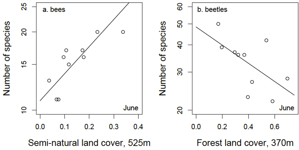
Figure 3.
(a) Relationship between bee species richness in 10 conservation grasslands during June and the proportion of semi-natural land cover within 525 m surrounding grassland patches; (b) Relationship between beetle species richness and amount of forest land cover within 370 m surrounding grassland patches.

Table 1.
Summary of regression results for the effects of vegetation composition and surrounding land cover on the species richness of bees and predatory beetles in 10 conservation grasslands. Standardized regression coefficients are shown. The P-value is the likelihood ratio test of the best-fitting model compared to the null model. Response variables with two sets of AICc and P-values are competing models.
| Response | Model Variables | Coefficient | AICc | ΔAICc | Deviance | P |
|---|---|---|---|---|---|---|
| Bee richness | Forb cover | +0.43 | −8.4 | 10.7 | 0.021 | <0.0001 |
| June | Semi-natural 525 m | +1.01 | ||||
| Forest 525 m | +0.51 | |||||
| Null | 2.3 | 0.414 | ||||
| Bee richness | C3 grass cover | −0.58 | −9.9 | 0.2 | 0.082 | 0.0400 |
| August | Null | −9.7 | 0.123 | |||
| Beetle richness | Forest 370 m | −0.60 | 6.5 | 0.3 | 0.412 | 0.0300 |
| June | Null | 6.7 | 0.649 | |||
| Beetle richness | Shannon diversity 525 m | +0.62 | −11.2 | 15.2 | 0.039 | <0.0001 |
| August | Semi-natural 260 m | +0.53 | ||||
| Null | 4.0 | 0.494 |
Mean beetle species richness in the sampled grasslands was 34 and 25.4 in June and August, respectively (range: 19 to 50 species). The amount of forest cover in the surrounding landscape (within a 370 m radius) had a negative effect on the number of beetle species captured in June (Figure 3b). This best fitting model was statistically significant but only a slight improvement over the null (Table 1). The best fitting model for August beetle species richness included a positive effect of land cover diversity within a 525 m radius and a positive effect of the amount of semi-natural habitat within a 260 m radius (Figure 4b; Table 1).
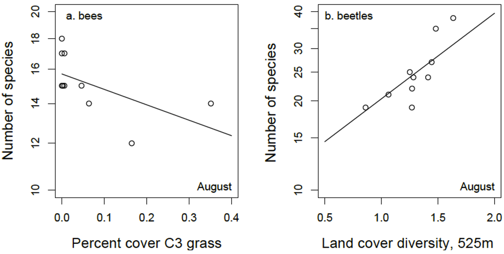
Figure 4.
(a) Relationship between bee species richness in 10 conservation grasslands during August and the proportional of C3 grasses within grassland patches; (b) Relationship between beetle species richness and land cover diversity in a 525 m radius surrounding grassland patches.
3.2. Bee Functional Groups
During the early season, all bee functional groups were best described by landscape-level variables. The best model for large (IT span > 2.5 mm), social bees included a negative effect of the amount of intensive agriculture within 525 m of focal patches (Figure 5a), while the abundance of large, solitary bees was best explained by the amount of semi-natural grassland in the landscape at the 260 m radius scale. Competing models for large bees included a positive effect of the amount of semi-natural habitat at the 740 m radius scale for large, social bees and a positive effect of land cover diversity within 740 m of focal patches for large, solitary bees (Table 2). For small (IT span < 2.5 mm), social bees, the best model included a negative effect of intensive agriculture within a 740 m radius landscape (Figure 5b). The second best model for small, social bees included a positive effect of the amount of semi-natural grassland within a 185 m radius landscape. For small, solitary bee abundance, the best model included a positive effect of the amount of semi-natural habitat within 370 m of focal patches (Figure 5c).
Results of functional-group abundance during the late season differed from the early season. Late season functional-group bee abundance showed a response to both patch-level and landscape-level variables. Specifically, late season large, solitary and small, social bee abundance best models included effects of the proportion of forbs at the local scale (Table 2). The best fitting model for large, solitary bees also included a negative effect of extensive agriculture cover within 525 m of focal patches. For small, social bee abundance there were two competing models. The best fitting model for small, social bee abundance, with 61% of the weight of evidence, included a positive effect of land cover diversity within the 525 m radius landscape. A competing model for small, social bees, with 15% of the weight of evidence included a positive effect of land cover diversity within the 525 m radius landscape and a positive effect of the proportion of forbs at the local scale. No landscape- or patch-level predictors significantly explained the variation in large, social bee abundance during the late season, and the null model was the best fitting model (Table 2). Finally, for small, solitary bee abundance during the late season, the best model included a positive effect of forest cover at the 740 m landscape scale.
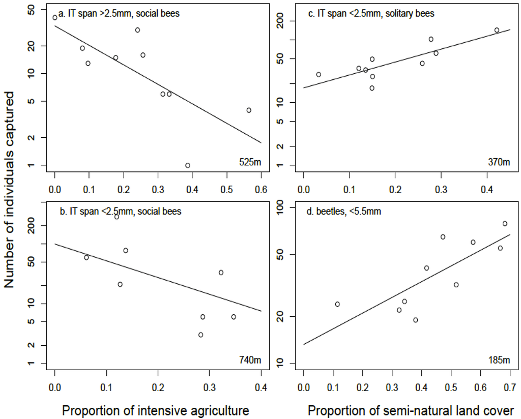
Figure 5.
Relationships between functional group abundances of insects and the proportion of intensive agriculture and semi-natural land cover in the landscape surrounding 10 conservation grasslands (a) large, social bees with intertegular (IT) span > 2.5 mm (b) small, social bees with IT span < 2.5 mm (c) small, solitary bees with IT span <2.5 mm (d) small beetles with body size < 5.5 mm in length.
Table 2.
Summary of regression results for the effects of vegetation composition and surrounding land cover on the abundance of bees in 10 conservation grasslands. Standardized regression coefficients are shown. The P-value is the likelihood ratio test of the best-fitting model compared to the null model. Response variables with two sets of AICc and P-values are competing models.
| Response | Predictor Variables | Coefficient | AICc | ΔAICc | Deviance | P |
|---|---|---|---|---|---|---|
| June | ||||||
| Social, large | 1. Intensive agriculture 525 m | −0.74 | 30.99 | 3.8 | 4.78 | 0.002 |
| 2. Semi-natural 740 m | +0.67 | 33.1 | 1.7 | 5.90 | 0.01 | |
| Null | 34.79 | 10.73 | ||||
| Solitary, large | 1. Semi-natural 260 m | +0.70 | 38.8 | 2.4 | 10.4 | 0.006 |
| 2. Shannon diversity 740 m | +0.68 | 39.1 | 1.3 | 10.8 | 0.008 | |
| Null | 41.2 | 20.2 | ||||
| Social, small | 1. Intensive agriculture 740 m | −0.71 | 38.9 | 2.8 | 10.6 | 0.004 |
| 2. Semi-natural 185 m | +0.64 | 40.7 | 1.0 | 12.6 | 0.018 | |
| Null | 41.7 | 21.5 | ||||
| Solitary, small | 1. Semi-natural 370 m | +0.82 | 17.2 | 7.0 | 1.20 | <0.0001 |
| Null | 24.2 | 3.72 | ||||
| August | ||||||
| Social, large | Null* | 26.8 | 1.3 | 4.83 | ||
| 1. Flower density | +0.51 | 28.1 | 3.59 | 0.097 | ||
| Solitary, large | 1. Extensive agriculture 525 m | −0.56 | 19.4 | 7.7 | 0.82 | <0.0001 |
| Forb cover | −0.61 | |||||
| Null | 27.1 | 4.99 | ||||
| Social, small | 1. Shannon diversity 525 m | +0.79 | 24.9 | 5.5 | 2.59 | 0.0003 |
| 2. Forb cover | +0.36 | 27.6 | 2.8 | 1.29 | 0.13 | |
| Shannon diversity 525 m | +0.64 | |||||
| Null | 30.4 | 6.91 | ||||
| Solitary, small | 1. Forest 740 m | +0.61 | 14.5 | 0.5 | 0.92 | 0.028 |
| Null | 15.0 | 1.48 | ||||
* The null model has the lowest AICc, with flower density as a competing model.
3.3. Beetle Functional Groups
In the early season, the null model was the best fitting model for large beetle abundance (Table 3). Three candidate models best described the variation in small beetle abundance in sampled grasslands during the early season. A positive effect of C4 grass cover had 20% of the weight of evidence, the null model was the second best fit, with 19% of the weight of evidence, and the third competing model, with 14% of the weight of evidence, included positive effects of both C4 grass cover at the patch level and land cover diversity at the 370 m landscape scale (Table 3).
The best-fitting regression models for late season beetle abundance included both patch-level and landscape-level factors (Table 3). Patch area showed a positive relationship with small beetle abundance in the best fitting model, with 36% of the weight of evidence, while the second best model, with 29% of the weight of evidence included a positive effect of semi-natural cover within 185 m radius surrounding the sampling plot (Figure 5d). Similarly, two top models were identified for large beetle abundance in the late season. First, with 53% of the weight of evidence, the best fitting model included a positive effect of the amount of C3 grass cover at the patch level and a negative effect of the amount of forest in a landscape at the 370 m radius. The second best model, with 21% of the weight of evidence, included a positive effect of land cover diversity at the 525 m scale.
Table 3.
Summary of regression results for the effects of vegetation composition and surrounding land cover on the abundance of large and small bodied beetles in 10 conservation grasslands. Standardized regression coefficients are shown. The P-value is the likelihood ratio test of the best-fitting model compared to the null model. Response variables with two sets of AICc and p-values are competing models.
| Response Variable | Predictor Variables | Coefficient | AICc | ΔAICc | Deviance | P |
|---|---|---|---|---|---|---|
| June | ||||||
| Large | Null * | 21.8 | 1.3 | 2.93 | ||
| (>5.5 mm) | 1. C3 grass cover | +0.51 | 23.2 | 2.18 | 0.097 | |
| Small (<5.5 mm) | 1. C4 grass cover | +0.60 | 27.4 | 0.1 | 3.35 | 0.036 |
| 2. C4 grass cover | +1.08 | 1.98 | ||||
| Shannon diversity 370 m | +0.70 | 28.2 | −0.1 | 0.004 | ||
| Null | 27.5 | 5.18 | ||||
| August | ||||||
| Beetles (>5.5 mm) | 1. C3 grass cover | +0.74 | 20.7 | 4.8 | 0.94 | <0.0001 |
| Forest 370 m | −0.65 | |||||
| 2. Shannon diversity 525 m | +0.72 | 22.5 | 3.0 | 2.04 | 0.003 | |
| Null | 25.5 | 4.24 | ||||
| Small (<5.5 mm) | 1. Patch area | +0.79 | 14.1 | 5.6 | 0.88 | 0.0002 |
| 2. Semi-natural 185 m | +0.78 | 14.6 | 5.1 | 0.92 | 0.0004 | |
| Null | 19.7 | 2.37 | ||||
* The null model has the lowest AICc with C3 grass cover as a competing model.
3.4. Community Composition
All best-fitting models for bee and beetle community composition, with one exception, included both a patch-level and a landscape-level predictor variable. Variation in bee community composition among the conservation grasslands during early summer was best explained by the amount of intensive agriculture within 525 m of the surrounding landscape, and by the density of flowers in conservation grasslands (Table 4; Figure 6a). Bee community composition during late summer was characterized best by the diversity of land cover types within 370 m and by the proportion of forb cover at the patch level (Figure 6b). The beetle community of the conservation grasslands responded more strongly to patch-level variables compared to the bee community. During the early season, the variation in beetle community composition was best explained by the amount of intensive agriculture in the landscape, at the 740 m radius scale, and by proportional forb cover within grassland patches (Figure 6c). Finally, beetle community composition during the late season was most influenced by grassland patch area and by the proportional cover of C3 grasses (Figure 6d).
Table 4.
Summary of ordinations using distance-based redundancy analysis on the community composition of bees and predatory beetles. The pseudo F-statistic and p-value are based on 999 permutations of the species by sample matrix.
| Response | Predictor Variables | AICc | Pseudo F | P | R2 |
|---|---|---|---|---|---|
| Bees, June | Number flowers | −17.69 | 1.95 | 0.015 | 0.358 |
| Intensive ag 525 m | |||||
| Bees, August | Forb cover Shannon diversity 370 m | −20.38 | 1.70 | 0.038 | 0.327 |
| Beetles, June | Forb cover | −13.51 | 1.58 | 0.046 | 0.311 |
| Intensive ag 740 m | |||||
| Beetles, August | Patch area | −13.47 | 1.56 | 0.028 | 0.308 |
| C3 grass cover |
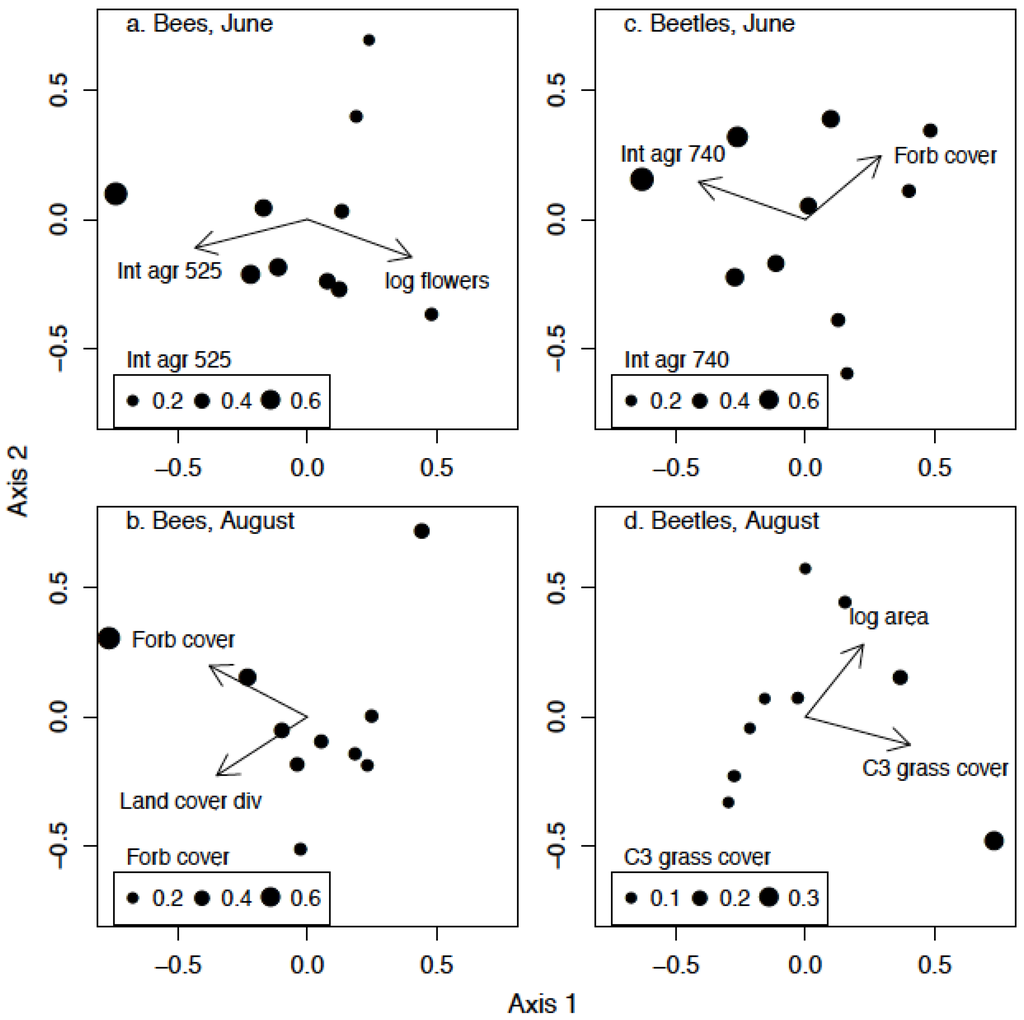
Figure 6.
Multivariate ordinations of bee and beetle community composition across the 10 conservation grasslands using distance-based redundancy analysis and Bray-Curtis dissimilarity. Symbols indicate site scores of grassland patches, and are sized proportional to the value of the most important predictor variable. Arrows are biplot correlations of the significant predictor variables. (a) bees in June (b) bees in August (c) beetles in June (d) beetles in August.
5. Discussion
Conservation of biodiversity in agricultural landscapes depends on large-scale patterns of land cover, patch-level characteristics and management actions, and the variation in species responses to habitat and resource availability at these multiple scales. Our study represents one of the first in North America to concurrently evaluate local and landscape-level factors potentially impacting the effectiveness of conservation grasslands for beneficial arthropods in agricultural landscapes. Our results highlight the importance of considering a landscape approach in planning of conservation grassland programs to ensure a sufficient amount of grassland habitat in a landscape. Since the size of semi-natural habitats is often limited to marginal production areas, the most feasible way to achieve this goal may be to provide incentives to increase the number of semi-natural habitat patches. Specifically, two key findings drive this management recommendation. First, all richness and abundance response variables with the exception of large beetles showed a positive response to the amount of semi-natural grassland cover in the landscape during at least one of the collection seasons. Second, we found a high degree of turnover in species composition of bees and predatory beetles among conservation grasslands along land-cover gradients of intensive agriculture and semi-natural grassland. These shifts in species composition across land-cover gradients were also accompanied by changes in functional group abundances of bees and beetles. Although our study did not determine how these changes translated into ecosystems services (pollination and pest control), other studies have suggested that large amounts of spatial variation in species composition across agricultural landscapes can provide insurance in ecosystem services to local disturbances or the loss of individual species [,].
The amount of semi-natural grassland cover in the surrounding landscape showed the strongest relationships with beetle and bee diversity, but our results indicate that the amounts of forest cover and intensive agriculture are also important to biodiversity conservation in agricultural landscapes. Species diversity and community composition have been linked to particular ecosystem services such as pollination services and biological control [,,]. In our study, forest cover variables were included in best models for both bee and beetle richness and intensive agriculture cover variables were included in best models for both bee and beetle community composition. Although overall insect species richness and abundance responses to intensive agriculture cover in the landscape were largely negative, there were clearly insect species assemblages in some grassland patches that were positively associated with nearby agricultural fields (Figure 6a,c).
Variation in the abundance of key ecosystem service providers has been shown to have the greatest impact on ecosystem service provisioning []. We found that variation in the abundance of both large and small social bees, which are known play a critical role in the seed and fruit set of many crop species [] was influenced by surrounding semi-natural grassland and intensive agriculture land cover. The bee assemblage associated with intensive agricultural cover was characterized by lower numbers of three very important pollinator groups: bumblebees, squash bees and honeybees. More specifically, of the 91 Bombus spp., 60 Apis mellifera and 21 Melissodes spp. collected in June, only 12, 5, and 1 bees, respectively, were from the 4 sites with >30% intensive agriculture cover within 525 m radius. Bee pollination services by wild bees and the honey bee Apis mellifera, specifically, are of great interest in the study area as new findings reveal a 6% increase in soybean yield with wild bee pollinators and an additional 18% increase in soybean yield with added honey bee colonies []. Fewer rare bees were also found in these grasslands, with only 7 of the 30 rare species (i.e., those with fewer than 4 occurrences) collected. Given the large foraging ranges of honeybees and bumblebees [] it may be surprising that lower numbers of these species are driving the association with intensive agriculture at this relatively small scale, but these findings are supported by a recent study that also found a negative response of large-bodied bees to agricultural land cover at a similar scale (300 m radius) [].
Greater amounts of surrounding land-cover diversity, as measured by the Shannon index, had positive effects on the responses of bee and beetle communities. Beetles generally showed positive effects of land-cover diversity (Table 1 and Table 3), possibly reflecting landscape complementarity [] in the use of pulsed prey resources in agricultural habitats [,] and the use of alternative prey, floral resources, or overwintering sites in semi-natural habitats [,]. Bees also showed a positive response to land-cover diversity, with large, solitary and small, social bee functional groups responding to two different scales of land-cover diversity.
We stress the importance of a landscape approach to conservation in agricultural lands, but our study supports other works showing that local habitat management is also important for effective biodiversity conservation [,]. All conservation grasslands in the reserve programs are initially planted with a similar mix of forbs and grasses, but post-planting management regime and time since establishment affect the trajectory of each vegetation class so that grassland plant community composition was highly variable in our study (Table A1). Not surprisingly, bees showed a stronger response than beetles to flower density and forb cover. The proportion of grassland covered by forbs was an important predictor variable for bee richness, abundance within some functional groups, and community composition across both seasons; however floral density was only included in best models for bee community composition during the early season. This difference may reflect the quality of the floral resources that are available in early versus late summer, as higher quality flowers such as bee balm Monarda spp. and purple prairie clover Dalea purpurea are typical of the early season and the lesser quality composite flowers characterized the late-summer grassland flower community.
The variation in the relative amounts of cool-season (C3) and warm-season (C4) grass cover among grassland patches was most associated with variation in the abundance of functional groups of beetles. Sites with greater cover of C3 grasses had a patchy, more open canopy structure, and those dominated by C4 grass cover had a denser and taller canopy. Patches of C3 grass were more common on disturbed or shallow soils, and in sites where there was poorer establishment of C4 grasses after planting. These sites supported fewer bee species in late season when patches of C3 grasses were senescent and had few associated flowering forbs. In contrast, large-bodied beetles were more abundant in grasslands with greater C3 cover in both seasons. Several larger ground beetles (Carabidae), such as Harpalus pensylvanicus, prefer more open, disturbed habitats [] and were common at these sites. Sites with greater C4 grass cover had greater abundances of smaller predatory beetles, many of them rove beetles (Staphylinidae), which may have responded to a more mesic microclimate in C4 grassland patches []. Although variation in the relative amounts of C3 and C4 grass cover was most important predictor of functional-group abundance of beetles, forb cover was also important to shifts in beetle species composition among grasslands (Table 4, Figure 6). For example flower-visiting soldier beetles, such as Chaulignathus marginata, were abundant in sites with greater forb cover.
Despite the fact that grasslands sampled in this study ranged in age from 1 to 13 yr and in size from 1.2 to 17.8 ha, we found no strong effect of area or age on bees or beetles. The lack of an age effect may illustrate that following establishment, variation in vegetation composition due to soil characteristics or differences in management practices such as mowing may become more important than time since establishment. One exception was the positive effect of patch area on the abundances of small beetles, which may also show dispersal limitation or resource specialization within habitat patches [,].
6. Conclusions
Our results and management implications echo those of other recent studies in agricultural landscapes, that multi-scale considerations are essential for successful biodiversity conservation [,]. We further contribute to this highly topical published literature by examining specific patch-level variables as well as a range of landscape scales, with an additional aim to identify patterns among the relationships between these variables and two groups of important ecosystem service providers in agricultural lands in the corn belt of Midwestern North America. Because we evaluated such a wide range of predictors, management recommendations emerging from our findings are comprehensive, including the importance of native C4 grasses and flowering forbs at the patch-level and multiple conservation grasslands and land-cover diversity at the landscape level. With 40% of the world’s total land area dedicated to agriculture [,], it is vital to develop comprehensive evaluations and recommendations of agri-environment and conservation measures to conserve biodiversity and ecosystem services in agricultural landscapes.
Acknowledgments
We thank Kaitlin Campbell, Michael Minnick for their help with bee identification, and Anita Schaefer for her assistance in sorting and mounting insect specimens. Jason Nelson and Emaly Leak provided help in the field data collection. Funding from the Ohio Biological Survey and Sigma Xi is gratefully acknowledged. We also thank the many landowners who graciously provided permission to conduct our studies of conservation grasslands on their properties.
Author Contributions
Both authors contributed to the data analysis and writing of the paper.
Conflicts of Interest
The authors declare no conflict of interest.
References
- Tscharntke, T.; Klein, A.M.; Kruess, A.; Steffan-Dewenter, I.; Theis, C. Landscape perspectives on agricultural intensification and biodiversity–ecosystem service management. Ecol. Lett. 2005, 8, 857–874. [Google Scholar] [CrossRef]
- Zimmerer, K.S. Biological diversity in agriculture and global change. Annu. Rev. Environ. Resourc. 2010, 35, 137–166. [Google Scholar]
- Carvalheiro, L.G.; Veldtman, R.; Shenkute, A.G.; Tesfay, G.B.; Pirk, C.W.W.; Donaldson, J.S.; Nicolson, S.W. Natural and within-farmland biodiversity enhances crop productivity. Ecol. Lett. 2011, 14, 251–259. [Google Scholar]
- Tscharntke, T.; Bommarco, R.; Clough, Y.; Crist, T.O.; Kleijn, D.; Rand, T.A.; Tylianakis, J.M.; van Nouhuys, S.; Vidal, S. Conservation biological control and enemy diversity on a landscape scale. Biol. Control 2007, 43, 294–309. [Google Scholar] [CrossRef]
- Fahrig, L.; Baudry, J.; Brotons, L.; Burel, F.; Crist, T.O.; Fuller, R.J.; Sirami, C.; Siriwardena, G.M.; Martin, J.L. Functional landscape heterogeneity and animal biodiversity in agricultural landscapes. Ecol. Lett. 2011, 14, 101–112. [Google Scholar] [CrossRef]
- Ewers, R.M.; Didham, R.K. Confounding factors in the detection of species responses to habitat fragmentation. Biol. Rev. 2001, 81, 117–142. [Google Scholar]
- Öckinger, E.; Schweiger, O.; Crist, T.O.; Debinski, D.M.; Krauss, J.M.; Kuussaari, M.; Peterson, J.D.; Pöyry, J.; Settele, J.; Summeville, K.S.; et al. Life-history traits predict species responses to habitat area and isolation: A cross-continental synthesis. Ecol. Lett. 2010, 13, 969–979. [Google Scholar]
- Diekötter, T.; Crist, T.O. Quantifying habitat-specific contributions to insect diversity in agricultural mosaic landscapes. Insect Conserv. Divers. 2013, 6, 607–618. [Google Scholar] [CrossRef]
- Burel, F.; Baudry, J. Landscape Ecology: Concepts, Methods, and Applications; Science Publishers: Enfield, NH, USA, 2003. [Google Scholar]
- Holzschuh, A.; Steffan-Dewenter, I.; Kleijn, D.; Tscharntke, T. Diversity of flower-visiting bees in cereal fields: Effects of farming system, landscape composition and regional context. J. Appl. Ecol. 2007, 44, 41–49. [Google Scholar]
- Gabriel, D.; Sait, S.M.; Hodgson, J.A.; Schmutz, U.; Kunin, W.E.; Benton, T.G. Scale matters: The impact of organic farming on biodiversity at different spatial scales. Ecol. Lett. 2010, 13, 858–869. [Google Scholar] [CrossRef]
- Medley, K.E.; Okey, B.W.; Barrett, G.W.; Lucas, M.F.; Renwick, W.R. Landscape change with agricultural intensification in a rural watershed, southwestern Ohio, USA. Landsc. Ecol. 1995, 10, 161–176. [Google Scholar] [CrossRef]
- Renwick, W.H.; Vanni, M.J.; Zhang, Q.; Patton, J. Water quality trends and changing agricultural practices in a Midwest U.S. Watershed, 1994–2006. Joenq 2008, 37, 1862–1874. [Google Scholar]
- Landis, D.A.; Wratten, S.D.; Gurr, G.M. Habitat management to conserve natural enemies of arthropod pest in agriculture. Annu. Rev. Entomol. 2000, 45, 175–201. [Google Scholar] [CrossRef]
- Bianchi, F.J.J.A.; Booij, C.J.H.; Tscharntke, T. Sustainable pest regulation in agricultural landscapes: A review on landscape composition, biodiversity and natural pest control. Proc. R. Soc. Lond. Ser. B-Biol. Sci. 2006, 273, 1715–1727. [Google Scholar] [CrossRef]
- Flynn, D.F.B.; Gogol-Prokurat, M.; Nogeire, T.; Molinari, N.; Richers, B.T.; Lin, B.B.; Simpson, N.; Mayfield, M.M.; DeClerck, F. Loss of functional diversity under land use intensification across multiple taxa. Ecol. Lett. 2009, 12, 22–33. [Google Scholar] [CrossRef]
- NCRS. Available online: http://www.nrcs.usda.gov/wps/portal/nrcs/site/national/home/ (accessed on 10 October 2012).
- Veech, J.A. A comparison of grasslands occupied by increasing and decreasing populations of grassland birds. Conserv. Biol. 2006, 20, 1422–1432. [Google Scholar] [CrossRef]
- Kleijn, D.; Baquero, R.A.; Clough, Y.; Diaz, M.; Esteban, J.D.; Fernandez, F.; Gabriel, D.; Herzog, F.; Holzschuh, A.; Johl, R.; et al. Mixed biodiversity benefits of agri-environment schemes in five European countries. Ecol. Lett. 2006, 9, 243–254. [Google Scholar] [CrossRef]
- Billeter, R.; Liira, J.; Bailey, D.; Bugter, R.; Arens, P.; Augenstein, I.; Aviron, S.; Baudry, J.; Bukacek, R.; Burel, F.; et al. Indicators for biodiversity in agricultural landscapes: A pan-European study. J. Appl. Ecol. 2008, 45, 141–150. [Google Scholar]
- Kremen, C.; Williams, M.N.; Aizen, M.A.; Gemmill-Herren, B.; LeBuhn, G.; Minckley, R.; Packer, L.; Potts, S.G.; Roulston, T.; Steffan-Dewenter, I.; et al. Pollination and other ecosystem services produced by mobile organisms: A conceptual framework for the effects of land-use change. Ecol. Lett. 2007, 10, 299–314. [Google Scholar] [CrossRef]
- Winfree, R.; Williams, N.M.; Gaines, H.; Ascher, J.S.; Kremen, C. Wild bee pollinators provide the majority of crop visitation across land-use gradients in New Jersey and Pennsylvania, USA. J. Appl. Ecol. 2008, 45, 793–802. [Google Scholar]
- Wäckers, F.L.; van Rijn, P.C.J. Food for protection: An introduction. In Plant-Provided Food for Carnivorous Insects: A Protective Mutualism and Its Application; Wäckers, F.L., van Rijn, P.C.J., Bruin, J., Eds.; Cambridge University Press: New York, NY, USA, 2005; pp. 1–14. [Google Scholar]
- Cousins, S.A.O.; Ohlson, H.; Eriksson, O. Effects of historical and present fragmentation on plant species diversity in semi-natural grasslands in Swedish rural landscapes. Landsc. Ecol. 2007, 22, 723–730. [Google Scholar] [CrossRef]
- Theis, C.; Tscharntke, T. Landscape structure and biological control in agroecosystems. Science 1999, 285, 893–895. [Google Scholar] [CrossRef]
- Kremen, C.; Williams, N.M.; Thorp, R.W. Crop pollination from native bees at risk from agricultural intensification. Proc. Natl. Acad. Sci. USA 2002, 99, 16812–16816. [Google Scholar]
- Tylianakis, J.M.; Rand, T.A.; Kahmen, A.; Klien, A.M.; Buchmann, N.; Perner, J.; Tscharntke, T. Resource heterogeneity moderates the biodiversity-functioning relationship in real world ecosystems. PloS Biol. 2008, 6, e122. [Google Scholar] [CrossRef]
- Davies, K.F.; Margules, C.R.; Lawrence, J.F. Which traits of species predict population declines in experimental forest fragments? Ecology 2000, 81, 1450–1461. [Google Scholar] [CrossRef]
- Issacs, R.; Tuell, J.; Fieder, A.; Gardiner, M.; Landis, D. Maximizing arthropod-mediated ecosystem services in agricultural landscapes: The role of native plants. Front. Ecol. Environ. 2009, 7, 196–203. [Google Scholar] [CrossRef]
- Gardiner, M.M.; Landis, D.A.; Gratton, C.; Schmidt, N.; O'Neal, M.; Mueller, E.; Chacon, J.; Himpel, G.E. Landscape composition influences the activity density of Carabidae and Arachnida in soybean fields. Biol. Control 2010, 55, 11–19. [Google Scholar] [CrossRef]
- Hendrix, S.D.; Kwaiser, K.S.; Heard, S.B. Bee communities (Hymenoptera: Apoidea) of small Iowa hillprairies are as diverse and rich as those of large prairies preserve. Biodivers. Conserv. 2010, 19, 1699–1709. [Google Scholar] [CrossRef]
- USDA. Available online: http://www.usda.gov (accessed on 25 February 2012).
- USFWS. Available online: http://www.fws.gov (accessed on 25 February 2012).
- Long, R.F.; Corbett, A.; Lamb, C.; Reberg-Horton, C.; Chander, J.; Stimmann, M. Beneficial insects move from flowering plants to nearby crops. CA Agric. 1988, 52, 23–26. [Google Scholar]
- Steffan-Dewenter, I. Landscape context affects trap-nesting bees, wasp, and their natural enemies. Ecol. Entomol. 2002, 27, 631–637. [Google Scholar] [CrossRef]
- Ohio Department of Development County Profiles. Available online: Available online: https://development.ohio.gov/reports/reports_countytrends_map.htm (accessed on 25 March 2009).
- Duelli, P.; Obrist, M.K.; Schmatz, D.R. Biodiversity evaluation in agricultural landscapes: Above-ground insects. Agric. Ecosyst. Environ. 1999, 74, 53–64. [Google Scholar]
- Heinrich, B. Bumblebee Economics; Harvard University Press: Cambridge, MA, USA, 1979. [Google Scholar]
- Michener, C.D. The Bees of the World; The John Hopkins University Press: Baltimore, MD, USA, 2000. [Google Scholar]
- Downie, N.M.; Arnett, R.H., Jr. The Beetles of Northeastern North America; The Sandhill Crane Press: Gainesville, FL, USA, 1996. [Google Scholar]
- Arnett, R.H.; Thomas, M.C. American Beetles; CRC Press: New York, NY, USA, 2001. [Google Scholar]
- ESRI. ArcGIS 9.3.1; Environmental Systems Research Institute: Redlands, CA, USA, 2009. [Google Scholar]
- Marini, L.P.; Fontana; Battisti, A.; Gaston, K.J. Agricultural management, vegetation traits and landscape driven orthopteran and butterfly diversity in a grassland-forest mosaic: A multi-scale approach. Insects Conserv. Divers. 2009, 2, 213–220. [Google Scholar] [CrossRef]
- Holland, J.D.; Bert, D.G.; Fahrig, L. Determining spatial scales of species’ response to habitat. BioScience 2004, 54, 227–233. [Google Scholar] [CrossRef]
- Greenleaf, S.S.; Williams, N.M.; Winfree, R.; Kremen, C. Bee foraging ranges and their relationship to body size. Oecologia 2007, 153, 589–596. [Google Scholar] [CrossRef]
- R Development Core Team. R: A Language and Environment for Statistical Computing; R Foundation for Statistical Computing: Vienna, Austria, 2013; ISBN 3-900051-07-0. [Google Scholar]
- Burnham, K.P.; Anderson, D.R. Model Selection and Multimodel Inference; Springer Science Press: New York, NY, USA, 2002. [Google Scholar]
- McArdle, B.H.; Anderson, M.J. Fitting multivariate models to community data: A comment on distance-based redundancy analysis. Ecology 2001, 82, 290–297. [Google Scholar] [CrossRef]
- Anderson, M.J.; Crist, T.O.; Chase, J.M.; Vellend, M.; Inouye, D.; Freestone, A.L.; Sanders, N.J.; Cornell, H.V.; Comita, L.S.; Davies, K.F.; et al. Navigating the multiple meanings of β diversity: A roadmap for the practicing ecologist. Ecol. Lett. 2011, 14, 19–28. [Google Scholar] [CrossRef]
- Oksanen, J.; Blanchet, F.G.; Kindt, R.; Legendre, P.; Minchin, P.R.; O’Hara, R.B.; Simpson, G.L.; Solymos, P.; Stevens, M.H.H.; Wagner, H. Vegan: Community Ecology Package. R Package ver. 2.0-3. Available online: http://CRAN.R-package.org/package=vegan (accessed on 15 January 2012).
- Yanchi, S.; Loreau, M. Biodiversity and ecosystem productivity on a fluctuating environment: The insurance hypothesis. Proc. Natl. Acad. Sci. USA 1999, 96, 1463–1498. [Google Scholar] [CrossRef]
- Van Bael, S.A.; Philpott, S.M.; Greenberg, R.; Bichier, P.; Barber, N.A.; Mooney, K.A.; Gruner, D.S. Birds as predators in tropical agroforestry systems. Ecology 2008, 89, 928–934. [Google Scholar] [CrossRef]
- Philpott, S.M.; Soong, O.; Lowenstein, J.H.; Pulido, A.L.; Lopez, D.T.; Flynn, D.F.B.; DeClerk, F. Functional richness and ecosystem services: Bird predation on arthropods in tropical agroecosystems. Ecol. Appl. 2009, 19, 1858–1867. [Google Scholar] [CrossRef]
- Crowder, D.W.; Northfield, T.D.; Strand, M.R.; Snyder, W.E. Organic agriculture promotes evenness and natural pest control. Nature 2010, 466, 109–112. [Google Scholar] [CrossRef]
- Jedlicka, J.A.; Greenberg, R.; Letourneau, D.K. Avian conservation practices strengthen ecosystem services in California Vineyards. PLoS One 2011, 6, e27347. [Google Scholar]
- Garibaldi, L.A.; Steffan-Dewenter, I.; Kremen, C.; Morales, J.M.; Bommarco, R.; Cunningham, S.A.; Carvalheiro, L.G.; Chacoff, N.P.; Dudenhoffer, J.H.; Greenleaf, S.S.; et al. Stability of pollination services decreases with isolation from natural areas despite honey bee visits. Ecol. Lett. 2011, 14, 1062–1072. [Google Scholar] [CrossRef]
- Milfont, M.O.; Rocha, E.E.M.; Lima, A.O.N; Freitas, B.M. Higher soybean production using honeybee and wild pollinators, a sustainable alternative to pesticides and autopollination. Environ. Chem. Lett. 2013, 11, 335–341. [Google Scholar] [CrossRef]
- Benjamin, F.E.; Reilly, J.R.; Winfree, R. Pollinator body size mediates the scale at which land use drives crop pollination services. J. Appl. Ecol. 2014, 51, 440–449. [Google Scholar] [CrossRef]
- Lang, A.; Filser, J.; Henschel, J.R. Predation by ground beetles and wolf spiders on herbivorous insects in a maize crop. Agric. Ecosyst. Environ. 1999, 72, 189–199. [Google Scholar] [CrossRef]
- Holland, J.M.; Thomas, C.F.G.; Birkett, T.; Southway, S.; Oaten, H. Farm-scale spatiotemporal dynamics of predatory beetles in arable crops. J. Appl. Ecol. 2005, 42, 1140–1152. [Google Scholar]
- Kennedy, C.M.; Londsorf, E.; Neel, M.C.; Williams, N.M.; Ricketts, T.H.; Winfree, R.; Bommarco, R.; Brittain, C.; Burley, A.L.; Cariveau, D.; et al. A global quantitative synthesis of local and landscape effects on wild bee pollinators in agroecosystems. Ecol. Lett. 2013, 16, 584–599. [Google Scholar] [CrossRef]
- Crist, T.O.; Ahern, R.G. Effects of habitat patch size on the old-field distribution and abundance of ground beetles (Coleoptera: Carabidae). Environ. Entomol. 1999, 28, 681–689. [Google Scholar]
- FAOSTAT. Available online: http://www.faostat.fao.org (accessed on 15 April 2014).
Appendix
Table A1.
Characteristics of 10 conservation grasslands used as study sites in Southwest Ohio.
| Variable | Mean | Minimum | Maximum |
|---|---|---|---|
| Area (ha) | 4.26 | 1.19 | 17.81 |
| Age (yrs) | 3.5 | 1 | 13 |
| June Vegetation | |||
| Flower Density (no 10 m−2) | 48.9 | 8.7 | 223.6 |
| Total Cover | 1.12 | 0.70 | 1.38 |
| C4 Grass Cover | 0.45 | 0.09 | 0.75 |
| C3 Grass Cover | 0.04 | 0 | 0.20 |
| Forb Cover | 0.45 | 0.2 | 0.84 |
| August Vegetation | |||
| Flower Density (no 10 m−2) | 2.94 | 1.27 | 5.41 |
| Total Cover | 0.97 | 0.77 | 1.06 |
| C4 Grass Cover | 0.69 | 0.39 | 0.92 |
| C3 Grass Cover | 0.06 | 0 | 0.35 |
| Forb Cover | 0.25 | 0.08 | 0.72 |
Table A2.
Composition of land cover types surrounding 10 conservation grasslands in southwest Ohio, USA. Values are proportions of the total area within 740 m of the center of study transects within grassland patches.
| Land Use/Land Cover Type | Mean | Min | Max |
|---|---|---|---|
| Intensive Agriculture | 0.28 | 0.06 | 0.60 |
| Forest | 0.38 | 0.18 | 0.60 |
| Semi-natural Grassland | 0.11 | 0.02 | 0.28 |
| Extensive Agriculture | 0.10 | 0.00 | 0.34 |
| Low-Density Residential | 0.12 | 0.01 | 0.28 |
| High-Density Residential | 0.05 | 0.00 | 0.36 |
| Water/Wetland | 0.02 | 0.01 | 0.06 |
| Shannon-Weiner Diversity Index | 1.34 | 1.01 | 1.61 |
Table A3.
A combined species list of all bees collected in conservation grasslands during June and August of 2009 using combination flight-intercept/pan traps.
| Species | Family |
|---|---|
| Andrena wilkella (Kirby) | Andrenidae |
| Apis mellifera Linnaeus | Apidae |
| Bombus auricomus (Robertson) | Apidae |
| Bombus bimaculatus Cresson | Apidae |
| Bombus fervidus (Fabricius) | Apidae |
| Bombus griseocollis (DeGeer) | Apidae |
| Bombus impatiens Cresson | Apidae |
| Bombus pensylvanicus (DeGeer) | Apidae |
| Bombus ternarius Say | Apidae |
| Bombus vagans Smith | Apidae |
| Cemolobus ipomoeae Robertson | Apidae |
| Ceratina calcarata Latreille | Apidae |
| Ceratina dupla Say | Apidae |
| Eucera hamata (Bradley) | Apidae |
| Melissodes agilis Cresson | Apidae |
| Melissodes bimaculata (Lepeletier) | Apidae |
| Melissodes boltoniae Robertson | Apidae |
| Melissodes denticulata Smith | Apidae |
| Melissodes druriella (Kirby) | Apidae |
| Melissodes illata Lovell & Cockerell | Apidae |
| Melissodes sp A | Apidae |
| Melissodes subillata LaBerge | Apidae |
| Melissodes trinodis Robertson | Apidae |
| Peponapsis pruinosa (Say) | Apidae |
| Ptilothrix bombiformes (Cresson) | Apidae |
| Svastra obliqua (Say) | Apidae |
| Xylocopa virginica (Linnaeus) | Apidae |
| Hylaeus affinis (Smith) | Colletidae |
| Hylaeus mesillae (Cockerell) | Colletidae |
| Agapostemon virescens (Fabricius) | Halictidae |
| Auglochloropsis metallica (Fabricius) | Halictidae |
| Augochlora pura (Say) | Halictidae |
| Augochlorella aurata (Smith) | Halictidae |
| Augochlorella persimilis (Vierick) | Halictidae |
| Halictus confusus Smith | Halictidae |
| Halictus ligatus Say | Halictidae |
| Halictus parallelus Say | Halictidae |
| Halictus rubicundus (Christ) | Halictidae |
| Lasioglossum cinctipes (Provancher) | Halictidae |
| Lasioglossum coriaceum (Smith) | Halictidae |
| Lasioglossum fuscipenne (Smith) | Halictidae |
| Lasioglossum sp A | Halictidae |
| Lasioglossum truncatum (Robertson) | Halictidae |
| Specodes sp A | Halictidae |
| Heriades variolosa (Cresson) | Megachilidae |
| Hoplitis pilosifrons (Cresson) | Megachilidae |
| Megachile brevis Say | Megachilidae |
| Megachile inimica Cresson | Megachilidae |
Table A4.
A combined species list of all predatory beetles collected in 10 conservation grasslands during June and August of 2009 using both pitfall traps and combination flight-intercept/pan traps.
| Species | Family |
|---|---|
| Chaulignathus marginatus (Fabricius) | Cantharidae |
| Chaulignathus pennsylvanicus (DeGeer) | Cantharidae |
| Ditemnus latibolus (Blatchley) | Cantharidae |
| Podabrus sp. A | Cantharidae |
| Rhaxonycha carolinus (Fabricius) | Cantharidae |
| Silis percomis (Say) | Cantharidae |
| Trypherus latipennis (Germar) | Cantharidae |
| Acupalpus partiarius Say | Carabidae |
| Acupalpus testaceus Dejean | Carabidae |
| Agonum punctiforme (Say) | Carabidae |
| Amphasia sericea (Harris) | Carabidae |
| Anisodactylus dulcicollis (LeFerte Senectere) | Carabidae |
| Anisodactylus haplomus Chaudoir | Carabidae |
| Anisodactylus rusticus (Say) | Carabidae |
| Anisodactylus sanctaecrucis (Fabricius) | Carabidae |
| Bembidion affine Say | Carabidae |
| Bembidion rapidum (LeConte) | Carabidae |
| Bradycellus rupestris Say | Carabidae |
| Bradycellus supplex Casey | Carabidae |
| Bradycellus tantillus (Dejean) | Carabidae |
| Bradycellus tantillus Dejean | Carabidae |
| Chlaenius aestivus Say | Carabidae |
| Clivina bipustulata (Fabricius) | Carabidae |
| Colliurus pensylvanica (Linnaeus) | Carabidae |
| Cymindis limbata (Dejean) | Carabidae |
| Dicaelus dilatatus Say | Carabidae |
| Elaphropus vivax (LeConte) | Carabidae |
| Harpalus caliginosus (Fabricius) | Carabidae |
| Harplus pensylvanicus (DeGeer) | Carabidae |
| Lebia analis Dejean | Carabidae |
| Lebia atriventris Say | Carabidae |
| Lebia grandis Hentz | Carabidae |
| Lebia viridis Say | Carabidae |
| Leptotrachelus dorsalis (Fabricius) | Carabidae |
| Notiobia sayi (Blatchley) | Carabidae |
| Notiobia terminatus (Say) | Carabidae |
| Ophonus puncticeps Stephens | Carabidae |
| Paratachys proximus (Say) | Carabidae |
| Philodes alternans (LeConte) | Carabidae |
| Poecilus chalcites (Say) | Carabidae |
| Poecilus lucublandus (Say) | Carabidae |
| Pterostichus atratus (Newman) | Carabidae |
| Scarites subterraneus Fabricius | Carabidae |
| Stenolophus anceps LeConte | Carabidae |
| Stenolophus comma (Fabricius) | Carabidae |
| Stenolophus conjunctus (Say) | Carabidae |
| Stenolophus fulginosus Dejean | Carabidae |
| Stenolophus lecontei (Chaudoir) | Carabidae |
| Stenolophus ochropezus (Say) | Carabidae |
| Tachys oblitus Casey | Carabidae |
| Zuphium americanum Dejean | Carabidae |
| Phyllobaenus humeralis (Say) | Cleridae |
| Placopterus thoracicus (Olivier) | Cleridae |
| Brachiacantha decempustalata (Melsheimer) | Coccinellidae |
| Coccinella septempunctata (Linnaeus) | Coccinellidae |
| Coleomegilla maculata DeGeer | Coccinellidae |
| Cycloneda munda (Linnaeus) | Coccinellidae |
| Diomus terminatus (Say) | Coccinellidae |
| Harmonia axyridis (Pallas) | Coccinellidae |
| Hippodamia parenthesis (Say) | Coccinellidae |
| Hippodamia variegata (Goeze) | Coccinellidae |
| Hyperaspis undulata (Say) | Coccinellidae |
| Microweisea misella LeConte | Coccinellidae |
| Nephus intrusus Horn | Coccinellidae |
| Scymnus americanus Mulsant | Coccinellidae |
| Pediacus depressus (Herbst) | Cucujidae |
| Pediacus fuscus Erichson | Cucujidae |
| Hemicrepidus bilobatus (Say) | Elateridae |
| Hemicrepidus hemipodus (Say) | Elateridae |
| Hemicrepidus memnonius (Herbst) | Elateridae |
| Melanotus communis complex | Elateridae |
| Melanotus lanei Quate | Elateridae |
| Melanotus sagittarius (LeConte) | Elateridae |
| Atholus americanus (Paykull) | Histeridae |
| Euspilotus assimilis (Paykull) | Histeridae |
| Geomysaprinus moniliatus (Casey) | Histeridae |
| Margarinotus lecontei Wenzel | Histeridae |
| Cryptopleurum subtile Sharp | Hydrophilidae |
| Oosternum costatum Sharp | Hydrophilidae |
| Tropisternus collaris (Fabricius) | Hydrophilidae |
| Tropisternus lateralis (Fabricius) | Hydrophilidae |
| Photinus australis Green | Lampyridae |
| Photinus indictus (LeConte) | Lampyridae |
| Photinus pyralis (Linneaus) | Lampyridae |
| Photuris aureolucens Barber | Lampyridae |
| Photuris lucicrescens Barber | Lampyridae |
| Photuris pyralomima Barber | Lampyridae |
| Pyractomena escostata LeConte | Lampyridae |
| Epicauta atrata (Fabricius) | Meloidae |
| Epicauta cinerea Werner | Meloidae |
| Epicauta funebris Werner | Meloidae |
| Epicauta occidentalis Werner | Meloidae |
| Epicauta pennsylvanica (DeGeer) | Meloidae |
| Epicauta strigosa (Gyllenhal) | Meloidae |
| Attalus terminalis (Say) | Melyridae |
| Collops quadrimaculatus (Fabricius) | Melyridae |
| Glischrochilus fasciatus (Olivier) | Nitidulidae |
| Glischrochilus quadrisignathus (Say) | Nitidulidae |
| Dendroides canadensis LeConte | Pyrochroidae |
| Neophyrochroa flabellata (Fabricius) | Pyrochroidae |
| Macrosiagon limbata (Fabricius) | Ripiphoridae |
| Ripiphorus luteipennis LeConte | Ripiphoridae |
| Aleochara castaneipennis Mannerheim | Staphylinidae |
| Anotylus insignitus (Gravenhorst) | Staphylinidae |
| Astenus discopunctutas (Say) | Staphylinidae |
| Atheta pennsylvanica Bernhauer | Staphylinidae |
| Bryoporus rufescens LeConte | Staphylinidae |
| Charhyphus picipennis (LeConte) | Staphylinidae |
| Coproporus ventriculus (Say) | Staphylinidae |
| Cordalia obscura (Gravenhorst) | Staphylinidae |
| Creophilus maxillosus (Linnaeus) | Staphylinidae |
| Cypha ziegleri (LeConte) | Staphylinidae |
| Diestota rufescens Sharp | Staphylinidae |
| Diochus schaumi Kraatz | Staphylinidae |
| Drusilla canaliculata (Fabricius) | Staphylinidae |
| Falagria dissecta Erichson | Staphylinidae |
| Falagria sulcata (Paykull) | Staphylinidae |
| Gauropterus fulgidus (Fabricius) | Staphylinidae |
| Gyrophaena frosti Seevers | Staphylinidae |
| Gyrophaena vitrina Casey | Staphylinidae |
| Hesperus baltimorenis (Gravenhorst) | Staphylinidae |
| Homalota plana (Gyllenhal) | Staphylinidae |
| Leptacinus intermedius Donisthorpe | Staphylinidae |
| Lobrathium collare Erichson | Staphylinidae |
| Meronera venustula (Erichson) | Staphylinidae |
| Neobisnius sobrinus (Erichson) | Staphylinidae |
| Oxypoda schaefferi Notman | Staphylinidae |
| Oxytelus laqueatus (Marsham) | Staphylinidae |
| Philonthus asper Horn | Staphylinidae |
| Philonthus caucasicus Nordmann | Staphylinidae |
| Platydragus maculosus (Gravenhorst) | Staphylinidae |
| Platydragus praelongus (Mannerheim) | Staphylinidae |
| Rhexius substriatus LeConte | Staphylinidae |
| Rugilus rufipes Germar | Staphylinidae |
| Sepedophilus testaceus Fabricius | Staphylinidae |
| Stenus alacer Casey | Staphylinidae |
| Tachinus corticinus Gravenhorst | Staphylinidae |
| Tachyporus elegans Horn | Staphylinidae |
| Tachyporus nitidulis (Fabricius) | Staphylinidae |
© 2014 by the authors; licensee MDPI, Basel, Switzerland. This article is an open access article distributed under the terms and conditions of the Creative Commons Attribution license (http://creativecommons.org/licenses/by/3.0/).