Composition and Configuration of Conservation Subdivision Open Spaces in Southeast Wisconsin and Potential Implications for Ecosystem Services

Abstract

Conservation subdivisions cluster residences in smaller lots compared to conventional subdivisions in order to protect common open spaces (COS) with the assumption that clustering and open space preservation will provide increased ecosystem services. However, the guidelines and regulations for conservation subdivisions typically lack direction on how COS should be designed and maintained. The primary objective of our study was to examine the landscape structure of COS across 54 conservation subdivisions developed in Waukesha County, Wisconsin, USA, and our secondary objective was to evaluate whether COS landscape structure is associated with bird occurrence. We selected seven FRAGSTATS landscape metrics relevant for assessing biophysical processes in urbanized areas in the categories of area/size (PLAND, MPS, LPI), edge/shape (ED, PD), and fragmentation/isolation/aggregation (LSI, IJI). Our k-means clustering and non-metric multidimensional scaling analysis found that the landscape structure of COS varies across the conservation subdivisions and that there are three distinct categories of COS (i.e., intact large-patch COS, fragmented medium-patch COS, and small, dispersed COS) in these subdivisions. Analysis of bird occurrences using eBird data did not show conclusive results but suggested that future systematic wildlife observation in the three groups of conservation subdivisions may provide evidence of the importance of COS composition and configuration, as COS landscape structure may influence ecosystem services.

1. Introduction

Urbanized landscapes, including suburban lands, quadrupled in the United States from roughly 6 million hectares in 1945 to an estimated 25 million hectares in 2007 [1], while the U.S. population doubled over that same period [2,3]. While a recent study [4] shows a decline in land conversion rates, urbanized land area continues to grow. As the urban footprint expands, the impact of undeveloped land conversion on the natural environment remains significant, including increased soil erosion and compaction, loss of soil micro and macroorganisms, degraded habitats, increased stormwater flow and flashiness, decreased water quality and groundwater infiltration, and loss of wildlife habitat [5,6,7,8,9,10]. Moreover, the conversion of undeveloped lands to urban uses often results in an increased number of synanthropic organisms, as well as non-native, invasive plant species [11,12].

Conservation development represents a design concept and practice promoted to dampen the impact of residential land development on the environment by coupling housing development with the protection of open land deemed ecologically significant to the surrounding abiotic (e.g., soil and water) and biotic systems [13,14,15,16]. Conservation subdivision design (CSD), a type of conservation development, has been estimated to account for roughly 72,000 hectares of open space protection in residential developments in the United States alone, which would have been otherwise platted for private property in conventional subdivisions [14]. CSD relies on a clustering approach to set aside subdivision open space (i.e., common open space) where residences are grouped within smaller lots compared to conventional suburban, exurban, and rural residential subdivisions [17,18].

This fundamental design principle of clustering housing to set aside land in common open spaces (COS) is assumed to provide increased ecosystem services and environmental benefits compared to conventional subdivisions. For example, land set-asides and the protection of pre-development soil properties may offer greater potential for on-site stormwater storage and infiltration, and subsequent reduction in stormwater runoff and downstream flooding compared to conventional development [19,20,21]. Pejchar and Reed state that developing residential subdivisions—even single-family ones— on previously undeveloped land can have significant impacts on wildlife communities due to “the ecological effect zone of approximately 200 m around each house, a distance that appears to be relatively consistent among ecosystem types” [16] (p. 68). Because conservation subdivisions cluster housing, the overall ecological zone would be smaller with the overlapping of individual homes’ ecological zones, “reducing fragmentation and increasing the amount of connectivity of habitat for many species” [16] (p. 72) compared to conventional subdivisions with similar overall densities and hence a similar number of houses. A recent longitudinal study in the Central Puget Sound region, WA, USA, showed that the configuration of suburban developments can have a significant impact on birds [22]. This was especially the case among species that are most sensitive to land disturbance. Compared to planned community developments, which are developed at higher densities, conservation subdivisions had greater bird diversity and supported higher occupancy probabilities for both urban avoiders and urban dwellers, while supporting similar occupancy probabilities for urban utilizers. Additionally, thoughtfully arranged open spaces can improve habitat connectivity across the larger landscape, thereby providing opportunities for wildlife species in human-dominated landscapes such as wood frogs, coyotes, American Goldfinch, Lark Sparrow, and Western Kingbird [22,23,24]. However, despite these assumed advantages of CSD, evidence of the environmental benefits has been limited. To the best of our knowledge, only a few studies have examined [22,23,25,26] or modeled [19,21,24,27] conservation subdivisions for open space creation and benefits for water resources and wildlife habitat. Moreover, empirical studies have not produced strong evidence on the effectiveness of CSD. While a rather recent study found conservation subdivisions performed as well as undeveloped lands in habitat provision for birds and some mammals [23], Lenth et al. [25] found no differences in wildlife attributes (e.g., presence of mammals, density of songbirds) among clustered versus dispersed developments. Lenth et al. [25] suggested composition and configuration of open spaces as likely factors for the lack of differences. Relatedly, Göçmen [28] and Hostetler and Drake [29] stressed the importance of size, shape, and configuration of COS (i.e., landscape structure of subdivision COS) in assessing CSD effectiveness on wildlife movement and survival.

Landscape structure, including the composition and configuration of natural patches in a landscape, has been shown to influence ecosystem services. For instance, large patches of common open spaces and natural areas are positively correlated with a greater level of water infiltration leading to reduced runoff and with habitat provision for human-sensitive, non-synanthropic species [23,30,31]. Conservation subdivisions would not only influence the overall ecological zone amount through clustering, but the configuration of the residential clusters within conservation subdivisions would affect the composition and behavior of wildlife, especially human-sensitive species.

In terms of bird communities specifically, the configuration of common open space may have an influence through several ecological mechanisms. Larger and more contiguous patches generally provide more interior habitat and reduce the proportion of habitat directly exposed to adjacent residential development or other contrasting land cover. Habitat edges can alter vegetation structure, microclimate, resource availability, species interactions, and the movement of organisms and ecological flows between adjacent landcover types [32]. For birds, these changes may influence habitat use and reproductive success by affecting the availability of suitable nesting habitat, nest predation pressure, and food resources. Reviews of avian studies indicate that fragmentation and edge effects can influence nesting success, although the direction and strength of these relationships vary among species, landscapes, edge types, and spatial scales [33,34,35].

Larger patches may also accommodate a greater number of territories and a broader range of nesting, foraging, and shelter resources. Consequently, they may support larger local populations and species with relatively large area requirements. A meta-analysis of animal populations found that responses to patch size differed among ecological groups: interior species generally responded positively to patch size, edge species often showed the opposite response, and habitat generalists exhibited comparatively weak patch-size effects [36]. Thus, larger common open space patches may be particularly valuable for area-sensitive and interior-dependent birds rather than uniformly beneficial to all species.

Lower edge density and reduced subdivision of open space may provide benefits by limiting the extent to which habitat occurs in narrow remnants or in close proximity to residential development. Reviews of urban bird ecology identify changes in habitat structure, food availability, predators, disease, and window collision risk as mechanisms through which residential development can restructure bird communities [37]. Similarly, a meta-analysis found that bird abundance generally declined with proximity to roads and other infrastructure, although responses varied among species and landscape settings [38].

A large patch may improve movement within habitat, but connectivity among separate patches depends on their spatial arrangement and on the permeability and quality of the intervening matrix [39]. Therefore, the configuration metrics evaluated here should be interpreted as indicators of potential ecological conditions rather than direct measures of functional connectivity.

Because design guidelines for conservation subdivision COS are typically limited to a percentage of required open space [14,17], a comprehensive examination of COS composition and configuration within actual conservation subdivisions would significantly contribute to the environmental assessment of CSD and enhance modeling efforts. Given that the implementation of CSD has continued to outpace the empirical assessment of this practice, there exists a critical need to quantify their environmental impacts on abiotic and biotic environments [29,40,41].

Our primary objective in this study was to quantify the spatial configuration of COS across 54 conservation subdivisions in Waukesha County, Wisconsin, in order to assess variability and patterns in their landscape structure, making it the first empirical study of its kind. Such assessments can establish a baseline to help understand the environmental impact of COS within these developments. Ultimately, these analyses may aid in the design and permitting processes to develop, promote, and utilize design guidelines that better couple the natural environment with anthropogenic landscapes. We predicted that landscape structure will vary across conservation subdivision open spaces and that they will fall into distinct groups with identifiable patterns. Our secondary objective was to investigate potential differences in the occurrence of birds among Waukesha County conservation subdivisions based on the landscape structure of their COS. We predicted that subdivisions characterized by greater COS proportion, larger mean and maximum patch size, lower patch and edge density, and less fragmented configurations would show higher bird occurrence than subdivisions characterized by smaller and more dispersed COS.

2. Materials and Methods

2.1. Study Area

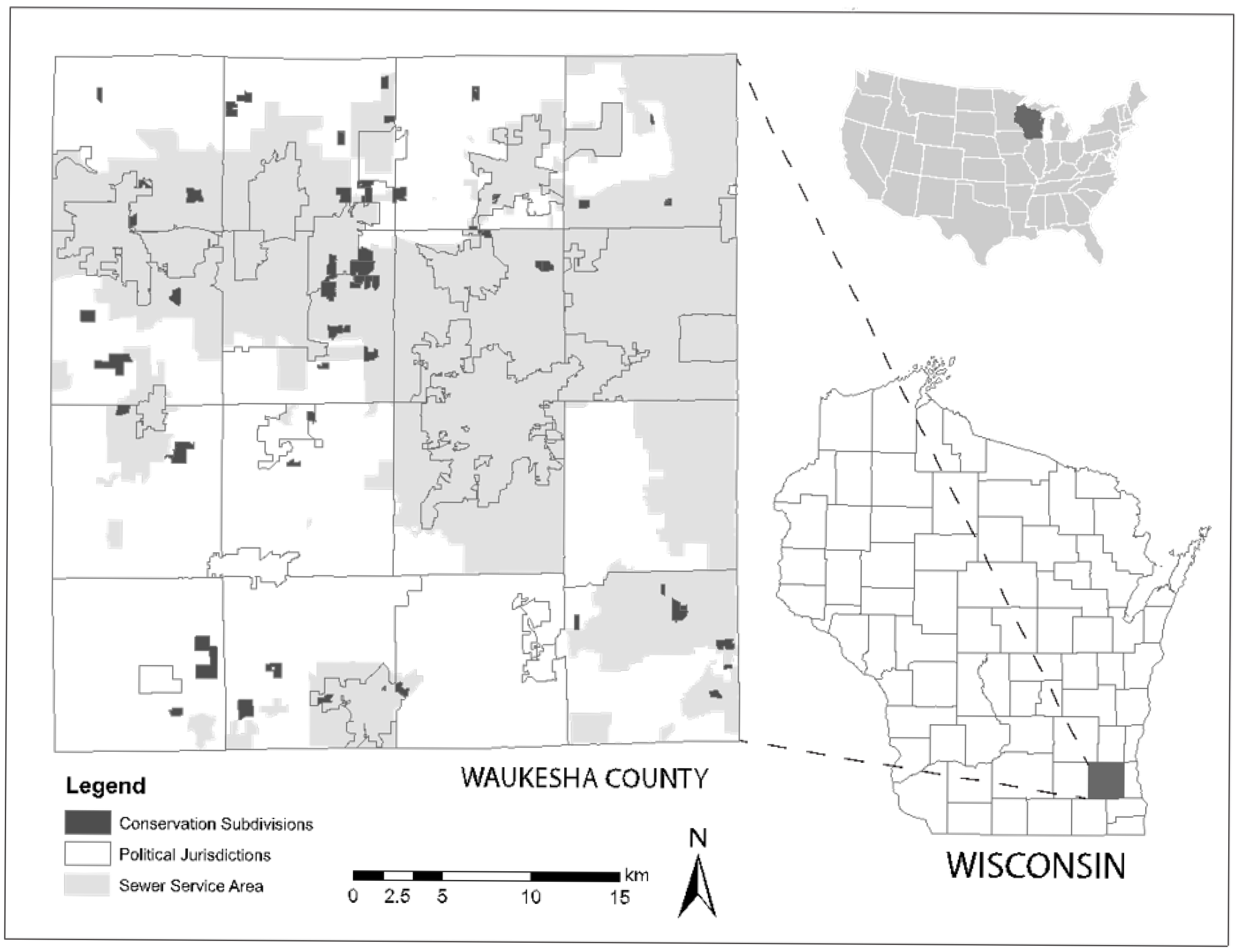
Our study focused on 54 conservation subdivisions in Waukesha County, in southeastern Wisconsin, USA. The State of Wisconsin has been estimated to rank third nationwide in the area of land developed as conservation subdivisions [14], and Waukesha County, primarily a suburban county, has the highest concentration of conservation subdivisions in the state. Waukesha County has experienced significant population growth resulting in high development pressures (especially between 1990 and 2000) and the loss of over 16,000 hectares of farmland between 1987 and 2007 [42,43,44]. According to the Southeastern Wisconsin Regional Planning Commission (SEWRPC), 54 conservation subdivisions were permitted in Waukesha County between 1990 and 2005. (Figure 1). SEWRPC [45] defines a conservation subdivision as “a housing development characterized by compact lots and permanent open space, where the natural features of the site are maintained to the greatest extent possible.”

2.2. Waukesha County Conservation Subdivisions

Our work is based on an analysis of the COS contained within the 54 Waukesha County conservation subdivisions, which we delineated and classified using GIS, aerial imagery, and field visits. In 2008, we received a list of conservation subdivisions built between 1990 and 2005 in the SEWRPC’s planning jurisdiction covering Waukesha County (G. Korb, personal communication 2008); we then confirmed with Waukesha County’s Department of Parks and Land Use staff that all of these subdivisions were those that planning agencies considered and promoted as conservation subdivisions.

In order to delineate subdivision COS, we obtained 2005 spatial data (the year marking the end of our investigation period) for subdivision boundaries, parcels, road right-of-ways, and environmental features from Waukesha County’s Department of Parks and Land Use, Land Information Systems Division. Once we located all COS for each subdivision, we used aerial photos to delineate the land cover and land use in COS; we updated these classifications in 2015 using 2015 imagery, and ground-truthed our classification via field visits, most recently in 2016. We classified each COS using eight broad categories of land cover and land use: woodland, naturally vegetated area (e.g., prairies, bushes, trees, but not woodlands), mown grass, open water, farmland, stormwater retention pond, gravel, and recreation (e.g., playground, basketball court).

2.3. Landscape Metrics Analysis

We calculated and compared landscape metrics of COS within and between these 54 conservation subdivisions using metrics quantifying the area, edge, isolation, and connectivity of patches to compare structure (composition and configuration) between landscapes. Landscape metrics were developed by landscape ecologists [46] as a means to quantify and compare structure among landscapes, or change within a landscape. Since then, many have tested and advanced the use of metrics in landscape studies [47,48,49,50]. In our study, we used FRAGSTATS (v. 4) to calculate seven class-level metrics to measure three broad characteristics: area/size, edge/shape, and aggregation/isolation (or fragmentation) (

Table 1. Landscape metrics used to assess composition and configuration of conservation subdivisions and their common open spaces.

Purpose/Category (Empirical Evidence)	Metric	Description or Definition	Value Interpretation
Area/Size	Proportion of the Landscape (PLAND)	Percentage of each class in the landscape (%)	The higher the value, the more area of that class exists.
(Freeman & Bell, 2011 [24]; Zhang et al. 2015 [31]; Corry & Nassauer 2005 [48]; Ackley et al. 2015 [51]; Ewers and Didham 2006 [52]; Shanahan et al., 2011 [53]; Vizzari and Sigura, 2015 [54]; Cunningham and Johnson, 2011 [55]; Cushman et al. 2008 [56]; Boongaling et al. 2018 [57]; Zhang et al. 2013 [58])	Mean Patch Size (MPS)	Average size of patches for each class (ha)	The higher the value, the less fragmented the class is.
	Large Patch Index (LPI)	Percentage of the landscape comprised by the largest patch (%)	Higher values indicate how much the class is dominated by a single large patch
Edge/Shape	Edge Density (ED)	Length of patch edge per unit area for each class	High values indicate greater edge to area ratio and potentially greater shape complexity
(Vizzari and Sigura 2015 [54]; Cunningham and Johnson 2011 [55])	Patch Density (PD)	Number of patches for each class per 100 hectare	High values indicate fragmented landscape
Aggregation/Isolation/Fragmentation	Landscape Shape Index (LSI)	Total length of patch edge within landscape divided by the total area adjusted by a constant	High values indicate that the class type is highly disaggregated.
(Corry & Nassauer 2005 [48]; Cushman et al. 2008 [56]; Van Nieuwenhuyse et al. 2011 [59])	Interspersion and Juxtaposition Index (IJI)	The observed interspersion over the maximum possible interspersion for the given number of patch types.	High values indicate that most patch types are equally adjacent to most other patch types.

Note: Please see FRAGSTATS documentation [64] for more information on the metrics.

) [51,52,53,54,55,56,57,58,59]. We calculated metrics for 1) the entire COS area (i.e., aggregated COS; COS_com), and within COS, we selected class-level landscape types of 2) woodland (COS_wood) and 3) natural vegetation (COS_nat). We conducted these separate analyses because woodland and natural vegetation provide benefits over other COS classes for biophysical processes such as provision of natural habitat for plant and wildlife species [60], critical plant-soil relationships [61,62], and infiltration of stormwater runoff [63]. We were not interested in several measures of composition such as richness or diversity since the other class types in our study area are less conducive to the provision of ecosystem services and natural habitat. Rather, we categorized the metrics used here by more specific aspects of landscape structure (area/size, edge/shape, aggregation/isolation) similar to the FRAGSTATS documentation.

We extracted all 54 conservation subdivisions from the GIS vector dataset such that each subdivision was analyzed as an individual landscape. We converted the vector datasets into raster datasets with a cell size of 0.304 m by 0.304 m (1 ft by 1 ft) for use in landscape metrics calculations. Patches were defined using the 8-cell neighbor rule.

We selected a suite of metrics relevant for assessing biophysical processes in urbanized and urbanizing areas [24,53,60,65,66,67], which allowed us to quantitatively distinguish landscapes from each other [55,56,68]. For the category of area/size, we measured proportion of the landscape (PLAND), mean patch size (MPS), and largest patch index (LPI); for edge/shape, we measured patch density (PD), and edge density (ED); we measured landscape shape index (LSI) and interspersion/juxtaposition index (IJI) to assess aggregation/isolation/fragmentation. We could only calculate IJI for unaggregated classes of woodland and natural vegetation because this metric is not valid when fewer than three classes exist in the landscape (i.e., the two classes consisting of COS and non-COS in the aggregated analysis). Because the 54 subdivisions all varied in total area, we respected the limitations in interpreting the values of metrics between these landscapes [64]. Based on our review of literature testing the sensitivity and behavior of landscape metrics to varying spatial extent [50,69,70], we chose metrics least sensitive to changing extent to represent each of the categories of landscape structure (for area/size: PLAND, LPI; for edge/shape: ED, PD; and for aggregation/isolation: LSI, IJI). These metrics were selected because previous empirical studies have demonstrated their value for characterizing ecologically relevant differences in habitat amount, patch size, edge exposure, shape complexity, and fragmentation/interspersion, while also indicating their suitability for comparisons across landscapes of differing extent. Finally, despite conflicting reports on the predictability of MPS [50,69,70], we included it in our analysis because patch size provides a critical and comparable metric for many ecosystem services. For detailed information on the metrics used in this study, see Table 1.

2.4. Statistical Analysis of Subdivision Common Open Space Landscape Structure

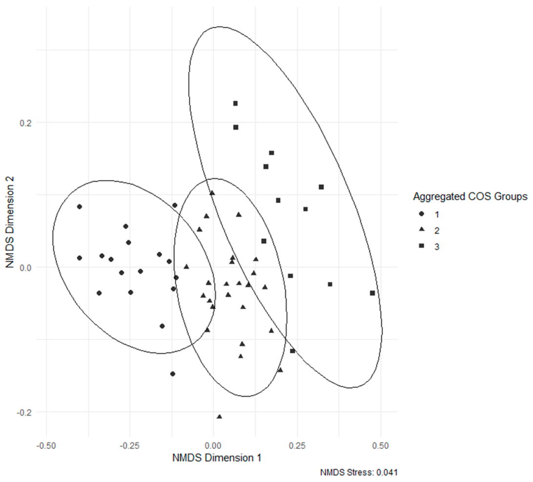
We used non-metric multidimensional scaling (NMDS), followed by k-means clustering of the ordination scores, to characterize and visualize differences in the landscape structure among conservation subdivisions. We selected NMDS based on Bray–Curtis dissimilarity over principal component analysis (PCA) as the primary ordination method because NMDS is robust to non-normal, skewed, and outlier-influenced data, common characteristics of FRAGSTATS class-level metrics. All NMDS solutions produced stress values ranging from 0.040 to 0.049. Because several input metrics were moderately to strongly correlated (e.g., PLAND–LPI, r = 0.79), and because Bray–Curtis dissimilarity, unlike PCA, does not correct for redundancy among correlated variables, results were cross-validated against an independent PCA ordination of the same standardized data. The two methods showed strong agreement for both axes in the COS_wood and COS_com datasets, with Procrustes disparities of 0.025 and 0.049, respectively. For COS_veg, the two methods showed strong agreement along Axis 1 but weaker correspondence along Axis 2, consistent with its higher Procrustes disparity of 0.248. A similar pattern was observed in the resulting cluster assignments, with adjusted Rand indices ranging from 0.419 to 1.000 across datasets. These results indicate that, although the degree of correspondence varied among the three classes, FRAGSTATS class-level metric redundancy did not substantially alter the overall NMDS-based classification (see Table S1).

Landscape metrics were standardized before the analysis so that all variables contributed equally to the ordination. K-means clustering was used to group the subdivisions with similar landscape characteristics by minimizing within-cluster variation while maximizing differences among clusters [71,72]. We evaluated cluster solutions ranging from 2 to 19 clusters and selected three clusters (k = 3) based on average silhouette width, bootstrap stability, and visual separation in the NMDS ordination (see Table S2). The first two NMDS axes were plotted to visualize differences in landscape structure, with subdivisions positioned closer together representing more similar landscape characteristics. All analyses were conducted in R using the vegan (v. 2.3–5) and fpc (v. 2.2–13) packages [73].

2.5. Analysis of Bird Occurrence in Waukesha County Conservation Subdivisions

In order to assess bird occurrence in Waukesha County conservation subdivisions, we used data that we obtained from eBird. A product of the Cornell Lab of Ornithology, eBird is an international citizen science project focused on the collection and cataloging of data specific to the distribution and relative abundance of bird species [74]. Downloadable for user-defined regions, this dataset provides information such as species, number of individuals seen, date of observation, GPS location, and the observer’s unique identifier. For the purposes of our analyses, we acquired data for Waukesha County for the years 2010 through 2020 and converted it to a format suitable for analyses in ArcGIS Pro (v. 2.8). One standout feature of eBird data is the flexibility it provides when conducting analyses, such as the ability to locate sightings by specific location using GPS coordinates.

In our analysis, we examined the total number of sightings (i.e., number of entries) and total number of observations (i.e., number of birds) in conservation subdivisions without distinguishing the type of species observed. This choice emphasizes overall bird use rather than species composition; species-specific analysis could be a valuable future extension. We assumed that the occurrence of birds is a potential proxy for ecosystem services supporting habitat provision. We used bird records as an exploratory indicator of bird use of conservation subdivisions rather than as a direct measure of habitat quality or ecosystem-service provision, as we did not measure characteristics such as species diversity, species survival rates, and presence of indicator species.

To assess the role of subdivision open space landscape structure on wildlife, we analyzed the differences in average eBird sightings and observations based on the landscape-metrics groupings of the subdivision total COS, woodland COS, and naturally vegetated COS. We also analyzed relationships between bird sightings and observations, and individual landscape metrics that we calculated.

3. Results

3.1. Landscape Metrics

The average area of conservation subdivisions in Waukesha County is 39 hectares, ranging from 6 hectares to 205 hectares with a gross density of 1.6 lots per hectare. Across these 54 conservation subdivisions, the proportion of the subdivision land set aside as COS (COS_com) ranged from approximately 14% to 80%. More specifically, total COS_com ranged from 0.9 to 93 ha, largest patch index from 6 to 78%, mean patch size from 0.8 to 27 ha, edge density from 9 to 210 m per ha, patch density from 1 to 37 patches per 100 ha, and landscape shape index from 1 to 9. The greatest variation in metrics across COS_com was found in mean patch size, followed by patch density, as indicated by the coefficient of variation (

Table 2. Landscape metrics for the aggregated, wooded, and naturally vegetated COS of Waukesha County conservation subdivisions.

n	54	49	50
	Aggregated COS	Woodland COS	Naturally Vegetated COS
Mean	18.7	7.2	7.7
SD	18.09	11.31	8.65
CV	96.73	157.23	112.37
Max	92.64	57.66	41.43
Min	0.9	0.17	0.07
Proportion of Landscape (%)
Mean	47.13	15.93	19.53
SD	13.43	13.14	13.4
CV	28.49	82.5	68.61
Max	80.08	54.28	63.99
Min	14.27	0.42	0.5
Mean Patch Size (hectares)
Mean	7.16	1.57	1.34
SD	6.15	3.18	1.57
CV	85.95	202.87	117.42
Max	27.23	18.27	8.17
Min	0.79	0.04	0.01
Largest Patch Index (%)
Mean	34.77	10.96	11.81
SD	16.79	11.51	11.44
CV	48.28	104.99	96.91
Max	78.13	47.93	59.72
Min	5.75	0.42	0.32
Edge Density (meters per hectare)
Mean	106.75	85.81	113.84
SD	46.03	48.86	63.14
CV	43.12	56.94	55.46
Max	210.33	199.81	257.64
Min	9.34	4.43	0
Patch Density (patches per 100 hectares)
Mean	11.13	24.27	23.32
SD	7.47	22.71	16.99
CV	67.11	93.56	72.85
Max	37.32	111.97	79.13
Min	1.46	2	4.01
Landscape Shape Index
Mean	3.63	4.29	4.91
SD	1.53	1.77	2.35
CV	42.07	41.33	47.85
Max	9.3	9.49	9.95
Min	1.03	1.44	1.35
Interspersion & Juxtaposition Index (%)
Mean	na	47.32	63.25
SD	na	19.65	23.05
CV	na	41.53	36.44
Max	na	82.14	93.71
Min	na	0	0

).

Across Waukesha County subdivisions, wooded COS could be as large as 58 hectares and naturally vegetated COS as much as 41 hectares in a subdivision. The proportion of wooded and naturally vegetated COS ranged from approximately 0% to 60% across both classes. In both vegetated types of COS, the greatest variation among the metrics was found in MPS, followed by LPI. In wooded COS specifically, variation in patch density across the conservation subdivisions was similar to that of LPI (Table 2). Apart from landscape shape index, variation in landscape metrics in both wooded COS and naturally vegetated COS analyses was greater when compared to metrics in the aggregated COS analysis. Naturally vegetated COS especially showed greater variability and potentially more sensitivity to configuration than aggregated COS.

3.2. Non-Metric Multidimensional Scaling

3.2.1. Overall COS Analysis

The k-means analysis for the subdivision (COS_com) partitioned the 54 conservation subdivisions into three groups of 17, 25, and 12 subdivisions (

Table 3. Groups of conservation subdivisions based on the k-means analysis of the landscape metrics of the aggregated COS.

	Groups
	1	2	3
n	17	25	12
Total Common Open Space Area (hectares)
Mean	29.08	17.60	27.46
SD	26.50	9.61	21.47
CV	91.10	54.58	78.18
Max	92.64	47.52	80.39
Min	4.86	5.96	7.22
Proportion of Landscape (%)
Mean	57.60	47.30	31.95
SD	11.86	8.31	9.61
CV	20.59	17.57	30.08
Max	80.08	62.98	44.81
Min	38.67	33.05	14.27
Mean Patch Size (hectares)
Mean	14.32	4.97	1.56
SD	5.91	1.78	0.55
CV	41.27	35.74	35.08
Max	27.23	9.50	2.37
Min	4.86	2.80	0.79
Largest Patch Index (%)
Mean	52.50	29.78	20.04
SD	12.63	10.75	9.73
CV	24.06	36.10	48.56
Max	78.13	55.64	34.72
Min	34.63	12.33	5.75
Edge Density (meters per hectare)
Mean	65.64	125.63	125.68
SD	36.71	33.09	45.24
CV	55.93	26.34	35.99
Max	136.08	210.33	207.08
Min	9.34	61.83	74.77
Patch Density (patches per 100 hectares)
Mean	4.67	10.36	21.88
SD	1.93	3.12	7.07
CV	41.35	30.16	32.31
Max	9.30	16.46	37.32
Min	1.46	5.23	9.07
Landscape Shape Index
Mean	2.69	4.14	3.89
SD	1.13	1.09	2.18
CV	41.92	26.21	56.10
Max	5.68	6.38	9.30
Min	1.03	2.68	1.68

, Figure 2). The three groups can be characterized as subdivisions with: (1) mostly intact COS with the largest mean patch sizes ($\underset{\_}{x}$= 14.3 ha ± 5.9 SD), smallest edge density ($\underset{\_}{x}$= 65.6 m/ha ± 36.7 SD), and the largest proportion of land set aside as COS ($\underset{\_}{x}$= 57.6% ± 11.8 SD); (2) fragmented COS with smaller patch sizes ($\underset{\_}{x}$= 5.0 ha ± 1.8 SD), a high degree of edge density ($\underset{\_}{x}$= 125.6 m/ha ± 33.1 SD) and a medium proportion of land set aside as COS ($\underset{\_}{x}$= 47.3% ± 8.3 SD); and (3) smallest ($\underset{\_}{x}$= 1.6 ha ± 0.6 SD) and dispersed patches with a high degree of edge density ($\underset{\_}{x}$= 125.7 m/ha ± 45.2 SD) and the least proportion of land set aside as COS ($\underset{\_}{x}$= 31.9% ± 9.6 SD) (Table 3; Figure 3). Subdivisions in Group 1, on average, had the largest patches with the smallest patch density. For example, in Walnut Grove (Figure 3a; MPS: 27 ha and PLAND 55%), residential lots are clustered around one large COS area in the center of the subdivision. Similar to Group 1, Group 2 contained subdivisions with a high proportion of COS, but in general the subdivisions in this group had a larger number of patches that were comparably smaller and more complex. For example, while the Hawks Nest subdivision (Figure 3b; MPS: 5 ha, PLAND: 46%) had a large proportion of COS, the COS was fragmented by the residential lots along the road network, which includes a centrally located loop and several extensions within and beyond the subdivision. Subdivisions in Group 3 had the lowest amount of land dedicated for COS when compared to Groups 1 and 2, and the COS patches in this group of subdivisions were, on average, the smallest with high fragmentation and dispersal. For instance, in Mary Hill (Figure 3c; MPS: 1 ha, PLAND: 32%), the residential lots are mostly located along narrow strips of COS patches, reflecting more of a “token” form of COS allocation compared to subdivisions in Group 1.

3.2.2. Woodland COS Analysis

The k-means analysis partitioned the woodland COS (COS_wood) landscape metric dataset into three groups of 5, 24, and 20 subdivisions. This analysis contained 49 conservation subdivisions because five conservation subdivisions did not contain wooded COS. The NMDS ordination (stress = 0.04) ranked the conservation subdivisions from those with large wooded patches to subdivisions with fragmented, smaller patches. When compared to the other two groups of subdivisions, the conservation subdivisions in Group 1 had the largest mean patch size ($\underset{\_}{x}$= 8.1 ha ± 6.9 SD) and proportion of landscape ($\underset{\_}{x}$= 43.4% ± 8.4 SD) but also had relatively large edge density ($\underset{\_}{x}$= 106.6 m/ha ± 52.8 SD) (

Table 4. Groups of conservation subdivisions based on the k-means analysis of the landscape metrics of the wooded COS.

	Groups
	1	2	3
n	5	24	20
Woodland Cover Class Common Open Space Area (hectares)
Mean	27.51	6.08	3.46
SD	21.52	5.28	8.20
CV	78.22	86.86	19.45
Max	57.66	19.17	37.74
Min	7.39	0.39	0.17
Proportion of Landscape (%)
Mean	43.38	19.07	5.29
SD	8.44	7.65	4.54
CV	19.45	40.10	19.45
Max	54.28	32.40	18.37
Min	32.77	4.85	0.42
Mean Patch Size (hectares)
Mean	8.12	0.86	0.77
SD	6.85	0.80	1.49
CV	84.33	92.61	84.33
Max	18.27	3.56	6.43
Min	2.46	0.04	0.09
Largest Patch Index (%)
Mean	37.05	12.03	3.15
SD	9.07	7.16	3.23
CV	24.49	59.49	24.49
Max	47.93	28.77	12.88
Min	24.98	0.91	0.42
Edge Density (meters per hectare)
Mean	106.58	120.44	39.07
SD	52.78	27.77	24.16
CV	49.53	23.06	49.53
Max	174.17	199.81	87.64
Min	37.44	73.56	4.43
Patch Density (patches per 100 hectares)
Mean	9.53	36.81	12.90
SD	7.11	25.93	9.27
CV	74.60	70.44	74.60
Max	19.82	111.97	37.18
Min	2.11	5.96	2.00
Landscape Shape Index
Mean	4.16	4.84	3.65
SD	2.57	1.67	1.53
CV	61.85	34.54	61.85
Max	7.83	9.49	7.01
Min	1.77	1.79	1.44
Interspersion & Juxtaposition Index (%)
Mean	41.74	52.22	42.85
SD	32.20	16.43	19.26
CV	77.14	31.47	77.14
Max	73.30	82.14	64.18
Min	5.43	19.79	0.00

). Eagles Preserve subdivision (Figure 4a), for instance, had a large COS (56%) surrounding most of its residential lots, with the majority of its COS being a few large wooded patches (MPS: 12 ha, PLAND: 42%). The subdivisions in Group 2 had a medium amount of COS in woodland, which was in small ($\underset{\_}{x}$= 0.9 ha ± 0.8 SD), fragmented, and dispersed patches and proportion of landscape ($\underset{\_}{x}$= 19.1% ± 7.7 SD) with high edge density ($\underset{\_}{x}$= 120.4 m/ha ± 27.8 SD). For example, the Lakewood Farms Preserve subdivision (Figure 4b) had its wooded COS fragmented into several patches dispersed throughout the subdivision due to the layout of the residential lots and the presence of other COS land covers and uses (MPS: 2 ha, PLAND: 24%). The conservation subdivisions in Group 3 had the smallest proportion of wooded COS ($\underset{\_}{x}$= 5.3% ± 4.5 SD), which was commonly in small patches ($\underset{\_}{x}$= 0.8 ha ± 1.5 SD) with the lowest edge density of the 3 groups ($\underset{\_}{x}$= 39.1 m/ha ± 24.2 SD). For example, the Mary Hill Park subdivision (Figure 4c) has a few small wooded COS patches on the south side of the subdivision (MPS: 0.2 ha, PLAND: 4%).

3.2.3. Naturally Vegetated COS Analysis

According to the k-means analysis of the naturally vegetated (non-forested) COS (COS_nat), the 50 Waukesha County subdivisions all with naturally vegetated COS were partitioned into three groups: 9, 18, and 23 subdivisions (Figure 5). The NMDS ordination (stress = 0.05) arranged the conservation subdivisions ranging from large-patch subdivisions to fragmented and smaller-patch subdivisions (Figure 5). Subdivisions in Group 1 typically had higher proportions of land in natural vegetated COS ($\underset{\_}{x}$= 40.5% ± 10.5 SD), with larger patches ($\underset{\_}{x}$= 3.7 ha ± 2.2 SD) (See

Table 5. Groups of conservation subdivisions based on the k-means analysis of the landscape metrics of the naturally vegetated COS.

	Groups
	1	2	3
n	9	18	23
Naturally Vegetated Cover Class Common Open Space Area (hectares)
Mean	10.58	9.43	5.20
SD	4.37	10.35	8.03
CV	41.27	109.68	154.29
Max	17.80	41.43	39.05
Min	3.39	0.07	0.20
Proportion of Landscape (%)
Mean	40.45	17.65	12.82
SD	10.47	7.96	9.05
CV	25.89	45.11	70.64
Max	63.99	32.21	28.99
Min	30.78	1.05	0.50
Mean Patch Size (hectares)
Mean	3.73	0.65	0.95
SD	2.22	0.58	0.75
CV	59.60	90.07	79.06
Max	8.17	2.59	3.00
Min	1.13	0.01	0.07
Largest Patch Index (%)
Mean	30.49	8.03	7.46
SD	13.73	4.52	5.75
CV	45.03	56.28	77.12
Max	59.72	16.17	17.63
Min	13.73	0.67	0.32
Edge Density (meters per hectare)
Mean	142.59	161.92	64.97
SD	48.65	49.08	37.82
CV	34.12	30.31	58.21
Max	232.94	257.64	131.00
Min	61.97	51.03	0.00
Patch Density (patches per 100 hectares)
Mean	14.00	38.57	15.03
SD	7.06	18.34	8.19
CV	50.39	47.54	54.53
Max	27.89	79.13	33.44
Min	5.24	12.44	4.01
Landscape Shape Index
Mean	3.97	7.01	3.63
SD	0.95	2.09	1.71
CV	24.00	29.77	46.99
Max	5.08	9.95	8.06
Min	2.75	3.99	1.35
Interspersion & Juxtaposition Index (%)
Mean	76.38	67.22	55.00
SD	9.08	20.84	25.75
CV	11.88	31.00	46.82
Max	93.71	89.01	91.26
Min	64.13	0.00	0.00

), but also with relatively high edge density ($\underset{\_}{x}$= 142.6 m/ha ± 48.7 SD). For example, Mason Creek had a relatively large COS (65%), primarily made up of natural vegetation, that was divided by the road network and residential lots (Figure 5a; MPS: 3 ha, PLAND: 38%). The subdivisions in Group 2 had, on average, a lower proportion of land in COS that was naturally vegetated ($\underset{\_}{x}$= 17.7% ± 8.0 SD), which were found in small patches ($\underset{\_}{x}$= 0.7 ha ± 0.6 SD) with a high edge density ($\underset{\_}{x}$= 161.9 m/ha ± 49.1 SD) when compared to Group 1 subdivisions on average. For example, the Preserve at Hunter Lake subdivision (Figure 5b; MPS: 0.4 ha, PLAND: 12%) had a large portion of its land dedicated to COS, with many small naturally vegetated COS patches dispersed across the subdivision. Finally, the conservation subdivisions of Group 3, which had the greatest variability on the COS_nat metrics (see Table 4), had the smallest proportion of COS ($\underset{\_}{x}$= 12.82% ± 9.1 SD) with few small patches ($\underset{\_}{x}$= 1.0 ha ± 0.8 SD) and the lowest edge density ($\underset{\_}{x}$= 65.0 m/ha ± 37.8 SD) of the three groups. The large variability in the metrics, as indicated in the table and in the NMDS ordination, suggests that these subdivisions did not form a category that can be easily (or distinctly) categorized. Because there was great variability, we did not choose a subdivision to display and examine.

3.3. Wildlife Occurrence in Conservation Subdivisions

According to eBird data between 2010–2020, 461 sightings have been recorded within 17 of the 54 Waukesha County conservation subdivisions we studied, which amounted to 1301 observations. There was no record of birds in 37 of the 54 subdivisions during this period; we did not include those subdivisions in our analysis. Sightings ranged from 1 to 284, the number of birds observed ranged from 1 to 902, and the number of species of birds observed ranged from 1 to 39 in the 17 subdivisions.

3.4. Wildlife–Conservation Subdivision COS Landscape Structure Connection

We analyzed the differences in means of bird sightings and observations based on the landscape structure groupings of conservation subdivisions for aggregated COS, wooded COS, and naturally vegetated COS (

Table 6. Analysis of bird sightings and observations and COS landscape structure.

COS Type		Group 1	Group 2	Group 3
	n	6	7	4
COS_com	Sightings	52.17 (113.68)	17.71 (22.61)	6 (10.00)
	Observations	160.17 (363.55)	39.14 (59.10)	16.5 (31.00)
	n	2	7	7
COS_wood	Sightings	7.5 (9.19)	14.71 (18.38)	48.86 (104.05)
	Observations	14 (23.33)	34.29 (60.66)	147.43 (333.48)
	n	2	5	8
COS_nat	Sightings	153 (185.26)	8.2 (5.26)	13.5 (11.62)
	Observations	470 (610.94)	15.4 (10.06)	34.13 (432.00)

). Our analysis found that subdivisions in Group 1 for aggregated COS, which had the largest mean patch sizes, smallest edge density, and the largest proportion of land set aside for COS, indeed had the highest number of bird sightings and observations. Similarly, subdivisions in Group 3 that had the lowest amount of COS dedication and smallest patch sizes on average, with fragmented and dispersed patches, had the lowest number of bird sightings and observations. Yet, the differences in the means were not significant. We did not find any significant correlations between bird sightings and observations and individual landscape metrics. The only noteworthy difference was in the amount of aggregated COS; the subdivisions in the top quartile for amount of aggregated COS had significantly higher numbers of bird sightings and observations compared to the subdivisions in the lowest quartile based on the total area of COS.

Our analysis of wooded COS similarly did not yield statistically significant differences among bird sightings or observations (Table 6). Neither did we find significant correlations between bird sightings/observations and individual landscape metrics in general for wooded COS. However, we found statistically significant differences between the subdivisions in Groups 1 and 3 based on the naturally vegetated COS classification. Subdivisions in Group 1 had significantly more sightings and observations compared to subdivisions in Group 3. We also found significant correlations between sightings/observations and metrics associated with the naturally vegetated COS. More specifically, the proportion of COS that was naturally vegetated and the largest patch index for naturally vegetated COS were strongly, significantly, and positively associated with bird sightings and observations. Moreover, mean patch size was strongly, significantly, and positively associated with bird sightings and strongly and positively associated with observations.

4. Discussion

The analysis of the 54 conservation subdivisions in Waukesha County, Wisconsin revealed that the landscape structure of COS varied considerably across the conservation subdivisions. On average, while nearly half of the subdivision land was set aside in COS, that proportion ranged from 14% to 80%. Among the landscape metrics we examined, mean patch size and patch density varied the greatest (the coefficient of variation for these metrics was greater than 67%).

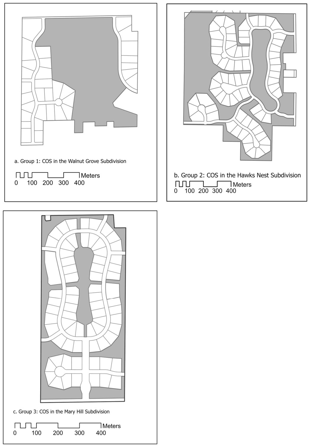
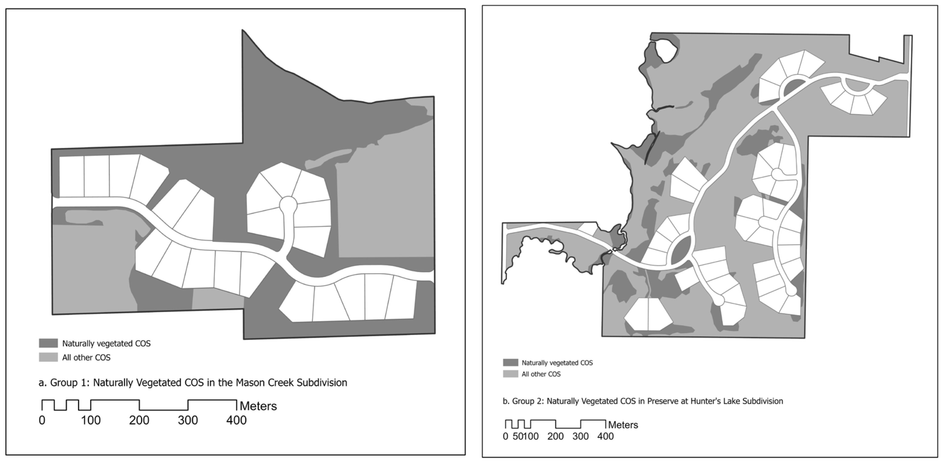
Our study provided evidence of distinct patterns in the landscape structure of the COS despite the large overall variability. Specifically, conservation subdivisions separated into three discernible groups, relative to one another: (1) subdivisions with large, non-fragmented or minimally fragmented open space with a relatively small amount of edge, (2) subdivisions with medium size but fragmented common open space with a high degree of edge (double in comparison to Group 1), and (3) subdivisions with small, fragmented open space with similar edge density as Group 2.

The majority of subdivisions in Group 1 consisted of residential lots clustered around one large COS area, with few to no roads or residential lots fragmenting the COS. According to the three metrics we used to evaluate area and size (PLAND, MPS, and LPI), COS in this group on average was the largest among the three subdivision groups; for instance, the mean value for MPS in this group was 14.32 hectares as opposed to the mean value of 4.97 hectares (Group 2) and 1.56 hectares (Group 3). The COS in subdivisions in Group 1 also had the least amount of edge on average relative to subdivisions in the other two groups, as well as the least amount of fragmentation or isolation. Patch size in urbanized landscapes can be critical for ecological processes. In this matter, our analysis of eBird sightings and observations showed that this group of subdivisions had a higher number of sightings and observations, but without differences compared to the other groups of subdivisions. Area of open spaces appeared to play another important role within Waukesha County conservation subdivisions as well; subdivisions in the top quartile based on area of COS had more eBird observations recorded compared to the subdivisions in the bottom quartile, implying that the larger open spaces may support birds to a greater extent. It is critical to note that landscape structure represents a potential driver of ecosystem services rather than direct evidence of ecosystem functioning. Similarly, bird observations are considered as an exploratory indicator of bird use of conservation subdivisions rather than as a direct measure of habitat quality or ecosystem-service provision.

We recognize the limitations of using citizen data in lieu of systematic observations based on proven methods that involve sampling and thorough surveys. Most importantly, the absence of bird observations in a subdivision does not necessarily mean that birds were not present, as we did not conduct an occupancy analysis and evaluate detectability. Moreover, variation in bird observations among conservation subdivisions may reflect accessibility and popularity of the eBird tools as well as observer interest, knowledge, and effort. These types of data may erroneously identify clusters of birds in an area because of interested and knowledgeable observers residing in some subdivisions and not in others. We want to caution our readers about another aspect of using eBird data in our work. The delineation and verification of the COS (the latest being 2016) and the eBird data (2010–2020) timelines do not match precisely. We did not have the capacity to undertake verification efforts after 2016, while desiring to get more recent bird data to reflect more complete construction and land management in conservation subdivisions that were permitted and had at least begun construction by 2005 (the end date of our conservation subdivisions dataset). We recognize that landscape structure may have changed between 2016 and 2020.

In future studies looking at ecosystem services in the conservation subdivisions we examined, we hypothesize that the larger patches of Group 1 will provide greater ecosystem services when compared to several smaller, isolated patches (see, for instance, [30]). For example, a larger patch may result in a greater level of water infiltration, as large patch and aggregation indices were found to positively correlate with runoff reduction [31]. Moreover, habitat provision for human-sensitive, non-synanthropic species may be greater in subdivisions with larger, more intact patches because they reduce edge effects and human disturbance, increase interior habitats, may support larger populations and colonization rates, and may decrease predator invasions [23,53,75,76]. Related to patch size and shape is edge density, which may dictate what types of wildlife are able to occupy the patch. For example, increasing the amount of edge habitat can increase densities of edge-loving species like white-tailed deer (Odocoileus virginianus) and other common wildlife, potentially increasing human-wildlife conflicts [29]. However, we cannot assume that reduced fragmentation would benefit biodiversity in every context. Habitat loss generally has strong negative effects on biodiversity, but the independent effect of fragmentation—that is, the spatial subdivision of a fixed amount of habitat—can be negative, neutral, or positive [77,78,79]. Smaller or more dispersed patches may increase habitat heterogeneity, landscape complementation, or access to resources for some edge-associated and disturbance-tolerant species. Accordingly, larger patches, lower edge density, and lower fragmentation are most likely to benefit species whose habitat use, movement, reproductive success, or persistence is adversely affected by edges, disturbance, or limited interior habitat. The biodiversity implications of conservation subdivision design therefore depend on the ecological requirements of the species present, the amount and quality of retained habitat, and the composition of both the common open space and the surrounding residential matrix.

Given the importance of habitat area, we would still expect Group 1 to support larger numbers of birds and other wildlife, and more specifically we would predict interior bird species to increase with increasing patch size. In Groups 2 and 3, we would predict an increasing number of edge-associated bird species with increasing amounts of fragmentation and edge.

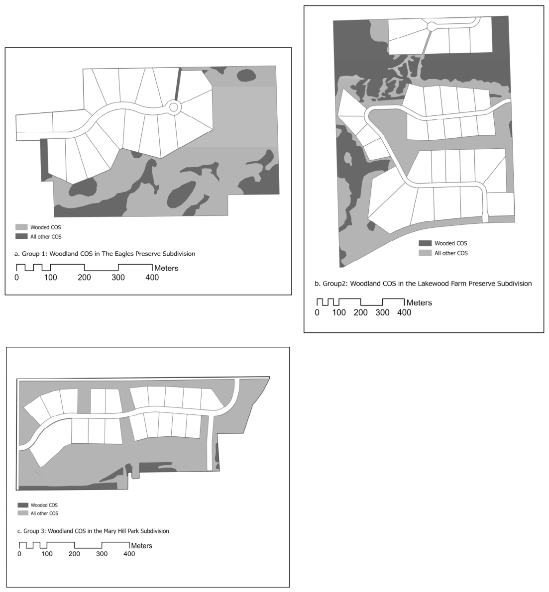
Similar to total COS landscape structure, we found variability of COS composition and configuration when we examined woodland and natural vegetation land cover classes separately. Many studies have found landscape composition, particularly the proportion of a particular land cover type, to be important for ecosystem services [80,81,82]. Both land cover types of woodland and natural vegetation in Group 1, on average, exceeded 40% in our analysis. These averages were lower in subdivisions in Groups 2 (19% wooded and 18% naturally vegetated) and 3 (5% wooded and 13% naturally vegetated). Indeed, a few of the subdivisions in Groups 2 and 3 contained COS largely maintained as mown lawn. Compared to turf, wooded or naturally vegetated land cover can provide greater regulation of air and soil quality, infiltration of stormwater runoff, evaporative cooling, reduced soil compaction, and pollutant removal [31,57,58,61,62]. Relative to the diversity of birds and use by mammals, Farr et al. [23] found that the presence of natural land covers within and surrounding COS was important. Likewise, in a study of bee abundance in relation to urban development, Pfeiffer et al. [83] noted an effect of local land cover, such as impervious surface, on soil-nesting bees, and these effects were greater in newer neighborhoods. Additionally, species-dependent, large forested patches are more likely to maintain avian species richness and integrity than small forested patches [84,85], but see [77]. Similarly, there is evidence that large forested patches reduce sediment yield and stormwater runoff while increasing soil drainage and groundwater recharge [57,58]. In addition, large vegetated patches with low amounts of edge typically contain more native species [86]. Differing from these studies, our findings using eBird data did not find differences or associations with respect to wooded open space patches; however, this could simply be because of the limitations of eBird data. For instance, it may be harder for subdivision residents to observe birds in wooded areas compared to more open naturally vegetated areas such as prairies and mown COS found in many of these Wisconsin conservation subdivisions, and even compared to backyards. The associations found with bird sightings and observations and several of the landscape metrics in the groups of subdivisions based on naturally vegetated COS indicate the potential importance of conservation efforts and landscape structure of open spaces in residential areas. Despite the limitations of citizen science data, Callaghan et al. [87] stressed that eBird data may be a potentially reliable source in urban green spaces, and as such, in assessing suburban and exurban residential subdivision open spaces, it may similarly be an important source when other data are not available. We emphasize that our assessment of conservation subdivisions with eBird data is the first step toward understanding wildlife use of COS and not a definitive estimate of biodiversity or habitat quality.

Even though our study did not evaluate why there may have been significant variations in the landscape structure of COS in Waukesha County conservation subdivisions, prior empirical work on the implementation of these subdivisions shed light on some of these potential factors [88,89]. For instance, Göçmen identified a wide range of open space requirements among Waukesha County’s municipal zoning ordinances, with several municipalities not identifying a minimum areal percentage dedication to COS, what kinds of land should be in COS, or the extent to which ecologically significant lands should be protected in COS [88]. Municipal land permitting process also appeared to impact the landscape structure of the subdivisions. For instance, on multiple occasions, developers were asked to provide a “green” buffer around the residential areas to offset the perception of higher density in conservation subdivisions due to smaller lots, potentially leading to designs as observed in Mary Hill subdivisions in Figure 3b [88]. Examining developers’ perspectives also revealed significant differences in how they approached conservation subdivisions and COS; for instance, some developers based COS determination on the local land use regulations or economics of what might sell more easily or for more, while others delineated COS for its ecological benefit, including the region’s environmental corridors [89]. We suggest a future research direction that involves the factors that play a role in the COS compositions and configurations we have found in the three different groupings.

It is important to note that although there is no unifying or universal definition of what constitutes conservation subdivision, it would appear from our analysis that only subdivisions in Group 1, on average, would potentially qualify for what constitutes a conservation subdivision. No groups of subdivisions, on average, met SEWRPC’s guidelines of 60% land set aside in unsewered locations or Arendt’s [17] recommendation of setting aside a minimum of 50% of buildable lands. Only 10 out of the 54 (19%) conservation subdivisions had greater than Arendt’s suggested 50% of buildable lands set aside for subdivision COS. Future work could examine ecosystem services in subdivisions meeting regional or Arendt’s guidelines and evaluate whether those subdivisions meeting guidelines perform significantly better than those falling short of guidelines. In the case of no significant differences, future work could also seek to identify thresholds in COS amount and landscape metrics that provide substantial benefits.

5. Conclusions

Empirical work has suggested that local policy, regulations, and review processes do not always include evidence-based guidelines or make it easy to design conservation subdivisions to provide ecological benefits [8,88,90]. However, important guidelines have been provided for improving the design of conservation subdivisions to achieve ecological benefits. For instance, Carter [41] suggested that conservation subdivisions need to include specific language about the ecological integrity and long-term protection of the COS. Pejchar et al. [40] suggested that a scientific assessment of the ecological importance of a development site needs to be conducted to understand the parts of the property that need to be protected and restored and how the other parts of the property can be developed without jeopardizing the ecology of the site. Based on such an assessment, targeted ecosystem services or species habitat may be identified. With that information, concrete planning guidelines could be written specific to the development site and targets, defining criteria such as minimum patch size, maximum edge density, or target proportions of natural vegetation. Without specific targets identified, however, it is not possible to set landscape structure-based planning recommendations.

It is important to note that there remains a lack of explicitly documented relationships between landscape indices and ecological function, and studies have cautioned against making ecological inferences from landscape indices [48,49,91]. Although Corry and Nassauer [48] identified several limitations to making ecological inferences from landscape indices, especially in fine-scale patterns of highly fragmented habitats, they acknowledge the utility of indices as a first approximation of landscape patterns, and in characterizing differences among planned or design alternatives (see also [92]). It is also important to note that different metrics can have different associations with particular ecological functions and ecosystem services. Furthermore, this analysis considered landscape structure in a static sense, without attention to landscape connectivity—the ability of species and ecosystem services to move dynamically across space. As Bolliger and Silbernagel [93] argue, further work on connectivity assessments will be needed to better ground planning and design decisions for multi-functional landscapes such as green infrastructure and conservation subdivisions.

The kind of analysis presented in our manuscript has strong potential to be replicated, to contribute to the literature on conservation subdivisions, and to lay the foundation for future work to predict, test, and understand the impact of COS composition and configuration. Examples of future work on predicting, testing, and understanding the impact of COS composition and configuration include regulating classes of ecosystem services such as stormwater management through modeling stormwater runoff and supporting classes of ecosystem services such as habitat provisioning through systematic bird, mammal, and other species surveys.

To the best of our knowledge, this is the first empirical study to quantitatively assess the patterns of COS composition and configuration in conservation subdivisions. Our study identified that the implementation of conservation subdivisions varied widely, and that was only on a local level. If this variability is reflected on a regional or national scale, it is important that future research begin connecting how COS variability within conservation subdivisions impacts ecosystem services.