Seasonal and Multiscale Associations Between Surface-Water Fraction and Daytime Land Surface Temperature in the Wuhan Urban Agglomeration, China

Abstract

Surface water is an important component of urban land-cover systems, but its relationship with land surface temperature (LST) is difficult to interpret in lake-rich urban agglomerations where water bodies, shorelines, vegetation, built-up land, and terrain are closely interwoven. This study examined the association between surface-water fraction and daytime LST in the Wuhan Urban Agglomeration, China, across six benchmark years from 2000 to 2025. MODIS daytime LST, Landsat-derived water maps, GHSL built-up data, vegetation indices, and terrain variables were integrated on a 250 m grid. Surface-water fraction was measured within each grid cell and surrounding windows from 250 to 2000 m. Summer and winter models were compared, and between-location differences were separated from within-location water-fraction changes. Spatial validation, city-specific models, and robustness checks were used to assess consistency. Higher surface-water fraction was associated with lower daytime LST in both seasons. The strongest standardized association occurred at 500 m in summer, whereas the winter association strengthened toward 2000 m. Between-location differences were much larger than within-location changes, and the negative association was retained across all cities. These results suggest that surface-water fraction should be interpreted as a scale- and season-dependent land-cover indicator rather than as a fixed cooling measure.

1. Introduction

Urban land-cover change has become an important driver of surface thermal differentiation in rapidly urbanizing regions. As cities expand, vegetated, wet, and permeable surfaces are increasingly replaced by impervious land, altering surface energy exchange and increasing spatial variation in land surface temperature (LST). Blue–green landscape elements, including rivers, lakes, wetlands, riparian vegetation, and connected open spaces, are therefore important for understanding urban surface thermal patterns. Surface water is a key component of this landscape context because it connects open water, shoreline vegetation, riparian spaces, and adjacent built-up land [1,2,3].

Water surfaces respond differently to daytime heating than built-up and other non-water surfaces. Evaporation can consume part of the available energy, while the relatively high heat capacity of water may slow surface warming. Areas with more surface water therefore often exhibit lower daytime land surface temperatures than nearby impervious or dry surfaces [4,5,6,7]. Although land surface temperature (LST) does not directly represent near-surface air temperature or human heat exposure [8,9], it provides spatially continuous information on surface thermal patterns and is widely used to examine urban land–temperature relationships [10].

However, the relationship between surface water and LST varies across water bodies and urban settings. Water body size, shape, depth, shoreline characteristics, and hydrological conditions can affect the temperature contrast between water and surrounding land [7,9,11]. The surrounding environment is also important, particularly vegetation cover, impervious surfaces, urban density, and terrain [12,13]. Recent LULC–LST studies have further shown that water bodies, vegetation, built-up land, topography, and other underlying surfaces can contribute differently to surface thermal patterns across places and observation periods [14,15]. As a result, the observed water–LST relationship may reflect both water coverage and the environmental conditions around the water body [16,17]. It is better understood as a context-dependent association than as a response to water coverage alone.

The relationship between surface water and LST also varies by season [4,11,18]. In summer, strong solar radiation and high evaporative demand can increase the temperature difference between water and surrounding impervious surfaces. In winter, weaker radiation and lower evaporation may reduce this difference, while water may cool more slowly than adjacent land because of its greater thermal inertia. Previous studies have generally reported stronger cooling-related associations during warm periods. Winter patterns are more variable, with differences in magnitude and, in some cases, direction across study areas. Such variability may be related to regional climate, water-body characteristics, observation time, and the surrounding urban environment. Moreover, most existing studies have examined a single city, an individual lake or river, or a small number of observation dates. Whether the seasonal water–LST relationship remains consistent across cities and spatial contexts within a large urban agglomeration therefore remains unclear [16,19].

Seasonal differences in the water–LST relationship may also depend on the spatial scale at which surface water is measured [11,17,20,21,22,23]. Water fraction within a single grid cell mainly represents the immediate land–water composition around the temperature observation, whereas measurements over larger areas summarize water coverage within a broader landscape. The estimated relationship may therefore change with spatial scale. However, previous studies have often relied on a single buffer distance or a limited number of predefined zones, making it difficult to determine whether the observed relationship depends on the selected scale. Comparing multiple measurement supports can therefore help determine whether the observed association is more closely linked to immediate water coverage or to the broader surrounding landscape.

Regional water–LST relationships may also combine differences among locations with changes occurring at the same location over time. Lake-rich areas often have lower LST than densely built inland areas, but they may also differ in vegetation, urban form, and terrain. The resulting spatial contrast therefore cannot be interpreted directly as the temperature response to a change in water fraction at a fixed location [24,25]. Separating these two components provides a clearer basis for interpreting regional patterns. It also helps assess whether the identified relationship remains consistent across cities with different water systems, built-up conditions, terrain, and thermal backgrounds [26,27]. In lake- and river-connected urban regions, this issue is particularly important because water bodies are often embedded within wetlands, riparian vegetation, agricultural lowlands, and expanding built-up areas. Recent studies of riverine cities have shown that land-use dynamics, water bodies, vegetation, precipitation variability, and urban expansion can jointly shape thermal environments [28]. Although previous studies have shown that water–LST relationships can vary with season, scale, and surrounding landscape, fewer studies have examined how surface-water fraction should be interpreted across multiple measurement supports, within–between components, and cities within a lake- and river-connected urban agglomeration [6,16,19].

The Wuhan Urban Agglomeration is well suited to examining these questions because it includes a large metropolitan core, several smaller cities, extensive lakes and river networks, agricultural plains, hilly areas, and rapidly expanding built-up land. These contrasting environments create marked differences in hydrological conditions, urban development, and surface temperature patterns across the region. Using data from six representative years between 2000 and 2025, this study examined the relationship between daytime LST and surface water fraction while accounting for vegetation, built-up intensity, and terrain. Water fraction was calculated at the grid-cell level and within square windows with side lengths ranging from 250 to 2000 m.

This study examined the seasonal and scale-dependent relationship between surface-water fraction and daytime LST in the Wuhan Urban Agglomeration. Three questions were addressed. First, how does the water–LST association change between summer and winter, and does its scale-response pattern remain consistent across seasons? Second, how much of the water–LST relationship is explained by between-location differences, and how much by within-location water-fraction changes? Third, can the relationship remain consistent when tested in spatially independent areas and across different cities within the agglomeration?

Compared with studies focused on a single water body, a single city, or a fixed buffer distance, this study examines the surface-water fraction–LST relationship within a broader urban agglomeration and land cover context. Surface-water fraction was measured from the 250 m analytical cell to 2000 m surrounding windows, allowing the same relationship to be compared across multiple spatial supports. The analysis further separated persistent between-location differences from within-location water-fraction changes and evaluated spatial consistency through blocked validation, city-specific models, and leave-one-city-out testing. This design helps clarify whether surface-water fraction mainly reflects immediate land–water composition, wider river–lake and blue–green landscape context, or temporal changes at fixed locations.

2. Materials and Methods

2.1. Study Area and Temporal Design

This study focused on the Wuhan Urban Agglomeration in Hubei Province, China, which includes nine municipal units: Wuhan, Huangshi, Ezhou, Xiaogan, Huanggang, Xianning, Xiantao, Qianjiang, and Tianmen. Municipal administrative boundaries were obtained from the National Geomatics Center of China (NGCC) and used to delineate the study area, support municipal stratification, and conduct city-level heterogeneity and cross-city transfer analyses. The region contains a large metropolitan core, smaller surrounding cities, major river corridors, dense lake systems, agricultural plains, and hilly margins. These hydrological, urban, and terrain contrasts provide a suitable setting for examining seasonal associations between surface-water fraction and daytime land surface temperature (LST).

Summer and winter were analyzed separately because seasonal differences in radiation, vegetation cover, and moisture availability can alter the thermal contrast between surface water and surrounding land. In the Wuhan Urban Agglomeration, summer is generally warm and humid with stronger daytime heating, whereas winter is cooler, with weaker radiation and different vegetation and moisture conditions. Six representative benchmark years were selected at five-year intervals: 2000, 2005, 2010, 2015, 2020, and 2025. Summer observations covered the period from 1 June to 31 August in each target year. Winter observations covered the period from 1 December of the previous year to 28 or 29 February of the target year; for example, winter 2025 used observations from 1 December 2024 to 28 February 2025.

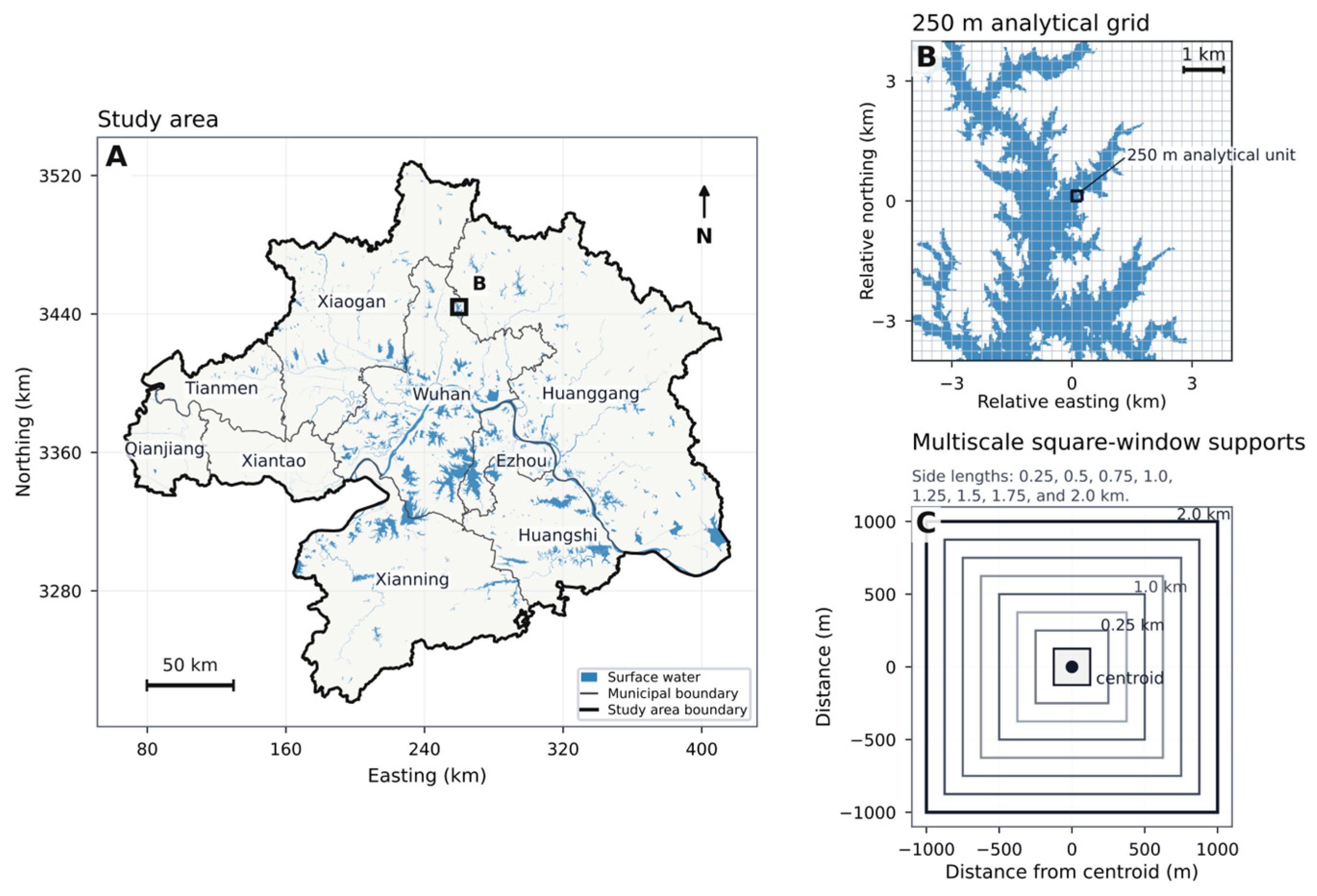
All spatial processing was conducted in WGS 84/UTM zone 50N (EPSG:32650), allowing grid construction, square-window extraction, and area calculations to be performed in meters. The analytical unit was a 250 m × 250 m grid cell. From the complete balanced panel, 60,000 grid cells with valid records in all twelve year–season periods were selected, yielding 720,000 observations. To ensure coverage of different cities and land-cover settings, the sample was selected using proportional stratification by municipality, surface-water fraction class, and built-up fraction class. Surface-water and built-up fractions were each grouped into four classes: zero (=0), low (>0–0.05), medium (>0.05–0.30), and high (>0.30–1.00). The same set of sampled grid cells was retained across all periods and subsequent analyses to maintain comparability among model results. The study area, analytical grid, and multiscale measurement design are illustrated in Figure 1.

2.2. Remote-Sensing Data and Product Preparation

Table 1. Data products, auxiliary layers, and analytical roles.

Dataset/Product	Main Variable	Resolution/Spatial Support	Temporal Coverage	Analytical Role
MODIS MOD11A2 V061	Daytime LST	Approximately 1 km; 8-day composite	Twelve seasonal periods for the six benchmark years	Parent thermal product; native-MODIS sensitivity analysis
RF-A downscaled LST	250 m daytime LST	250 m analytical grid	Same twelve seasonal periods	Primary thermal response variable
RF-B sensitivity LST	Water-sensitive downscaled LST	250 m analytical grid	Same twelve seasonal periods	Downscaling sensitivity product
Landsat Collection 2 Level-2	Seasonal optical reflectance and indices	30 m	Same twelve seasonal periods	Water mapping and vegetation/water indices
JRC Global Surface Water v1.4	Occurrence, recurrence, and monthly history	30 m	Long-term layers and monthly labels where available; 2025 monthly labels unavailable	Long-term water context and weak-label agreement
GHSL built-up surface and SRTM	Built-up fraction, elevation, and slope	Gridded ancillary layers	Static or multitemporal inputs harmonized to the panel	Built-up, terrain, and robustness controls
NGCC municipal boundaries	Study-area boundary and municipal units	Vector polygon layer	Static administrative boundary layer	Study boundary and city-level analyses
Visual interpretation aided by Google Earth and QGIS	Manual water/non-water reference labels	Point-based validation samples	480 validation points across the twelve year–season composites	Supplementary visual reference for independent surface-water validation

Note: JRC monthly labels were unavailable for the 2025 summer and winter composites. Google Earth (web version; https://earth.google.com/; accessed on 1 August 2026) and QGIS (v3.34.9) were used only as auxiliary visual references for manual interpretation of the validation points, not as model predictors.

summarizes the main data products, derived layers, and their analytical roles. MODIS Terra MOD11A2 V061 daytime LST was used as the parent thermal product [29]. Standard quality-control information was used to exclude unreliable, invalid, and fill-value observations. The remaining LST observations were converted to degrees Celsius and composited into seasonal median LST for the summer and winter periods defined in Section 2.1.

Two 250 m downscaled LST products were prepared to reduce the risk that the water–LST association was introduced by the downscaling procedure. RF-A refers to the primary downscaled LST product that excluded direct water-related predictors. It used NDVI, NDBI, longitude, and latitude as predictors. Surface-water fraction and MNDWI were not included in RF-A so that the surface-water fraction could be examined separately in the subsequent association models. RF-B refers to a sensitivity downscaled LST product that used the same basic predictors but additionally included MNDWI and surface-water fraction. RF-B was used to test whether including water-sensitive predictors during LST downscaling changed the estimated water–LST relationship. The RF-A product was evaluated using internal validation, MODIS-scale consistency, and a 10 km spatial holdout before being used in the main water–LST association analyses. The validation was conducted before the water–LST association models so that the downscaled thermal product could be assessed independently from the subsequent regression analysis.

Surface water was mapped from Landsat Collection 2 Level-2 LT05, LE07, LC08, and LC09 imagery [30]. Cloud, cloud-shadow, snow, and radiometric-saturation pixels were masked using the quality-assurance bands, and seasonal median optical composites were generated after surface-reflectance scaling. The water-mapping predictors included NDVI, MNDWI, AWEIsh, JRC Global Surface Water occurrence, JRC recurrence, and the number of valid Landsat observations. JRC occurrence and recurrence were used as long-term contextual predictors, whereas JRC MonthlyHistory was used as an auxiliary reference for periods in which monthly records were available [31].

The surface-water classifier was a pooled random-forest model with a season indicator [32]. The model was trained using seasonal stacks from 2000 to 2020 and then applied to all benchmark years from 2000 to 2025. The final classifier used 80 trees. Probability thresholds were set to 0.48 for summer and 0.99 for winter based on seasonal agreement diagnostics, with the winter threshold chosen more conservatively to reduce water overestimation. This water-mapping classifier was separate from the later random-forest and SHAP analyses, which were used only to examine predictive LST patterns.

The seasonal agreement with the JRC MonthlyHistory record was summarized using F1 and IoU for the periods in which monthly labels were available. Because JRC monthly records were unavailable for the 2025 summer and winter composites, these statistics were used as consistency evidence for the overlapping JRC periods rather than as a complete independent validation.

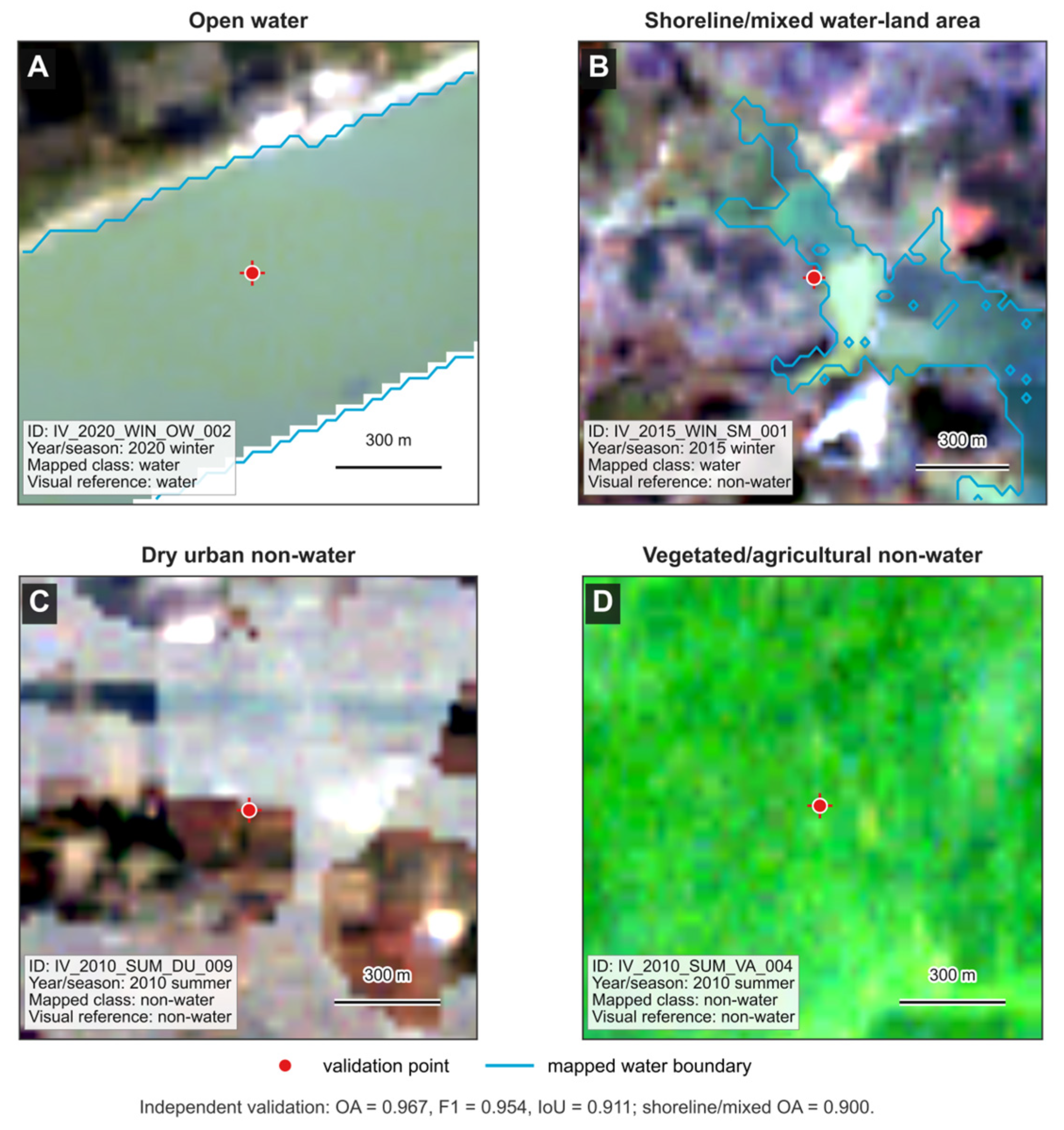
Because JRC-related layers were also used in the water-mapping workflow, the JRC comparison was not treated as a fully independent accuracy assessment. An additional visual interpretation check was therefore conducted using the Landsat seasonal composites, with Google Earth and QGIS inspection used as auxiliary visual references. A total of 480 validation points were selected across the six benchmark years and two seasons, with 40 points assigned to each year–season combination. To cover both clear and difficult interpretation settings, samples were stratified across four validation contexts: open water, shoreline/mixed water–land areas, dry urban non-water area, and vegetated/agricultural non-water areas. These contexts were used only for sampling and visual interpretation; the final reference labels were binary water/non-water labels. The manual reference labels were compared with the mapped water classes using a confusion matrix, and overall accuracy, precision, recall, F1, and IoU were calculated.

After classification, the seasonal water masks were refined to reduce isolated misclassified patches, low-valid-count artifacts, and period-specific mapping errors. These refinements were used to improve the spatial and temporal coherence of major rivers, lakes, and seasonal shoreline patterns. To examine whether the final mask refinements affected the statistical results, key models were repeated using the pre-refinement water product. This comparison was used as a stability check for the main water–LST associations.

Auxiliary variables included NDVI, built-up fraction, elevation, and slope. The built-up fraction was derived from the GHSL built-up surface product, and terrain variables were derived from SRTM elevation data [33,34]. All products were harmonized to the 250 m analytical grid before regression, spatial prediction, city heterogeneity, and robustness analyses.

2.3. Analytical Grid and Multiscale Water-Fraction Measurement

For each 250 m × 250 m analytical grid cell, surface-water fraction was calculated from the 30 m water mask as the proportion of water pixels within the cell. To describe the surrounding landscape context, surface-water fraction was further calculated within square windows centered on each grid-cell centroid, with side lengths of 500, 750, 1000, 1250, 1500, 1750, and 2000 m. Together, these measures represent the surface-water fraction from the cell scale to broader neighborhood scales.

For windows crossing the outer boundary of the study area, only pixels inside the nine-city boundary were included. Each water-fraction measure was paired with the same LST value for the corresponding grid cell and period. This provided a consistent basis for comparing water–LST associations across measurement scales.

Larger windows include more of the surrounding land-cover context, such as nearby rivers, lakes, shorelines, vegetation, built-up surfaces, and terrain. The multiscale comparison was therefore used to examine whether LST was more closely associated with immediate water coverage or with broader landscape context.

The balanced sample described in Section 2.1 was used in all main associations, within–between, grid fixed-effect, spatial prediction, city-specific, and leave-one-city-out analyses. Model covariates included surface-water fraction, NDVI, built-up fraction, elevation, and slope. Continuous variables were standardized to improve comparability across models. Seasonal association models included year fixed effects, and standard errors were clustered by grid cell unless otherwise specified.

2.4. Seasonal Association and Within–Between Models

Seasonal water–LST associations were estimated separately for summer and winter at each measurement scale. The baseline model controlled for vegetation, built-up fraction, elevation, slope, and benchmark-year fixed effects:

$${\mathrm{L}\mathrm{S}\mathrm{T}}_{iy}={\beta }_0+{\beta }_1{W}_{iy}^s+{\gamma }^{\prime }{X}_{iy}+{\delta }_y+{\epsilon }_{iy}$$

(1)

where ${\mathrm{L}\mathrm{S}\mathrm{T}}_{iy}$ is daytime land surface temperature for grid cell $i$ in benchmark year $y$, $W_{iy}^s$ is surface-water fraction at measurement scale $s$, $X_{iy}$ includes NDVI, built-up fraction, elevation, and slope, and ${\delta }_y$ denotes benchmark-year fixed effects. The raw coefficient ${\beta }_1$ is reported in °C per unit increase in surface-water fraction. Standardized coefficients were also estimated within each seasonal sample to compare association strength across measurement scales.

To compare the water–LST slope between summer and winter, a pooled seasonal interaction model was estimated:

$${\mathrm{L}\mathrm{S}\mathrm{T}}_{iy}={\beta }_0+{\beta }_1{W}_{iy}^s+{\beta }_2{\mathrm{W}\mathrm{i}\mathrm{n}\mathrm{t}\mathrm{e}\mathrm{r}}_{iy}+{\beta }_3\left(W_{iy}^s\times {\mathrm{W}\mathrm{i}\mathrm{n}\mathrm{t}\mathrm{e}\mathrm{r}}_{iy}\right)+{\gamma }^{\prime }{X}_{iy}+{\delta }_y+{\epsilon }_{iy}$$

(2)

Here, ${\mathrm{W}\mathrm{i}\mathrm{n}\mathrm{t}\mathrm{e}\mathrm{r}}_{iy}$ equals 1 for winter observations and 0 for summer observations. The coefficient ${\beta }_1$ represents the summer water–LST slope, and ${\beta }_3$ represents the winter-minus-summer difference in that slope. The winter slope is therefore ${\beta }_{1 }+{\beta }_3$. This model was used to compare seasonal differences in raw temperature-unit coefficients, while the season-specific standardized models were used to compare relative association strength within each season.

To distinguish persistent spatial differences from changes within the same location over time, surface-water fraction was decomposed into a grid-cell mean and a temporal deviation from that mean [24,25]:

$${\mathrm{L}\mathrm{S}\mathrm{T}}_{iy}={\beta }_0+{\beta }^B{\overline{W}}_i^s+{\beta }^W\left(W_{iy}^s-{\overline{W}}_i^s\right)+{\gamma }^{\prime }{X}_{iy}+{\delta }_y+{\epsilon }_{iy}$$

(3)

In this model, ${\overline{W}}_i^s$ is the mean surface-water fraction of grid cell $i$ across the corresponding seasonal periods. The between coefficient ${\beta }^B$ describes differences among grid cells with different long-term water contexts, whereas the within coefficient ${\beta }^W$ describes deviations from a grid cell’s own average water condition. The difference between ${\beta }^B$ and ${\beta }^W$ was evaluated using a Wald linear contrast. Grid fixed-effect models with the same sample and controls were also estimated to examine within-location associations after absorbing time-invariant grid-cell characteristics.

2.5. Spatial Consistency and Cross-City Assessment

The spatial consistency of the water–LST relationship was examined after the main seasonal models were established. First, blocked spatial validation was used to test whether the fitted relationships remained informative in areas that were not used for model fitting [26,27]. The study area was divided into 5 km and 10 km spatial blocks, and observations from the same grid cell were assigned to the same validation fold. This block-based validation provided a more conservative assessment of model transferability across areas with different thermal and land-cover conditions.

Model performance was assessed using RMSE, MAE, and R². The interpretation gives priority to RMSE from the 10 km block validation because this setting provides the stricter test of spatial transferability. Results from the 5 km validation and from MAE and R² were used to check whether the same pattern was retained. Adjacent measurement supports were then compared to avoid treating very small differences as meaningful scale effects. In summer, the representative 500 m support was compared with 250, 750, and 1000 m; in winter, the representative 2000 m support was compared with 1750, 1500, and 1250 m. For each pair of supports, we compared the absolute standardized water coefficient and 10 km RMSE.

City-level variation was then examined by fitting the same seasonal association models separately for the nine municipalities. This analysis was used to compare whether the direction and magnitude of the water–LST relationship changed across different hydrological and urban settings.

Finally, leave-one-city-out validation was used to assess cross-city transferability. In each run, observations from eight municipalities were used for model fitting, and the remaining municipality was used for evaluation.

2.6. Built-Up Context and Robustness Analyses

Built-up context was assessed by adding interaction terms between surface-water fraction and built-up fraction at selected measurement supports. Models were estimated for the full sample and for the subset of grid cells with nonzero built-up fraction, allowing the interaction to be compared between the regional sample and developed settings.

Several sensitivity analyses were used to examine the stability of the main water–LST relationship. Native-resolution MODIS LST was used as an alternative thermal response to test whether the negative association was retained without 250 m RF downscaling. RF-A and RF-B LST products were then compared to examine whether including water-sensitive predictors during downscaling changed the estimated water–LST association. Residual spatial autocorrelation was evaluated using Moran’s I [35], and spatial-error models were estimated on period-by-5 km block aggregates using a row-standardized, period-specific four-neighbor rook-style spatial-weights matrix [36]. The weights linked adjacent 5 km blocks sharing horizontal or vertical grid edges within the same period, with no cross-period links. These models used the same seasonal response, 1500 m water-fraction support, covariates, and period fixed effects as the corresponding block-level OLS models and were used to examine whether accounting for residual spatial dependence changed the direction and magnitude of the water–LST coefficients. Random-forest/SHAP diagnostics were used as supplementary predictive evidence for nonlinear response patterns [37]. Key models were also repeated using the pre-refinement water product to evaluate the influence of water-mask construction. Threshold sensitivity was examined by repeating the water-mask generation, multiscale water-fraction calculation, and seasonal association models under alternative seasonal probability thresholds. Summer thresholds of 0.45, 0.48, 0.50, and 0.55 and winter thresholds of 0.95, 0.97, and 0.99 were tested, while the classifier, input imagery, study boundary, covariates, sample, and model structure were kept unchanged.

Table 2. Empirical questions, analytical approaches, and main outputs.

Empirical Question	Analytical Approach	Main Output
Seasonal scale dependence	Season-specific OLS models by measurement scale	Standardized water coefficients and 95% confidence intervals
Seasonal difference in raw slope	Pooled water × winter interaction model	Winter-minus-summer difference in °C per unit water fraction
Spatial versus temporal structure	Within–between model and grid fixed-effect model	Between and within coefficients, Wald contrast, and fixed-effect estimates
Spatial prediction	5 km and 10 km blocked spatial cross-validation	Held-out RMSE, MAE, R2, and support-specific prediction performance
Cross-city transferability	Leave-one-city-out validation	Held-out city RMSE by season and measurement scale
Built-up context and robustness	Built-up interactions and sensitivity analyses	Robustness of water–LST associations across alternative model and data specifications

summarizes the analytical framework.

3. Results

3.1. Remote-Sensing Product Consistency and Seasonal Surface-Water Patterns

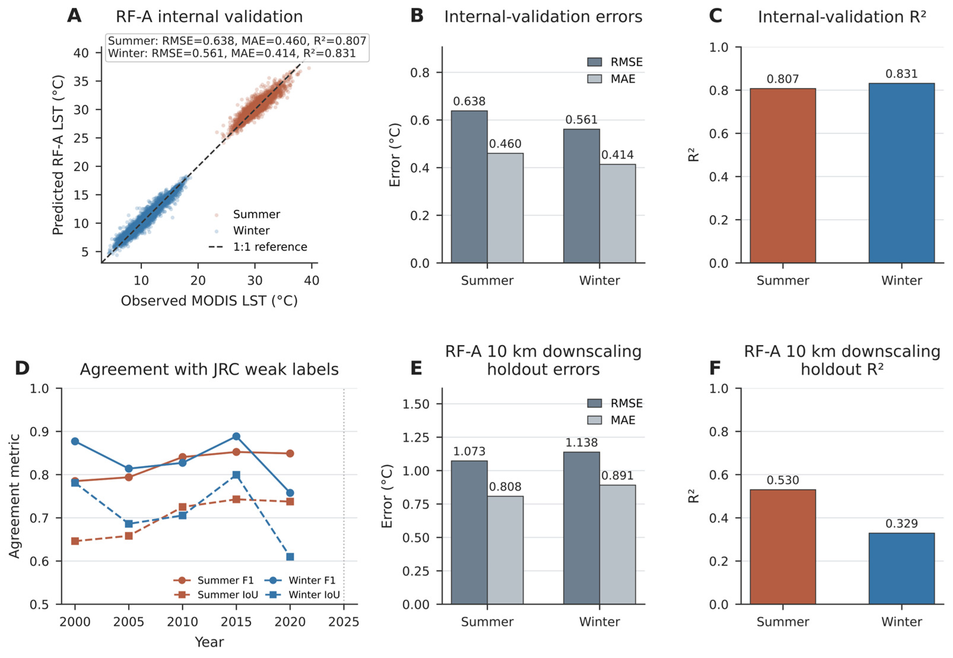
The RF-A downscaled LST product showed consistent performance across the seasonal composites. Mean internal-validation RMSE values were 0.638 °C in summer and 0.561 °C in winter, with corresponding R² values of 0.807 and 0.831. In the 10 km spatial holdout, RMSE values were 1.073 °C in summer and 1.138 °C in winter. These results indicate that the downscaled product reproduced the main seasonal LST patterns of the Wuhan Urban Agglomeration and provided a consistent thermal dataset for the multiscale analysis (Figure 2).

The surface-water product showed coherent seasonal patterns. Agreement with the JRC MonthlyHistory weak labels was moderate to high during the overlapping periods, with mean F1 values of 0.824 in summer and 0.833 in winter, and mean IoU values of 0.702 and 0.716, respectively. These values were interpreted as consistency evidence rather than as an independent accuracy assessment because JRC-related layers were also used in the mapping workflow, and the monthly JRC records were not available for the 2025 composites.

The independent visual interpretation check provided a separate point-based assessment of the seasonal water masks. Across 480 samples stratified by year, season, and validation context, the mapped water product achieved an overall accuracy of 0.967, precision of 0.932, recall of 0.976, F1 of 0.954, and IoU of 0.911 (Table 3). The confusion matrix included 164 correctly mapped water samples, 300 correctly mapped non-water samples, 12 false positives, and 4 false negatives. Accuracy was similar between summer and winter, with OA values of 0.963 and 0.971, respectively. Disagreement was concentrated mainly in shoreline and mixed water–land contexts, where OA decreased to 0.900.

Table 3. Independent visual validation of the seasonal surface-water product.

Visual Reference Label	Mapped Water	Mapped Non-Water	Total
water	164	4	168
non-water	12	300	312
Total	176	304	480

Note: Rows represent visual reference labels, and columns represent mapped classes. Overall accuracy = 0.967, precision = 0.932, recall = 0.976, F1 = 0.954, and IoU = 0.911. Seasonal OA was 0.963 in summer and 0.971 in winter; shoreline/mixed OA was 0.900. Representative examples are shown in Figure 3.

Table 3. Independent visual validation of the seasonal surface-water product.

Visual Reference Label	Mapped Water	Mapped Non-Water	Total
water	164	4	168
non-water	12	300	312
Total	176	304	480

Note: Rows represent visual reference labels, and columns represent mapped classes. Overall accuracy = 0.967, precision = 0.932, recall = 0.976, F1 = 0.954, and IoU = 0.911. Seasonal OA was 0.963 in summer and 0.971 in winter; shoreline/mixed OA was 0.900. Representative examples are shown in Figure 3.

Figure 3. Representative samples used for independent visual validation of the seasonal surface-water product. Panels show examples of (A) open water, (B) shoreline/mixed water–land area, (C) dry urban non-water area, and (D) vegetated/agricultural non-water area. Background colors represent the Landsat seasonal composites used for visual interpretation. Blue outlines indicate mapped water boundaries, and red points indicate validation samples. Mapped class refers to the surface-water product, and visual reference refers to manual interpretation.

Figure 3. Representative samples used for independent visual validation of the seasonal surface-water product. Panels show examples of (A) open water, (B) shoreline/mixed water–land area, (C) dry urban non-water area, and (D) vegetated/agricultural non-water area. Background colors represent the Landsat seasonal composites used for visual interpretation. Blue outlines indicate mapped water boundaries, and red points indicate validation samples. Mapped class refers to the surface-water product, and visual reference refers to manual interpretation.

At the regional scale, the resulting maps showed the main hydrological structure of the Wuhan Urban Agglomeration, including the Yangtze River corridor and major lake clusters. Surface-water coverage was more extensive and spatially continuous in lake- and river-connected areas around Wuhan, Ezhou, and Huangshi, whereas several inland municipalities showed lower and more fragmented water coverage. These spatial contrasts provided the basis for comparing the water–LST relationship across broad regional differences and repeated observations within the same locations.

3.2. Seasonal and Multiscale Water–LST Associations

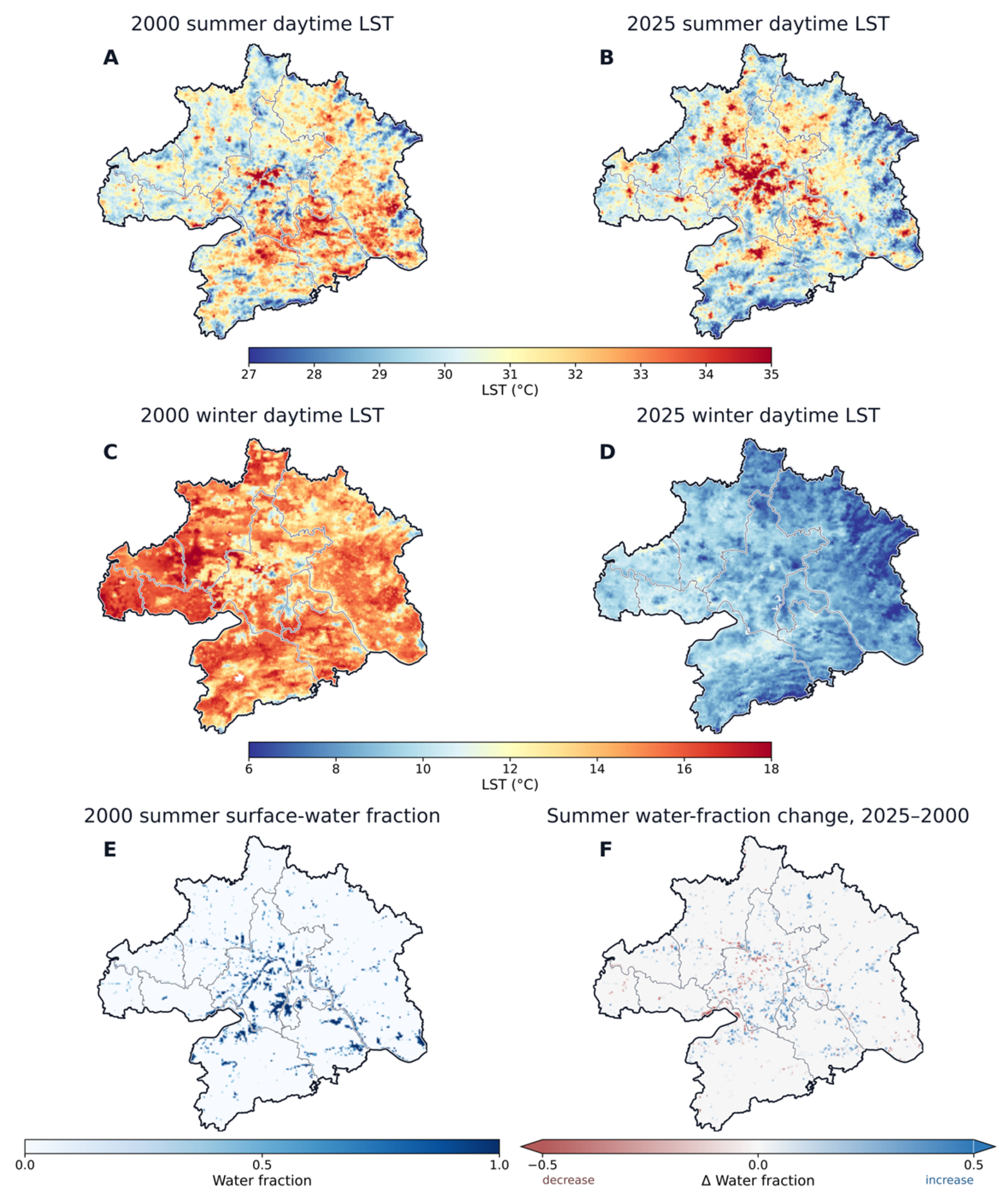
Surface-water fraction was negatively associated with daytime LST in both summer and winter. This relationship was observed for the cell-internal measure and for all surrounding-window measures, indicating that areas with a higher proportion of surface water generally had lower daytime surface temperatures. Figure 4 shows representative seasonal spatial patterns of daytime LST and surface-water fraction.

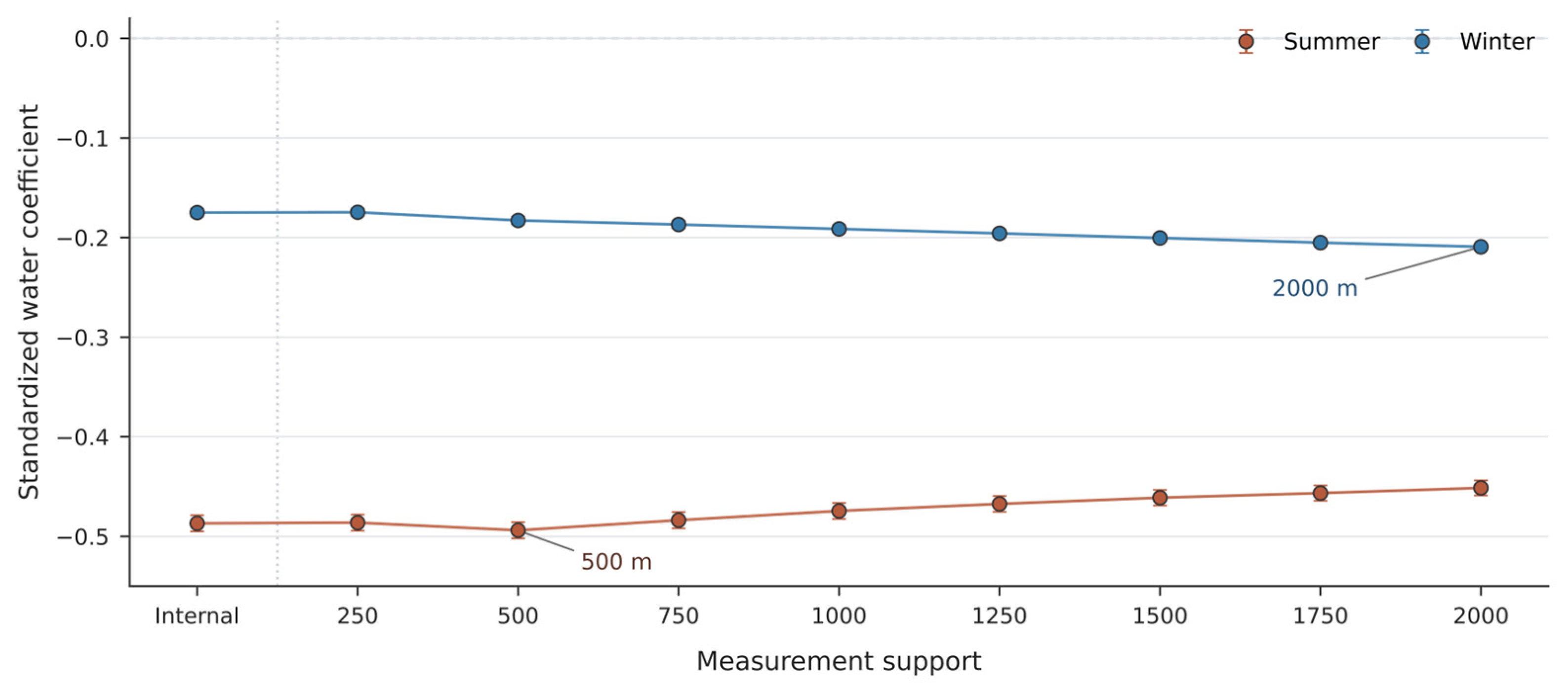
The scale-response pattern differed clearly between the two seasons. In summer, the strongest standardized association within the tested supports occurred at 500 m ($\beta$ = −0.494, 95% CI −0.502 to −0.486). The coefficients remained negative at broader supports, but the association weakened slightly after the 500 m scale. This pattern suggests that summer LST was more closely associated with water coverage in the nearby landscape than with either the individual grid cell or broader surrounding supports.

In winter, the standardized association strengthened toward broader supports, with the largest value occurring at 2000 m within the tested range ($\beta$ = −0.209, 95% CI −0.213 to −0.206). Compared with summer, the winter relationship was less concentrated at the local-neighborhood scale and was more closely aligned with the wider distribution of rivers, lakes, and surrounding land cover.

The seasonal comparison also differed between standardized and raw temperature-unit coefficients. The standardized models indicated that the relative water–LST association was strongest in summer, with the largest coefficient at 500 m. In the pooled raw-coefficient model, however, the broader winter support showed a more negative temperature-unit slope. At the 2000 m support, the winter-minus-summer difference was −0.781 °C per unit increase in water fraction, equivalent to −0.078 °C per 0.1 increase in water fraction.

Standardized and raw coefficients emphasize different aspects of the water–LST relationship. Standardized coefficients describe the relative strength of the association within each seasonal sample, whereas raw coefficients retain the temperature-unit slope. Summer therefore showed a stronger relative association with water fraction, while winter showed a steeper °C-per-fraction slope at the broadest tested support. The seasonal scale-response patterns are shown in Figure 5.

3.3. Spatial Context and Within-Location Variation in the Water–LST Relationship

The water–LST relationship was mainly shaped by regional spatial contrasts. Grid cells located in lake-rich and river-connected settings generally showed lower daytime LST than areas with less surrounding water. This spatial contrast was much stronger than the LST differences associated with seasonal water-fraction changes within the same grid cells.

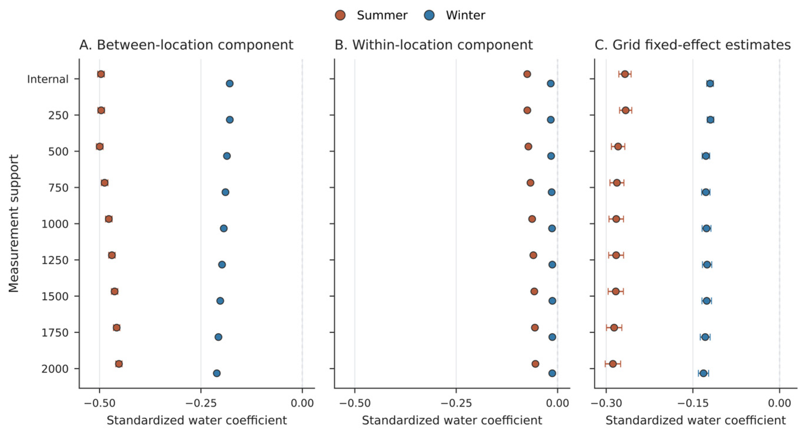
At the 1500 m support, the standardized summer coefficient for the spatial component was −0.463 (95% CI −0.471 to −0.455), while the coefficient for within-location variation was −0.057 (95% CI −0.060 to −0.055). The difference between the two components was −0.405 (95% CI −0.413 to −0.398, p < 0.001). The same pattern appeared in winter. The spatial component was −0.202 (95% CI −0.206 to −0.199), whereas the within-location component was −0.013 (95% CI −0.014 to −0.012), with a difference of −0.190 (95% CI −0.193 to −0.186, p < 0.001).

The grid fixed-effect estimates were also negative, with values of −0.283 in summer and −0.126 in winter. This result indicates that increases in water fraction within the same grid cell were still associated with lower LST, although the magnitude was smaller than the regional spatial contrast.

Overall, the results show that the observed water–LST association was dominated by stable spatial context. Persistent lakes, river corridors, and surrounding blue-green landscapes contributed to clear thermal differences among locations, while seasonal water-fraction deviations within individual grid cells produced weaker but still negative associations. The spatial and within-location components across measurement supports are shown in Figure 6.

3.4. Spatial Consistency of the Water–LST Relationship Across Cities

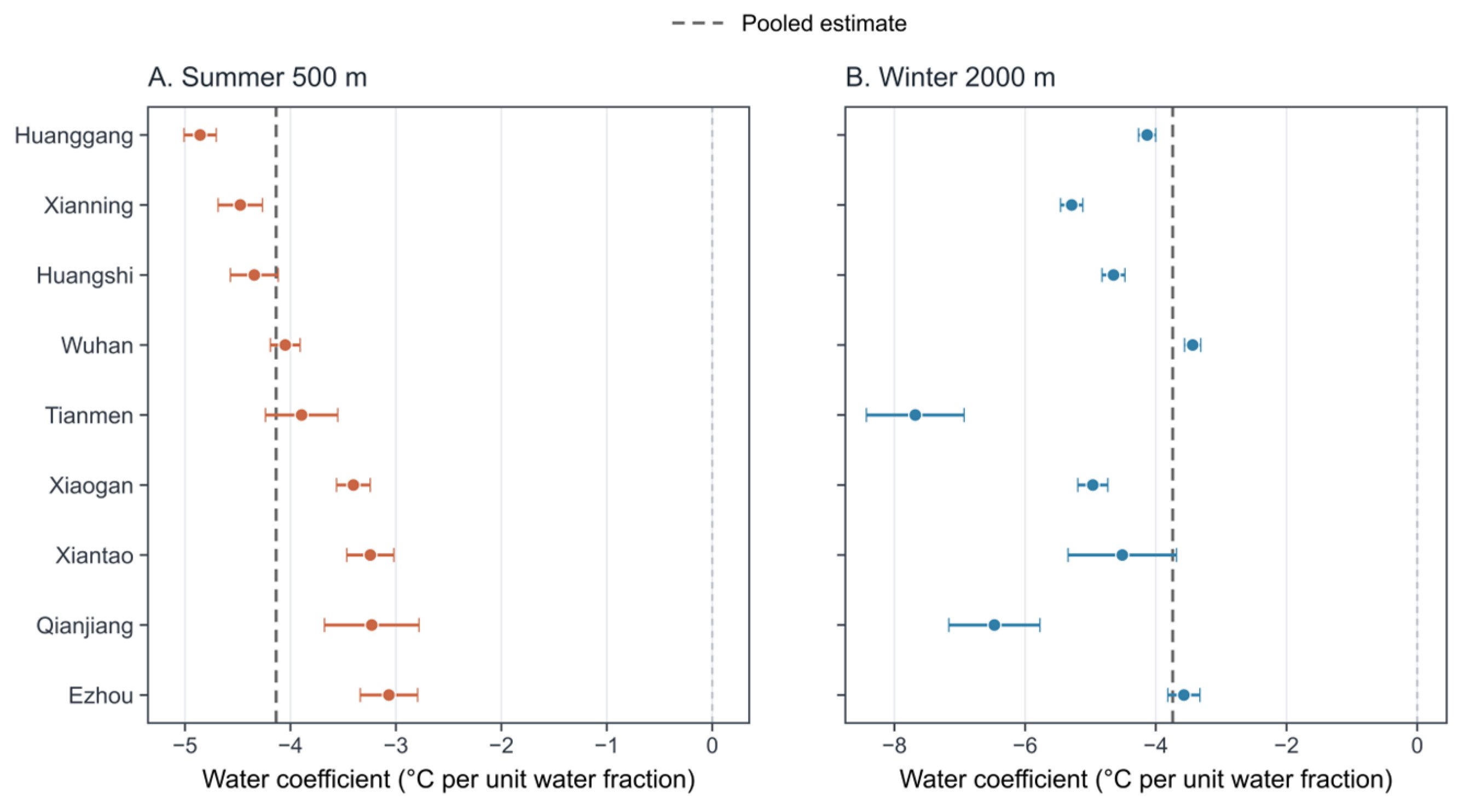
The negative water–LST relationship was broadly consistent across the Wuhan Urban Agglomeration, but its strength varied among cities and seasons. At the representative seasonal supports, all city-specific coefficients were negative. In summer, the 500 m coefficients ranged from −4.856 to −3.066 °C per unit increase in water fraction. In winter, the 2000 m coefficients ranged from −7.681 to −3.436 °C per unit increase in water fraction. This indicates that the cooling-related association of surface water was not limited to a single municipality, although its magnitude differed across local hydrological and urban settings. The city-specific coefficients at the representative seasonal supports are shown in Figure 7.

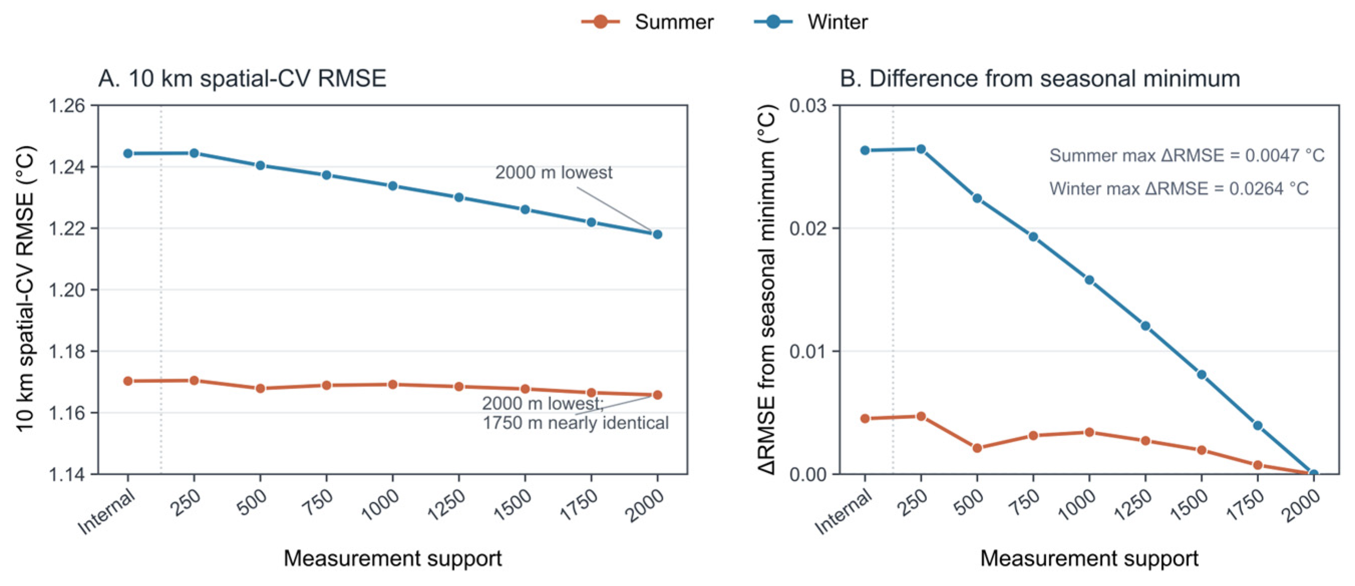
The spatial-validation results showed that these relationships remained useful when applied to areas outside the fitting locations. In summer, prediction accuracy changed only slightly across measurement supports. The lowest 10 km spatial-validation RMSE occurred at 2000 m (1.166 °C), followed by 1750 m (1.167 °C), but the difference was only 0.0007 °C. This near-equivalence suggests that several water-fraction supports captured similar regional thermal information in summer, even though the strongest association appeared at 500 m.

Winter showed a clearer broad-scale pattern. The 2000 m support produced the lowest 10 km spatial-validation RMSE (1.218 °C), followed by 1750 m (1.222 °C). This result was consistent with the winter scale-response pattern in Section 3.2, where broader water and landscape conditions were more closely associated with LST. The 5 km validation showed the same broad pattern, with the 2000 m support producing the lowest RMSE and MAE and the highest R² in both seasons. The multiscale spatial cross-validation results are shown in Figure 8.

The neighboring-support comparison further showed that the representative supports should be interpreted as peak supports within the tested range rather than sharply defined optimal distances. In summer, the 500 m support had a stronger standardized association than the adjacent 250, 750, and 1000 m supports, but the 10 km spatial-validation RMSE differences were very small, ranging from 0.0010 to 0.0026 °C (

Table 4. Neighboring-support comparison for the representative seasonal supports.

Season	Comparison	Δ Standardized Coefficient	Δ 10 km RMSE (°C)
Summer	500 m vs. 250 m	0.0077	0.0026
Summer	500 m vs. 750 m	0.0101	0.0010
Summer	500 m vs. 1000 m	0.0194	0.0013
Winter	2000 m vs. 1750 m	0.0042	0.0040
Winter	2000 m vs. 1500 m	0.0088	0.0081
Winter	2000 m vs. 1250 m	0.0134	0.0121

Note: Positive values indicate that the representative support had a larger absolute standardized water coefficient or lower 10 km RMSE than the comparison support.

). This indicates that 500 m represented the summer association peak, whereas nearby supports provided similar spatial-prediction performance. In winter, the 2000 m support was very close to 1750 m but showed clearer separation from 1500 and 1250 m. These results support a broad-scale winter pattern rather than a sharply defined 2000 m threshold.

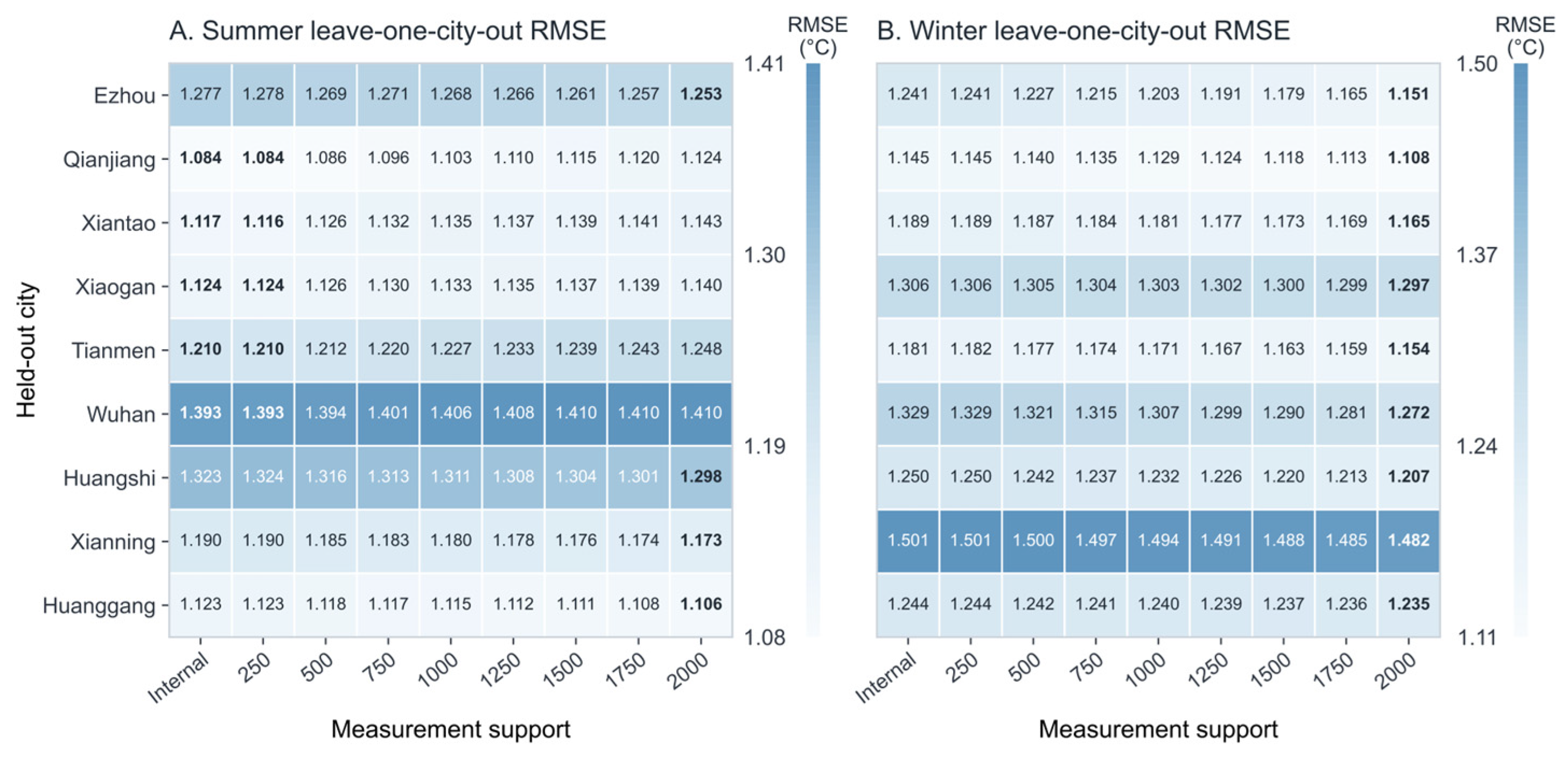
The leave-one-city-out results further confirmed the seasonal contrast (Figure 9). In summer, the mean held-out RMSE was almost the same for the 500 m and cell-internal supports, with values of 1.2038 °C and 1.2044 °C, respectively. In winter, the lowest mean held-out RMSE occurred at 2000 m (1.230 °C), followed by 1750 m (1.235 °C). Wuhan had the largest summer prediction error, whereas Xianning had the largest winter prediction error, suggesting that local thermal background, hydrological structure, and urban form still influenced cross-city performance.

Overall, the water–LST relationship showed a stable negative direction across cities, but the scale-response pattern changed with season and analytical purpose. Summer results emphasized nearby water and shoreline context for association strength, while prediction differences among scales were small. Winter results more consistently favored broader landscape supports. These findings indicate that scale selection should be linked to the seasonal thermal pattern being examined rather than treated as a fixed distance.

3.5. Built-Up Context and Stability of the Water–LST Relationship

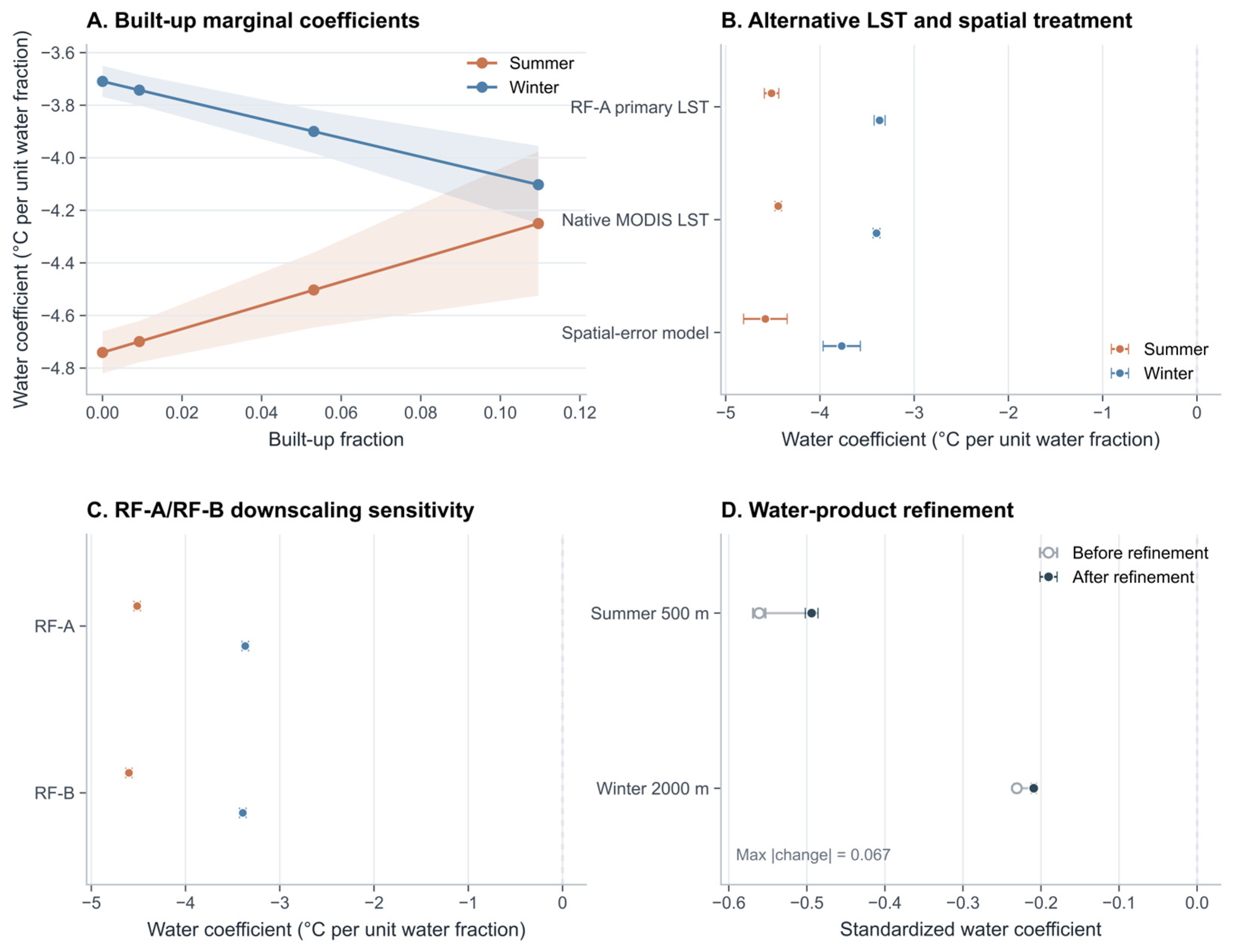
Built-up intensity modified the water–LST relationship, but this effect was secondary to the seasonal and scale-dependent patterns reported above. At the 2000 m support, the summer water × built-up interaction was positive in the full sample (0.248, p < 0.001), indicating that the negative association between surface-water fraction and LST became slightly weaker as the built-up fraction increased. The same direction was observed after the analysis was restricted to grid cells with built-up land (0.192, p < 0.001), suggesting a relatively stable summer pattern within built-up settings.

The winter interaction was less consistent. In the full sample, the water × built-up interaction was negative (−0.199, p < 0.001), but this relationship was not evident in the positive-built-up subset (−0.048, p = 0.198). This contrast indicates that the winter interaction was more strongly influenced by differences between built and non-built landscapes. Built-up modification was therefore clearer in summer than in winter.

The negative water–LST relationship was retained under alternative thermal-response settings. When native-resolution MODIS LST was used instead of the 250 m downscaled product, the 1500 m water coefficients remained negative in both summer (−4.443) and winter (−3.400). The RF-A/RF-B comparison showed a similar pattern. After water-sensitive predictors were included in the downscaling model, the 1500 m coefficients changed only slightly, from −4.513 to −4.601 in summer and from −3.367 to −3.392 in winter. These results indicate that the main negative association was not dependent on a single downscaled LST product.

The spatial-error models also produced negative water coefficients, with values of −4.579 in summer and −3.769 in winter at the 1500 m support. Compared with the corresponding block-level OLS models, residual Moran’s I decreased from 0.647 to −0.054 in summer and from 0.712 to −0.036 in winter (

Table 5. Comparison between block-level OLS and spatial-error models.

Season	Model	Water Coefficient	Standard Error	p Value	Residual Moran’s I
Summer	OLS	−5.455	0.093	<0.001	0.647
Summer	SEM	−4.579	0.118	<0.001	−0.054
Winter	OLS	−4.319	0.101	<0.001	0.712
Winter	SEM	−3.769	0.101	<0.001	−0.036

Note: Both models were estimated on period-by-5 km block aggregates at the 1500 m water-fraction support. The SEM used a row-standardized, period-specific four-neighbor rook-style spatial-weights matrix. p values reported as 0 in the model output are shown as <0.001.

). This indicates that spatial dependence strongly affected the residual structure, but accounting for it did not change the direction of the main water–LST association.

Water-product refinement affected coefficient magnitude but did not change the main direction of the results. The largest absolute change in a standardized total-association coefficient was 0.067. The summer 500 m coefficient changed from −0.561 before refinement to −0.494 after refinement, and the winter 2000 m coefficient changed from −0.231 to −0.209. The same negative direction was retained for both the spatial and within-location components, although the smaller within-location estimates were more sensitive to water-product construction. The built-up context and main robustness results are summarized in Figure 10.

The threshold tests showed a similar pattern (

Table 6. Threshold sensitivity of seasonal water classification and water–LST associations.

Season	Threshold	Water Coefficient	Standardized Coefficient	Peak Support
Summer	0.45	−4.500	−0.564	500 m
Summer	0.48	−4.570	−0.567	500 m
Summer	0.50	−4.590	−0.568	500 m
Summer	0.55	−4.664	−0.570	500 m
Winter	0.95	−3.857	−0.249	2000 m
Winter	0.97	−3.934	−0.247	2000 m
Winter	0.99	−4.068	−0.238	2000 m

Note: Coefficients are reported at the representative seasonal supports: 500 m for summer and 2000 m for winter. Peak support indicates the largest absolute standardized water coefficient. All other model settings were kept unchanged.

). When the summer probability threshold was changed from 0.45 to 0.55, the 500 m water coefficient remained negative, ranging from −4.500 to −4.664 °C per unit increase in water fraction. The strongest standardized association also remained at 500 m. In winter, the 2000 m coefficients remained negative under thresholds of 0.95, 0.97, and 0.99, ranging from −3.857 to −4.068 °C per unit increase in water fraction. The strongest standardized association remained at 2000 m. These results suggest that the selected seasonal thresholds affected coefficient magnitude slightly but did not change the direction of the water–LST relationship or the main seasonal scale-response pattern.

4. Discussion

4.1. Seasonal Differences in the Water–LST Relationship

Surface-water fraction was negatively associated with daytime LST in both summer and winter. This pattern is consistent with the general thermal behavior of water bodies in urban environments. Compared with impervious and other non-water surfaces, water surfaces may warm more slowly during the day because of their higher heat capacity, while evaporation can consume part of the available energy. These processes provide a plausible explanation for the lower daytime LST observed in areas with higher surface-water fraction, although they were not directly measured in this study [4,7,11].

The summer association was strongest at 500 m. This suggests that summer LST was closely related to the immediate environment around water bodies. Under strong solar radiation, impervious surfaces heat rapidly, while open water, moist shorelines, and nearby vegetation may slow daytime warming through evaporation, shading, and higher surface moisture. The thermal contrast is therefore most visible where water bodies meet surrounding land, especially along shorelines and in mixed blue–green–built-up environments. In this sense, the 500 m result highlights the role of nearby water and shoreline conditions in shaping summer surface temperature [11,18].

Winter showed a broader scale pattern, with the association strengthening toward 2000 m. This may be because the local contrast between water and land becomes weaker under lower radiation and reduced evaporation. Under these conditions, large lakes and connected rivers may be more closely associated with LST through thermal inertia and the surrounding blue–green landscape than through immediate shoreline cooling.

Overall, the seasonal contrast suggests that summer LST was mainly shaped by nearby shoreline and land-cover conditions, whereas winter LST was more closely related to larger water systems and the surrounding blue–green landscape. This helps explain why the strongest association occurred at 500 m in summer but shifted toward 2000 m in winter.

4.2. Spatial Context as the Main Source of the Observed Relationship

The results show that the regional water–LST relationship was mainly shaped by persistent differences among places. In the Wuhan Urban Agglomeration, areas with high water fractions are usually connected with large lakes, river corridors, wetland margins, and surrounding blue–green spaces. These areas differ from inland built-up areas not only in water coverage but also in vegetation, impervious surface intensity, terrain, shoreline conditions, and urban development pattern. Such combined landscape conditions help explain why water-rich areas generally showed lower daytime LST [19,21,38,39].

This pattern is consistent with previous studies showing that the thermal influence of urban water bodies depends strongly on their surrounding land-cover context. Large lakes and rivers may be associated with lower surface warming because of high heat capacity, evaporation, shoreline moisture, and adjacent vegetation. Lower built-up intensity and stronger blue–green connectivity around water bodies may further reinforce the cool-surface pattern. Therefore, the lower LST observed in water-rich areas is likely related to the combined thermal influence of water bodies, shorelines, vegetation, and surrounding land-cover conditions [7,16,17].

The weaker within-location relationship provides a useful contrast. Changes in water fraction within the same grid cell were also associated with lower LST, but their magnitude was much smaller than the regional contrast between water-rich and water-poor locations. This is reasonable because same-cell changes are often related to shoreline movement, seasonal water-level variation, small ponds, or mixed pixels. These local changes may influence surface temperature, but they do not usually represent the broader lake–river–vegetation setting that distinguishes water-rich areas from inland built-up areas [24,25].

4.3. Scale Interpretation and Cross-City Differences

The multiscale results suggest that the meaning of surface-water fraction changes with the measurement support. In summer, the strongest standardized association occurred at 500 m, indicating that daytime LST was more closely related to water coverage in the nearby landscape than to water coverage within the individual grid cell alone. This support may better represent the combined thermal setting of open water, shorelines, riparian vegetation, and adjacent built-up surfaces. The small prediction differences among nearby supports also suggest that this scale should be interpreted as part of a nearby landscape response rather than as a sharply defined distance.

Winter showed a broader-scale pattern. The association strengthened toward 2000 m and remained consistent in spatial validation and cross-city testing. This may reflect the weaker daytime radiation, different vegetation conditions, and larger seasonal influence of major lakes, river corridors, and surrounding blue–green landscapes in winter. Under these conditions, water fraction measured over a broader landscape support may better describe regional thermal contrasts than a more localized measure.

The city-level results further indicate that the negative water–LST association was widespread across the urban agglomeration but varied in magnitude among municipalities. This variation is expected because the nine cities differ in lake density, river networks, terrain, urban development intensity, and surrounding land-cover composition. In cities with large lakes and connected river systems, surface-water fraction may represent broader blue–green landscape structure, whereas in more inland or fragmented settings it may describe smaller and more localized water features.

Overall, these findings show that surface-water fraction is not a scale-invariant indicator of urban thermal conditions. Its association with daytime LST depends on season, measurement support, and local hydrological–urban context. For multi-city urban thermal studies, scale selection should therefore be linked to the seasonal setting and the spatial structure of water bodies rather than treated as a fixed methodological choice.

4.4. Built-Up Context and Sensitivity of the Main Pattern

Built-up intensity changed the strength of the water–LST relationship, but it was not the main source of the seasonal and scale-dependent patterns. In summer, the negative association between surface-water fraction and LST became slightly weaker as the built-up fraction increased. This suggests that dense urban surroundings may reduce the thermal contrast associated with nearby water bodies. Highly built-up areas often contain more heat-retaining surfaces, less natural shoreline vegetation, and more fragmented blue–green space, which can weaken the cool-surface pattern around water [16,40,41].

The winter pattern was less clear. The interaction appeared in the full sample but was not evident after the analysis was restricted to grid cells with built-up land. This suggests that the winter result was partly shaped by broader differences between built and non-built landscapes. Built-up fraction is therefore better understood as a general indicator of urban background conditions. It cannot fully represent building height, street geometry, shading, ventilation, shoreline design, or anthropogenic heat [40,41,42].

The robustness analyses supported the stability of the negative water–LST association. The pattern was retained when native MODIS LST was used, when the RF-A and RF-B LST products were compared, and when residual spatial dependence was addressed using spatial-error models. The spatial-error models reduced residual Moran’s I while keeping negative water coefficients in both seasons, indicating that spatial dependence affected model diagnostics but did not change the direction of the main relationship. Because OLS and spatial-error models treat spatial structure differently, the comparison was used as a sensitivity analysis. Taken together, these results suggest that the main interpretation is supported by the direction, magnitude, and consistency of coefficients across alternative data and model specifications.

Water-product refinement mainly affected the strength of the estimated relationship. This is expected in lake- and river-rich landscapes, where shoreline position, seasonal water levels, cloud-free observations, and mixed pixels can influence mapped water fraction. These effects were more visible for same-cell water changes because local changes in water fraction were relatively small. In contrast, the broad difference between lake-rich and inland areas was more stable.

4.5. Implications for Land-Cover-Based Thermal Assessment and Future Research

These results suggest that surface-water fraction is a seasonal and scale-dependent indicator of urban thermal conditions. In summer, the association was strongest at the nearby landscape support, indicating that shoreline zones and adjacent land cover were closely related to daytime LST. In this setting, water area, riparian vegetation, impervious surfaces, and local blue-green continuity may jointly shape the observed thermal pattern. In winter, the broader-support association suggests that large lakes, river corridors, wetlands, and connected open spaces were more relevant to regional thermal contrasts [1,2,3]. These findings highlight the need to match the measurement support of surface-water indicators with the seasonal and spatial context of the study area.

The results also caution against using a single buffer distance to represent the thermal role of urban water bodies. In land-cover-based thermal assessment, the appropriate measurement support depends on the season, the spatial scale of analysis, and the surrounding urban context. Local shoreline composition may be more relevant for summer daytime LST, whereas broader river–lake systems and blue–green landscape structure may better describe winter and regional-scale patterns.

Several limitations should be considered when applying these findings. LST describes the radiometric surface condition and cannot directly represent near-surface air temperature, thermal comfort, or human heat exposure [3,8]. The downscaled LST product was evaluated through MODIS-scale consistency and spatial holdout tests, but independent fine-resolution thermal observations were not available. The thermal response also has a scale limitation. Although the analysis was conducted on a 250 m grid, the parent MODIS LST product has an approximately 1 km spatial support. Narrow canals, small ponds, fragmented shorelines, street-canyon geometry, building shadows, and micro-scale ventilation conditions could not be fully resolved. In addition, the 30 m Landsat water maps describe water distribution at a finer spatial resolution than the thermal response. The JRC comparison provided useful consistency evidence for the mapped water product, and the added visual interpretation check provided an independent assessment across all six benchmark years and two seasons. However, some uncertainty remains in shoreline and mixed water–land pixels, where seasonal water-level changes, aquatic vegetation, shadow, and the 30 m Landsat pixel support can affect the manual and mapped labels. The six benchmark years also describe repeated seasonal snapshots rather than continuous year-by-year thermal evolution. In addition, built-up fraction provides only a broad description of development intensity and cannot capture building height, street geometry, shading, ventilation, shoreline design, or anthropogenic heat.

Future studies could combine remote-sensing LST with finer-resolution thermal observations, air-temperature measurements, water-temperature data, wind and humidity observations, and surface energy-flux information. More detailed information on shoreline form, vegetation structure, water-body morphology, and three-dimensional urban form would help clarify the physical pathways behind the seasonal and scale-dependent relationships observed here.

5. Conclusions

This study examined the seasonal and scale-dependent associations between surface-water fraction and daytime LST in the Wuhan Urban Agglomeration from 2000 to 2025. Higher surface-water fraction was consistently associated with lower daytime LST across all tested measurement supports in both summer and winter.

The scale-response pattern varied by season. The strongest standardized association occurred at 500 m in summer, indicating a closer link with near-water and shoreline landscape conditions. In winter, the association strengthened toward the 2000 m support, suggesting a stronger connection with broader river–lake systems and surrounding blue–green landscape context.

The within–between analysis showed that persistent spatial differences among locations contributed more strongly to the regional water–LST relationship than temporal changes within the same grid cell. Although within-location increases in water fraction were also associated with lower LST, their magnitude was much smaller than the contrast between water-rich and water-poor areas. City-specific models further showed that the negative association was widespread across the nine municipalities, but its strength varied with local hydrological, urban, and terrain conditions.

These findings indicate that surface-water fraction should not be treated as a fixed cooling indicator with the same meaning across seasons and cities. Its interpretation depends on measurement support, seasonal thermal conditions, and surrounding land-cover context. Recognizing this scale and context dependence can improve the use of water-related land-cover indicators in urban surface thermal assessment.