Multi-Scale Characteristics of Global Border Land Use Change

Abstract

Against the backdrop of accelerating globalization and the reconfiguration of ecological security patterns, border regions—serving as critical carriers of national spatial governance—exhibit pronounced spatial heterogeneity and stage-dependent characteristics in land use evolution that warrant systematic investigation. This study focuses on global border zones to reveal the trends and evolutionary pathways of land use change, thereby providing a scientific basis for border spatial governance. Using the period of 1992–2020, four phases of global land cover data from the European Space Agency (ESA) were employed. Buffer zones of 50 km, 100 km, and 150 km were established along global national boundaries, and the study period was divided into three decadal stages. Border types were classified into terrestrial borders, coastal borders, and island borders. An integrated indicator system was constructed, including the Single Land Use Dynamic Degree (SLUDD), Integrated Land Use Dynamic Degree (ILUDD), and Weighted Composite Transition Intensity. A multi-scale nested analytical framework coupled with transition matrices was applied to assess land use evolution across global, continental, and bilateral national scales. The results indicate the following: (1) Distinct evolutionary pathways exist among border types. Terrestrial borders exhibit a combination of development and ecological restoration, with staged peaks in urban expansion; coastal borders are dominated by a unidirectional conversion from cropland to built-up land; and island borders demonstrate concurrent agricultural decline, ecological recovery, and built-up expansion. (2) From 1992 to 2020, global border land use underwent a transition from high-intensity transformations to low-intensity steady adjustments. Major changes were centered on the expansion of production space, outward diffusion of built-up areas, and vegetation restructuring. High-intensity changes were concentrated near boundary zones and attenuated significantly with increasing buffer distance. (3) At the continental scale, stable hierarchical patterns emerge in terms of change intensity, spatial gradients, and transition structures. Borders in Eurasia and North America show higher activity, Africa exhibits widespread diffusion, and South America and Oceania are characterized by forest boundary reshaping and vegetation adjustments, respectively. (4) Typical border regions can be categorized into three evolutionary types: forest ecological frontiers, agricultural expansion zones, and land–sea composite corridors. Regional trajectories vary significantly, with Southeast Asia transitioning rapidly toward stabilization, West Africa retaining periodic high-intensity disturbances, and South America remaining in a low-intensity adjustment state. This study clarifies the evolutionary patterns and boundary effect ranges of global border land use, providing theoretical support and empirical references for resource allocation and ecological regulation in border regions. It also lays the groundwork for refining border typologies, quantifying driving mechanisms, and developing differentiated cross-border governance strategies.

1. Introduction

Border regions are interfaces where sovereign institutions, cross-border flows, regional development, and environmental processes intersect [1,2,3]. Land-use and land-cover change in these regions may differ from that in national interiors because international boundaries can restrict, redirect, or concentrate the movement of people, capital, commodities, and infrastructure investment [3,4]. At the same time, ecosystems, watersheds, agricultural frontiers, and transport networks often extend across political boundaries [5,6]. Border land systems are therefore shaped by the interaction between institutional discontinuity and the spatial continuity of socioeconomic and biophysical processes [6,7].

Political geography no longer treats borders solely as fixed lines separating national territories. Instead, borders are understood as socially and institutionally constructed processes that may function as barriers, filters, interfaces, or resources [3,4,8,9]. In highly integrated regions, border accessibility, institutional cooperation, and transport infrastructure may facilitate corridor development and urban concentration [2,3]. In politically restricted or environmentally sensitive regions, borders may limit mobility, intensify landscape fragmentation, or generate sharp differences in land management [4,10,11]. Land-system science provides a complementary perspective by explaining land change as the outcome of interactions among socioeconomic, institutional, and biophysical subsystems [6,7]. Combining these perspectives enables border-related land-use change to be interpreted as a multiscalar human–environment process rather than as the consequence of a single political or economic factor.

Previous studies have documented land-cover change in individual cross-border regions, including agricultural frontiers [12], transport corridors [6], protected areas, and rapidly urbanizing borderlands [13]. However, three limitations remain. First, most studies focus on selected regions, and globally consistent comparisons among border environments remain limited. Second, the spatial extent of border effects is rarely tested explicitly. A narrow buffer may capture ports, checkpoints, and near-boundary settlements, whereas a wider buffer may be dominated by regional cities, agricultural hinterlands, and ecological systems. Conclusions may therefore depend on the analytical scale. Third, many studies identify spatial patterns but do not adequately distinguish the effects of urbanization, economic development, population pressure, infrastructure, governance, and biophysical constraints [14].

This study uses the term “border-related marginal zones” as an operational umbrella for three analytically distinct environments: terrestrial international borders, continental coastlines, and island margins. These environments are not assumed to have identical political or socioeconomic mechanisms. Terrestrial borders are primarily characterized by bilateral institutional relations and cross-border asymmetry, whereas coastal and island margins are more strongly influenced by land–sea interaction, port accessibility, and shoreline processes. Their inclusion enables a comparative examination of whether different edge environments exhibit common or divergent land-system responses.

Using ESA CCI Land Cover data for 1992, 2000, 2010, and 2020, this study constructs 50, 100, and 150 km analytical buffers and evaluates land change using class-specific net change, system-wide turnover, composite transition intensity, and directional transition rates. Socioeconomic, governance, infrastructural, and biophysical variables are further incorporated to examine potential driving factors.

The study addresses four questions:

(1)

How do the intensity and transition pathways of land-use change differ among terrestrial, coastal, and island border-related environments?

(2)

How do the detected patterns change across the 50, 100, and 150 km spatial scales?

(3)

Which socioeconomic, institutional, infrastructural, and environmental factors are associated with the observed differences?

(4)

What regional archetypes can be identified, and how can they inform differentiated land and ecological governance?

The study contributes in three respects. Methodologically, it develops a globally consistent and scale-explicit analytical framework while testing indicator sensitivity to buffer distance and land-cover structure. Theoretically, it links border functions in political geography with coupled land-system processes. Empirically, it identifies spatially concentrated transition hotspots and distinguishes localized border-related change from broader hinterland dynamics. These contributions provide a basis for more cautious and differentiated interpretations of land change in global border regions.

2. Data and Methods

2.1. Data Sources

2.1.1. Boundary Data and Preprocessing

The global border dataset used in this study consists of two components. The global boundary dataset consists of terrestrial international boundaries and land–sea margins. Terrestrial boundaries were obtained from the Database of Global Administrative Areas (GADM, Version 4.1) [15]. National administrative polygons were extracted at Level 0 and converted into standardized line features representing international sovereign boundaries.

Continental coastlines and island shorelines were obtained from the Natural Earth physical-vector dataset at the 1:10 million scale [16]. The coastline layer was spatially matched with the corresponding land polygons to support terrestrial masking and the separation of landward and seaward portions of coastal buffers. Continental polygons were derived from the Natural Earth Admin-0 Countries dataset, using its “CONTINENT” attribute to assign boundary segments to six continental regions.

The versions reported above correspond to the datasets used in the analysis. All source data, access dates, coordinate-processing procedures, and licensing information are reported in the Data Availability Statement. This integration results in a comprehensive global boundary system encompassing both land borders and coastal interfaces, supporting subsequent multi-scale buffer construction and comparative analysis.

Continental boundaries are based on the Natural Earth Admin0–Countries dataset (1:10 m resolution). Countries are classified into continents using the “CONTINENT” attribute and dissolved to generate continental polygons. Boundary lines are then spatially intersected with continental extents in ArcGIS Pro 2.8.0, allowing transcontinental borders to be segmented and correctly assigned according to their actual geographic locations, thereby avoiding biases introduced by assigning entire countries to single continents.

The study covers 993 sets of international boundary segments across six continents: Asia, Africa, Europe, North America, South America, and Oceania. Using the boundary and coastline features as reference lines, three nested bidirectional buffers of 50, 100, and 150 km were constructed. The use of multiple buffers was informed by border studies that conceptualize boundaries as multiscalar interfaces rather than influences confined to the boundary line [1,3,5,8]. The literature provides a theoretical basis for multiscalar border analysis but does not establish universally applicable buffer widths. Accordingly, the 50, 100, and 150 km distances were selected as standardized analytical windows for global comparison rather than as empirically fixed boundaries of border influence. Processes concentrated around border settlements, checkpoints, ports, and transport nodes may be evident within a relatively narrow zone, whereas agricultural restructuring, urban-network expansion, and ecological processes may extend farther into the regional hinterland.

The three distances were selected as a set of progressively expanding analytical windows rather than as universal physical boundaries of border influence. The 50 km buffer represents the near-boundary scale and is intended to capture localized land-use responses associated with border settlements, infrastructure nodes, institutional discontinuities, and direct land–sea or cross-boundary interactions. At this scale, the signal of localized development or disturbance is less likely to be diluted by extensive hinterland areas.

The 100 km buffer represents an intermediate corridor scale. It incorporates the near-boundary zone while extending the analysis to secondary settlements, transport corridors, agricultural production areas, and medium-range spatial interactions. This scale provides a transitional analytical window between localized border processes and broader regional land systems.

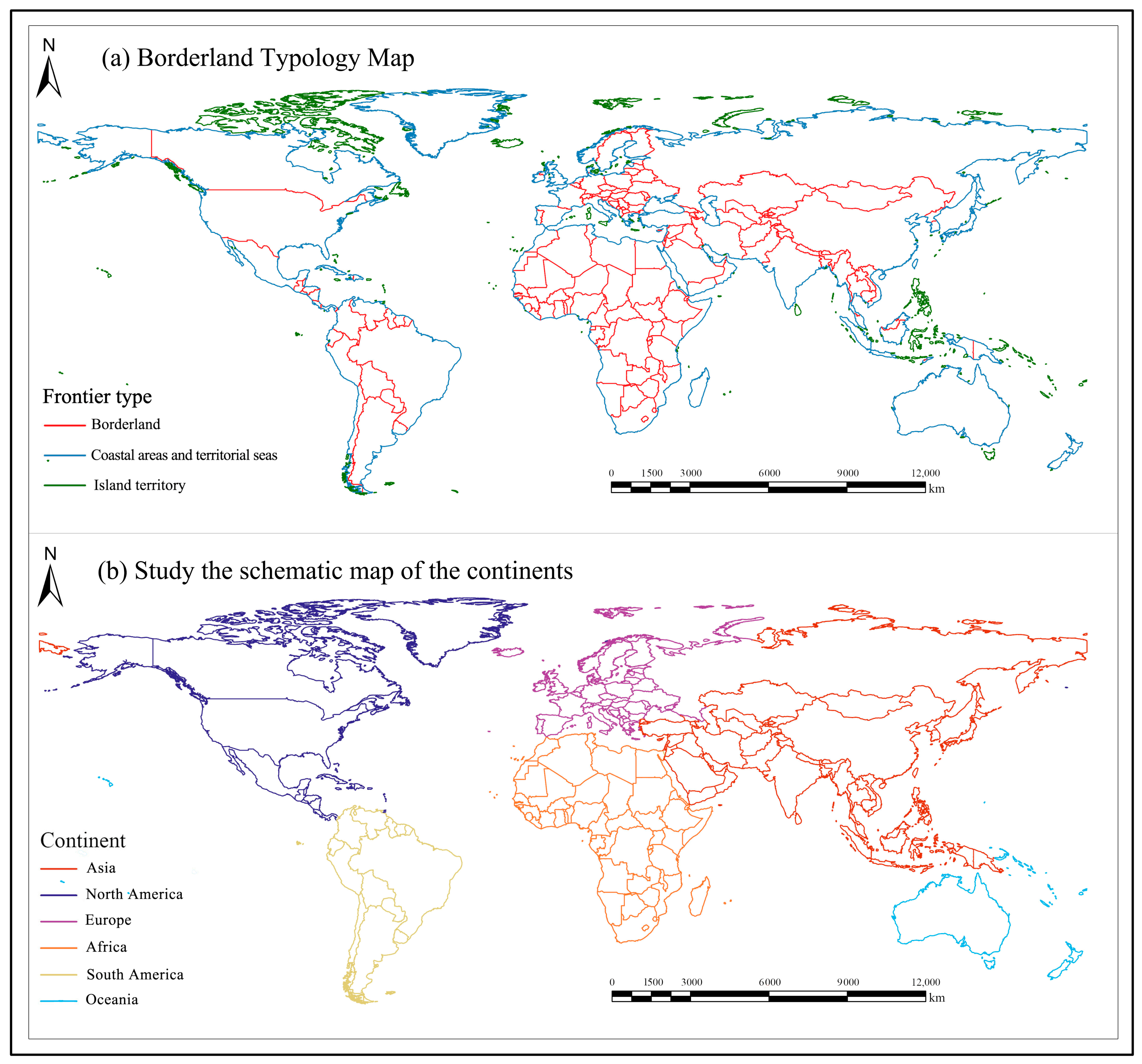
The 150 km buffer represents the wider border–hinterland scale. It captures the potential interaction of border regions with regional urban networks, ecological systems, major agricultural areas, and broader spatial governance contexts. Extending the buffer beyond this distance would substantially increase the inclusion of national interior areas and could weaken the analytical distinction between border-related processes and general national land-use change (Figure 1).

A constant 50 km interval was adopted to maintain a regular nested structure and to allow direct comparison of indicator changes with increasing distance from the boundary. The interval is also substantially larger than the 300 m spatial resolution of the land-cover dataset, thereby reducing the influence of individual-pixel uncertainty on buffer-level estimates. The 50–100–150 km design therefore balances three requirements: sensitivity to localized border change, representation of intermediate corridor processes, and inclusion of broader hinterland interactions.

The selected buffer distances should not be interpreted as fixed or universally applicable thresholds of the border effect. Instead, they are standardized analytical scales used to test whether the magnitude, ranking, and transition structure of land-use change remain stable or change systematically as the spatial window expands.

To ensure analytical consistency and comparability at the global scale, several preprocessing steps are applied. Antarctica is excluded due to its unique governance regime and atypical land use processes. Additionally, small spatial units (<10 km²), such as minor islands and fragmented patches, are removed to reduce geometric noise and area bias during vector processing and buffer construction. These steps ensure stable and consistent spatial units for multi-scale analysis.

Based on spatial topology and geographic characteristics, border segments are further classified into three types: terrestrial borders, coastal borders, and island borders, which are used for subsequent typological analysis.

2.1.2. Land Use Data

Land use data are obtained from the ESA Climate Change Initiative (CCI) Land Cover dataset, with a spatial resolution of 300 m × 300 m. Four benchmark years—1992, 2000, 2010, and 2020—are selected, providing consistent classification standards and strong temporal comparability.

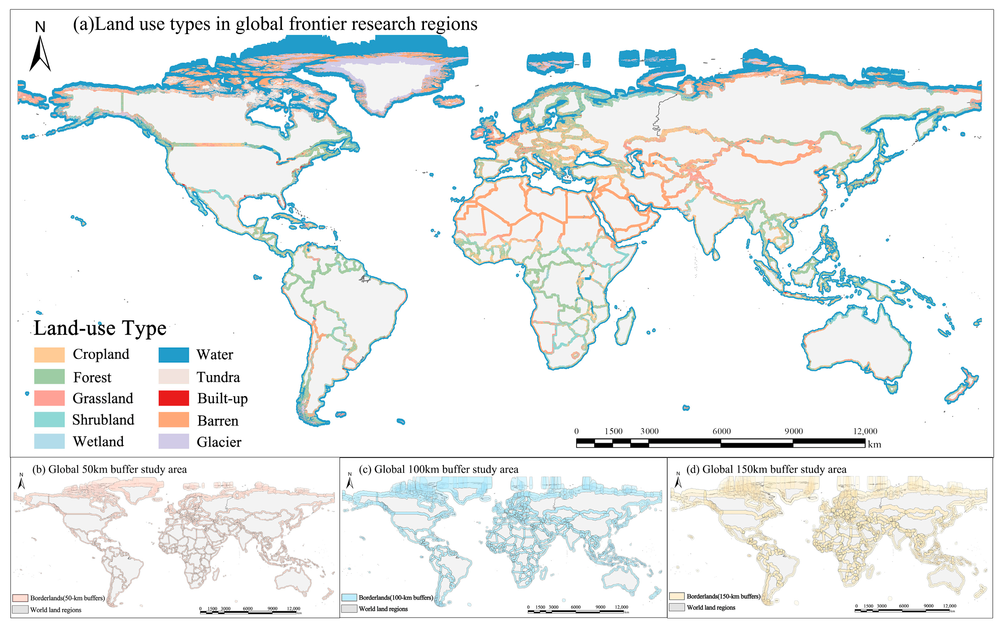
Following the classification scheme of GlobeLand30, the original 22 land cover categories are reclassified into 10 aggregated types: cropland, forest, grassland, shrubland, wetland, water bodies, tundra, artificial surfaces, bare land, and permanent ice and snow. Land use data within each buffer zone are extracted using ArcGIS, and time-series datasets, transition matrices, and dynamic change indicators are constructed to support subsequent analyses (Figure 2).

2.2. Analytical Methods and Indicator Interpretation

2.2.1. Analytical Methods

To systematically characterize land use evolution in border regions, an indicator system is developed across four dimensions: change rate, structural diversity, transition dynamics, and development intensity. The system includes the Single Land Use Dynamic Degree (SLUDD), Integrated Land Use Dynamic Degree (ILUDD), Weighted Composite Transition Intensity (W), and land use spatial differentiation index (ALTR) (

Table 1. Interpretation and calculation logic of the land-use change indicators.

Indicator	Main Analytical Question	Numerator	Denominator	Interpretation	Principal Sensitivity
SLUDD	Is a land class expanding or contracting?	Net area change of class (i)	Initial area of class (i) and period length	Annual net directional change	Small initial class area and gain–loss cancellation
ILUDD	How much of the whole land system was converted?	Total off-diagonal transition area	Initial valid land area and period length	Gross system-wide turnover intensity	Number and aggregation of land classes
W	Which boundary segments have the greatest composite transition activity?	Weighted off-diagonal transition area	Valid land area and period length	Weighted, area-normalized transition intensity	Weighting rule, class imbalance, and marine pixels
ALTR	Which directional transition pathway is dominant?	Area converted from class (i) to class (j)	Initial area of source class (i) and period length	Annual directional substitution rate	Rare source classes and classification confusion

).

(1)

Single Land Use Dynamic Degree (SLUDD)

SLUDD measures the annual rate of expansion or contraction of a specific land use type over a given period. This indicator originates from the land use dynamic degree model proposed by Wang Xiulan and Bao Yuhai and has been widely applied in land use change studies [17]. For example, Xiao [18] also extended this prototype in their optimization model construction. Relevant standards quote the following calculation formula as follows:

$$\mathrm{S}\mathrm{L}\mathrm{U}\mathrm{D}\mathrm{D}={\displaystyle \frac{{LA}_{i,t+1}-{LA}_{i,t}}{{LA}_{i,t}}}\times {\displaystyle \frac{1}{T}}\times 100\%$$

$i$: The number of land use types;

$t$, $t+1$: The beginning year and the end year of the study period, respectively;

${LA}_{i,t}$: The area of the i-th land use type in year t at the beginning of the period;

$T$: Time span.

SLUDD is classified into five levels based on change rates: significant decrease (≤−0.05), slight decrease (−0.05 to −0.01), stable (−0.01 to +0.01), slight increase (+0.01 to +0.05), and significant increase (≥+0.05).

(2)

Integrated Land Use Dynamic Degree (ILUDD)

ILUDD captures the structural complexity of land use change within a region over a given time period. Based on the land use transition matrix, it emphasizes the intensity of inter-type conversions and reflects systemic restructuring processes within the land use system. This indicator comprehensively refers to the transfer diversity measurement method [19] and the logic of ecosystem structure dynamic modeling [20]. In recent years, similar ideas have been widely applied to the dynamic change in land use caused by urbanization and the analysis of ecosystem service value [21], reflecting the important role of structural change in spatial decision-making:

$$\mathrm{I}\mathrm{L}\mathrm{U}\mathrm{D}\mathrm{D}=\left({\displaystyle \frac{{\displaystyle {\sum }_{i=1}^n}{\displaystyle {\sum }_{j=1}^n}∆{LA}_{i,j}}{{\displaystyle {\sum }_{i=1}^n}∆{LA}_{i,t}}}\right)\times {\displaystyle \frac{1}{T}}\times 100\%$$

$n$: Total number of land use types divided by the study area;

$i$: Land use type number at the beginning of the period;

$j$: Land use type number at the end of the period;

$∆{LA}_{i,j}$: The area converted from the i-th land type to the j-th land type corresponds to the elements in the i-th row and j-th column of the land use transfer matrix;

$T$: Time span.

This indicator is particularly suitable for describing the evolution of land use patterns and is classified into five levels: very low (0–0.0005), low (0.0005–0.0015), moderate (0.0015–0.003), high (0.003–0.005), and very high (>0.005).

(3)

Weighted Composite Transition Intensity (W)

The Weighted Composite Transition Intensity (W) measures the overall frequency of land use transitions within a given boundary segment over a specified period. By introducing weights, it reflects the relative importance of different land use types in the transition process.

This indicator is derived from the land use transition matrix and accounts for both total transition volume and type-specific contributions. It is particularly effective for identifying dynamic evolution patterns within boundary buffer zones [22,23].

$$W_b^{*}={\displaystyle \frac{{\displaystyle {\sum }_{i=1}^n}{\sum }_{j\ne i}{\omega }_i\cdot T_{ij}^b}{A_{total}^b\times T}}$$

$W_b^{*}$: weighted comprehensive transfer frequency of boundary b;

${\omega }_i$: weight of land type i (no weight if set to 1);

$T_{ij}^b$: the transfer area from type i to type j in boundary b;

$A_{total}^b$: the total area of the buffer corresponding to boundary b;

$T$: time span.

Based on the distribution of empirical data, W is classified into five levels using a quantile-based approach, namely extremely low, low, moderate, high, and extremely high transition zones, ensuring comparability across different buffer scales.

(4)

Land Use Spatial Differentiation Index (ALTR)

ALTR measures the annual rate at which one land use type is structurally converted into another, normalized by the initial land area [24]. It emphasizes directional substitution processes and is suitable for analyzing spatial restructuring and land use transitions in border regions [25].

$$\mathrm{A}\mathrm{L}\mathrm{T}\mathrm{R}={\displaystyle \frac{\left|{LA}_A\right.\left.\to {LA}_B\right|}{{LA}_{A,t}}}\times {\displaystyle \frac{1}{T}}\times 100\%$$

${LA}_{A,t}$: Total area of land type a transferred out at time t at the beginning of the period;

LA_A→B: Area converted from land use type A to land use type B;

$T$: Time span.

The index is classified into five levels, ranging from very low to extremely high differentiation. Higher ALTR values indicate stronger spatial heterogeneity and more pronounced structural differentiation within border regions.

(5)

Multiple linear regression analysis of land use change (LUCR)

In order to further test the relationship between land use change and socio-economic factors at the border, this paper takes a 50 km buffer zone as the analysis scale and the buffer zone unit corresponding to each boundary as the basic sample, and constructs the regression model of driving factors of land use change from 2000 to 2020. The dependent variable is the proportion of land use change (lucr_0020), that is, the proportion of land use type change in the buffer zone in the total effective land use area from 2000 to 2020. The explanatory variables include population density change (pop_chg), GDP change (gdp_chg) and night light change (ntl_chg), which respectively represent the changes in population agglomeration, economic development and human activity intensity.

In terms of model setting, this paper first constructs a basic model, which only includes three explanatory variables, population, GDP and luminous intensity; then, frontier type control variables and continent control variables are added to test the impact of different spatial types and regional backgrounds on land use change. Frontier types include land, sea and island, with land as the reference group; Asia was used as the reference group for continent control variables. The model form is as follows:

$${\mathrm{L}\mathrm{U}\mathrm{C}\mathrm{R}}_{2000–2020}={\beta }_0+{\beta }_1\ln \left(pop\_chg\right)+{\beta }_2\ln \left(gdp\_chg\right)+{\beta }_3\ln \left(ntl\_chg\right)+ϵ$$

${\beta }_0$: Regression constant term (intercept);

${\beta }_1\ln \left(pop\_chg\right)$: POP_chg = ln(pop_2020 + 1) − ln(pop_2000 + 1);

${\beta }_2\ln \left(gdp\_chg\right)$: GDP_chg = ln(gdp_2020 + 1) − ln(gdp_2000 + 1);

${\beta }_3\ln \left(ntl\_chg\right)$: NTL_chg = ln(ntl_2020 + 1) − ln(ntl_2000 + 1);

$ϵ$: Random disturbance term (residual).

Considering the limited availability of nighttime lighting data around 2000, this paper takes the nighttime lighting in 2004 as an approximate representation of human activity intensity around 2000.Among them, ntl_2000 is approximately characterized by the night light data in 2004. Logarithmic variation can reduce the influence of dimensional difference and extreme value of different variables on model estimation.

2.2.2. Indicator Interpretation

Classification was used only for cartographic visualization. To ensure cross-scale comparability, thresholds were derived from the pooled sample containing all boundary segments, periods, and buffer distances. ILUDD and ALTR were classified using pooled quintiles, whereas the strongly right-skewed W distribution was classified using P50, P75, P90, and P95 to retain information on high-intensity tails. All statistical tests and model estimations used the original continuous indicator values.

2.2.3. Sensitivity and Robustness Analysis

Indicator sensitivity was evaluated in relation to spatial scale, land-cover classification structure, weighting specification, and coastal data treatment. First, Spearman rank correlations and top-decile hotspot overlap were calculated among the 50, 100, and 150 km buffers. Second, ILUDD and W were recalculated using alternative land-cover aggregation schemes to examine sensitivity to the number and composition of land classes. Third, the weighted and equal-weight versions of W were compared. Fourth, coastal and island indicators were recalculated after masking permanent marine pixels and resolving overlapping buffer geometries.

An indicator was considered structurally robust when cross-scale or cross-specification rank correlations exceeded the predefined criterion, relative deviations remained limited, and the main hotspot boundaries and dominant transition pathways were preserved. These tests distinguish substantive border-land dynamics from changes caused by analytical scale or data structure.

2.3. Research Framework

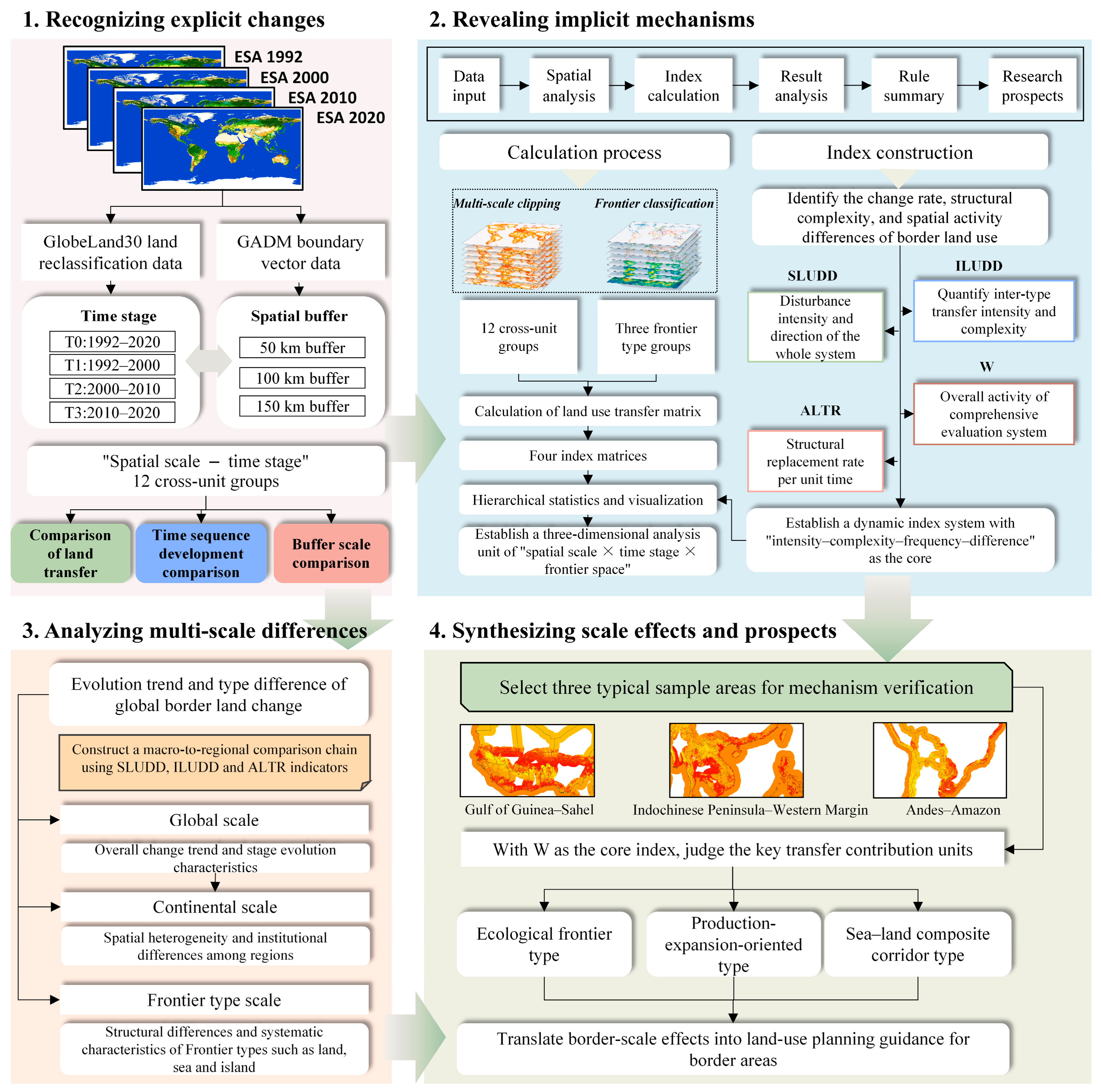
This study establishes a four-dimensional analytical framework integrating spatial scale, temporal stage, border type, and scale analysis. Based on land use data from 1992 to 2020, three buffer zones and three evolutionary stages are defined, along with three border types (terrestrial, coastal, and island), forming a unified classification structure (Figure 3).

Within this framework, the indicator system is used to identify change rates, structural transformations, and intensity dynamics of land systems, enabling classification and stage-specific characterization of border land use patterns and providing technical support for subsequent spatial differentiation analysis.

3. Results

3.1. Differences Across Border Types

Border land use dynamics exhibit clear typological divergence, with terrestrial, coastal, and island borders following fundamentally distinct evolutionary trajectories in terms of intensity, structural complexity, and transition regimes (Figure 4).

In terms of change intensity, all border types share a common trend of built-up land expansion; however, they differ significantly in rates, temporal peaks, and associated changes in cropland and forest. Terrestrial borders experienced the most pronounced urban expansion during 2000–2010, with the annual growth rate of built-up land exceeding 5% within the 50 km buffer—substantially higher than that of coastal (3.8%) and island borders (2.6%). Cropland dynamics diverge notably: coastal borders showed an early net decline in the 2000s (approximately −0.03% annually), terrestrial borders maintained slight growth during the same period, and island borders experienced a marked reduction (−0.26% annually). Forest dynamics further highlight differentiation: terrestrial borders shifted to net growth after 2010, island borders entered a recovery phase earlier (2000s), whereas coastal borders continued to decline, albeit at a decreasing rate.

These patterns indicate that terrestrial and island borders are characterized by multi-directional transitions combining development and ecological recovery, whereas coastal borders are dominated by a unidirectional urbanization-driven transformation.

From the perspective of structural complexity, land use transitions differ markedly among border types. Coastal borders exhibit relatively simple and linear transformation pathways, while terrestrial borders display more diversified transitions involving both development (e.g., conversion of unused land to cropland or grassland) and ecological processes (e.g., forest recovery and water body shrinkage). Island borders show the highest complexity, as reflected by ILUDD values, due to the simultaneous occurrence of multiple large-scale transitions. During 2000–2010, island regions underwent coordinated processes including cropland contraction, forest expansion, grassland stabilization, and continuous growth of built-up land—indicating a dual transition from agricultural land toward both ecological and urban land uses.

The high structural complexity of island borders suggests strong sensitivity to coupled human–environment interactions, making them key zones for observing rapid systemic reconfiguration.

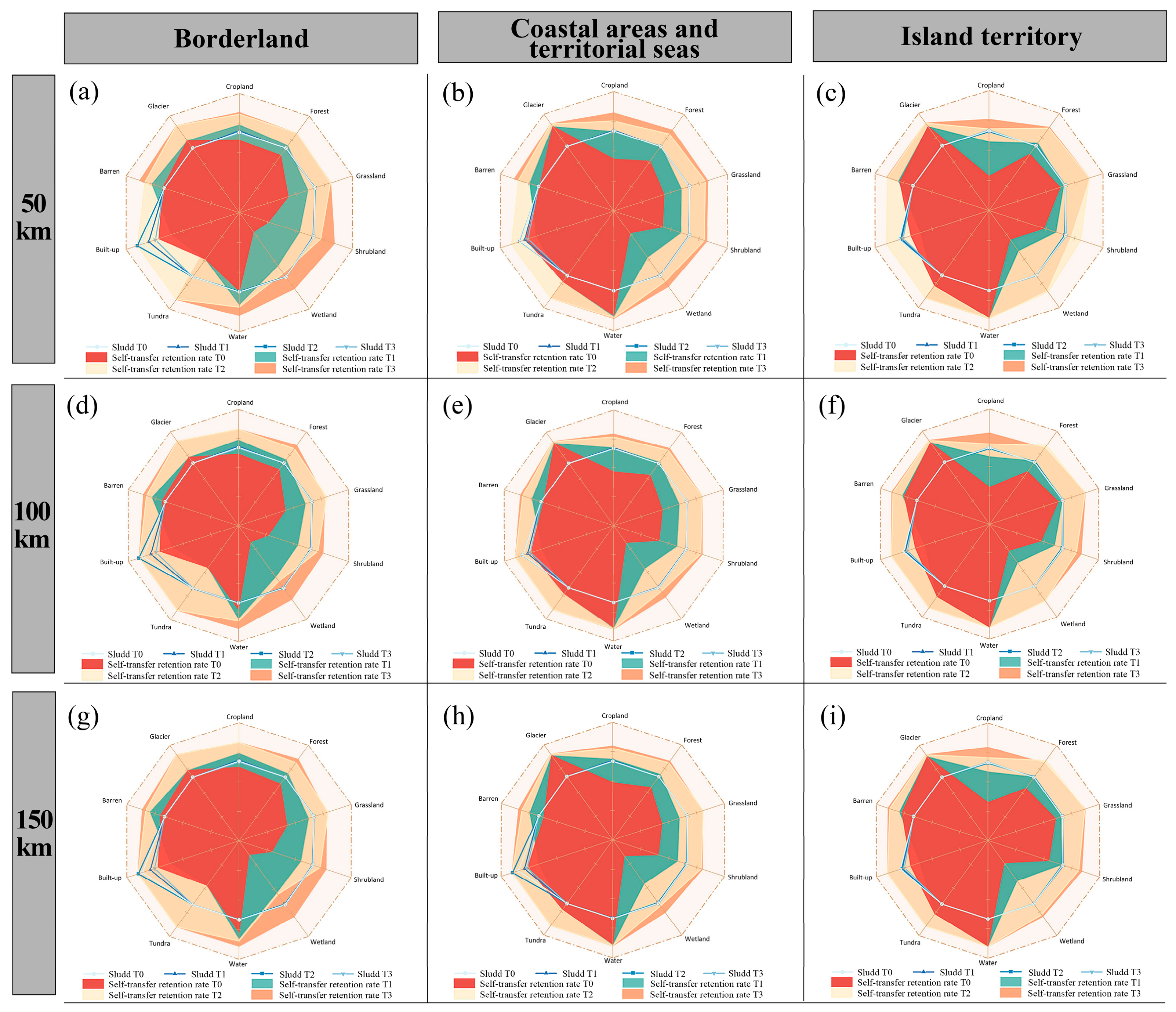
In terms of transition frequency and stability, the weighted transition frequency (W) reveals significant differences in land system stability. Cropland retention rates are lowest in island borders (88%), compared to terrestrial (94%) and coastal (91%) borders, with major transitions directed toward forest and built-up land. Coastal borders are characterized by large-scale conversion of cropland to built-up land, reflecting coastal urbanization processes. Built-up land exhibits near-complete retention (~100%) across all border types, indicating strong irreversibility. In terrestrial borders, water bodies show relatively low retention (<87%), and unused land continues to decline, reflecting the combined effects of agricultural expansion and environmental change (Figure 5).

Overall, transition frequency patterns highlight the asymmetric stability of land types, with built-up land acting as a terminal state in land system evolution.

From a temporal perspective, border land use evolution follows a three-stage trajectory:

• T1 (1992–2000): Initial adjustment phase, characterized by moderate changes. Terrestrial borders were dominated by conversion of unused land to cropland and grassland; coastal borders showed early signs of development; island borders were in an exploratory stage of land allocation.
• T2 (2000–2010): Rapid transformation phase, marked by intensive expansion of built-up land across all border types. Cropland declined sharply in coastal and island borders, while terrestrial cropland stabilized. Simultaneously, forest and grassland areas increased, indicating the combined influence of urbanization and ecological restoration.
• T3 (2010–2020): Stabilization phase, during which urban expansion slowed significantly, cropland loss was mitigated, and forest areas continued to grow modestly. Land systems entered a “development–conservation balance” regime.

This staged evolution reflects a global shift from extensive land transformation toward more regulated and adaptive land system management.

To facilitate a direct comparison among the three border types, the principal characteristics identified from the land-use dynamic indicators and transition matrices are summarized in

Table 2. Comparative characteristics of land-use change among terrestrial, coastal, and island borders from 1992 to 2020.

Comparative Dimension	Terrestrial Borders	Coastal Borders	Island Borders
Principal spatial context	Interfaces between neighboring sovereign territories, strongly affected by institutional differences, cross-border accessibility, and inland transport corridors	Land–sea interfaces influenced by coastal urbanization, port development, population concentration, and shoreline constraints	Spatially confined land systems with high exposure to land–sea interactions and limited land availability
Built-up land dynamics	Strongest expansion during 2000–2010; the annual growth rate exceeded 5% within the 50 km buffer	Continuous expansion, with an annual growth rate of approximately 3.8% during 2000–2010 within the 50 km buffer	Persistent but comparatively lower expansion, with an annual growth rate of approximately 2.6% during 2000–2010 within the 50 km buffer
Cropland dynamics	Generally stable or slightly increasing during the rapid transformation stage	Net contraction, closely associated with conversion to built-up land	Most pronounced contraction; the annual decline reached approximately 0.26% during 2000–2010
Forest dynamics	Shifted from loss or fluctuation to net recovery after 2010	Continued to decline, although the rate of decline gradually decreased	Entered a recovery phase earlier than the other types, particularly after 2000
Dominant transition pathways	Multiple pathways involving unused land–cropland, unused land–grassland, cropland–built-up land, and cropland–forest transitions	Relatively concentrated conversion from cropland to built-up land	Concurrent cropland-to-forest, cropland-to-built-up land, and vegetation restructuring
Transition structure	Diversified and bidirectional, combining development expansion and ecological restoration	Relatively simple and directional, dominated by urbanization-related substitution	Highest degree of simultaneous multi-type transition and systemic restructuring
Cropland retention rate	Approximately 94%, indicating comparatively high agricultural stability	Approximately 91%, with evident development-related conversion pressure	Approximately 88%, indicating the lowest cropland stability among the three types
Overall evolutionary mode	Development–restoration composite transition	Urbanization-dominated directional transition	Agricultural contraction–ecological recovery–built-up expansion composite transition
Main interpretive implication	Land-use change reflects the interaction of boundary institutions, development corridors, agricultural use, and ecological restoration	Land-use change is strongly associated with concentrated coastal development and competition for limited coastal land	Land-use change reflects high sensitivity to land scarcity, environmental change, and coupled human–environment pressures

Note: The built-up land growth rates and cropland decline rates reported in the table refer to the 2000–2010 period within the 50 km buffer. The retention rates represent the comparative results reported for the three border types. The table summarizes the dominant tendencies and does not imply that all individual boundary segments follow the same trajectory.

. Although built-up expansion occurred in all three types, the associated land conversion pathways, ecological responses, and system stability differed substantially. Terrestrial borders were characterized by diversified and stage-dependent transitions, coastal borders exhibited a relatively concentrated urbanization pathway, and island borders experienced the strongest simultaneous restructuring of agricultural, ecological, and built-up land.

Table 3. Statistical table of comprehensive transfer intensity of border land at various scales.

Buffer (km)	Average	Median	Total	Zero-Value Boundary (Strip)
50	0.00485	0.00413	2.349	13
100	0.00434	0.00384	2.040	17
150	0.00402	0.00344	1.834	25

reveals that the typological differences are not limited to variations in change magnitude. More importantly, the three border types differ in the organization of their transition pathways. Terrestrial borders contain a wider combination of production expansion, urban development, and ecological restoration. Coastal borders are more strongly characterized by concentrated substitution from cropland to built-up land. Island borders show the lowest cropland stability and the most pronounced concurrence of agricultural contraction, forest recovery, and built-up expansion. These differences demonstrate that border type affects not only the intensity of land-use change but also the structural direction and stability of land-system transformation.

3.2. Global-Scale Characteristics

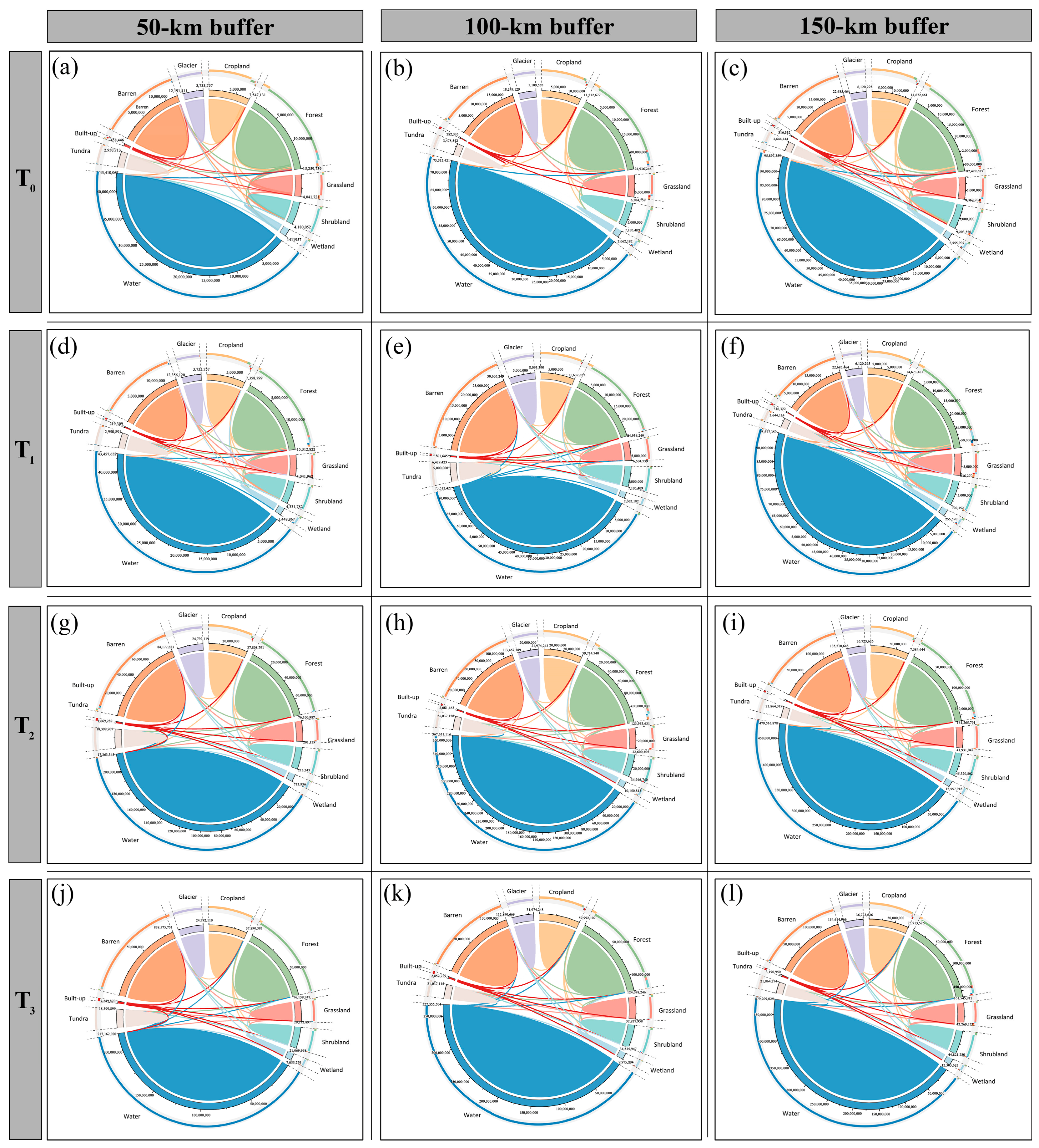
At the global scale, border land use systems have undergone a clear transition from high-intensity instability in the 1990s to increasing stability after 2000, accompanied by persistent directional transformations among key land types (Figure 6).

In terms of system stability, most land use types exhibit retention rates exceeding 90% throughout the study period, with stability increasing over time. Built-up land and water bodies are the most stable categories, with built-up land showing virtually no reverse conversion after 2000. Wetlands, although initially the least stable, demonstrate the most significant improvement in retention rates.

Spatially, stability varies across buffer zones. The 50 km near-boundary zone shows relatively lower retention due to direct urban expansion pressures, whereas the 100–150 km zones reflect broader ecological and agricultural processes. Among land types, wetlands remain the most volatile, followed by grassland and shrubland, while cropland and forest maintain relatively high and stable retention rates.

These findings suggest that border proximity amplifies land system sensitivity, while broader regional contexts promote stabilization.

In terms of transition pathways, global border land use change exhibits clear directional and stage-dependent characteristics. Cropland-to-forest conversion emerges as a dominant and persistent process, accounting for approximately 5–6% of total cropland over the study period, with acceleration after 2000. This trend reflects large-scale ecological restoration efforts and contributes to improved ecosystem stability and services.

Simultaneously, cropland-to-built-up conversion represents another major pathway, peaking during 2000–2010 (~0.97%), corresponding to the global urbanization surge. Additional transitions include widespread conversion of grassland and shrubland to forest, contributing to increased forest coverage, and complex wetland transitions toward both forest and water bodies, indicating high environmental sensitivity.

These directional transitions reveal a dual process of ecological restoration and urban expansion shaping global border land systems.

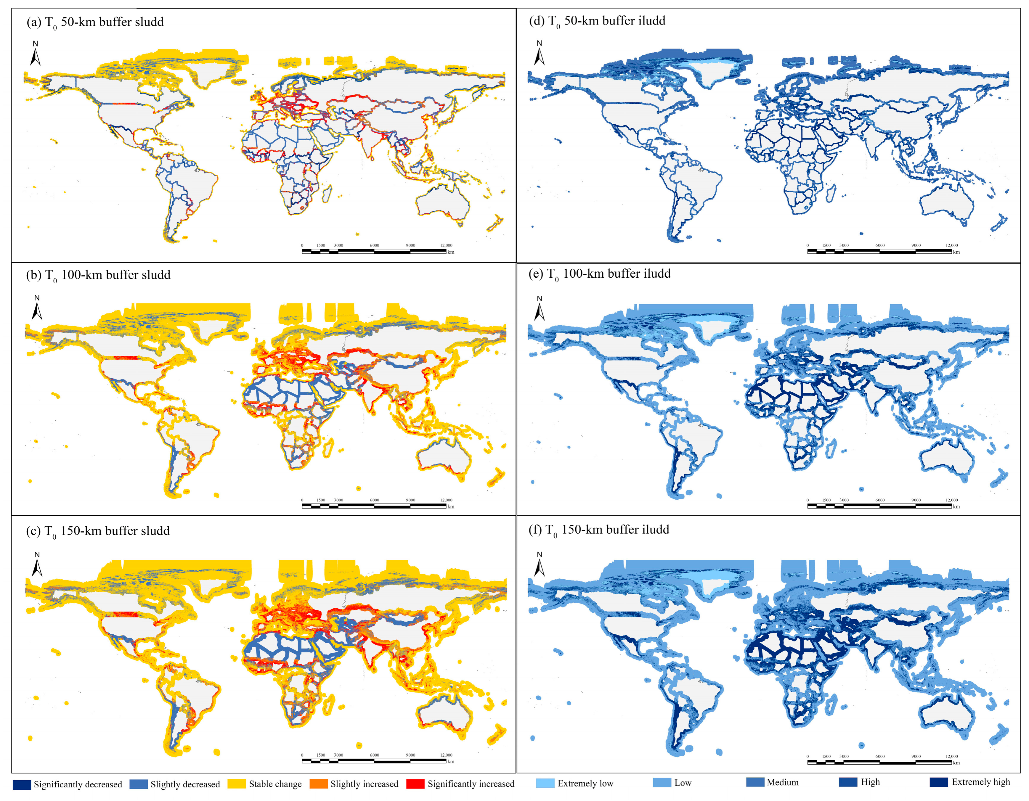
Multi-scale analysis further reveals strong scale effects and gradient patterns. The 50 km buffer exhibits high volatility in early stages followed by stabilization, with changes concentrated in fragmented and localized patterns. The 100 km buffer maintains relatively stable, low-intensity dynamics throughout, reflecting policy-regulated regional systems. The 150 km buffer shows intermediate intensity initially, later stabilizing, with mixed processes of urban expansion and ecological restoration (Figure 7).

This gradient structure indicates that boundary effects are strongest at close range and progressively attenuate with distance, while regional processes become increasingly dominant.

Joint analysis of SLUDD and ILUDD highlights distinct spatial regimes:

• Contraction zones (SLUDD ≤ −0.05) are concentrated in North Africa, South Asia, and parts of South America, reflecting combined pressures of ecological degradation and agricultural marginalization.
• Expansion zones (SLUDD ≥ 0.05) are located in East Asia, Europe, and eastern North America, driven by urbanization and industrial expansion.
• Transition zones dominate most border regions, characterized by gradual and incremental land transformations.

ILUDD patterns further reveal multi-scale response mechanisms. High-value clusters are scattered within the 50 km buffer (e.g., Great Lakes region, Mongolia–Russia border), reflecting localized boundary effects. At broader scales, these clusters evolve into corridor-like or aggregated patterns, indicating increasing dominance of regional drivers.

Importantly, high ILUDD values reflect structural instability rather than simply urbanization intensity, highlighting the role of multi-type interactions in shaping land systems.

3.3. Continental-Scale Differentiation

At the continental scale, border land use change forms a stable yet differentiated regime characterized by systematic variations in intensity, spatial gradients, and transition structures, reflecting the combined effects of development stage, institutional openness, and ecological constraints.

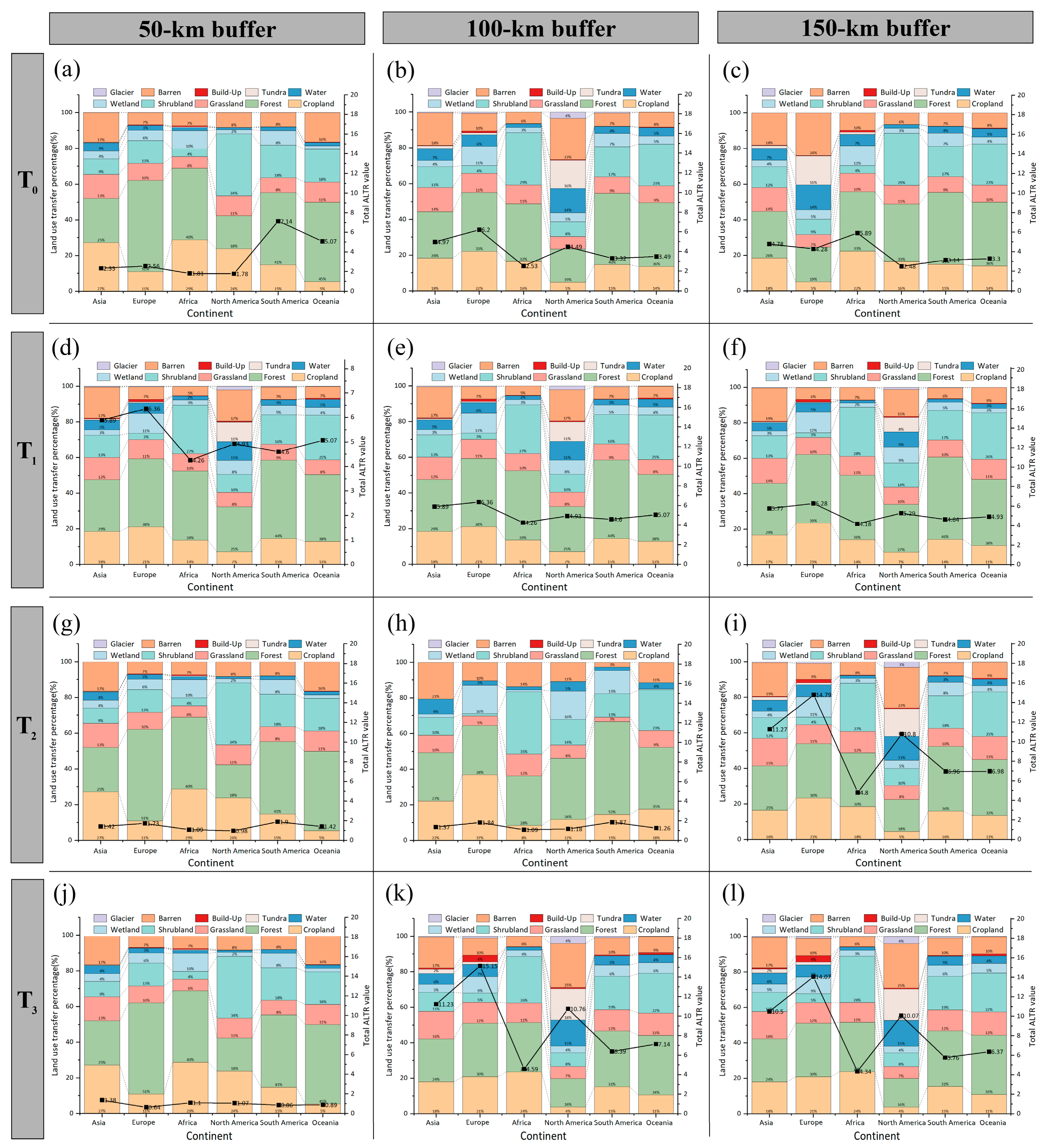
From a temporal perspective, all continents exhibit a broadly consistent three-phase trajectory, albeit with differing magnitudes. The 1990s represent a high-intensity restructuring phase, during which Africa, Oceania, and South America show the highest levels of land use substitution, while Asia, Europe, and North America remain at moderate levels. During 2000–2010, most continents enter a plateau phase, with reduced transition intensity. After 2010, border land systems become re-activated, though in a more regulated manner. Over the long term, a clear pattern emerges: Oceania exhibits the highest overall transition intensity, whereas Asia remains relatively stable, forming a contrast between highly dynamic “island–coastal systems” and comparatively stable “terrestrial border systems” (Figure 8).

This temporal divergence indicates that global border land systems are not synchronized but instead reflect region-specific development trajectories and policy cycles.

From a spatial gradient perspective, buffer zones reveal distinct patterns of scale-dependent differentiation. During 1992–2010, the 100 km buffer generally exhibits higher transition intensity than the 50 km and 150 km buffers, suggesting the dominance of regional-scale processes. However, during 2010–2020, this pattern reverses, with the 50 km near-boundary zone showing accelerated adjustment—indicating a shift toward boundary-proximate intensification. This “near-field intensification and far-field attenuation” pattern is most pronounced in Africa and South America, while Asia and Europe display relatively smoother gradients.

These findings suggest a reconfiguration of spatial drivers, with boundary effects becoming more localized in recent decades.

From a structural perspective, continents differ significantly in dominant transition pathways and the concentration of land use types. Asia is characterized by reciprocal transformations between forest and cropland, reflecting a balance between agricultural production and ecological restoration. Africa exhibits a cyclic transition structure centered on forest land, indicating repeated conversions among forest, grassland, and cropland under ecological and demographic pressures. Oceania is dominated by reversible transitions between forest and shrubland, suggesting a relatively flexible ecological adjustment system.

In contrast, Europe and North America are primarily driven by the conversion of agricultural land to built-up areas, reflecting mature urbanization processes and spatial restructuring. South America is distinguished by large-scale conversion of forest to agricultural land, indicating the expansion of agricultural frontiers.

Moreover, transition structures in Africa and Oceania are more concentrated, whereas North America displays higher structural complexity and diversification.

Taken together, these patterns form a three-dimensional differentiation framework of “intensity–gradient–structure”, within which:

• Oceania represents a dynamic equilibrium system balancing ecological processes and development;
• Africa exhibits extensive and high-intensity substitution across large spatial extents;
• South America reflects coupled ecological–policy boundary effects, particularly in forest frontiers;
• Europe and North America demonstrate institution-driven regeneration and urban restructuring;
• Asia shows low-intensity but bidirectional and complex transitions.

These intercontinental differences can be interpreted as the outcome of interacting institutional, economic, and environmental drivers, with scale effects further modulating their spatial expression.

Importantly, natural and productive land types—such as forest, cropland, and grassland—constitute the structural backbone of land transitions, whereas urban expansion, although significant, is not the sole dominant driver. Wetlands and water bodies exhibit strong regional specificity and serve as sensitive indicators of environmental change.

The observed scale sensitivity further indicates that 50 km buffers capture node- and corridor-level disturbances, while 100–150 km buffers better represent systemic regional dynamics.

3.4. Key Regions and Representative Patterns

3.4.1. Analysis of Land Use Transfer

Global border land use change is highly uneven and concentrated, with a small proportion of boundary segments accounting for a disproportionate share of total transition intensity, reflecting strong spatial clustering and “hotspot” dynamics (Table 3).

Across the three buffer scales, the weighted transition intensity (W) consistently declines with increasing buffer distance. The mean W decreases from 0.00485 (50 km) to 0.00402 (150 km), while the number of inactive (zero-change) boundary segments increases. However, this attenuation does not imply homogenization. Instead, larger buffers incorporate more stable hinterland areas, diluting overall intensity while simultaneously amplifying relative differences among active boundary segments.

Crucially, the relative ranking of boundary activity remains highly consistent across scales (correlation coefficients: 0.812–0.932), indicating that spatial patterns of land use dynamics are structurally robust. The top 10% most active boundary segments consistently contribute approximately 26–27% of total transition intensity, confirming that global border change is highly concentrated rather than uniformly distributed.

Different spatial scales correspond to distinct analytical perspectives. The 50 km scale captures high-frequency, near-boundary processes driven by institutional differences and restricted factor flows. The 150 km scale integrates border dynamics with hinterland systems, revealing broader interactions with urban networks, industrial, and ecological contexts.

Notably, not all boundary segments follow a simple distance-decay pattern. Approximately one-third exhibit inverse scale effects, where transition intensity increases with buffer size. For example, inland development corridors (e.g., resource extraction or transport-driven expansion) can amplify land use change in hinterland areas, whereas highly urbanized borders show strong near-boundary concentration that becomes diluted at larger scales.

These findings highlight the coexistence of boundary-driven and hinterland-driven processes, complicating simplistic interpretations of border effects.

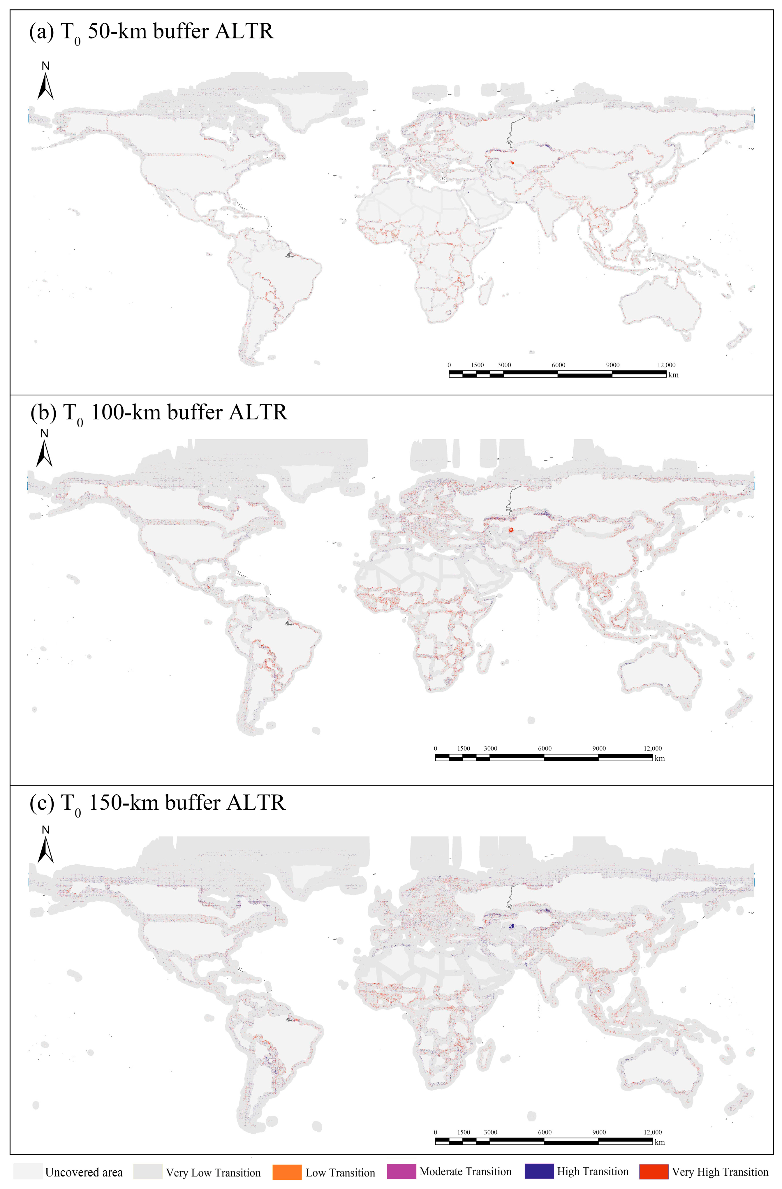
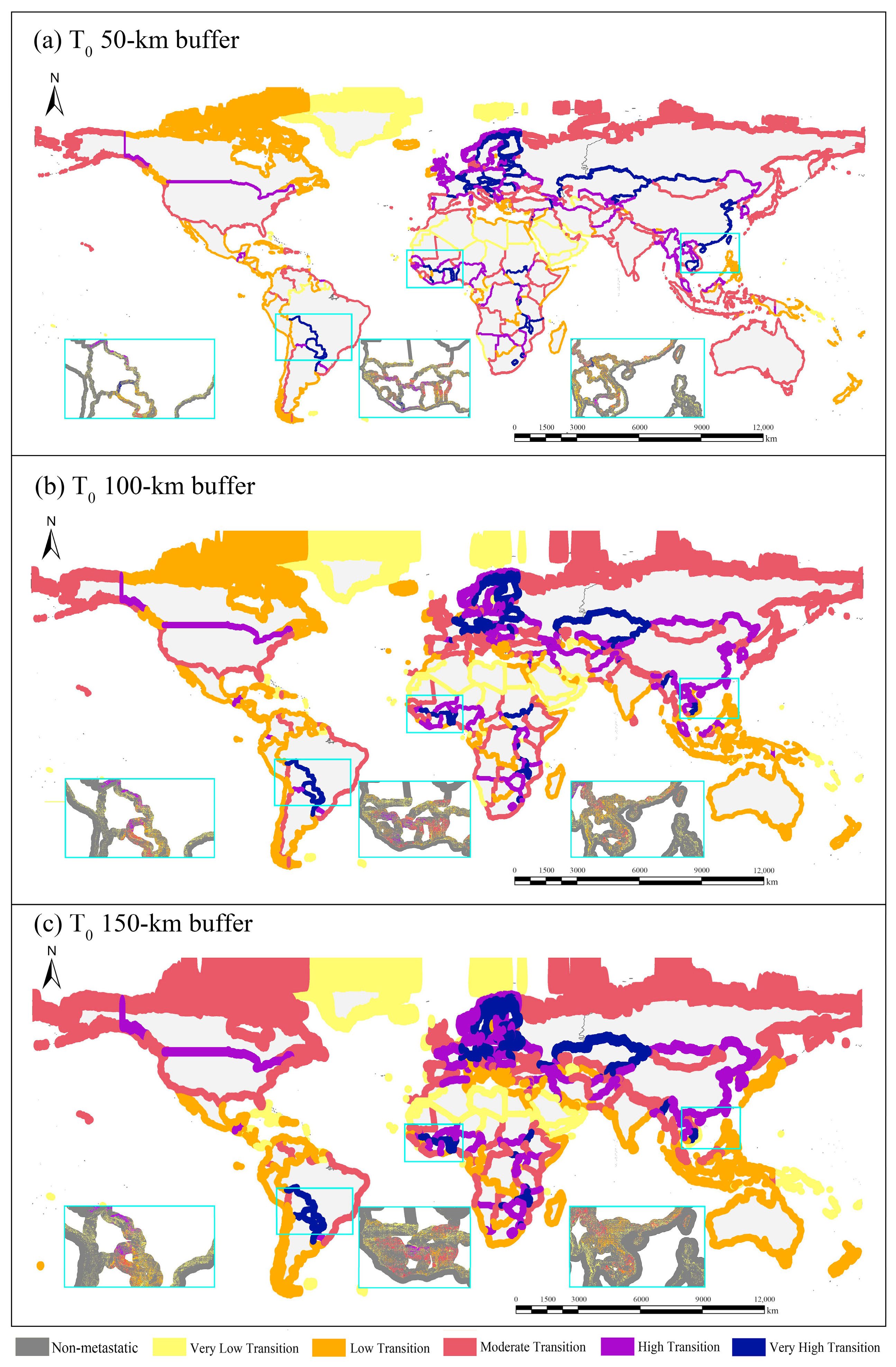
To further elucidate dominant mechanisms, three representative border regions are identified, corresponding to three archetypal evolutionary patterns (Figure 9):

(1)

Forest Frontier Type (Andes–Amazon Transition Zone)

This type is characterized by low overall intensity but localized high-intensity hotspots, reflecting threshold-driven expansion at ecological frontiers.

The dominant transitions involve conversion of forest and shrubland to cropland, accompanied by cyclical interconversion between vegetation types. This pattern reflects the interaction between agricultural expansion and secondary vegetation regeneration. Spatial heterogeneity in accessibility, topography, and resource distribution amplifies boundary effects, leading to localized intensification.

(2)

Agricultural Expansion Type (West Africa: Gulf of Guinea–Sahel Zone)

This type represents the most extensive and continuous high-intensity transition system globally, driven by demographic pressure and land competition.

Transitions are dominated by conversion of grassland and shrubland to cropland, alongside structural reorganization among vegetation types. Unlike localized hotspots, this pattern reflects region-wide systemic transformation, where ecological fragility and development pressure interact to produce sustained high-intensity change.

(3)

Land–Sea Composite Corridor Type (Mainland Southeast Asia–South China Sea Margin)

This type exhibits strong near-boundary clustering of high-intensity change, reflecting corridor-based development and coastal–border interactions.

Land transitions include forest-to-cropland conversion, urban expansion, and fluctuations in wetlands and water bodies. The spatial pattern is typically “bead-like” along transport corridors and coastal zones, with intensity declining sharply as buffer distance increases.

This highlights the organizing role of infrastructure, ports, and coastal economies in shaping land use patterns within narrow border corridors.

Across all scales, core transition pathways remain remarkably consistent, indicating stable global drivers of land system reorganization. Forest-to-cropland conversion remains the dominant process (15.55–16.84%), followed by cropland-to-built-up conversion (6.31–7.46%). Meanwhile, forest–shrubland interconversion increases with scale, reflecting widespread vegetation restructuring.

From a net change perspective, cropland and built-up land show significant increases, whereas bare land, forest, and shrubland decline overall. This confirms that border regions are not static peripheries but active zones of continuous intensification and restructuring, shaped by both development pressures and ecological processes.

Across the three spatial scales, strong consistency is observed in core transition directions, net change trajectories, and the relative configuration of boundary activity, whereas differences are primarily manifested through scale-induced dilution effects. As the spatial window expands, the average transition intensity declines, high-intensity boundary segments decrease, and low-intensity segments become more prevalent. Meanwhile, the relative ranking of boundary activity is only moderately reshaped within a broader regional context.

These results imply that scale does not fundamentally alter the underlying processes of border land system evolution but instead modulates their observable intensity and spatial expression.

Based on these findings, each analytical scale demonstrates a distinct and complementary applicability. The 50 km buffer is most suitable for capturing direct boundary effects, such as rapid land transformations driven by port development and cross-border regulation. The 100 km buffer balances the preservation of boundary signals with the suppression of extreme-value interference, making it particularly appropriate for cross-regional comparison. The 150 km buffer, by contrast, is better suited for analyzing long-term coupling mechanisms between border zones and their hinterlands, integrating regional development dynamics, ecological transition processes, and boundary effects within a unified analytical framework.

Therefore, the combined use of multi-scale buffers enables a reverse inference of the effective spatial range of boundary effects, providing a methodological basis for matching appropriate observational scales to specific research questions.

In key regions, border land use evolution is characterized by an overall convergence in intensity, a continuous downward shift in structural hierarchy, and persistent “tail resilience” in hotspot boundaries. This internal structure can be effectively revealed using a quantile-based classification of W, which enables precise identification of contribution patterns, as well as temporal and regional differentiation, thereby providing targeted insights for border governance.

Given that W values within individual boundary segments are generally small and highly unevenly distributed—where most units contribute minimally and only a few dominate—direct application of overall intensity classification would compress internal variation and obscure critical contributing units. To address this, a quantile-based five-tier classification scheme is adopted. By integrating all samples from 1992–2020 and using P50, P75, P90, and P95 as thresholds, a standardized contribution hierarchy is constructed.

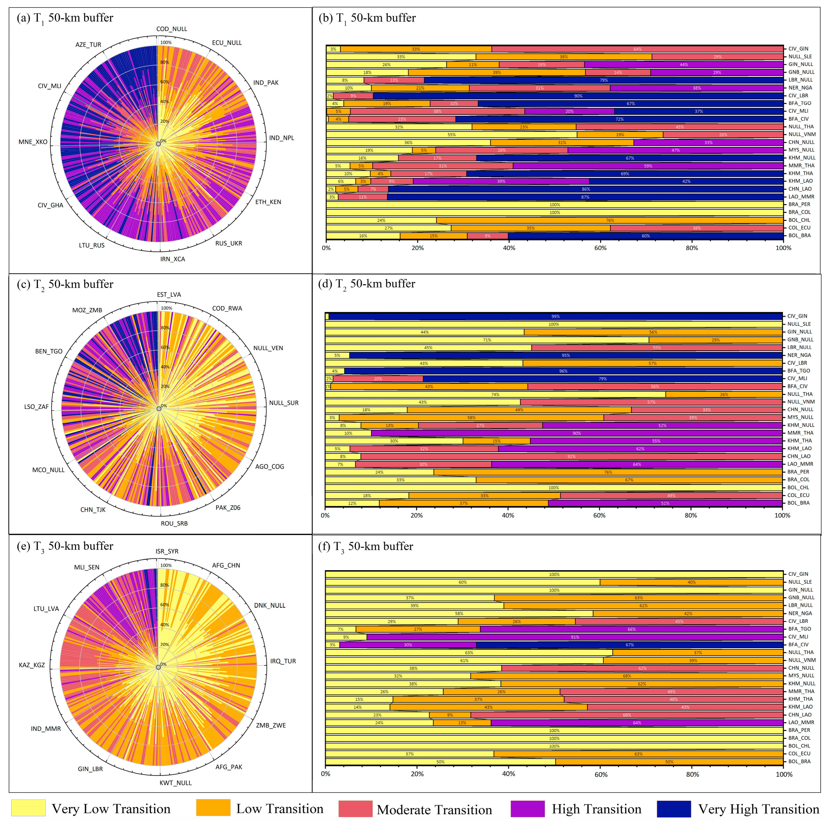
This approach not only accommodates the skewed distribution of the data and ensures balanced sample sizes across classes, but also establishes a consistent basis for cross-temporal and cross-regional comparison of boundary contribution structures(Figure 10).

Temporal dynamics within the 50 km near-boundary zone clearly demonstrate a transition from high-intensity disturbance to stabilized adjustment in border land systems. The mean weighted transition intensity declines steadily from 0.01023 (1992–2000) to 0.00248 (2010–2020), while the number of inactive boundary segments increases from 2 to 15. This shift indicates that land use change is no longer ubiquitously active across all borders but increasingly concentrated in a limited number of key segments and corridor nodes.

Simultaneously, the internal contribution structure undergoes a systematic transformation. The proportion of low-intensity contribution zones rises sharply from 37.91% to 74.70%, whereas the share of extremely high-intensity zones drops dramatically from 30.23% to 2.68%. During the 1990s, land use change was dominated by a small number of extreme-intensity units; after 2010, it transitions toward a regime characterized by moderate-intensity turnover. Moreover, the proportion of boundary segments dominated by a single intensity level continues to increase.

These changes signify a fundamental shift from large-scale structural reorganization to incremental, governance-absorbable adjustments in border land systems. The 25 boundary segments across the three representative regions exhibit markedly divergent evolutionary trajectories, reinforcing the existence of region-specific mechanisms.

• In Southeast Asia, early-stage disturbances are the most intense, with a mean transition intensity of 0.01560 during 1992–2000. Boundary segments such as Laos–Myanmar and China–Laos are dominated by high-intensity structural substitution. However, after 2000, extremely high-intensity contributions decline to zero, and land use dynamics shift toward more moderate adjustments aligned with transportation corridors and industrial belts.
• In West Africa, a strong “hotspot resilience” effect is evident. Despite an overall decline in intensity, extremely high-intensity contributions remain as high as 36.81% during 2000–2010. Boundary segments such as Côte d’Ivoire–Mali continue to exhibit significant fluctuations in later stages, indicating persistent instability and the need for targeted risk management at critical segments.
• In South America, overall intensity remains consistently low, with all transitions shifting to low-intensity adjustments during 2010–2020. Boundary segments such as Brazil–Colombia and Brazil–Peru exhibit minimal change, reflecting a relatively stable land system.

Together, these differentiated trajectories confirm a global transition from widespread abrupt transformations toward corridor- and node-dominated incremental adjustment processes, in which a limited number of high-contribution boundary segments emerge as priority targets for spatial governance.

3.4.2. Drivers of Land-Use Change in Border Regions

Land-use change in border regions results from the combined effects of environmental conditions, ecological processes, and socioeconomic development. The transition analysis reveals a dual trajectory in which built-up expansion, agricultural restructuring, and vegetation recovery occurred simultaneously. This pattern indicates that border land systems are shaped by both development pressure and ecological adjustment rather than by a single dominant process.

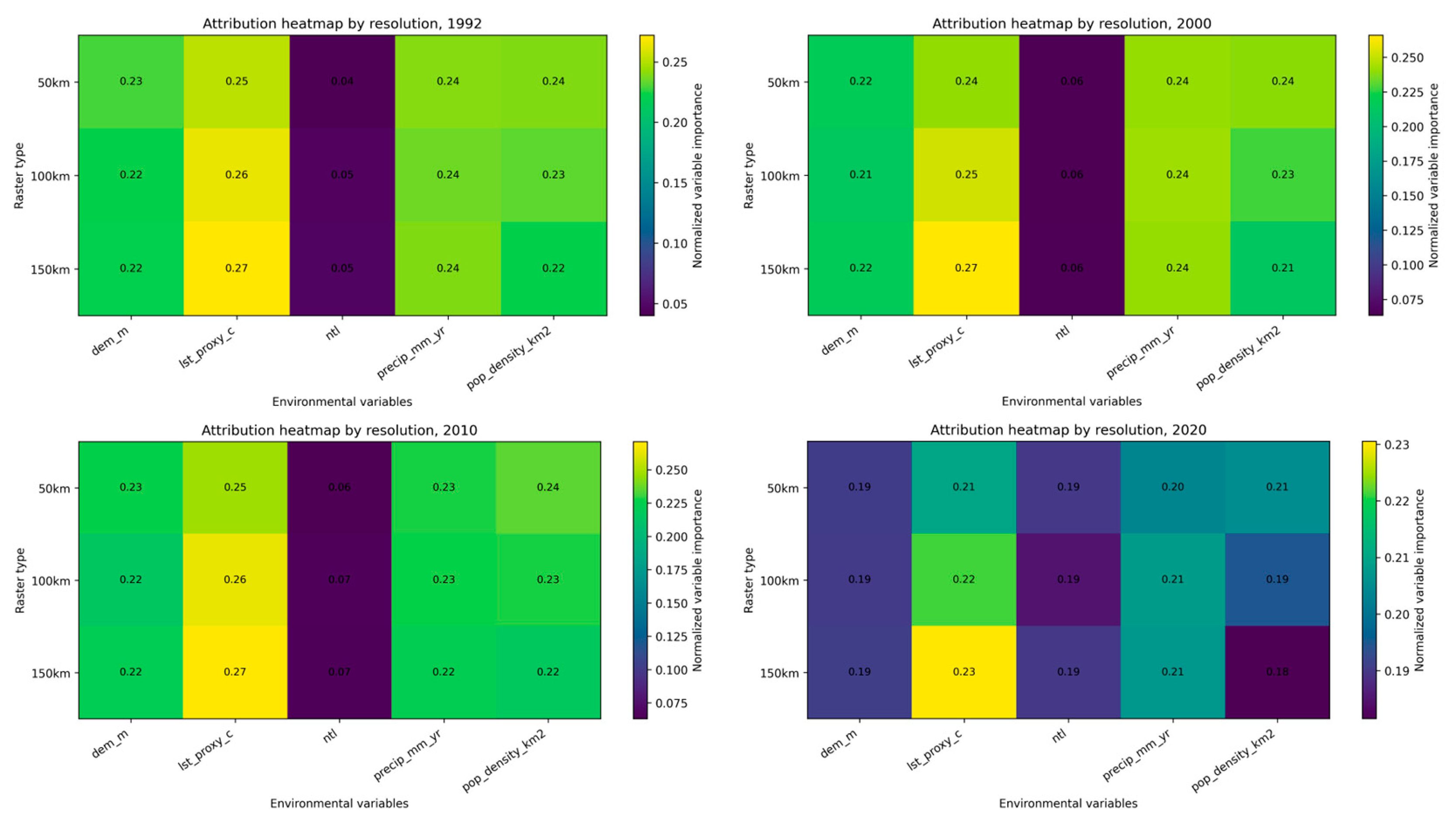
The spatial attribution results further demonstrate this coupled mechanism. During 1992–2010, the surface-temperature proxy generally showed the highest relative importance, with values of approximately 0.24–0.27, while precipitation remained relatively stable at approximately 0.22–0.24. These findings suggest that heat and moisture conditions form the persistent environmental background of border land transformation by influencing agricultural suitability, vegetation productivity, water availability, and ecosystem stability (Figure 11).

Population density exhibited greater importance within the 50 km zone than within the wider buffers, indicating that settlement growth, infrastructure development, and localized land demand are concentrated near accessible border sections. By contrast, the importance of climatic factors became more apparent at broader scales, where regional agricultural and ecological systems dominate. The contribution of NDVI increased substantially by 2020, reaching approximately 0.19, suggesting that vegetation response, ecological restoration, and natural succession became increasingly important in the later stage.

These results indicate a gradual shift from a driver structure dominated by a limited number of climatic and human factors toward a more balanced interaction among climate, vegetation, and socioeconomic activity. However, the attribution values represent relative explanatory importance rather than causal effects. A high contribution does not indicate whether a factor promotes or constrains land conversion, and the direction of influence may vary among climatic zones and development contexts.

3.4.3. Socioeconomic Drivers and Spatial Heterogeneity

The socioeconomic regression provides quantitative evidence that land-use change is associated with economic development and human-activity intensity. Within the 50 km analytical zone, the average cumulative land-use change ratio during 2000–2020 was 0.0186, while the maximum reached 0.1211, indicating that global averages conceal a limited number of highly active regions (

Table 4. OLS regression results of driving factors of land use change in 50 km buffer zone from 2000 to 2020.

Variable	Model (1)	Model (2)	Model (3)	Model (4)
POP_chg	0.0028	0.0018	0.0008	0.0013
	(0.0017)	(0.0016)	(0.0017)	(0.0016)
GDP_chg	0.0055 ***	0.0029 ***	0.0035 ***	0.0020 *
	(0.0011)	(0.0011)	(0.0011)	(0.0011)
NTL_chg	0.0305 ***	0.0131	0.0287 ***	0.0116
	(0.0090)	(0.0087)	(0.0085)	(0.0089)
Maritime Frontier		−0.0105 ***		−0.0094 ***
		(0.0014)		(0.0014)
Island		−0.0199 ***		−0.0176 ***
		(0.0015)		(0.0016)
North America			−0.0101 ***	−0.0075 ***
			(0.0013)	(0.0012)
Europe			0.0043 ***	0.0013
			(0.0015)	(0.0014)
Africa			0.0088 ***	0.0015
			(0.0020)	(0.0019)
South America			−0.0021	−0.0029
			(0.0025)	(0.0022)
Oceania			−0.0086 ***	−0.0032 *
			(0.0020)	(0.0019)
Constant term	0.0135 ***	0.0266 ***	0.0151 ***	0.0271 ***
	(0.0008)	(0.0015)	(0.0013)	(0.0018)
Frontier type control	No	Yes	No	Yes
Continental control	No	No	Yes	Yes
Sample Size	959	959	959	959
R2	0.077	0.284	0.180	0.307
Adjusted R2	0.074	0.281	0.172	0.299

Note: * and *** indicates the degree of significance of the relationship.

).

In the baseline model, GDP change and nighttime-light change were both positively associated with land-use change at the 1% significance level. These relationships are consistent with the effects of industrial expansion, infrastructure investment, settlement development, and increasing commercial activity. Population-density change was positive but insignificant, suggesting that demographic change does not exert a uniform independent influence at the global scale. Its effects may instead be mediated by economic development, urbanization, migration, and changes in production systems.

After spatial-environment type and continental context were included, the explanatory power of the model increased substantially. The fully adjusted model explained 30.7% of the variation in land-use change. GDP change retained a positive association, although only at the 10% significance level, while nighttime-light and population changes became insignificant. This weakening suggests that the relationships between socioeconomic development and land conversion are conditioned by geographical context.

Relative to international land borderlands, continental coastal margins and island margins exhibited significantly lower cumulative land-change ratios. These coefficients reveal persistent structural differences among the three spatial environments but should not be interpreted as direct evidence of specific mechanisms. International land borders are influenced by bilateral accessibility, land transport, agricultural development, and institutional discontinuity, whereas coastal and island margins are more strongly constrained by shoreline morphology, land availability, port accessibility, and environmental exposure.

Continental effects were also sensitive to model specification. Europe and Africa showed positive coefficients in the continent-controlled model, but these effects disappeared after type and socioeconomic variables were simultaneously considered. Therefore, broad interpretations such as “institution-driven European renewal” or “continent-driven African land transformation” are not sufficiently supported by the regression. The results instead indicate that economic change, human activity, spatial-environment type, and regional context jointly shape land-use heterogeneity.

4. Discussion

4.1. Scale-Dependent Boundary Effects and Natural–Social Dynamics

The decline in weighted transition intensity from the 50 km to the 150 km analytical zone indicates a general distance-decay pattern. This result is consistent with cross-border land-use studies showing that landscape disturbance is frequently concentrated around accessible crossings, settlements, transport corridors, and conflict-affected boundary sections [1,26]. However, approximately one-third of the analytical units exhibited an inverse scale effect. This finding extends previous research by demonstrating that major land transformations may occur in hinterland cities, agricultural frontiers, or regional infrastructure corridors rather than immediately adjacent to the boundary. The border effect should therefore be interpreted as a scale-dependent spatial association rather than a fixed zone ending at a uniform distance.

The attribution analysis further shows that the dominant explanatory structure changes with scale. Population density was more influential within the 50 km zone, consistent with evidence of continuing population concentration in global borderlands [26]. In contrast, temperature and vegetation variables became more important within the wider buffers, indicating that regional climatic and ecological systems increasingly shape the observed land transitions. This pattern supports the land-system science perspective that land change emerges from interactions among local human pressure, regional environmental conditions, institutional arrangements, and distant economic drivers [6,7,27].

The three buffers should therefore be treated as complementary analytical windows. The 50 km zone is most sensitive to localized development and infrastructure, the 100 km zone captures intermediate settlement and corridor processes, and the 150 km zone increasingly reflects regional climatic, ecological, and economic systems. These scales are not universal thresholds of border influence. They reveal different components of the border–hinterland system and are subject to scale dilution and spatial aggregation effects.

A conceptual distinction remains necessary. Political-geographical border effects apply most directly to international land borders, where sovereign institutions regulate mobility, development, and resource use [3,5,8,9]. Coastal and island gradients are more appropriately interpreted as land–sea interface and spatial-confinement effects, as emphasized in reviews of coastal and island land-cover change [14]. Comparing the three environments is analytically useful, but their similar spatial gradients should not be interpreted as evidence of identical causal mechanisms.

4.2. Data Resolution and High-Resolution Validation

The ESA Climate Change Initiative land-cover product provides a globally consistent annual record at 300 m resolution for 1992–2020 [28]. This temporal consistency supports long-term global comparison, but the spatial grain limits the detection of fragmented and linear border development. A 300 m pixel covers approximately 9 ha and may fail to identify narrow roads, checkpoints, railway corridors, warehouses, small settlements, and dispersed industrial facilities. Mixed pixels may consequently underestimate artificial surfaces, delay the recorded timing of conversion, and smooth localized high-value clusters.

The influence of resolution differs among indicators. Built-up SLUDD and built-up-related ALTR are particularly sensitive because errors affect both initial built-up area and converted area. ILUDD and W may underestimate turnover when several fine-scale transitions occur within a single pixel. Large-area transitions among forest, cropland, grassland, and bare land are expected to be comparatively more robust. Coastal and island environments are additionally affected by land–water mixing and coastline-position uncertainty, which are recognized challenges in remote-sensing analyses of land–sea margins [15].

Future research should adopt a nested multi-resolution framework. The ESA CCI series can retain its role as the globally consistent temporal backbone, while 10–30 m imagery can support regional change detection. Metre-scale products can then be used for local hotspot validation. SinoLC-1 provides a 1 m national land-cover map for China [29], while SinoBF-1 identifies building functions across major Chinese cities [30]. These datasets cannot replace the global time series because their temporal and geographic coverage differs, but they can improve the detection of fragmented artificial surfaces, assess hotspot displacement, and distinguish residential, industrial, commercial, transport, and public-service development.

4.3. Temporal Coverage, Scale Uncertainty, and Earth-Science Significance

The analysis ends in 2020 because the ESA CCI product used in this study provides a consistent annual global land-cover series from 1992 to 2020 [28]. The benchmark years 1992, 2000, 2010, and 2020 form three approximately decadal observation intervals and reduce the influence of short-term fluctuations. These intervals should not be interpreted as universally synchronous stages of border development. Regional transformations may have occurred before 1992 or may continue after 2020.

Scale-related uncertainty arises from buffer expansion, spatial aggregation, and analytical-unit delineation. Wider buffers may dilute localized boundary-proximate changes by incorporating stable hinterland areas, while large segments may conceal fine-scale hotspots. Conversely, broader buffers may reveal land transformations driven by regional cities, agricultural frontiers, or ecological systems. These results are consistent with land-system research emphasizing that local land changes are often connected to distant socioeconomic and environmental processes [6,27].

From an Earth-science perspective, border-related land change forms part of the coupled human–Earth system. Land-cover transitions affect carbon storage, surface albedo, evapotranspiration, runoff, habitat connectivity, and ecosystem services [6]. Border regions are particularly relevant because spatially continuous ecological processes intersect with discontinuous political and institutional systems. The framework developed here helps connect localized human disturbance with wider agricultural, climatic, and ecological processes and provides spatial evidence for transboundary forest protection, wetland conservation, carbon management, and biodiversity monitoring.

4.4. Limitations and Future Research

Several limitations should be acknowledged. First, international land borders, coastal margins, and island margins do not share identical institutional or environmental mechanisms. The present comparison identifies broad differences among territorial edge environments but cannot replace historically, politically, and ecologically grounded border typologies [5,8,9,14].

Second, land-cover aggregation and spatial resolution introduce classification uncertainty, particularly in fragmented built-up areas and land–water interfaces [14,28]. Future studies should incorporate classification accuracy into transition estimates and use high-resolution reference data to quantify uncertainty [29,30].

Third, the regression identifies statistical associations rather than causal effects. Border openness, bilateral trade, transport connectivity, governance quality, conflict exposure, port accessibility, and geopolitical risk were not directly measured. The significant type and continental coefficients therefore represent residual structural heterogeneity rather than direct evidence of specific institutional mechanisms.

Fourth, the socioeconomic regression was estimated only for the 50 km zone. Future research should construct multiscale spatial panel models and test interactions between buffer distance and driving factors. Moran’s I, spatial-error models, spatial-lag models, or spatial Durbin models should be considered where residual spatial dependence is significant.

Future work should combine longer time series, higher-resolution land-cover data, institutional and infrastructural variables, and explicit uncertainty analysis. These developments would shift the framework from global pattern identification toward a more comprehensive explanation of how environmental change, regional development, and territorial institutions jointly shape border land systems.

5. Conclusions

This study provides a global, multi-scale assessment of border land use change from 1992 to 2020, revealing consistent patterns, scale effects, and typology-dependent mechanisms that reshape the understanding of border land systems.

The main conclusions are as follows: (1) Boundary effects are scale-dependent and spatially clustered rather than uniformly distributed. While transition intensity decreases with increasing buffer distance, the relative ranking of active boundary segments remains stable, indicating that land use change is concentrated in a limited number of high-activity boundaries. Scale thus functions as a key dimension shaping the observable expression of border dynamics. (2) Global border land systems are governed by a dual-track dynamic of urban expansion and ecological restoration. Built-up land expansion—particularly during 2000–2010—coexists with widespread vegetation recovery and cropland-to-forest conversion, reflecting the combined influence of globalization, infrastructure development, and increasing ecological regulation. (3) The three analytical environment groups exhibit distinct transition structures and spatial associations, although the institutional and geopolitical mechanisms underlying these differences remain to be directly tested. Terrestrial, coastal, and island borders exhibit differentiated transition structures and evolutionary pathways, while three representative archetypes—forest frontier, agricultural expansion, and land–sea corridor—capture the dominant modes of global border land transformation. (4) Border land systems are transitioning from extensive, high-intensity restructuring to localized, incremental adjustment. Overall transition intensity declines over time, while land use change becomes increasingly concentrated in corridor and node-like segments, indicating a shift toward more stable and regulated land system dynamics. (5) A limited number of high-contribution boundary segments act as critical nodes of land system transformation. These “hotspot boundaries” dominate global transition intensity and represent priority targets for spatial governance and risk management.

From a policy perspective, these findings highlight the need to move beyond uniform border management toward targeted, scale-sensitive strategies. High intensity boundary segments require coordinated cross-border governance and risk control, while low-intensity regions should prioritize ecological stability and long-term monitoring. More broadly, integrating boundary effects with regional development and ecological processes provides a more effective framework for sustainable land management in border regions.

References

1. Basse, R.M.; Omrani, H.; Charif, O.; Gerber, P.; Bódis, K. Land Use Changes Modelling Using Advanced Methods: Cellular Automata and Artificial Neural Networks. The Spatial and Explicit Representation of Land Cover Dynamics at the Cross-Border Region Scale. Appl. Geogr. 2014, 53, 160–171. [Google Scholar] [CrossRef] [Scilit]
2. Castanho, R.A.; Behradfar, A. Cross-Border Cooperation and Land-Use: Studying Two European Cities in the Period 2000–2018. J. Borderl. Stud. 2024, 40, 1157–1176. [Google Scholar] [CrossRef] [Scilit]
3. Sohn, C. Modelling Cross-Border Integration: The Role of Borders as a Resource. Geopolitics 2014, 19, 587–608. [Google Scholar] [CrossRef] [Scilit]
4. Peters, R.; Ripple, W.J.; Wolf, C.; Moskwik, M.; Carreón-Arroyo, G.; Ceballos, G.; Córdova, A.; Dirzo, R.; Ehrlich, P.R.; Flesch, A.D.; et al. Nature Divided, Scientists United: US–Mexico Border Wall Threatens Biodiversity and Binational Conservation. BioScience 2018, 68, 740–743. [Google Scholar] [CrossRef] [Scilit]
5. Newman, D. The Lines That Continue to Separate Us: Borders in Our “Borderless” World. Prog. Hum. Geogr. 2006, 30, 143–161. [Google Scholar] [CrossRef] [Scilit]
6. Turner, B.L.; Lambin, E.F.; Reenberg, A. The Emergence of Land Change Science for Global Environmental Change and Sustainability. Proc. Natl. Acad. Sci. USA 2007, 104, 20666–20671. [Google Scholar] [CrossRef] [Scilit] [PubMed]
7. Turner, B.L.; Meyfroidt, P.; Kuemmerle, T.; Müller, D.; Chowdhury, R.R. Framing the Search for a Theory of Land Use. J. Land Use Sci. 2020, 15, 489–508. [Google Scholar] [CrossRef] [Scilit]
8. Brunet-Jailly, E. Theorizing Borders: An Interdisciplinary Perspective. Geopolitics 2005, 10, 633–649. [Google Scholar] [CrossRef] [Scilit]
9. Paasi, A. Boundaries as Social Processes: Territoriality in the World of Flows. Geopolitics 1998, 3, 69–88. [Google Scholar] [CrossRef] [Scilit]
10. Fowler, N.; Keitt, T.; Schmidt, O.; Terry, M.; Trout, K. Border Wall: Bad for Biodiversity. Front. Ecol. Environ. 2018, 16, 137–138. [Google Scholar] [CrossRef] [Scilit]
11. Zheng, F.; Xiao, C.; Feng, Z. Impact of Armed Conflict on Land Use and Land Cover Changes in Global Border Areas. Land Degrad. Dev. 2023, 34, 873–884. [Google Scholar] [CrossRef] [Scilit]
12. Eurostat, P. Farms and Farmland in the European Union-Statistics 2022. Available online: https://ec.europa.eu/eurostat/statistics-explained/index.php (accessed on 10 March 2026).
13. Vu, H.T.D.; Tran, D.D.; Schenk, A.; Nguyen, C.P.; Vu, H.L.; Oberle, P.; Trinh, V.C.; Nestmann, F. Land Use Change in the Vietnamese Mekong Delta: New Evidence from Remote Sensing. Sci. Total Environ. 2022, 813, 151918. [Google Scholar] [CrossRef] [Scilit] [PubMed]
14. Tiengo, R.; Palacios-Orueta, A.; Uchôa, J.; Gil, A. Remote Sensing Approaches for Land Use/Land Cover Change Detection in Coastal Areas and Oceanic Islands: A Systematic Review. J. Integr. Coast. Zone Manag. 2023, 23, 153–175. [Google Scholar] [CrossRef] [Scilit]
15. GADM. Database of Global Administrative Areas, Version 4.1. Available online: https://gadm.org/ (accessed on 10 March 2026).
16. Earth, N. Natural Earth Data: 1:10m Physical Vectors—Coastline and Land. Available online: https://www.naturalearthdata.com/ (accessed on 10 March 2026).
17. Wang, X.; Bao, Y. Study on the Methods of Land Use Dynamic Change Research. Prog. Geogr. 1999, 18, 83–89. [Google Scholar]
18. Xiao, X.; Huang, X.; Jiang, L.; Jin, C. Empirical Study on Comparative Analysis of Dynamic Degree Differences of Land Use Based on the Optimization Model. Geocarto Int. 2022, 37, 9847–9864. [Google Scholar] [CrossRef] [Scilit]
19. Zhou, G.; Long, H. Mechanism of Land Use Transition and Territorial Spatial Pattern Optimization: Analysis from the Perspective of Spatial Function of Land Use Benefit. J. Nat. Resour. 2023, 38, 2447–2463. [Google Scholar] [CrossRef] [Scilit]
20. Thorson, J.T.; Andrews, A.G.; Essington, T.E.; Large, S.I. Dynamic Structural Equation Models Synthesize Ecosystem Dynamics Constrained by Ecological Mechanisms. Methods Ecol. Evol. 2024, 15, 744–755. [Google Scholar] [CrossRef] [Scilit]
21. Basu, T.; Das, A. Urbanization Induced Changes in Land Use Dynamics and Its Nexus to Ecosystem Service Values: A Spatiotemporal Investigation to Promote Sustainable Urban Growth. Land Use Policy 2024, 144, 107239. [Google Scholar] [CrossRef] [Scilit]
22. Liu, J.; Liu, M.; Tian, H.; Zhuang, D.; Zhang, Z.; Zhang, W.; Tang, X.; Deng, X. Spatial and Temporal Patterns of China’s Cropland during 1990–2000: An Analysis Based on Landsat TM Data. Remote Sens. Environ. 2005, 98, 442–456. [Google Scholar] [CrossRef] [Scilit]
23. Wu, Y.; Zhou, C.; Lai, X.; Li, Y.; Miao, L.; Yu, H. Spatio-Temporal Characteristics and Decoupling Relationship of New-Type Urbanization and Carbon Emissions at the County Level: A Case Study of Zhejiang Province, China. Ecol. Indic. 2024, 160, 111793. [Google Scholar] [CrossRef] [Scilit]
24. Cui, X.; Guo, Y. Analysis on Spatiotemporal Dynamic Evolution of Land Use Structure of Urban Agglomerations in Western China in Recent 40 Years. J. Arid Land Resour. Environ. 2022, 36, 16–24. [Google Scholar] [CrossRef]
25. Elvidge, C.D.; Imhoff, M.L.; Baugh, K.E.; Hobson, V.R.; Nelson, I.; Safran, J.; Dietz, J.B.; Tuttle, B.T. Night-Time Lights of the World: 1994–1995. J. Photogramm. Remote Sens. 2001, 56, 81–99. [Google Scholar] [CrossRef] [Scilit]
26. Xiao, C.; Feng, Z.; You, Z.; Zheng, F. Population Boom in the Borderlands Globally. J. Clean. Prod. 2022, 371, 133685. [Google Scholar] [CrossRef] [Scilit]
27. Meyfroidt, P.; Lambin, E.F.; Erb, K.-H.; Hertel, T.W. Globalization of Land Use: Distant Drivers of Land Change and Geographic Displacement of Land Use. Curr. Opin. Environ. Sustain. 2013, 5, 438–444. [Google Scholar] [CrossRef] [Scilit]
28. European Space Agency. ESA Climate Change Initiative Land Cover Data: Annual Global Land-Cover Maps at 300 m Resolution. Available online: https://climate.esa.int/en/projects/land-cover/ (accessed on 22 December 2025).
29. Li, Z.; He, W.; Cheng, M.; Hu, J.; An, X.; Huang, Y.; Yang, G.; Zhang, H. SinoLC-1: The First 1 m Resolution National-Scale Land-Cover Map of China Created with a Deep Learning Framework and Open-Access Data. Earth Syst. Sci. Data 2023, 15, 4749–4780. [Google Scholar] [CrossRef] [Scilit]
30. Li, Z.; Li, L.; Hu, T.; Cheng, M.; He, W.; Qiu, T.; Zhang, L.; Zhang, H. Satellite Mapping of Every Building’s Function in Urban China Reveals Deep Built Environment Disparities. Nat. Commun. 2026, 17, 2827. [Google Scholar] [CrossRef] [Scilit] [PubMed]
Figure 1. The frontier types (a) and the national boundaries of six continents (b) used in this study.
Land 15 01485 g001
Figure 2. The land cover type is based on the 2020 global border area land use (300 m × 300 m) map under the 50 km buffer zone reclassified and standardized by globeland30 (a), and the three colors represent the buffer zone with three scales of 50 km (b), 100 km (c) and 150 km (d) respectively.
Land 15 01485 g002
Figure 3. Research framework of this study.
Land 15 01485 g003
Figure 4. Distribution of ALTR index in different types of frontiers under 50 km (a), 100 km (b) and 150 km (c) buffer zone scales from 1992 to 2020.
Land 15 01485 g004
Figure 5. Comparison of area retention rate and SLUDD index of different land use types in different periods under three buffer zone scales: (a) borderland under 50 km, (b) coastal areas and territorial seas under 50 km, (c) island territory under 50 km, (d) borderland under 100 km, (e) coastal areas and territorial seas under 100 km, (f) island territory under 100 km, (g) borderland under 150 km, (h) coastal areas and territorial seas under 150 km, and (i) island territory under 150 km.
Land 15 01485 g005
Figure 6. Analysis of land use transfer under three buffer zone scales in different periods: (a) 50 km buffer in T0, (b) 100 km buffer in T0, (c) 150 km buffer in T0, (d) 50 km buffer in T1, (e) 100 km buffer in T1, (f) 150 km buffer in T1, (g) 50 km buffer in T2, (h) 100 km buffer in T2, (i) 150 km buffer in T2, (j) 50 km buffer in T3, (k) 100 km buffer in T3, and (l) 150 km buffer in T3. T0 denotes the full study period (1992–2020).
Land 15 01485 g006
Figure 7. Changes in SLUDD and ILUDD of global land use from 1992 to 2020: (a) SLUDD under 50 km buffer, (b) SLUDD under 100 km buffer, (c) SLUDD under 150 km buffer, (d) ILUDD under 50 km buffer, (e) ILUDD under 100 km buffer, and (f) ILUDD under 150 km buffer.
Land 15 01485 g007
Figure 8. Comparison of land use transfer area and ALTR index under different buffer zone scales across continents: (a) 50 km buffer in T0, (b) 100 km buffer in T0, (c) 150 km buffer in T0, (d) 50 km buffer in T1, (e) 100 km buffer in T1, (f) 150 km buffer in T1, (g) 50 km buffer in T2, (h) 100 km buffer in T2, (i) 150 km buffer in T2, (j) 50 km buffer in T3, (k) 100 km buffer in T3, and (l) 150 km buffer in T3 (Note: the left vertical axis is the proportion of transferred area, the right vertical axis is the ALTR index, and the horizontal axis shows the continents).
Land 15 01485 g008
Figure 9. Five-level zoning maps of the W index in the global boundary buffer zones at 50 km (a), 100 km (b) and 150 km (c), and the selection of key areas.
Land 15 01485 g009
Figure 10. Differences in the proportion of land use transfer at the boundaries of different regions under the same buffer zone scale in the global border areas (a,b) from 1992 to 2020, (c,d) from 1992 to 2000, and (e,f) from 2000 to 2010. (Note: The Nightingale rose chart on the left refers to the national differences in all borders, while the stacked bar chart on the right shows some typical examples. The two-letter country code of the international standards organization (IOS) in the stacked bar chart represents the boundary between the two countries, and null represents the sea area. For example, bra-col and cnn-null are the boundaries between Brazil and Colombia and the coast of China.
Land 15 01485 g010
Figure 11. Thermodynamic diagram of natural and socio-economic drivers.
Land 15 01485 g011