Article

Spatiotemporal Evolution and Hotspot Transitions of Eco-Environmental Quality in the Yellow River Basin: Evidence from Ecological Restoration Projects

1
School of Geography and Environment, Liaocheng University, Liaocheng 252000, China
2
Institute of Huanghe Studies, Liaocheng University, Liaocheng 252000, China
3
National Ecosystem Science Data Center, Key Laboratory of Ecosystem Network Observation and Modeling, Institute of Geographic Sciences and Natural Resources Research, Chinese Academy of Sciences, Beijing 100101, China
4
Comprehensive Survey Command Center for Natural Resources, China Geological Survey, Beijing 100055, China
5
Key Laboratory of Coupling Process and Effect of Natural Resources Elements, Ministry of Natural Resources, Beijing 100055, China
*
Author to whom correspondence should be addressed.
Land 2026, 15(8), 1379; https://doi.org/10.3390/land15081379
Submission received: 3 July 2026 / Revised: 28 July 2026 / Accepted: 29 July 2026 / Published: 31 July 2026

Abstract

The Yellow River Basin (YRB), a core ecological–economic corridor in China, plays a critical role in meeting climate, land, and water-related Sustainable Development Goals (SDGs). To capture the dynamic evolution of Eco-environmental Quality (EEQ), this study developed a process-oriented space-time cube framework based on the Remote Sensing Ecological Index (RSEI) using MODIS data from 2000 to 2021 on the Google Earth Engine (GEE) platform. By integrating Emerging Hotspot Analysis (EHSA) with the RSEI cube, we identified and tracked 17 EEQ hotspot–coldspot evolution types and revealed their spatial clustering, temporal persistence, and cumulative transition effects. The driving mechanisms were further investigated through a comprehensive analytical framework combining Geodetector (GD), Ordinary Least Squares (OLS), and Multiscale Geographically Weighted Regression (MGWR). Results show that: (1) the RSEI-based space–time cube effectively detects co-evolving hotspot–coldspot trajectories and uncovers fine-grained spatiotemporal instability across the basin; (2) dynamic hotspot types, including diminishing, oscillating, and sporadic patterns, occupy a larger proportion of the basin than persistent hotspots, indicating widespread ecological fluctuation; (3) hotspot transition analysis reveals that only 4.94% of the 17.04% emerging hotspots became stable from 2000 to 2010, to 2011 to 2021, while the majority remained transitional or reverted to coldspots, reflecting fragile early-stage ecological recovery; and (4) Fractional vegetation cover (FVC) exhibited the highest explanatory power for EEQ hotspot–coldspot transition dynamics, followed by topography and temperature, whereas anthropogenic factors exerted their influence primarily through interactions with natural factors. These findings provide a robust scientific basis for precision ecological restoration, risk identification in fragile ecological zones, and adaptive sustainable management of large river basins under complex environmental pressures.

1. Introduction

Ecological and environmental crises have become major threats to the sustainability of human civilization and global economic development [1,2]. The Yellow River Basin (YRB), a socio-ecological corridor critical to China’s sustainable development, faces ecological degradation that poses challenges to ecosystem stability, water security, and climate resilience [3,4]. In recent decades, a series of large-scale ecological restoration initiatives, such as the Three-North Shelter Forest Program, the Grain-for-Green Project, and the YRB Ecological Protection and High-Quality Development Strategy, have been implemented throughout the region [5]. Ecological change detection has become a central topic in environmental remote sensing, aiming to understand the spatiotemporal dynamics of Eco-environmental Quality (EEQ) under long-term environmental and anthropogenic influences [6]. Although research on EEQ in the YRB has expanded considerably, systematic investigations into the evolutionary types and transformation trajectories of EEQ hotspots and coldspots remain scarce. This limitation constrains a holistic understanding of ecological transition mechanisms and the spatial relationships between ecological restoration initiatives and EEQ dynamics. Previous studies in the YRB have extensively investigated ecological changes using remote sensing-based ecological indices, spatiotemporal trend analysis, and driving factor assessment [7]. These studies have provided valuable insights into the overall improvement of ecological quality associated with ecological restoration programs, while also revealing strong spatial heterogeneity driven by climate variability, topographic gradients, land use changes, and human activities [8,9,10]. However, most existing studies have primarily focused on describing ecological status or overall temporal trends, with limited attention to the dynamic transition processes, persistence, and migration pathways of ecological improvement and degradation.
Traditional EEQ assessment methods, including bi-temporal comparisons, time-series modeling, and spatial hotspot analysis, typically examine temporal and spatial dimensions separately. This separation constrains their ability to capture continuous ecological processes and cross-scale interactions [11,12,13]. Bi-temporal approaches provide only coarse snapshots, whereas time-series models emphasize temporal patterns but often neglect spatial dependencies. In addition, spatial hotspot detection methods commonly overlook temporal continuity. As a result, these decoupled approaches fail to represent the interactive spatiotemporal processes that underpin ecological dynamics in large basins [14]. In contrast, spatiotemporal data mining based on the space-time cube (STC) provides a unified three-dimensional framework that integrates spatial and temporal information within a single analytical structure, thereby improving computational efficiency and enabling systematic extraction of spatiotemporal patterns [15,16,17]. By converting irregular time series into standardized temporal bins, the STC enhances analytical robustness and supports consistent comparison across space and time [18]. It also accommodates advanced quantitative analyses, automated pattern detection, and the integration of multisource data through clustering techniques [19,20]. When applied to the Remote Sensing Ecological Index (RSEI), the STC framework simultaneously characterizes spatial configuration and temporal evolution, enabling the detection of co-evolution patterns and the systematic tracking of EEQ hotspot and coldspot transitions. This approach facilitates the identification of diverse evolution types such as emerging, persistent, sporadic, and oscillating patterns, which traditional methods often fail to capture. Overall, STC-based spatiotemporal analysis provides an efficient and comprehensive pathway for revealing complex EEQ dynamics that are essential for basin-scale environmental assessment and management. The YRB provides a particularly suitable setting for this analysis because its pronounced climatic, topographic, land-use, and anthropogenic gradients, together with extensive ecological restoration interventions, allow ecological transition trajectories to be examined across highly heterogeneous environmental contexts within a single large river basin.
The RSEI has become one of the most widely applied indicators for assessing EEQ because it integrates greenness, humidity, dryness, and heat into a single, analytically robust metric [21]. Its simple structure, reliance on multisource satellite data, and compatibility with automated computation platforms such as Google Earth Engine(GEE) enable efficient long-term and basin-scale ecological monitoring [22,23]. Existing studies across diverse landscapes have demonstrated that the standard RSEI framework provides consistent performance in regions characterized by complex geomorphology, making it particularly suitable for large and heterogeneous basins such as the Yellow River Basin [24]. These advantages establish RSEI as a reliable basis for spatiotemporal analysis and support its integration into advanced analytical frameworks that aim to capture ecological evolution processes rather than static patterns. Meanwhile, other remote sensing-based composite indices have been developed to characterize specific ecological functions, such as ecosystem productivity or habitat dynamics, by incorporating additional environmental and land-surface variables [25,26,27]. Compared with these indices, RSEI is particularly suitable for this study because our objective is to evaluate overall EEQ and identify long-term spatiotemporal transition trajectories rather than quantify a single ecosystem function.
Research on the drivers of EEQ has increasingly relied on statistical and spatial analytical approaches, including correlation analysis [28], Geodetector (GD) [29,30], geographically weighted regression (GWR) [31], and machine learning [32,33]. These methods have revealed the influence of both natural and anthropogenic factors such as climate [34,35], topography, land use, and socioeconomic conditions [36,37]. However, existing studies have often addressed driver interactions and spatial heterogeneity separately, making it challenging to simultaneously characterize how multiple factors interact and vary spatially across large heterogeneous basins [24,38,39]. GD can quantify interaction strengths but lacks the capacity to model spatially varying relationships, whereas GWR and its multiscale extensions address spatial heterogeneity but only partially reflect factor interactions. Machine learning models are capable of detecting nonlinear relationships, yet their limited interpretability restricts their application in policy-oriented ecological research. These methodological limitations result in an incomplete characterization of the coupled interaction–heterogeneity mechanisms driving EEQ change, particularly in large and spatially diverse river basins. These gaps highlight the need for integrated analytical frameworks capable of representing both heterogeneous spatial processes and complex driver interactions. In this study, the combined use of GD, Multiscale Geographically Weighted Regression (MGWR), and Ordinary Least Squares (OLS) enables a more comprehensive exploration of the multiscale mechanisms shaping RSEI hotspot–coldspot transitions.
China has implemented a suite of large-scale ecological restoration and environmental management programs in the Yellow River Basin, including the Grain for Green Program, the Three-North Shelterbelt Project, basin-wide soil and water conservation initiatives, and ecological protection measures under the Yellow River Basin Ecological Protection and High-Quality Development Strategy [40]. These interventions have collectively improved vegetation conditions and reduced soil erosion across extensive areas of the basin. However, ecological responses remain highly heterogeneous and often display phased, lagged, or even reversible patterns due to the basin’s complex climatic gradients, geomorphological diversity, and intensive human–environment interactions [41,42,43]. Existing research has primarily focused on specific subregions or individual indicators, offering limited understanding of basin-wide spatiotemporal dynamics of EEQ hotspots and coldspots. Moreover, few studies have examined the coupled temporal evolution and spatial heterogeneity that shape hotspot-coldspot trajectories, leaving critical transformation types and transition zones insufficiently characterized [44]. These limitations hinder the diagnosis of underlying ecological drivers and constrain evidence-based basin management. A systematic framework capable of jointly capturing spatiotemporal evolution and its driving mechanisms is therefore urgently needed.
Overall, existing studies on EEQ have predominantly focused on ecological status assessment and trend evaluation, while comparatively less attention has been paid to the dynamic transition processes underlying ecological change. As a result, the spatiotemporal evolution, persistence, and migration of ecological hotspots and coldspots remain insufficiently understood. To enhance the identification of dynamic processes governing EEQ evolution, this study integrates hotspot–coldspot trajectory analysis into an RSEI-based space–time cube (STC) framework. Rather than introducing a new methodological algorithm, this study develops a process-oriented analytical framework that links EEQ evolution trajectories with hotspot-coldspot transition dynamics and their spatially heterogeneous driving mechanisms across space and time. Each analytical component addresses a distinct level of ecological inquiry, progressing from EEQ characterization (RSEI), to hotspot–coldspot evolution (STC–EHSA), driver identification (GD), and spatially heterogeneous response analysis (MGWR). Specifically, this study aims to (1) identify the spatiotemporal evolution patterns and transition trajectories of EEQ hotspots and coldspots across the Yellow River Basin; (2) quantify the dominant natural and anthropogenic drivers and reveal their spatially heterogeneous effects on EEQ evolution; and (3) evaluate the spatial correspondence between ecological restoration projects and EEQ improvement hotspots to provide insights into ecological restoration assessment and sustainable basin management. Moving beyond conventional static assessments, the proposed framework captures the temporal continuity, accumulation effects, and transition pathways associated with ecological improvement and degradation, thereby revealing long-term evolutionary trajectories of ecological quality. Furthermore, the combined application of GD, OLS, and MGWR enables a comprehensive examination of the driving factors and their spatially heterogeneous effects on hotspot–coldspot formation and migration. By linking EEQ evolution with hotspot–coldspot transition dynamics and spatially differentiated driving mechanisms, this study provides a process-oriented perspective for understanding EEQ change across the Yellow River Basin. Although developed for the YRB, the proposed process-oriented framework can be transferred to other large and heterogeneous river basins or regions undergoing ecological restoration, where identifying ecological trajectories and their driving mechanisms is essential for adaptive ecosystem management.

2. Materials and Methods

2.1. Study Area

The Yellow River is the fifth longest river globally and serves as a critical water resource for northern China. The Yellow River originates from the northern slopes of the Bayan Har Mountains on the Qinghai–Tibet Plateau (Figure 1). It flows through nine provinces and autonomous regions, namely, Qinghai, Sichuan, Gansu, Ningxia, Inner Mongolia, Shanxi, Shaanxi, Henan, and Shandong, before finally discharging into the Bohai Sea. As one of China’s most important ecological security barriers, the YRB serves as a key region for human settlement, economic development, and social activities. It extends from west to east across four major geomorphic units—the Qinghai–Tibet Plateau, the Inner Mongolia Plateau, the Loess Plateau, and the Huang-Huai-Hai Plain—encompassing the three principal topographic steps of China. The drainage area covers 795,800 km2, representing approximately 8.3% of China’s total land area. The YRB is characterized by a continental climate, with distinct regional variations. The southeastern part experiences a semi-humid climate, the central region is dominated by a semi-arid climate, and the northwestern area is classified as arid. The primary land use types in the YRB include grassland, farmland, and forest, which account for 48.35%, 25.08%, and 13.46% of the total basin area, respectively. The YRB encompasses diverse and ecologically significant regions, including the Qinghai–Tibet Plateau characterized by harsh climatic conditions, the Loess Plateau marked by severe soil erosion, and the Kubuqi and Mu Us Deserts, which are frequently affected by wind and sand hazards. These ecosystems are highly sensitive and vulnerable to disturbances, making them prone to ecological degradation. Once ecological damage occurs, recovery is extremely difficult. Therefore, the region has long remained a focal point for ecological conservation and management in China.

2.2. Data Source and Processing Methodology

MODIS remote sensing datasets, including the MOD09A1 (Terra Surface Reflectance 8-Day Global 500 m), MOD11A2 (Terra Land Surface Temperature and Emissivity 8-Day Global 1 km), and MOD13A1 (Terra Vegetation Indices 16-Day Global 500 m) products, were utilized to calculate the RSEI over the peak vegetation growing season (July–September) from 2000 to 2021. The MOD09A1 product provides atmospherically corrected surface reflectance data. To improve data quality, the MOD09A1 StateQA quality assurance layer was used to mask pixels affected by clouds, cloud shadows, and cirrus contamination prior to image compositing. This period was selected to minimize the influence of seasonal variability and phenological differences and to improve the interannual comparability of EEQ assessments across the YRB. To ensure analytical accuracy and consistency, only imagery with less than 5% cloud cover was included. MODIS data products, acquired via GEE, were processed to derive the RSEI at a spatial resolution of 500 m. The study investigates the driving factors underlying the evolution of EEQ in the YRB, integrating both natural and anthropogenic variables, including DEM, slope, aspect, annual average precipitation (PRE), temperature (TEMP), topographic wetness index (TWI), terrain ruggedness index (TRI), fractional vegetation cover (FVC), population density (POP), gross domestic product (GDP), and land use/land cover (LULC). The resolutions and sources are presented in Table 1. Among these factors, slope, aspect, TWI, and TRI were primarily derived from DEM data. The formulas for the TWI and TRI are presented in Equations (1) and (2), respectively:
TWI   =   ln ( a tan β )
where a represents the water collection area per unit width, and β represents the slope angle.
TRI = 1 n i = 1 n ( h i h - ) 2
where n = 9, representing the number of neighboring pixels considered in the calculation. The variable i denotes the index of the neighboring pixel, where the elevation of the i - th adjacent pixel is compared with that of the central pixel. h i represents the elevation of adjacent pixels and h - represents the elevation of the central pixel.
To ensure consistency and compatibility for subsequent analyses, all datasets were standardized to a uniform coordinate system and resampled to a spatial resolution of 1000 m. For land use/land cover (LULC) data, a fractional one-hot encoding (soft classification) approach was adopted, whereby each land-use category was represented by its proportional occurrence within the resampled unit. No categorical threshold was applied, and all category proportions were retained as continuous variables, thereby preserving mixed land-cover composition and reducing information loss during resampling. The boundary datasets of the Sanjiangyuan Ecological Protection and Construction Project, the Grain for Green Program, and the Grazing Withdrawal Program were obtained from a previously published study and used for subsequent spatial analyses [45].
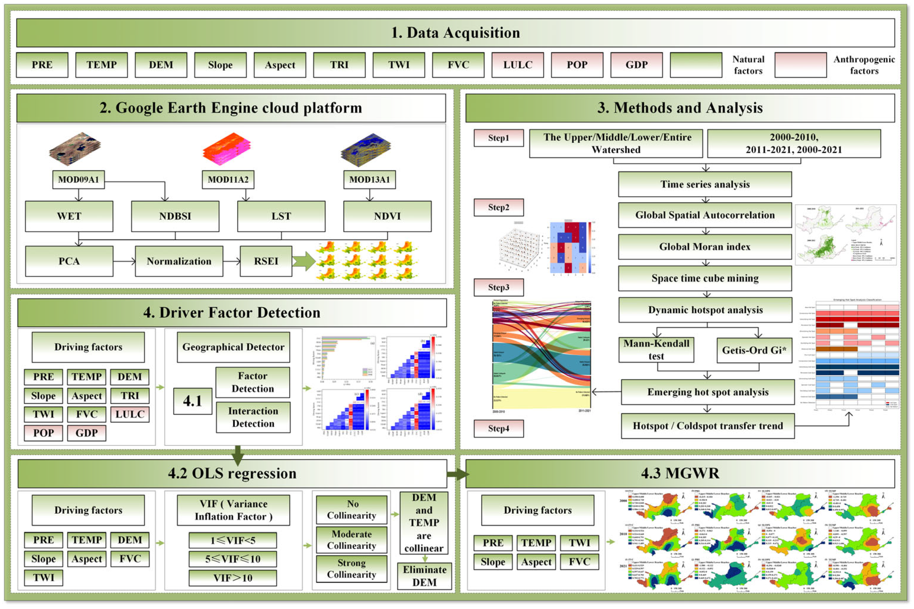
The overall research framework is illustrated in Figure 2. First, an annual RSEI dataset for the period 2000–2021 was constructed using the GEE platform. The Global Moran’s I index was then applied to test the spatial autocorrelation of the RSEI values; if significant spatial autocorrelation was detected, EHSA was subsequently conducted. Based on the RSEI time series, STC was constructed for the YRB, and the Mann–Kendall (MK) trend test and the Getis–Ord Gi* statistic were employed to identify the spatiotemporal evolution patterns of the EEQ hotspots and coldspots. To elucidate the drivers of hotspot–coldspot transitions, we employed a multi-model integration approach combining GD, OLS, and MGWR, incorporating natural factors such as temperature and topography alongside anthropogenic factors such as GDP.

2.3. RSEI Construction

The RSEI incorporates four essential ecological indicators: wetness (WET), normalized difference vegetation index (NDVI), land surface temperature (LST), and normalized difference built-up and soil index (NDBSI), which correspond to moisture, vegetation greenness, thermal conditions, and dryness, respectively. These indicators are standardized and synthesized through the first principal component (PC1) derived from principal component analysis (PCA), thereby offering an integrated evaluation of regional EEQ. The RSEI can be formulated as a function of four indicators: greenness, humidity, dryness, and heat, as presented in Formulas (3) and (4) [46]. To address the inconsistency in units and scales among the four ecological indicators, all variables were normalized to a uniform scale ranging from 0 to 1 prior to PCA. The normalization formula is presented in Equation (5). Following the PCA in Xu’s scheme [26], to ensure that a higher RSEI value reflects better EEQ, it must be determined whether Equation (4) should be applied based on the signs of the eigenvectors. If the eigenvector signs for greenness and humidity are positive while those for dryness and heat are negative, then no processing via Equation (4) is necessary. Finally, the resulting RSEI0 is normalized using Equation (6). The RSEI ranges from 0 to 1, with higher values indicating better ecological quality and lower values reflecting poorer ecological conditions. In this study, the EEQ of the YRB from 2000 to 2021 was analyzed using MODIS imagery. Preprocessing of the images involved radiometric correction, atmospheric correction, cropping, reprojection, and the masking of water bodies.
RSE I 0 = PC 1 ( WET , NDVI , LST , NDBSI )
RSE I 0 = 1   PC 1 ( WET , NDVI , LST , NDBSI )
where PC1 is the first principal component after the principal component analysis, and  RSE I 0 is the un-normalized raw RSEI. The calculation formulas for the WET, NDVI, LST, and NDBSI are presented in Supplementary Table S1. The results of the principal component analysis are shown in Supplementary Table S2. To ensure the temporal comparability and physical interpretability of the RSEI, PCA loading directions were examined for all study years (Supplementary Table S2). The results show that NDVI and wetness consistently exhibited positive loadings, whereas NDBSI and LST maintained negative loadings throughout 2000–2021, indicating stable physical meanings of the principal components over time. Therefore, no inversion of the raw RSEI was required.
Furthermore, the consistent loading directions of the four RSEI components and the relatively high contribution rate of PC1 across all years demonstrate the stability and temporal comparability of the RSEI, supporting its applicability for EEQ assessment in the Yellow River Basin.
  NI n = I n I min I max I min
In the formula, NI n is the normalized value of each index, I n is the value of each index at pixel n, I max represents the maximum value of each index, and I min represents the minimum value of each index.
RSEI = RSE I 0 RSEI min RSEI max + RSEI min
where RSEI max and RSEI min are the maximum value and the minimum value, respectively. RSE I 0 is the un-normalized raw RSEI. The results are shown in Supplementary Figure S1.

2.4. Spatial Autocorrelation Analysis

Spatial autocorrelation analysis was employed to assess whether the distribution of RSEI variables exhibited clustering patterns, encompassing both global and local autocorrelation. The Global Moran’s Index (Global Moran’s I) [47] was applied to assess the spatial autocorrelation of the RSEI values across grid cells within the YRB, aiming to identify significant spatial distribution patterns or clustering in EEQ. The Global Moran’s I ranges from –1 to 1, where positive values indicate spatial clustering, negative values suggest spatial dispersion, and values near zero imply random spatial distribution.
G l o b a l   M o r a n s   I = n i = 1 n j = 1 n W i j ( x i x ¯ ) ( x j x ¯ ) ( i = 1 n j = 1 n W i j ) i = 1 n ( x i x ¯ ) 2  
In Equation (7), W is the spatial matrix; n is the number of regional units; x i is the observed value of the i -th unit; x ¯ is the average value of the observations; and W i j is the spatial weight matrix of each unit.

2.5. OLS Regression Analysis

The OLS model is a classical linear regression technique used to estimate the optimal regression coefficients by minimizing the sum of squared differences between observed and predicted values, thereby capturing the global relationship between dependent and independent variables. The OLS model is defined using Equation (8) [48].
Y = α 0 + α 1 x 1 + α 2 X 2 + α 0 X 3 + . . . . . . . + α n X n + ϵ
where Y is the dependent variable, X is the independent variable, α is the regression coefficient, and ε is the error term.

2.6. STC and EHSA and RSEI-Based Ecological Index Cube

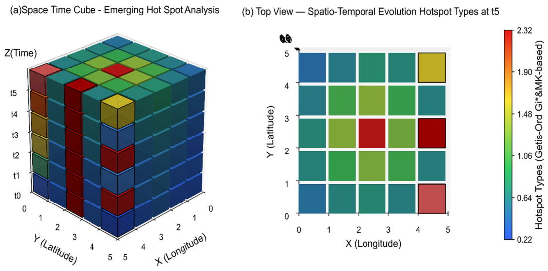
The STC model provides a unified analytical method for integrating spatial and temporal dimensions, overcoming the limitations of traditional spatial statistics that treat time as discrete or independent snapshots. Utilizing the STC method, each spatial unit is represented as a series of temporal bins stacked along the time axis, forming a three-dimensional cube, where the X–Y plane denotes the spatial distribution, and the Z-axis captures temporal progression (Figure 3a). Each cube represents a temporal slice, with newer timestamps on the top and older ones at the bottom, forming a vertically ordered structure that captures the temporal evolution of each spatial unit. This structure enables the continuous tracking of spatial entities through time, facilitating the identification of dynamic processes such as the emergence, persistence, or disappearance of hotspots and coldspots.
To analyze the spatiotemporal dynamics of EEQ hotspots and coldspots in the YRB, an RSEI-based ecological index cube was constructed based on annual RSEI data, allowing for the integration of spatial and temporal dimensions. On this basis, spatiotemporal hotspot and coldspot patterns were identified using EHSA methods, which capture the evolution of significant clustering across the temporal domain. The STC is illustrated in Figure 3, where the X- and Y-axes represent spatial locations, and the Z-axis denotes time. Each cube corresponds to the RSEI attribute value at a specific spatial position and temporal slice. In this study, 22 years of RSEI data were aggregated into an STC using R (https://cran.r-project.org/web/packages/sfdep/index.html) (accessed on 1 June 2026) (version 0.2.5), where annual RSEI values were assigned to individual voxels stacked chronologically within space-time columns. By organizing the data in this way, the temporal sequences of RSEI values at each spatial location form vertical columns that reflect the evolution of EEQ hotspots and coldspots through time.
The STC method simultaneously represents spatial and temporal dimensions within a unified data structure, enabling the detection of spatiotemporal co-evolution patterns through time-series statistics and spatial clustering analyses. EHSA was applied to the STC to identify spatiotemporal evolution patterns of RSEI by combining spatial clustering results from the Getis–Ord Gi* statistic with temporal trends detected using the MK test. The Getis–Ord Gi* index quantifies the degree of spatial association by comparing the local sum of a variable and its neighbors to the global sum. The standardized Z-score derived from Getis–Ord Gi* reflects whether a location is part of a statistically significant hotspot (Z > 1.96, p < 0.05) or coldspot (Z < −1.96, p < 0.05) (Equations (9)–(11)). Spatial locations with higher Z-scores indicate stronger clustering of high EEQ values, whereas lower Z-scores indicate the clustering of low values. To capture the temporal persistence of these spatial clusters, the MK test is applied to the time series for each location (Equations (12)–(14)).
Getis - Ord   G i * = j = 1 n w ij x j X - j = 1 n w ij S [ n j = 1 n w ij 2 ( j = 1 n w ij ) ] 2 n   1
In Equation (9), x j  represents the observed value of spatial unit j ;   w ij  denotes the spatial weight matrix between spatial units i and j ;   n is the total number of spatial units; X - is the observation’s mean value; and S represents the standard deviation of the observed values.
The MK test is a non-parametric statistical method employed to identify significant monotonic trends, either increasing or decreasing, in time series data. It evaluates the statistical significance of the RSEI trend by calculating the standardized test statistic (Z-value). In this study, a significance level of 0.05 was adopted. When the absolute value of the Z statistic (|Z|) exceeds 1.96, the change in EEQ is considered statistically significant. Conversely, when |Z| ≤ 1.96, the change is deemed not significant. The calculation formulas are provided in Equations (10)–(12) below.
Z = { S Var ( S ) , ( S   >   0 ) 0   ,   ( S = 0 ) S + 1 Var ( S ) , ( S   <   0 )
S = i = 1 n 1 j = i + 1 n sgn ( x j x i )
Var ( S ) = n ( n 1 ) ( 2 n + 5 ) 18
In the equation, sgn denotes the sign function, Var ( S ) represents the variance of the test statistic S, and n is the total number of years during the study period. x j and x i refer to the RSEI values of the time series at time i and j, respectively. Z is the standardized test statistic used to assess the significance of the trend.
By coupling spatial clustering intensity (Getis–Ord Gi*) with temporal persistence (MK trend), EHSA categorizes each spatial location into 17 distinct hotspot–coldspot evolution types in EEQ changes: new, consecutive, intensifying, persistent, diminishing, sporadic, historical, and oscillating hotspots; new, consecutive, intensifying, persistent, diminishing, sporadic, historical, and oscillating coldspots; and areas with no significant pattern. Detailed classification criteria are presented in Supplementary Table S3. The classification results from EHSA not only reveal whether changes in the RSEI are statistically significant, but also provide insights into when these changes began, how they evolved over time, and where they are spatially concentrated. The identified hotspot and coldspot types offer valuable guidance for prioritizing EEQ monitoring and spatial intervention strategies. This approach offers novel insights into the spatiotemporal evolution of EEQ and provides a scientific basis for formulating targeted ecological restoration strategies. In the EHSA, spatial relationships for the Getis-Ord Gi* statistic were conceptualized using the k-nearest neighbors (KNN) spatial weight matrix. Each spatial unit was assigned eight nearest neighbors to ensure stable neighborhood connectivity within the space–time cube. A one-year temporal interval was adopted to preserve the continuity of hotspot–coldspot evolution trajectories and to better capture the persistence, transition, and instability of EEQ patterns within the process-oriented analytical framework. Spatial and temporal neighborhood relationships were jointly incorporated across the full space–time cube, thereby enhancing the stability and temporal comparability of hotspot–coldspot evolution patterns.

2.7. Multi-Model Integration Approach for Analyzing RSEI Driving Factors

This study integrates GD, OLS, and MGWR models to investigate the interactive effects of multiple factors on RSEI in the YRB, enabling the simultaneous detection of factor interactions and spatiotemporal heterogeneity in their impacts on EEQ. GD is used to assess the explanatory power of potential driving factors and their interaction effects, OLS is applied to examine global relationships and test multicollinearity, and MGWR is employed to capture spatial heterogeneity of driving factors across the study area. This sequential design ensures a coherent analytical workflow from factor identification to global validation and spatial heterogeneity analysis.
In recent times, the GD method has been extensively employed in meteorology, economics, ecology, and other geography-related disciplines for the analysis of driving factors. This is attributable to its advantages, such as not relying on assumptions of homoscedasticity and normality, as well as its robust ability to effectively handle categorical variables. GD enhances the explanatory power of continuous variables by selecting optimal classification schemes, quantified through the q-statistic. In the present study, the q-statistic was utilized to measure the explanatory contribution of each influencing variable to RSEI, based on Equations (13)–(16) [49]. Furthermore, the GD parameter settings allow for significance testing of the q-values, as outlined in Equation (16).
q = 1 k = 1 L N k σ k 2 N σ 2 = 1 SSW SST
SSW = k = 1 L N k σ k 2
SST = N σ 2
λ = 1 σ 2   ×   ( k = 1 L Y ¯ k 2 1 N   ×   ( k = 1 L N k Y ¯ k ) 2 )
In the equations, k = 1, 2,…, L refer to the strata or sub-regions defined by the partitioning of the explanatory and response variables; L denotes the stratification scheme; N k  represents the number of units in layer k; N is the total number of spatial units; σ k 2 is the variance of the dependent variable Y within stratum k; and σ 2 is the variance of Y across the entire study area. The sum of within-group variances is denoted as SSW. The q-statistic quantifies the degree to which spatial stratification explains the variance of the dependent variable. In Formula (16), λ denotes the non-central parameter, and Y ¯ k represents the mean of the dependent variable within stratum k. Interaction detection aims to determine whether the combined influence of two driving factors increases or decreases their ability to explain variance in the dependent variable. The relationship between driving factors can be classified into the following types based on their interaction effects: ① q ( x 1 x 2 )   <   Min ( q ( x 1 ) , q ( x 2 ) ) , nonlinear weakening interaction; ② Min ( q ( x 1 ) , q ( x 2 ) )   <   q ( x 1 x 2 )   <   Max ( q ( x 1 ) , q ( x 2 ) ) , single-factor nonlinear weakening; ③ q ( x 1 x 2 )   >   Max ( q ( x 1 ) , q ( x 2 ) ) , bi-factor enhancement; ④ q ( x 1 x 2 )   =   q ( x 1 )   +   q ( x 2 ) , independence between factors; and ⑤ q ( x 1 x 2 )   >   q ( x 1 )   +   q ( x 2 ) , nonlinear enhancement of interaction effects.
Compared to the traditional GWR model, the MGWR model accounts for spatial-scale variations across different covariates by allowing each explanatory variable to operate at its own optimal bandwidth. This feature enhances the model’s sensitivity to spatial heterogeneity in geographic processes. In this work, the MGWR model was applied to further examine the spatial heterogeneity of key driving factors identified through GD analysis, thereby offering more nuanced insights into their localized effects on RSEI variation. The MGWR model is formally presented in Equation (17) [50]:
y   =   β 0 ( u i , v i )   + i = 1 n β buj ( u i , v i ) x ij   +   ε i
In the regression equation, β 0 ( u i , v i ) denotes the intercept constant, n represents the total number of observations, ( u i , v i ) denotes the spatial location of the i - th observation, β buj is the regression coefficient associated with the   j - th covariate, x ij denotes the corresponding covariate, and ε i represents the error term.

2.8. Spatial Correspondence Analysis of Ecological Restoration Projects

To quantitatively assess the spatial correspondence between major ecological restoration projects and EEQ improvement hotspots, spatial overlap analysis was conducted for the Sanjiangyuan Ecological Conservation Project, Grain for Green Program, and Grazing Withdrawal Program. The proportion of EEQ improvement hotspot areas within each ecological restoration project zone was calculated to quantify their spatial correspondence.

2.9. Summary of Methodological Equations and References

To improve methodological transparency and provide a concise overview of the analytical framework, the major equations and methodological formulations used in this study are summarized in Table 2, together with their corresponding references.

3. Results and Analysis

3.1. Spatiotemporal Evolution of RSEI Hotspots and Coldspots in the YRB Based on the STC (2000–2021)

3.1.1. Global Spatial Autocorrelation of RSEI-Based EEQ

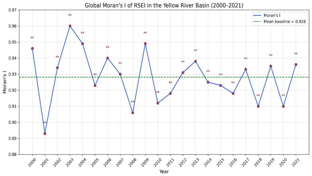
To assess the spatial clustering characteristics of EEQ conditions in the YRB, Global Moran’s I was computed annually for the RSEI from 2000 to 2021. To ascertain the most appropriate spatial analysis scale, Global Moran’s I values were calculated across multiple distance bands (500 m, 1000 m, 1500 m, 2000 m, and 2500 m). All computed results demonstrated statistical significance at the p < 0.01 level, confirming a robust spatial autocorrelation of RSEI values. Notably, the Moran’s I value peaked at 1500 m, suggesting that this distance most effectively captures the underlying spatial structure of EEQ conditions within the study area. Consequently, 1500 m was selected as the optimal spatial lag distance for subsequent spatial autocorrelation and hotspot analyses. As shown in Figure 4, the Global Moran’s I values of RSEI from 2000 to 2021 ranged from 0.893 to 0.96 (mean = 0.93), all significantly positive (p < 0.01), indicating a consistently strong spatial autocorrelation and clustering pattern of EEQ in the YRB. Overall, EEQ exhibited significant positive spatial autocorrelation and a pronounced spatial clustering pattern across the YRB.

3.1.2. RSEI-Based STC Approach Capturing Dynamic Trajectories of Hotspot and Coldspot Evolution

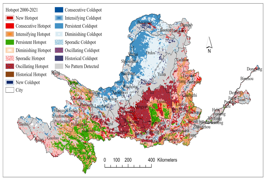
Building on the results of the Global Moran’s I, EHSA was further employed, using an STC method, to identify persistent, intensifying, and diminishing hotspots and coldspots in RSEI values, thereby clarifying the spatial continuity and temporal evolution of EEQ hotspot and coldspot variations across the YRB. By integrating the local spatial statistic Getis–Ord Gi* with the MK trend test, EHSA effectively reveals significant spatiotemporal clustering patterns of EEQ and elucidates which locations are emerging as hotspots or coldspots, as well as whether these trends are intensifying or weakening over time. Based on EHSA of RSEI from 2000 to 2021, 17 distinct spatiotemporal patterns of EEQ hotspots and coldspots were identified across the YRB, revealing marked regional heterogeneity (Figure 5, Table 3). The proportional distribution of these patterns was quantitatively assessed at both the basin scale and within upstream, midstream, and downstream subregions.
From 2000 to 2021, the evolution of EEQ hotspots and coldspots in the YRB exhibited seven major types. Among them, “no pattern detected” accounted for the largest proportion (29.48%), followed by diminishing coldspot (12.97%), oscillating hotspot (11.75%), sporadic hotspot (12.70%), intensifying hotspot (10.97%), persistent hotspot (8.23%), and persistent coldspot (7.52%). These results suggest that areas without significant clustering features accounted for a relatively large proportion of the spatial distribution, while dynamic categories such as diminishing, oscillating, and sporadic hotspots occupied a larger spatial proportion than persistent ones, reflecting the instability and heterogeneity of EEQ changes across the basin.
From 2000 to 2021, the upper reaches of the YRB, functioning as a critical national ecological barrier, exhibited significant improvements in EEQ, although these improvements were spatially constrained. As indicated in Figure 5 and Table 3, areas categorized as intensifying hotspot (8.30%) and persistent hotspot (11.34%) were relatively limited, implying that the ecological benefits from initiatives such as the Sanjiangyuan Ecological Protection Project and grazing exclusion have been substantial but geographically restricted. Notably, the proportion of persistent hotspots in the upper reaches (11.34%) was considerably higher than that in the middle (5.07%) and lower reaches (1.72%), reflecting more stable and sustained EEQ improvements in the upstream region over the past two decades. This pattern can be attributed to both favorable natural conditions, including high elevation and relatively undisturbed ecosystems, and strong institutional protections. However, the occurrence of persistent coldspots (14.12%) and diminishing coldspots (18.03%) indicates sustained ecological stress in alpine grassland areas, likely driven by harsh climatic conditions and the inherently slow recovery capacity of high-altitude ecosystems. Persistent hotspots were predominantly concentrated in the upper reaches of the YRB.
The middle reaches displayed the most complex EEQ dynamics (Figure 5, Table 3). The relatively high proportion of intensifying hotspots (14.47%) reflects localized enhancements in EEQ, while the prevalence of oscillating hotspots (22.63%) highlights frequent fluctuations between EEQ improvement and degradation. However, the existence of diminishing coldspots (8.15%) and persistent coldspots (0.26%) reveals ongoing ecological stress in specific subregions, such as the Loess Plateau. Oscillating hotspots form a circular cluster across Tianshui, Pingliang, Guyuan, Qingyang, Yan’an, and Lüliang in the midstream Loess Plateau. This zone, a core area of the “Three-North Shelterbelt Program,” experiences repeated cycles of degradation and restoration due to intensive land use (e.g., coal mining), urban expansion, and rotational grazing policies, resulting in a characteristic “recovery–degradation–recovery” pattern. In contrast, the middle reaches exhibited a high proportion of oscillating hotspot–coldspot patterns, reflecting strong ecological instability and transitional dynamics. This phenomenon may be associated with the combined influences of intensive soil erosion, ecological restoration activities, land-use conversion, and fluctuating human disturbances in the Loess Plateau region.
In contrast, the lower reaches exhibited a fragmented and less stable EEQ pattern (Figure 5, Table 3). A high proportion of sporadic hotspots (19.57%) and oscillating hotspots (6.34%) reflect irregular and uncertain EEQ changes, likely driven by rapid urban expansion, intensive agriculture, and hydrological interventions. The low occurrence of persistent hotspots (1.72%) indicates limited sustained EEQ improvement. Moreover, the dominance of no pattern detected areas (63.36%) suggests a largely random spatial distribution of EEQ. Overall, the lower reaches were characterized by extensive areas without significant hotspot–coldspot patterns, indicating a relatively fragmented and spatially heterogeneous distribution of EEQ changes.

3.2. Spatiotemporal Dynamics of Key EEQ Hotspot and Coldspot Regions Based on RSEI over Decadal Timescales

3.2.1. Spatiotemporal Transition of EEQ Hotspots and Coldspots for 2000–2010 and 2011–2021

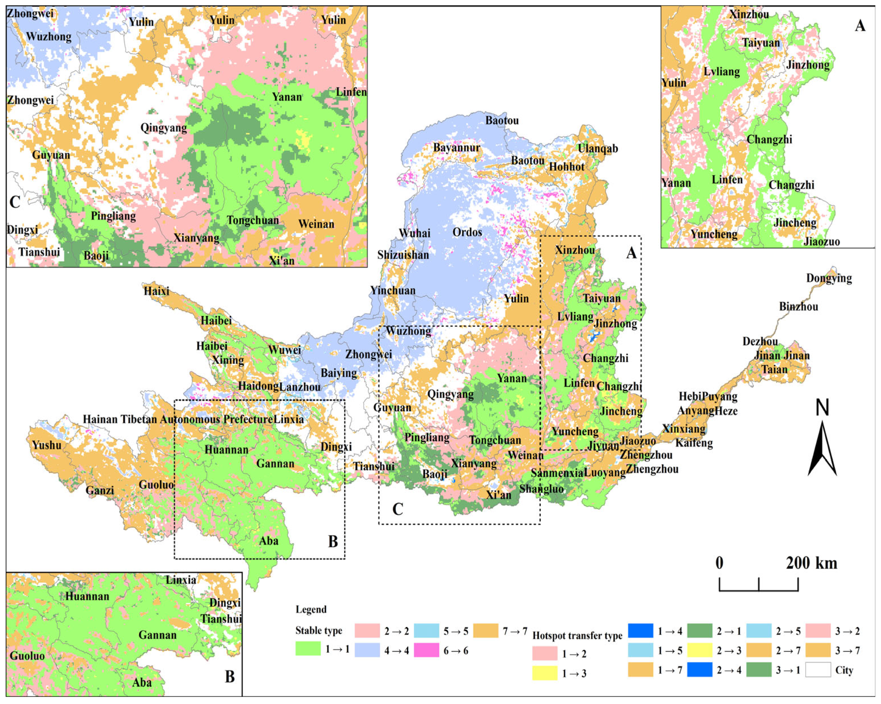
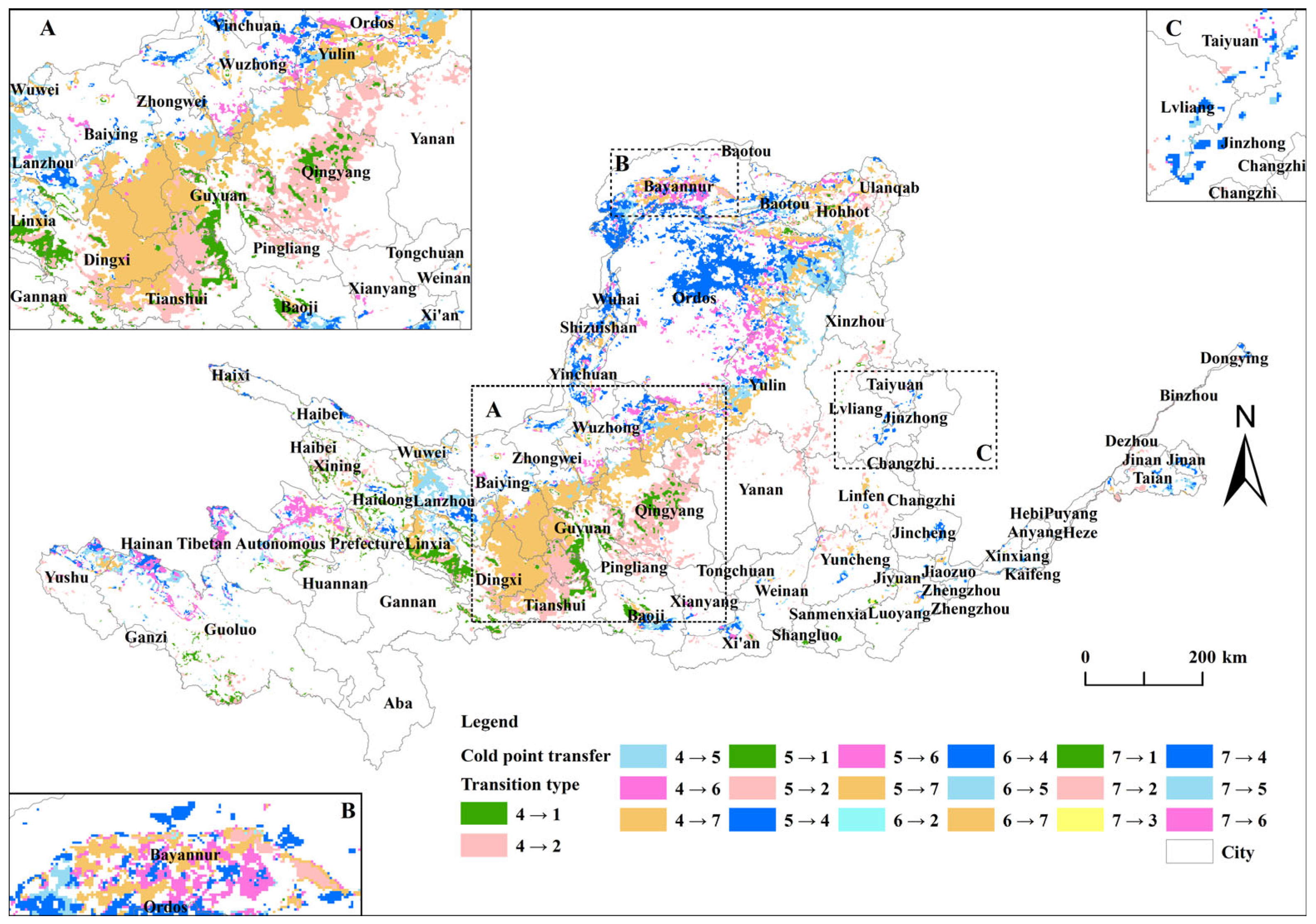
Figure 6 and Figure 7 illustrate the spatiotemporal transitions of EEQ hotspots and coldspots in the YRB across two study periods: 2000–2010 and 2011–2021. To enhance the interpretability of the observed transition patterns, the original 17 EHSA categories were aggregated into seven broader classes that reflect trends in EEQ. These classes include stable hotspot, emerging hotspot, hotspot degradation, stable coldspot, emerging coldspot, coldspot improvement, and no pattern detected (Table 4). This reclassification strategy supports more effective visualization and a more rigorous interpretation of the spatiotemporal dynamics.
As depicted in Figure 6, the spatial distribution of EEQ hotspots and coldspots across the YRB exhibits notable transitions between the two decades. In the upper reaches of the YRB, stable hotspots were primarily distributed across the source region and its adjacent ecological buffer zones, including the Gannan, Huangnan, and Guoluo Tibetan Autonomous Prefectures, as well as parts of the Aba Tibetan and Qiang Autonomous Prefecture (Figure 6B). In the middle reaches of the YRB, particularly around southeastern Yan’an, Tongchuan, and Qingyang, stable hotspot EEQ types are surrounded by a ring of long-term emerging hotspots that have not yet stabilized, reflecting sustained EEQ fluctuation and instability in these transitional zones (Figure 6C). Within the middle reaches of the Yellow River, a north–south-oriented belt of EEQ stable hotspots has formed across Shanxi Province, encompassing the cities of Linfen, Lüliang, Taiyuan, and Xinzhou (Figure 6A). This belt is underpinned by the Lüliang Mountain Ecological Barrier and Fenhe Valley Corridor, which serve as a critical axis for integrating ecological conservation with economic development. This region plays a pivotal role in ecological protection within the YRB and also functions as a strategic pilot zone for Shanxi’s resource-based economic transformation. Along the eastern margin of the middle reaches, stable hotspots are distributed across Jiyuan, Yuncheng, Jincheng, Changzhi, and Jinzhong. In contrast, the northwestern part of the upper reaches, including Baotou, Ordos, Shizuishan, Wuhai, Yinchuan, Wuzhong, Zhongwei, and Baiyin, consistently exhibit the characteristics of a stable coldspot during both periods (Figure 6). This region spans Inner Mongolia, Ningxia, and Gansu, situated within the ecotone between arid and semi-arid zones.
As illustrated in Figure 7, the spatial transitions of EEQ coldspots between the periods 2000–2010 and 2011–2021 across the YRB are evident. A southeast–northwest-oriented transition zone has been identified in the central Loess Plateau, extending across northeastern Pingliang, central Qingyang, and northern Yan’an (Figure 7A). During the period 2000–2010, these regions were identified as EEQ coldspots due to severe soil erosion and vegetation degradation; however, sustained ecological restoration efforts have since transformed them into emerging hotspots. This recovery belt represents the combined effects of natural regeneration and targeted anthropogenic interventions. In contrast, regions such as northeastern Dingxi, southern Baiyin, western Guyuan, southern Zhongwei, northern Qingyang, and western Yulin transitioned from being coldspots to exhibiting no pattern (Figure 7A). The transition of EEQ coldspots in these areas indicates a partial alleviation of ecological environmental stress. In the upper reaches of the YRB, Bayannur serves as a representative example of EEQ coldspot improvement (Figure 7B). Situated at the apex of the Yellow River’s “Great Bend” and constituting the core of the Hetao Irrigation District, this city has exhibited substantial ecological recovery over the past decade. Regions formerly classified as coldspots have largely diminished, transformed into areas with no pattern detected, or even evolved into emerging hotspots, thereby indicating quantifiable enhancements in EEQ. In contrast, a consistently stable coldspot EEQ zone has emerged at the junction of Lüliang, Taiyuan, and Jinzhong (Figure 7C), indicative of prolonged ecological environmental degradation. This region, historically a pivotal coal mining core area in Shanxi Province, serves as a paradigm for the environmental repercussions of resource-dependent development. The persistent clustering of low RSEI values underscores heightened ecological environment stress, thereby emphasizing the significant challenges associated with ecological restoration and sustainable transformation in China’s resource-depleted regions.

3.2.2. Evolutionary Trajectories of EEQ Hotspots and Coldspots Revealed Through Sankey Flow Analysis

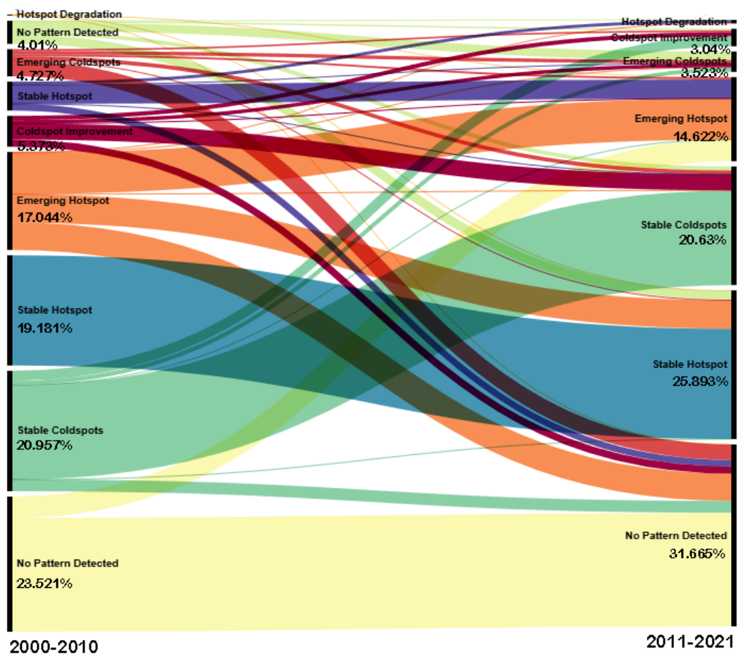
As shown in the Sankey diagram illustrating the transitions of EEQ hotspots and coldspots between the periods 2000–2010 and 2011–2021 (Figure 8), the proportion of areas classified as “No Pattern Detected” increased from 27.53% to 31.67%, reflecting a significant spatial expansion of random ecological environment zones. Specifically, 3.74% of the no pattern detected areas exhibited signs of EEQ improvement and evolved into emerging hotspots, reflecting localized restoration potential. In addition, approximately 4.01% of no pattern detected areas transitioned into stable hotspot, stable coldspot, emerging coldspot, or hotspot degradation areas. The observed transformation dynamics indicate that, despite some regions showing signs of ecological environment recovery, their limited resilience and high sensitivity classify them as “swing zones” or “boundary zones” of EEQ change. Among the total 17.04% of areas identified as emerging hotspots, only 4.94% progressed into stable hotspots, while 7.15% remained in the emerging hotspot category. The remainder transitioned into no pattern detected zones or various coldspot types. Stable coldspot areas accounted for 20.96% and 20.63% of the total study area in 2000–2010 and 2011–2021, respectively, showing negligible change and indicating persistent spatial patterns. Stable hotspots accounted for 24.20% of the study area during the period 2000–2010, increasing slightly to 25.89% in 2011–2021. In contrast, only 1.67% of stable hotspots underwent degradation, either shifting to emerging hotspots or becoming areas with no pattern detected.

3.3. Explaining the Spatiotemporal Heterogeneity of RSEI Drivers Through Integrated Geodetector, OLS, and MGWR Analyses

3.3.1. Attribution Strength and Interactive Effects of RSEI Drivers Based on Geodetector

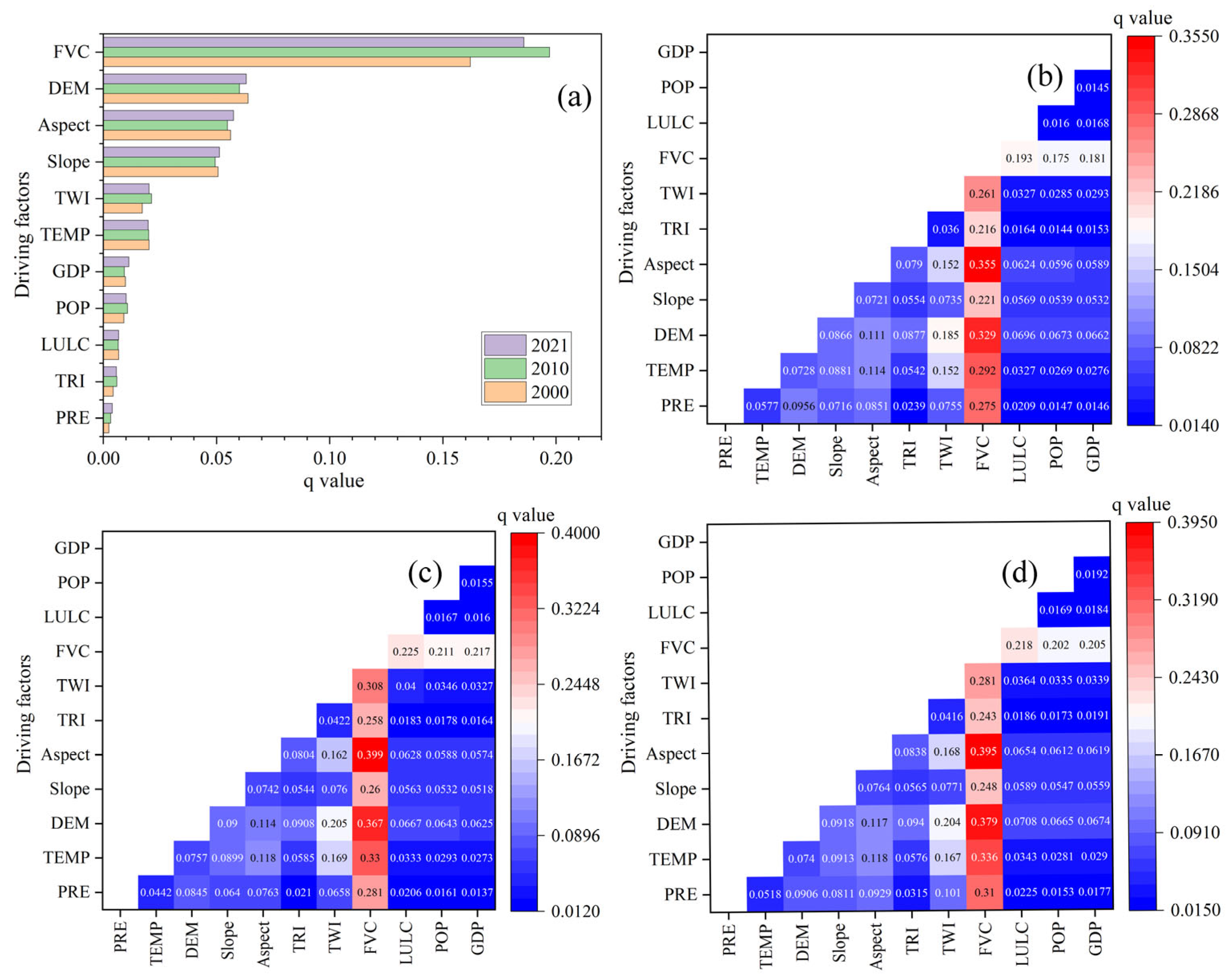
In accordance with the natural and socioeconomic characteristics of the YRB, 11 representative RSEI-related driving factors were incorporated into this study. These included both natural and anthropogenic variables: GDP, POP, LULC, FVC, TRI, TWI, aspect, slope, DEM, TEMP, and PRE. By employing the GD model, the major drivers affecting RSEI in the YRB in the years 2000, 2010, and 2021 were identified, utilizing both univariate and interaction detection methods. All of the drivers demonstrated statistically significant explanatory power for the spatial distribution of RSEI, with p-values less than 0.001. Furthermore, higher q-values suggest a greater explanatory contribution of the respective factor to the spatial variability of RSEI. As shown in Figure 9a, the six primary drivers influencing RSEI variation are FVC, DEM, Aspect, Slope, TWI, and TEMP, highlighting the combined effects of vegetation dynamics and topographic–climatic conditions on EEQ in the YRB. In comparison, socioeconomic and human activity factors, including GDP, POP, LULC, TRI, and PRE, exhibit relatively lower explanatory capacity. As shown in Figure 9b–d, the interaction detection results reveal that, across all three study years (2000, 2010, and 2021), the driving forces of RSEI in the YRB exhibit pronounced enhancement effects through factor interactions. Most combinations of factors display either nonlinear enhancement or bivariate enhancement effects, as evidenced by q ( x 1 x 2 )   >   q ( x 1 )   +   q ( x 2 ) and q ( x 1 x 2 )   >   Max ( q ( x 1 ) , q ( x 2 ) ) . The most significant interaction enhancements were observed between FVC and a range of topographic and climatic factors, including Aspect, Slope, DEM, TEMP, PRE, TWI, TRI, and LULC, with the highest combined q-value reaching 0.40. Moreover, the interactions between LULC and topographic variables such as DEM, Slope, and Aspect evolved from bivariate enhancement in 2000 to nonlinear enhancement by 2021. This transition suggests a growing influence of land use–terrain interactions on EEQ. In contrast, the interaction types of Slope-TRI and LULC-POP changed from nonlinear enhancement in 2000 to bivariate enhancement in 2021, indicating a temporal shift in the interaction patterns among these factors. In summary, natural environmental factors account for the majority of the spatial heterogeneity in the RSEI across the YRB, with FVC exhibiting the strongest explanatory power, while anthropogenic drivers such as ecological restoration policies and socioeconomic development primarily exert their influence through interactions with natural conditions. Notably, the interactions between socioeconomic factors (GDP and POP) and FVC exhibited an increasing trend over time, with the corresponding q-values rising from 0.175 and 0.181 in 2000 to 0.202 and 0.205 in 2021, respectively.

3.3.2. Spatiotemporal Heterogeneity of Key RSEI Drivers Revealed by OLS and MGWR

Based on the GD analysis of 11 natural and anthropogenic variables, FVC, DEM, aspect, slope, TWI, and TEMP were identified as the six most influential drivers of RSEI and were subsequently selected for the MGWR model. PRE, despite its lower individual explanatory power, was also retained due to its strong interactive effects with other variables. To evaluate potential multicollinearity among the selected variables, OLS regression and variance inflation factor (VIF) diagnostics were performed prior to MGWR analysis. According to a VIF threshold of 5, DEM and TEMP were found to exhibit significant collinearity with VIF = 17. However, other topographic variables, including slope, aspect, and TWI, were retained to capture terrain effects. Temperature was subsequently retained for the MGWR to analyze the spatial heterogeneity of RSEI driving mechanisms.
To evaluate the reliability of the MGWR analysis, several diagnostic statistics, including R2, adjusted R2, Akaike Information Criterion corrected (AICc), and residual sum of squares (RSS), were examined (Table 5). The MGWR model exhibited strong explanatory power across all study years, with adjusted R2 values ranging from 0.85 to 0.90, accompanied by relatively low AICc and RSS values.
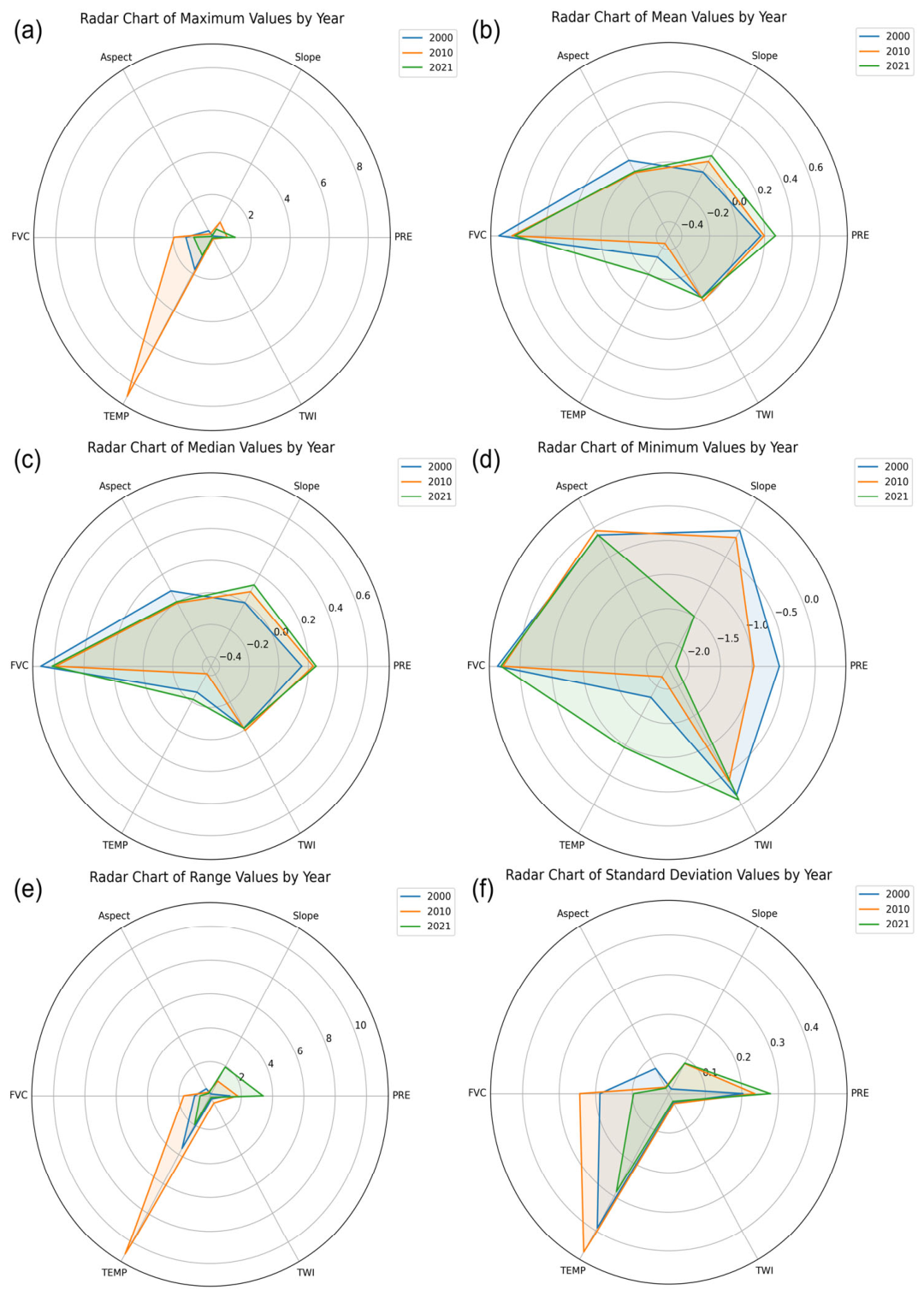
As shown in Figure 10, radar charts visualize the statistical characteristics of MGWR regression coefficients for the six dominant RSEI driving factors in the years 2000, 2010, and 2021. The metrics include maximum, minimum, mean, median, standard deviation, and coefficient range (maximum minus minimum). As shown in Figure 10a,e,f, TEMP in 2010 recorded the highest maximum coefficient (8.70), standard deviation (0.47), and coefficient range (10.86) of the entire study period, revealing substantial spatiotemporal heterogeneity. Coinciding with the extreme climate anomalies in China in 2010, these results suggest that such events can markedly amplify the temperature-EEQ relationship, underscoring the sensitivity of ecosystem quality to temperature variability under extreme conditions. These results highlight TEMP as a “sensitive factor” in 2010 and emphasize the significant impact of abnormal thermal conditions on the spatial variability of RSEI across the YRB. According to the China Climate Bulletin (2010), the year was characterized by an unusually high frequency, intensity, and spatial extent of extreme high-temperature events, phenomena that were rarely recorded in historical data. The national annual mean temperature in 2010 was 0.7 °C above the climatological average, making it the tenth warmest year since 1961 and marking the fourteenth consecutive year with temperatures exceeding the long-term norm. Furthermore, the median, minimum, and mean values of the regression coefficients for FVC are the most distant from the center in the radar plots (Figure 10b–d), indicating that spatial variations in vegetation cover exert a substantial influence on the RSEI across the YRB. In addition, the standard deviations of FVC and PRE coefficients (Figure 10f), second only to that of TEMP, suggest pronounced spatial sensitivity and heterogeneity in their impacts on EEQ. It is noteworthy that the GD results showed relatively stable explanatory power of temperature across the study period, whereas the MGWR results revealed substantially stronger spatial heterogeneity of temperature effects in 2010.
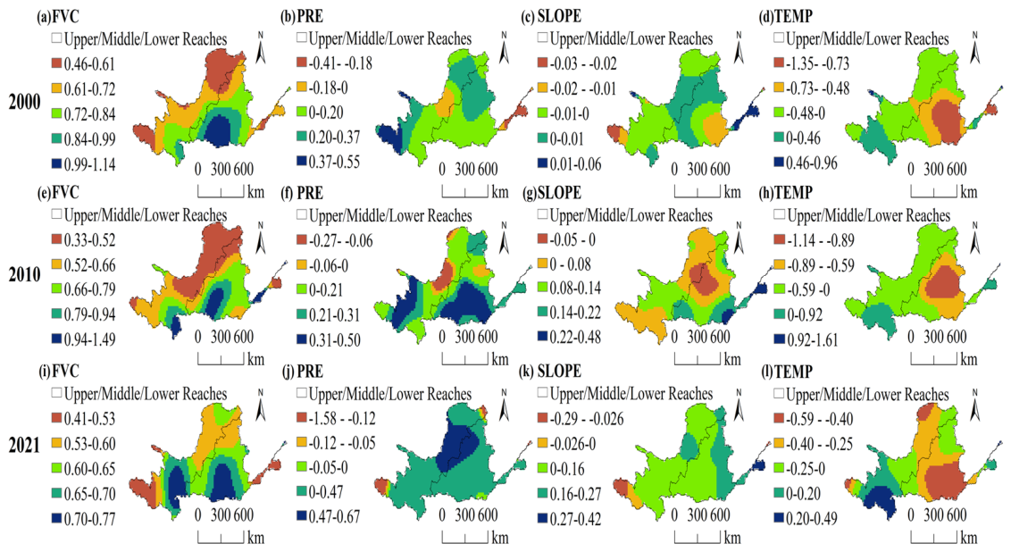
Based on the pronounced spatiotemporal heterogeneity of FVC, TEMP, slope, and PRE effects on RSEI identified, Figure 11 visualizes the standardized MGWR regression coefficients for these factors in 2000, 2010, and 2021, highlighting their spatial patterns and influence strengths across the YRB. The magnitude of factor influences on RSEI varied notably across time, reflecting dynamic shifts in EEQ drivers within the YRB. FVC and TEMP exhibited their strongest effects in 2010, with maximum MGWR coefficients of 1.49 and 1.61, respectively, suggesting heightened vegetation and temperature sensitivity in that year. As shown in Figure 11a,e,i, the regions where FVC exerted the strongest influence on RSEI shifted from the middle reaches in 2010 to the middle and upper reaches in 2021, indicating a spatiotemporal evolution of vegetation-driven effects on EEQ across the YRB. As illustrated in Figure 11b,f,j, precipitation (PRE) exhibited the strongest influence on the RSEI in 2021 compared to other years, with the maximum correlation coefficient reaching 0.67. Regions showing the most pronounced impact were predominantly located in the upstream region of the YRB and along the transitional zone between the midstream and upstream areas.
In terms of directional effects, FVC consistently exerted a positive influence on the RSEI throughout the YRB. Notably, the maximum regression coefficient increased from 1.14 in 2000 to 1.49 in 2010, and subsequently decreased to 0.77 in 2021. As presented in Table 6, the average RSEI across different vegetation coverage categories, including low, moderate, moderately high, and high, was calculated for the years 2000, 2010, and 2021. The results reveal a consistent increase in the mean RSEI values over time within the same vegetation coverage class. Moreover, within each year, areas with higher vegetation coverage exhibit higher mean RSEI values. As shown in Figure 11c,g,k, the negative impact of slope on the RSEI has progressively diminished over time, shifting from a widespread adverse influence in 2000 to a localized negative effect confined to limited areas of the Yellow River source region in 2021. As shown in Figure 11d,h,l, Temp primarily exerted a positive influence on the RSEI in the upstream region of the YRB. The positive temperature–EEQ relationship observed in the upper reaches likely reflects the temperature-limited nature of alpine ecosystems in the source region of the Yellow River [53,54,55]. In these high-altitude environments, moderate warming may alleviate thermal constraints on vegetation growth, prolong the growing season, and enhance ecosystem productivity. As a result, temperature increases can promote ecological improvement rather than ecological stress, leading to positive temperature coefficients in the MGWR results.

3.4. Policy Interventions and Spatiotemporal EEQ Hotspot and Coldspot Responses in the YRB

The spatiotemporal evolution of EEQ hotspots and coldspots in the YRB from 2000 to 2021 closely corresponds to the implementation of major ecological policies (Table 7). From 2000 to 2010, several foundational restoration programs, including the Grain for Green Program (Phase I, initiated in 1999), the Sanjiangyuan Conservation Project (initiated in 2000), and the Check Dam Pilot Project (initiated in 2003), were implemented with the primary objective of reversing severe soil erosion and vegetation degradation. During the first restoration decade (2000–2010), Grain for Green (Phase I) drove extensive Forest and Grassland Restoration (FGR) across the Loess Plateau [56]. These interventions drove rapid vegetation recovery, particularly in the upper and middle reaches, contributing to the emergence of EEQ hotspots across 17.044% of the basin. However, in arid mid-reaches, large-scale afforestation and grassland expansion intensified evapotranspiration, generating water–ecology trade-offs [40,57,58]. This dynamic was reflected in the relatively high proportion of areas without significant spatial clustering (27.531%), indicating that restoration gains were not uniformly stable and underscoring the need for hydrologically balanced intervention strategies.
In contrast, the period from 2011 to 2021 was shaped by systemic governance integration policies, most notably the Revised Yellow River Basin Comprehensive Plan (2012) and Grain for Green Program (Phase II, 2014), as well as targeted poverty-aligned restoration initiatives. These measures emphasized coordinated watershed management, sediment control, and multi-objective ecological protection [59]. These measures consolidated stable hotspots, which increased modestly from 24.20% to 25.89%, with only 4.73% transitioning to other hotspot or coldspot types, suggesting that ecological improvement continued during the second decade, albeit at a slower rate of hotspot expansion. However, the slower expansion of stable hotspots after 2010 should be interpreted cautiously. Given that FVC exhibited the highest explanatory power for EEQ hotspot–coldspot dynamics and is influenced by both ecological restoration activities and climatic variability, the observed EEQ evolution likely reflects the combined influences of anthropogenic interventions and natural environmental processes. Although FVC exhibited the highest explanatory power for EEQ hotspot–coldspot dynamics across all study years, its explanatory contribution was slightly greater in 2010 than in 2021. Given the relatively small magnitude of this difference, the underlying causes remain uncertain based on the current analysis. Restoration saturation effects, climatic anomalies (e.g., extreme drought or temperature events), and their interactions may all have contributed to the observed pattern. Between 2000 and 2021, 24.448% of the entire YRB consisted of sporadic and oscillating hotspots, predominantly distributed in the middle reaches, reflecting spatial instability and ongoing ecological fluctuations (Figure 5, Table 3). The proportion of areas with no significant spatial pattern also rose from 27.53% to 31.67%, highlighting the ecological fragility of these regions and underscoring the need for adaptive, site-specific management strategies (Table 7). This highlights the necessity for adaptive, site-specific restoration approaches that integrate ecological thresholds with socioeconomic conditions, as also emphasized in recent strategic frameworks such as the Yellow River Protection Law (2023). The observed patterns demonstrate that policy evolution, from initial large-scale restoration to integrated and targeted management, has been critical in shaping the spatial distribution and stability of EEQ.
As shown in Table 8, hotspot areas accounted for 46.34%, 44.57%, and 31.68% of the Sanjiangyuan Ecological Conservation Project, Grain for Green Program, and Grazing Withdrawal Program areas, respectively. The relatively high hotspot ratios observed within the Sanjiangyuan and Grain for Green project zones indicate strong spatial correspondence between ecological restoration implementation and long-term EEQ improvement. In contrast, the lower hotspot ratio within the Grazing Withdrawal Program area suggests greater spatial heterogeneity in grassland restoration outcomes.
The observed regional differences in hotspot–coldspot evolution highlight the need for region-specific ecological management. In the upper reaches, maintaining ecosystem stability and climate resilience remains essential. In the middle reaches, restoration strategies should better balance vegetation recovery with water resource availability to mitigate water–ecology trade-offs. In the lower reaches, priority should be given to wetland conservation and ecological connectivity under increasing urbanization pressure. Such targeted strategies may enhance ecological restoration effectiveness and ecological risk management across the Yellow River Basin.

4. Discussion

4.1. Methodological Implications and EEQ Trajectory Detection

In previous studies, RSEI values were often calculated using remote sensing images acquired on similar dates across different years. The selection of years typically followed uniform time intervals, aiming to ensure temporal consistency and comparability. By leveraging the parallel cloud computing capabilities of the GEE platform, this study efficiently calculated annual RSEI values by synthesizing all available remote sensing imagery acquired between July and September from 2000 to 2021. This methodology mitigates potential biases associated with relying on single-date or limited-scene imagery, which may be influenced by extreme weather events or phenological anomalies. Through multi-temporal compositing within the growing season, this approach effectively captures phenological variability across the extensive spatial coverage of the YRB, thereby enhancing the reliability and accuracy of the RSEI assessment [60]. Furthermore, employing a continuous annual time series rather than interval-based observations enables fine-grained tracking of EEQ hotspot–coldspot trajectories, allowing for a more precise characterization of temporal transitions and a deeper understanding of the processes driving ecological improvement and degradation.
Many researchers have employed classical spatial clustering methods, including Getis–Ord Gi* and Local Moran’s I, for assessing the spatial clustering patterns of EEQ at discrete time points [61,62,63]. However, these methods are limited to depicting static spatial distributions of RSEI hotspots and coldspots and are unable to capture the temporal evolution of EEQ hotspot and coldspot patterns. This study represents the first application of an RSEI-driven spatiotemporal analytical approach integrating STC and EHSA to a long-term annual time series of the RSEI in the YRB. By utilizing 22 years (2000–2021) of RSEI time series data and constructing an STC integrated with the MK trend test and Getis–Ord Gi*, we were able to dynamically identify processes including the emergence, persistence, weakening, migration, and disappearance of EEQ coldspots and hotspots within the basin. The diverse transition pathways of EEQ hotspots and coldspots reveal pronounced temporal complexity and spatial heterogeneity across the YRB. In particular, the limited conversion of emerging hotspots into stable hotspots and the relatively modest expansion of stable hotspots suggest that sustained ecological improvement remains challenging, highlighting the importance of adaptive and region-specific restoration strategies. The favorable diagnostic performance of MGWR supports its suitability for examining spatially heterogeneous relationships between EEQ and its driving factors. By allowing explanatory variables to operate at different spatial scales, MGWR provides a more flexible characterization of multiscale and spatially varying driving mechanisms across the YRB. In contrast to traditional methods, the RSEI-based STC method elucidates the critical issue of which locations are emerging as hotspots or coldspots and whether these trends are intensifying or weakening over time. This integration of temporal and spatial dimensions provides a deeper insight into the mechanisms driving EEQ evolution and the underlying influencing factors, thereby enhancing the interpretability of long-term ecosystem dynamics.

4.2. Comparison with Previous Studies and Implications for EEQ Assessment

Previous studies have utilized a variety of comprehensive ecological environment indices to evaluate the EEQ conditions of the YRB. Research conducted by Meiling Zhou et al. [24,41] has shown that the original RSEI model exhibits strong integrative representativeness of EEQ and is particularly suitable for application within the YRB. Due to the basin’s extensive spatial coverage, diverse geomorphological characteristics, complex topography, and climatic variability, identifying universally applicable alternative component indicators across the entire region presents a significant challenge. The pronounced spatial clustering of EEQ indicates strong spatial dependence in ecological conditions across the YRB. Such spatial heterogeneity highlights the importance of considering regional differences when designing ecological restoration and management strategies. The predominance of persistent hotspots in the upper reaches of the YRB may be associated with relatively low anthropogenic disturbance, extensive ecological conservation areas, and the long-term implementation of ecological restoration programs. In addition, the important ecological functions of the upper reaches, including water conservation and grassland protection, may contribute to the stability and continuity of ecological improvement in this region [64]. The prevalence of oscillating hotspot–coldspot patterns in the middle reaches may be associated with the combined influences of intensive soil erosion, ecological restoration activities, land-use conversion, and fluctuating human disturbances in the Loess Plateau region [65]. In contrast, the lower reaches exhibited more fragmented and spatially heterogeneous EEQ patterns, which may be associated with intensive human activities and heterogeneous land-use conditions [66]. The stronger spatial heterogeneity of temperature effects in 2010 suggests that its association with EEQ varied more markedly across space during this period, rather than indicating a uniformly greater explanatory role across the basin. These regional differences highlight the need for region-specific and adaptive ecological restoration strategies.
Furthermore, replacing core RSEI components with alternative indicators may introduce additional uncertainties associated with indicator selection and weighting schemes, which could potentially undermine the model’s consistency and objectivity. Previous evaluations of EEQ in the YRB, conducted by Song Ya-shan (2000–2004) [67] and Dengyu Yin (2000–2010) [68] using comprehensive index-based approaches, consistently revealed an overall improving trend during the period from 2000 to 2010. These findings align with the current study, highlighting that 43.15% of the area experienced measurable improvement over the same period. Tiantian Li et al. reported that EEQ degradation in the YRB intensified progressively from the upstream to the downstream regions during 2000–2019, with the most severe degradation occurring in the downstream provinces of Henan and Shandong [69]. In the lower reaches of the Yellow River, the results of this study show that “no pattern detected” areas dominated, covering 63.36% of the region, while improving hotspots including new, consecutive, intensifying, and persistent hotspots accounted for only 6.41% during the period 2000–2021. Yuqing Tian et al. found that regions exhibiting degraded ecological environment conditions are predominantly located in the northern part of the YRB, a finding that aligns well with the results of the present study [70].
Beyond RSEI-based assessments, other remote sensing-derived composite indicators provide complementary perspectives for understanding ecosystem dynamics. For example, Dynamic Habitat Indices (DHIs) incorporate temporal vegetation dynamics and environmental variability, offering additional information on habitat changes and ecosystem responses to climatic fluctuation [26,71]. Vegetation-based indicators, such as NDVI and EVI, are effective for characterizing vegetation productivity and phenological changes, whereas NPP-based indices provide insights into ecosystem carbon assimilation and productivity [72,73]. However, these indicators generally emphasize specific ecological functions or processes rather than overall ecosystem condition. Therefore, RSEI remains particularly suitable for this study because the primary objective is to identify long-term EEQ evolution trajectories and hotspot–coldspot transition patterns by integrating multiple ecological dimensions. Nevertheless, integrating RSEI with complementary indicators, such as habitat dynamics, ecosystem productivity, climate extremes, and land-surface changes, may further improve future ecological monitoring frameworks by providing a more comprehensive understanding of ecosystem conditions, functions, and responses under complex environmental pressures.

4.3. Implications Beyond the YRB

Compared with other major river basins, such as the Mekong and Amazon basins, the YRB is characterized by the combined influences of pronounced climatic gradients, intensive ecological restoration, and rapid socioeconomic transformation [74,75]. The EEQ evolution in the basin reflects complex interactions among ecological engineering, climate variability, land use changes, and human activities, resulting in diverse hotspot–coldspot transition patterns. While previous studies have primarily focused on EEQ assessment and overall trend evaluation [24,76], the process-oriented STC–EHSA–GD–MGWR framework developed in this study enables the identification of ecological persistence, transition trajectories, and spatially heterogeneous driving mechanisms. Many large river basins worldwide face similar challenges related to climate variability, land degradation, ecological restoration, and human pressures. Therefore, this framework provides a potentially transferable perspective for exploring long-term ecological dynamics in other large and heterogeneous river basins, where identifying ecological trajectories and their driving mechanisms is essential for adaptive ecosystem management.

4.4. Limitations and Future Research Directions

The EHSA based on the RSEI identified 17 types of EEQ hotspots and coldspots, reflecting the complex temporal dynamics of EEQ in the YRB. This classification offers valuable insights into spatiotemporal change patterns and supports region-specific policy design. For transition analysis between the periods 2000–2010 and 2011–2021, the 17 categories were streamlined into seven broader typologies to improve computational efficiency. While this streamlining improved analytical tractability and preserved major spatiotemporal distinctions, it inevitably limited the capacity to detect more subtle ecological dynamics. In addition, RSEI does not explicitly account for ecological dimensions such as biodiversity, soil pollution, or ecosystem services [27]. Furthermore, MGWR results may be influenced by bandwidth optimization and parameter selection. Future work should therefore adopt refined algorithms and statistical techniques to capture nuanced EEQ trajectories with greater precision.
Beyond methodological refinement, future studies should extend toward policy and governance perspectives. Integrated models are needed to link phased ecological policies with EEQ dynamics, incorporating hydrological, climatic, and socioeconomic factors to better anticipate trade-offs between vegetation restoration and water availability [77]. Assessing how restoration aligns with local livelihoods and SDG objectives, while conducting cross-basin comparisons, will help identify generalizable drivers and effective governance pathways [78]. Future work could extend this process-oriented analytical framework to other ecological systems, enabling comparative analyses of spatiotemporal evolution patterns and enhancing the predictive modeling of ecological resilience.

5. Conclusions

This study developed a process-oriented RSEI space–time cube framework on the GEE to characterize long-term EEQ dynamics in the YRB. By integrating EHSA with GD, OLS, and MGWR, the approach provides a unified framework for detecting hotspot–coldspot evolution trajectories and identifying their multiscale drivers. The main conclusions are as follows:
(1) The RSEI-based space–time cube successfully identified 17 hotspot–coldspot evolution patterns and revealed their temporal persistence, emergence, oscillation, and decay. This process-oriented classification advances beyond static EEQ assessments and captures cumulative temporal effects associated with ecological improvement and degradation.
(2) Significant transitions occurred between 2000 and 2010, and 2011 and2021, including stable hotspot cores, coldspot conversion zones, and widespread oscillating patterns characterized by recovery–degradation–recovery cycles. These transitions highlight substantial ecological instability and identify key areas requiring priority management.
(3) Spatial heterogeneity of EEQ was pronounced across the basin. Persistent hotspots were concentrated in the upper reaches, while intensifying, oscillating, and sporadic hotspots dominated the middle reaches. The lower reaches experienced accelerating degradation, underscoring the need for targeted interventions in ecologically vulnerable zones.
(4) MGWR revealed strong spatiotemporal heterogeneity in driving forces, with temperature exerting amplified effects during periods of climatic anomalies. This demonstrates the increasing sensitivity of the basin to climate variability.
(5) FVC exhibited the highest explanatory power of EEQ evolution, followed by topography and temperature. FVC generally enhanced EEQ, whereas slope effects weakened over time. The interplay between natural factors and human activities shaped the spatial clustering of hotspots and coldspots, highlighting the basin’s ecological fragility.
Scientifically, this study advances conventional status- and trend-oriented EEQ assessments toward a process-oriented perspective by integrating hotspot–coldspot persistence, transition trajectories, and spatially heterogeneous driving mechanisms within a unified analytical framework. The proposed framework provides a potentially transferable approach for investigating long-term ecological trajectories in other large and environmentally heterogeneous river basins. Practically, the identification of persistent, transitional, and unstable ecological trajectories provides spatially explicit evidence for differentiated ecological restoration strategies, ecological risk identification, and adaptive basin management.

Supplementary Materials

The following supporting information can be downloaded at: https://www.mdpi.com/article/10.3390/land15081379/s1. Figure S1: RSEI values in the Yellow River Basin from 2000 to 2021. Table S1: RSEI composition indicators and associated formulas. Table S2: Principal component analysis results. Table S3: Reclassification scheme of EHSA based on EEQ change trends based on ArcGIS Pro 3.3.1.

Author Contributions

Conceptualization, Z.H.; methodology, Z.H. and Z.Z.; software, Z.H. and S.L.; validation, Z.Z. and Q.G.; formal analysis, Z.W. and X.L.; investigation, X.L. and Z.H.; resources, Z.H. and Q.G.; data curation, Z.H. and Q.G.; writing—original draft preparation, Z.H.; writing—review and editing, Z.H.; visualization, Z.H. and S.L.; supervision, Z.W.; project administration, Q.G.; funding acquisition, Q.G. and X.L. All authors have read and agreed to the published version of the manuscript.

Funding

This research was supported by Shandong Provincial Natural Science Foundation (Grant No. ZR2023MD075) and the National Natural Science Foundation of China (NSFC) Joint Fund for Earth Sciences (Grant No. U2444217).

Data Availability Statement

The data presented in this study are publicly available from the National Cryosphere Desert Data Center (https://www.ncdc.ac.cn/portal/) (accessed on 21 May 2026) at https://doi.org/10.12072/ncdc.nieer.db6977.2025.

Acknowledgments

The authors are thankful for the data support from the National Earth System Science Data Center, National Science & Technology Infrastructure of China (http://www.geodata.cn). The authors express sincere gratitude to all departments that contributed data for this study. Particular thanks are given to the anonymous reviewers and editors for their valuable and insightful comments, which have greatly strengthened the manuscript.

Conflicts of Interest

The authors declare no conflict of interest.

References

  1. Nicholson, E.; Keith, D.A.; Wilcove, D.S. Assessing the Threat Status of Ecological Communities. Conserv. Biol. 2009, 23, 259–274. [Google Scholar] [CrossRef] [PubMed]
  2. Mackay, S.; Hales, R.; Hewson, J.; Addis, R.; Mackey, B. Addressing climate inaction as our greatest threat to sustainable development. Glob. Environ. Change 2025, 91, 102969. [Google Scholar] [CrossRef]
  3. Wei, W.; Zhang, Y.; Wei, X.; Xie, B.; Ma, Z.; Liu, C.; Yu, L.; Zhou, J.; Shi, W.; Liu, T.; et al. Construction and optimization of ecological security patterns based on ecosystem service function and ecosystem sensitivity in the important ecological functional area—A case study in the Yellow River Basin. Ecol. Eng. 2025, 215, 107609. [Google Scholar] [CrossRef]
  4. Zhao, L.; Chen, M.-n.; Yang, C.-h.; Zhang, R.-z.; Zhang, Q.-p.; Wang, Q. Characteristics of spatial and temporal carbon emissions from different land uses in Shanxi section of the Yellow River, China. Environ. Dev. Sustain. 2024, 26, 20869–20884. [Google Scholar] [CrossRef]
  5. Wohlfart, C.; Kuenzer, C.; Chen, C.; Liu, G. Social–ecological challenges in the Yellow River basin (China): A review. Environ. Earth Sci. 2016, 75, 1066. [Google Scholar] [CrossRef]
  6. Xu, H.; Wang, Y.; Guan, H.; Shi, T.; Hu, X. Detecting Ecological Changes with a Remote Sensing Based Ecological Index (RSEI) Produced Time Series and Change Vector Analysis. Remote Sens. 2019, 11, 2345. [Google Scholar] [CrossRef]
  7. Yang, Z.; Tian, J.; Su, W.; Wu, J.; Liu, J.; Liu, W.; Guo, R. Analysis of ecological environmental quality change in the Yellow River Basin using the remote-sensing-based ecological index. Sustainability 2022, 14, 10726. [Google Scholar] [CrossRef]
  8. Chen, F.; Huang, H.; Yang, G.; Li, X. Research on the dynamic change of the ecological environment and its influencing factors in the Yellow River basin based on Remote Sensing Ecological Index. J. Desert Res. 2023, 43, 252–262. [Google Scholar]
  9. Xu, Y.; Yang, X.; Xing, X.; Wei, L. Coupling eco-environmental quality and ecosystem services to delineate priority ecological reserves—A case study in the Yellow River Basin. J. Environ. Manag. 2024, 365, 121645. [Google Scholar] [CrossRef] [PubMed]
  10. Wang, F.; Li, W.-H.; Lin, Y.-M.; Nan, X.-X.; Hu, Z.-R. Spatiotemporal pattern and driving force analysis of ecological environmental quality in typical ecological areas of the Yellow River Basin from 1990 to 2020. Huan Jing Ke Xue = Huanjing Kexue 2023, 44, 2518–2527. [Google Scholar] [PubMed]
  11. Liu, J.; Hu, Y.; Feng, Z.; Xiao, C. A Review of Land Use and Land Cover in Mainland Southeast Asia over Three Decades (1990–2023). Land 2025, 14, 828. [Google Scholar] [CrossRef]
  12. Liu, X.; Ruibo, C.; Lijuan, H.; Rundong, L.; Shuhong, M.; Chanling, P.; Jiaxing, C.; Zhou, G. Ecological quality assessment of large-scale regions using RSEI improved with YTT temperature rectification. Int. J. Remote Sens. 2025, 46, 4274–4294. [Google Scholar] [CrossRef]
  13. Zhen, B.; Dang, G.; Zhu, L. Spatio-temporal changes and driving forces of ecological environment quality in northern China from 2000 to 2022. J. Geogr. Sci. 2025, 35, 763–782. [Google Scholar] [CrossRef]
  14. Boori, M.S.; Choudhary, K.; Paringer, R.; Kupriyanov, A. Spatiotemporal ecological vulnerability analysis with statistical correlation based on satellite remote sensing in Samara, Russia. J. Environ. Manag. 2021, 285, 112138. [Google Scholar] [CrossRef] [PubMed]
  15. Hägerstrand, T. What about people in regional science. Pap. Reg. Sci. 1970, 24, 7–21. [Google Scholar] [CrossRef]
  16. Ogungbire, A.; Pulugurtha, S.S. Spatiotemporal Risk Mapping of Statewide Weather-related Traffic Crashes: A Machine Learning Approach. Mach. Learn. Appl. 2025, 20, 100642. [Google Scholar] [CrossRef]
  17. Wei, J.; Zhong, Y.; Chen, A.; Tang, H.; Li, D. Space-time cube reveals escalating light pollution in China’s national parks: Impact of boundary geometry and human activities (1992–2021). Environ. Pollut. 2025, 377, 126462. [Google Scholar] [CrossRef] [PubMed]
  18. Cao, Z.; Wu, M.; Wang, D.; Wan, B.; Jiang, H.; Tan, X.; Zhang, Q. Space-time cube uncovers spatiotemporal patterns of basin ecological quality and their relationship with water eutrophication. Sci. Total Environ. 2024, 916, 170195. [Google Scholar] [CrossRef] [PubMed]
  19. Feng, Y.; Huang, D.; Hong, X.; Wang, H.; Loughney, S.; Wang, J. Spatial-Temporal Evolution of Maritime Accident Hot Spots in the East China Sea: A Space-Time Cube Representation. J. Mar. Sci. Eng. 2025, 13, 233. [Google Scholar] [CrossRef]
  20. Kovacs-Györi, A.; Lahnsteiner, D.; Schmitt, J.; Prinz, T. Spatiotemporal clustering based on international tourists’ overnight stay data in Salzburg, Austria: A seasonal analysis using space-time data cubes to enhance airport connectivity. Tour. Recreat. Res. 2025, 50, 1806–1825. [Google Scholar] [CrossRef]
  21. Wang, Z.; Yu, Y.; Cheng, Y.; Liu, D.; Cheng, Y.; Pereira, P. Land use and RSEI spatial-temporal changes in Horqin Sandland (Inner Mongolia, China). Ecol. Front. 2025, 45, 849–861. [Google Scholar] [CrossRef]
  22. Kamara, D.M.; Yang, Z.; Lahai, Y.A. Ecological Geospatial Monitoring and Assessment of Surface Water Environment Using Remote Sensing Ecological Index Model (RSEI) in Freetown, Sierra Leone, from 2010 to 2018. GSJ 2020, 8, 328–348. [Google Scholar]
  23. Karbalaei Saleh, S.; Amoushahi, S.; Gholipour, M. Spatiotemporal ecological quality assessment of metropolitan cities: A case study of central Iran. Environ. Monit. Assess. 2021, 193, 305. [Google Scholar] [CrossRef] [PubMed]
  24. Zhou, M.; Li, Z.; Gao, M.; Zhu, W.; Zhang, S.; Ma, J.; Ta, L.; Yang, G. Revealing the Eco-Environmental Quality of the Yellow River Basin: Trends and Drivers. Remote Sens. 2024, 16, 2018. [Google Scholar] [CrossRef]
  25. Wang, P.; Cheng, J.; Ma, S.; Yang, J.; Sun, H.; Zhao, J. Divergent Greenness and Productivity Recovery Potentials Across China’s Eight Forestry Engineering Regions During 2001–2025. Forests 2026, 17, 813. [Google Scholar] [CrossRef]
  26. Radeloff, V.C.; Dubinin, M.; Coops, N.C.; Allen, A.M.; Brooks, T.M.; Clayton, M.K.; Costa, G.C.; Graham, C.H.; Helmers, D.P.; Ives, A.R. The Dynamic Habitat Indices (DHIs) from MODIS and global biodiversity. Remote Sens. Environ. 2019, 222, 204–214. [Google Scholar] [CrossRef]
  27. Safaei, M.; Kleinebecker, T.; Weis, M.; Große-Stoltenberg, A. Tracking effects of extreme drought on coniferous forests from space using dynamic habitat indices. Heliyon 2024, 10, e27864. [Google Scholar] [CrossRef] [PubMed]
  28. Haque, M.R.; Moniruzzaman, M.; Arman; Hasan, M.R.; Lat, T.; Kabir, N.; Sarker, M.J.; Tijing, L.; Shon, H.K.; Ayejoto, D.A.; et al. Land use Transition and Ecological Consequences: A Spatiotemporal Analysis in South-Eastern Bangladesh. Earth Syst. Environ. 2025, 9, 1135–1148. [Google Scholar] [CrossRef]
  29. Wang, J.; Xu, C. Geodetector: Principle and prospective. Acta Geogr. Sin. 2017, 72, 116–134. [Google Scholar] [CrossRef]
  30. He, Z.; Guo, Q.; Yin, Z.; Luo, X.; Sun, M. Evolution and driving mechanisms of eco-environmental quality across different urbanization stages. Sci. Rep. 2025, 15, 22101. [Google Scholar] [CrossRef] [PubMed]
  31. Chen, A.; Yang, X.; Guo, J.; Zhang, M.; Xing, X.; Yang, D.; Xu, B.; Jiang, L. Dynamic of land use, landscape, and their impact on ecological quality in the northern sand-prevention belt of China. J. Environ. Manag. 2022, 317, 115351. [Google Scholar] [CrossRef] [PubMed]
  32. Xia, J.; Zhang, G.; Ma, S.; Pan, Y. Spatial Heterogeneity of Driving Factors in Multi-Vegetation Indices RSEI Based on the XGBoost-SHAP Model: A Case Study of the Jinsha River Basin, Yunnan. Land 2025, 14, 925. [Google Scholar] [CrossRef]
  33. Wu, N.; Zhou, Y.; Yin, S.; Gong, H.; Zhang, C. Revealing the nonlinear impact of environmental regulation on ecological resilience using the XGBoost-SHAP model: Evidence from the Yangtze River Delta region, China. J. Clean. Prod. 2025, 514, 145700. [Google Scholar] [CrossRef]
  34. Guo, Q.; He, Z.; Wang, Z. Prediction of monthly average and extreme atmospheric temperatures in Zhengzhou based on artificial neural network and deep learning models. Front. For. Glob. Change 2023, 6, 1249300. [Google Scholar] [CrossRef]
  35. Guo, Q.; He, Z.; Wang, Z. The Characteristics of Air Quality Changes in Hohhot City in China and their Relationship with Meteorological and Socio-economic Factors. Aerosol Air Qual. Res. 2024, 24, 230274. [Google Scholar] [CrossRef]
  36. Liu, W.; Cheng, Z.; Li, J.; Li, G.; Pan, N. Assessment of ecological asset quality and its drivers in Agro-pastoral Ecotone of China. Ecol. Indic. 2025, 170, 113072. [Google Scholar] [CrossRef]
  37. Zeng, J.; Luo, T.; Gu, T.; Chen, W. How does cultivated land fragmentation affect soil erosion: Evidence from the Yangtze River Basin in China. J. Environ. Manag. 2024, 360, 121020. [Google Scholar] [CrossRef] [PubMed]
  38. Li, J.; Sun, W.; Li, M.; Linlin, M. Coupling coordination degree of production, living and ecological spaces and its influencing factors in the Yellow River Basin. J. Clean. Prod. 2021, 298, 126803. [Google Scholar] [CrossRef]
  39. Yang, H.; Yu, J.; Xu, W.; Wu, Y.; Lei, X.; Ye, J.; Geng, J.; Ding, Z. Long-time series ecological environment quality monitoring and cause analysis in the Dianchi Lake Basin, China. Ecol. Indic. 2023, 148, 110084. [Google Scholar] [CrossRef]
  40. Feng, X.; Fu, B.; Piao, S.; Wang, S.; Ciais, P.; Zeng, Z.; Lü, Y.; Zeng, Y.; Li, Y.; Jiang, X.; et al. Revegetation in China’s Loess Plateau is approaching sustainable water resource limits. Nat. Clim. Change 2016, 6, 1019–1022. [Google Scholar] [CrossRef]
  41. Li, W.; Wang, W.; Chen, J.; Zhang, Z. Assessing effects of the Returning Farmland to Forest Program on vegetation cover changes at multiple spatial scales: The case of northwest Yunnan, China. J. Environ. Manag. 2022, 304, 114303. [Google Scholar] [CrossRef] [PubMed]
  42. Yang, F.; He, F.; Wang, Y.; Zhou, S.; Dong, G. Reconstructing forest cover changes for the middle and lower reaches of the Yellow River over the past millennium. Reg. Environ. Change 2024, 24, 18. [Google Scholar] [CrossRef]
  43. Du, L.; Dong, C.; Kang, X.; Qian, X.; Gu, L. Spatiotemporal evolution of land cover changes and landscape ecological risk assessment in the Yellow River Basin, 2015–2020. J. Environ. Manag. 2023, 332, 117149. [Google Scholar] [CrossRef] [PubMed]
  44. Cheng, C.; Wang, Y. Spatiotemporal Changes and the Drivers of Ecological Environmental Quality Based on the Remote Sensing Ecological Index: A Case Study of Shanxi Province, China. Land 2025, 14, 952. [Google Scholar] [CrossRef]
  45. Shao, Q.; Liu, S.; Ning, J.; Liu, G.; Yang, F.; Zhang, X.; Niu, L.; Huang, H.; Fan, J.; Liu, J. Assessment of ecological benefits of key national ecological projects in China in 2000-2019 using remote sensing. Acta Geogr. Sin. 2022, 77, 2133–2153. [Google Scholar] [CrossRef]
  46. Xu, H. A remote sensing index for assessment of regional ecological changes. China Environ. Sci. 2013, 33, 889–897. [Google Scholar]
  47. Moran, P.A. Notes on continuous stochastic phenomena. Biometrika 1950, 37, 17–23. [Google Scholar] [CrossRef]
  48. Wooldridge, J.M. Econometric Analysis of Cross Section and Panel Data; MIT Press: Cambridge, MA, USA, 2010. [Google Scholar]
  49. Wang, J.-F.; Zhang, T.-L.; Fu, B.-J. A measure of spatial stratified heterogeneity. Ecol. Indic. 2016, 67, 250–256. [Google Scholar] [CrossRef]
  50. Fotheringham, A.S.; Yang, W.; Kang, W. Multiscale geographically weighted regression (MGWR). Ann. Am. Assoc. Geogr. 2017, 107, 1247–1265. [Google Scholar] [CrossRef]
  51. Getis, A.; Ord, J.K. The Analysis of Spatial Association by Use of Distance Statistics. Geogr. Anal. 1992, 24, 189–206. [Google Scholar] [CrossRef]
  52. LaDue, C.A.; Farinelli, S.M.; Eranda, I.; Jayasinghe, C.; Vandercone, R.P. The influence of habitat changes on elephant mortality associated with human–elephant conflict: Identifying areas of concern in the north central dry zone of Sri Lanka. Sustainability 2021, 13, 13707. [Google Scholar] [CrossRef]
  53. Jin, A.; Li, H.; Wang, X.; Wang, Z. Spatiotemporal assessment of ecological quality and driving mechanisms in the Beijing metropolitan area. Sci. Rep. 2025, 15, 13136. [Google Scholar] [CrossRef] [PubMed]
  54. Li, X.; Jiang, L.; Meng, F.; Wang, S.; Niu, H.; Iler, A.M.; Duan, J.; Zhang, Z.; Luo, C.; Cui, S.; et al. Responses of sequential and hierarchical phenological events to warming and cooling in alpine meadows. Nat. Commun. 2016, 7, 12489. [Google Scholar] [CrossRef] [PubMed]
  55. Guo, L.; Chen, J.; Luedeling, E.; He, J.-S.; Cheng, J.; Wen, Z.; Peng, C. Early-spring soil warming partially offsets the enhancement of alpine grassland aboveground productivity induced by warmer growing seasons on the Qinghai-Tibetan Plateau. Plant Soil 2018, 425, 177–188. [Google Scholar] [CrossRef]
  56. Yang, J.; Huang, X. The 30 m annual land cover dataset and its dynamics in China from 1990 to 2019. Earth Syst. Sci. Data 2021, 13, 3907–3925. [Google Scholar] [CrossRef]
  57. Cao, M.; Wang, W.; Wei, J.; Forzieri, G.; Fetzer, I.; Wang-Erlandsson, L. Revegetation impacts on moisture recycling and precipitation trends in the Chinese Loess Plateau. Water Resour. Res. 2024, 60, e2024WR038199. [Google Scholar] [CrossRef]
  58. Chen, Y.; Wang, K.; Lin, Y.; Shi, W.; Song, Y.; He, X. Balancing green and grain trade. Nat. Geosci. 2015, 8, 739–741. [Google Scholar] [CrossRef]
  59. Yibin, W.; Fei, L.; Jian, W.; Hongyu, C.; Mengfei, L. The social-ecological benefits of grain for green program based on coupled coordination network: Taking the China’s Loess Plateau as an example. Land Use Policy 2024, 143, 107211. [Google Scholar] [CrossRef]
  60. Yang, X.; Meng, F.; Fu, P.; Wang, Y.; Liu, Y. Time-frequency optimization of RSEI: A case study of Yangtze River Basin. Ecol. Indic. 2022, 141, 109080. [Google Scholar] [CrossRef]
  61. He, Y.; Ye, B.; He, J.; Wang, H.; Zhou, W. Long Time-Series Monitoring and Drivers of Eco-Quality in the Upper-Middle Fen River Basin of the Eastern Loess Plateau: An Analysis Based on a Remote Sensing Ecological Index and Google Earth Engine. Land 2024, 13, 2239. [Google Scholar] [CrossRef]
  62. Wu, T.; Zhou, L.; Jiang, G.; Meadows, M.E.; Zhang, J.; Pu, L.; Wu, C.; Xie, X. Modelling Spatial Heterogeneity in the Effects of Natural and Socioeconomic Factors, and Their Interactions, on Atmospheric PM2.5 Concentrations in China from 2000–2015. Remote Sens. 2021, 13, 2152. [Google Scholar] [CrossRef]
  63. Wang, X.; Shi, S.; Zhao, X.; Hu, Z.; Hou, M.; Xu, L. Detecting Spatially Non-Stationary between Vegetation and Related Factors in the Yellow River Basin from 1986 to 2021 Using Multiscale Geographically Weighted Regression Based on Landsat. Remote Sens. 2022, 14, 6276. [Google Scholar] [CrossRef]
  64. Li, X.; Yu, K.; Xu, G.; Li, P.; Li, Z.; Shi, P.; Jia, L. Exploring ecosystem service dynamics and drivers in the upper and middle Yellow River Basin under large-scale ecological restoration. Ecol. Eng. 2025, 217, 107643. [Google Scholar] [CrossRef]
  65. Bai, R.; Wang, X.; Li, J.; Yang, F.; Shangguan, Z.; Deng, L. The impact of vegetation reconstruction on soil erosion in the Loess plateau. J. Environ. Manag. 2024, 363, 121382. [Google Scholar] [CrossRef] [PubMed]
  66. Yu, G.; Liu, T.; Wang, Q.; Li, T.; Li, X.; Song, G.; Feng, Y. Impact of land use/land cover change on ecological quality during urbanization in the lower Yellow River Basin: A case study of Jinan City. Remote Sens. 2022, 14, 6273. [Google Scholar] [CrossRef]
  67. Ya-shan, S.; Chong, D.; Chao, Y.; Chao, Q. Ecological Environmental Quality Evaluation of Yellow River Basin. Procedia Eng. 2012, 28, 754–758. [Google Scholar] [CrossRef][Green Version]
  68. Yin, D.; Li, X.; Li, G.; Zhang, J.; Yu, H. Spatio-Temporal Evolution of Land Use Transition and Its Eco-Environmental Effects: A Case Study of the Yellow River Basin, China. Land 2020, 9, 514. [Google Scholar] [CrossRef]
  69. Li, T.; Zhang, Q.; Singh, V.P.; Zhao, J.; Song, J.; Sun, S.; Wang, G.; Shen, Z.; Wu, W. Identification of Degradation Areas of Ecological Environment and Degradation Intensity Assessment in the Yellow River Basin. Front. Earth Sci. 2022, 10, 922013. [Google Scholar] [CrossRef]
  70. Tian, Y.; Wen, Z.; Zhang, X.; Cheng, M.; Xu, M. Exploring a multisource-data framework for assessing ecological environment conditions in the Yellow River Basin, China. Sci. Total Environ. 2022, 848, 157730. [Google Scholar] [CrossRef] [PubMed]
  71. Hobi, M.L.; Dubinin, M.; Graham, C.H.; Coops, N.C.; Clayton, M.K.; Pidgeon, A.M.; Radeloff, V.C. A comparison of Dynamic Habitat Indices derived from different MODIS products as predictors of avian species richness. Remote Sens. Environ. 2017, 195, 142–152. [Google Scholar] [CrossRef]
  72. Song, K.; Knighton, J.; Qiu, S.; Yang, X.; Suh, J.W.; Tavares, J.V.; Liu, Y.; Tai, X.; Fahey, R.; Neigh, C.S.R.; et al. Physiological fidelity of a satellite-derived forest resilience indicator in the Amazon. Nat. Ecol. Evol. 2026. [Google Scholar] [CrossRef] [PubMed]
  73. Hu, X.; Feng, H.; Tang, Y.; Wang, S.; Wang, S.; Wang, W.; Huang, J. Detection of the contribution of vegetation change to global net primary productivity: A satellite perspective. Remote Sens. 2024, 16, 4692. [Google Scholar] [CrossRef]
  74. Gatti, L.V.; Basso, L.S.; Miller, J.B.; Gloor, M.; Gatti Domingues, L.; Cassol, H.L.G.; Tejada, G.; Aragão, L.E.O.C.; Nobre, C.; Peters, W.; et al. Amazonia as a carbon source linked to deforestation and climate change. Nature 2021, 595, 388–393. [Google Scholar] [CrossRef] [PubMed]
  75. Kummu, M.; Varis, O. Sediment-related impacts due to upstream reservoir trapping, the Lower Mekong River. Geomorphology 2007, 85, 275–293. [Google Scholar] [CrossRef]
  76. Li, G.; Zhang, N.; Cao, Y.; Xia, Z.; Bao, C.; Fan, L.; Xue, S. Analysis of the temporal and spatial changes of ecological environment quality using the optimization remote sensing ecological index in the middle Yellow River Basin, China. Earth Sci. Inform. 2024, 17, 5107–5122. [Google Scholar] [CrossRef]
  77. Ge, L.; Mei, X.; Ping, J.; Liu, E.; Xie, J.; Feng, J. Identification of suitable vegetation restoration areas and carrying capacity thresholds on the Loess Plateau. J. Environ. Manag. 2025, 373, 123660. [Google Scholar] [CrossRef] [PubMed]
  78. Yin, C.; Zhao, W.; Pereira, P. Ecosystem restoration along the “pattern-process-service-sustainability” path for achieving land degradation neutrality. Landsc. Urban Plan. 2025, 253, 105227. [Google Scholar] [CrossRef]
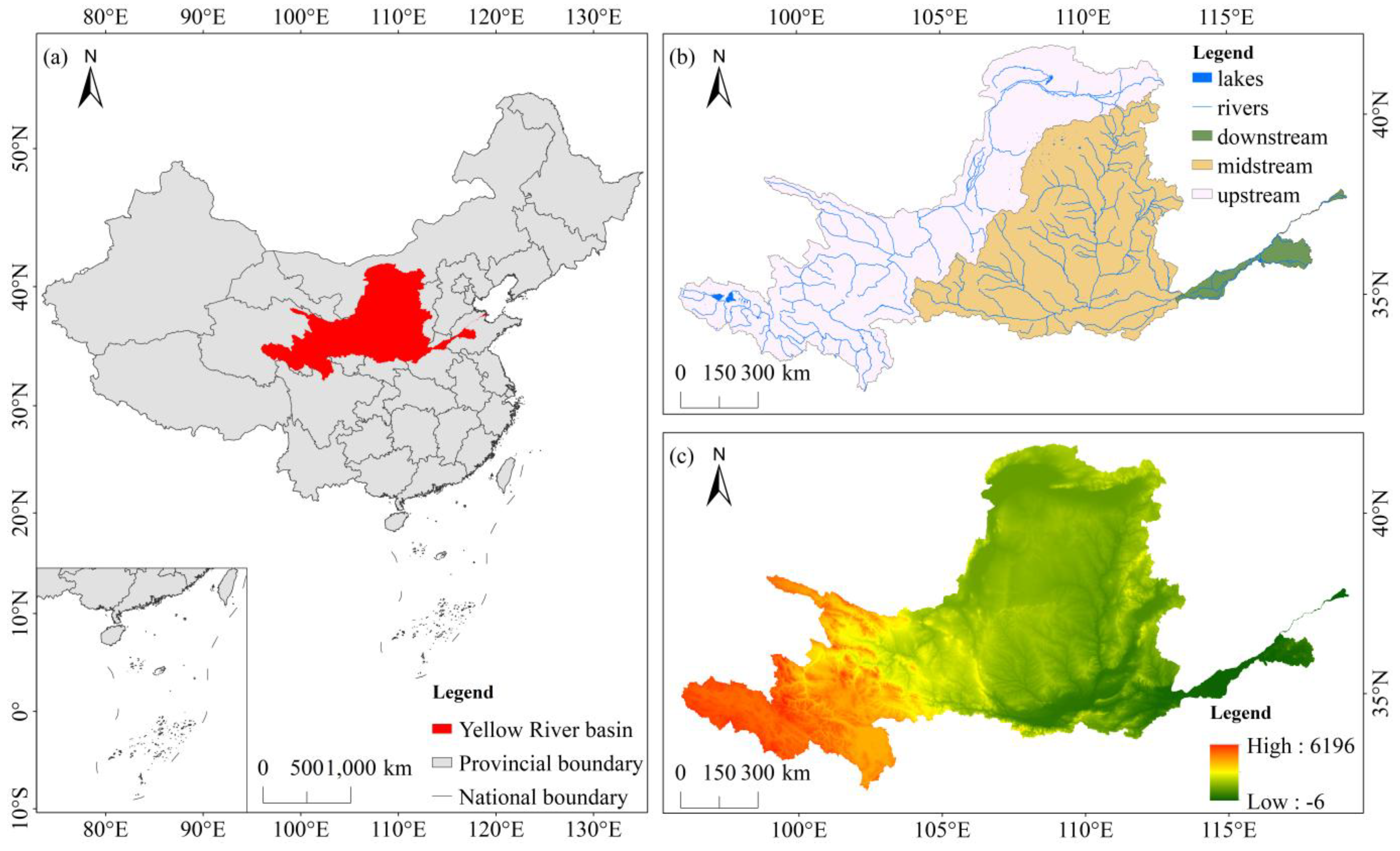
Figure 1. Overview of the YRB: (a) geographic location and spatial extent; (b) sub-basin divisions, including the upper, middle, and lower reaches, and the river network; (c) distribution of elevation.
Land 15 01379 g001
Figure 2. Study workflow for EEQ hotspot and coldspot detection and driving force analysis in the YRB using GEE.
Land 15 01379 g002
Figure 3. RSEI-Based Ecological index STC structure and Emerging Hot Spot Analysis. The asterisk in “GI*” is part of the variable name and does not denote multiplication.
Land 15 01379 g003
Figure 4. Temporal variation in Global Moran’s I for RSEI in the YRB (2000–2021). Asterisks (**) denote statistical significance at the p < 0.01 level.
Land 15 01379 g004
Figure 5. Spatiotemporal patterns of EEQ hotspot and coldspot dynamics in the YRB (2000–2021).
Land 15 01379 g005
Figure 6. EEQ hotspot and coldspot transitions in the YRB (2000–2010 vs. 2011–2021): Analysis of stability zones and dynamics of hotspot shifts. Classification: 1—Stable hotspot; 2—Emerging hotspot; 3—Hotspot degradation; 4—Stable coldspot; 5—Emerging coldspot; 6—Coldspot improvement; 7—No significant pattern detected. (A) North–south stable hotspot belt across Shanxi Province (Linfen, Lüliang, Taiyuan, and Xinzhou); (B) stable hotspots in the upper reaches (Gannan, Huangnan, Guoluo, and Aba); (C) transitional zone with emerging hotspots around Yan’an, Tongchuan, and Qingyang.
Land 15 01379 g006
Figure 7. EEQ hotspot and coldspot transitions in the YRB (2000–2010 vs. 2011–2021): dynamics of coldspot shifts. Classification: 1—Stable hotspot; 2—Emerging hotspot; 3—Hotspot degradation; 4—Stable coldspot; 5—Emerging coldspot; 6—Coldspot improvement; 7—No significant pattern detected. (A) Transition zone in the central Loess Plateau; (B) coldspot improvement in Bayannur; (C) persistent stable coldspot at the Lüliang–Taiyuan–Jinzhong junction.
Land 15 01379 g007
Figure 8. Sankey diagram of EEQ hotspot and coldspot transitions in the YRB (2000–2010 to 2011–2021).
Land 15 01379 g008
Figure 9. Geodetector q-values for individual and interactive effects of RSEI drivers in 2000, 2010, and 2021. (a) Individual q-values of driving factors for 2000, 2010, and 2021; (bd) interactive q-values for 2000, 2010, and 2021, respectively.
Land 15 01379 g009
Figure 10. Descriptive statistics of MGWR regression coefficients for six RSEI driving factors in 2000, 2010, and 2021: (a) maximum, (b) mean, (c) median, (d) minimum, (e) range, and (f) standard deviation.
Land 15 01379 g010
Figure 11. Spatial distribution of MGWR regression coefficients for FVC, PRE, slope, and TEMP in 2000, 2010, and 2021. Subfigures (a,e,i) FVC; (b,f,j) PRE; (c,g,k) slope; (d,h,l) TEMP, with each column representing 2000, 2010, and 2021, respectively.
Land 15 01379 g011
Table 1. Data sources, spatial resolutions, providers, and access platforms.
Data TypeResolutionSource and Website
MODO9A1500 mGEE (https://developers.google.cn/earth-engine, accessed on 28 July 2026)
MOD11A21000 mGEE (https://developers.google.cn/earth-engine, accessed on 28 July 2026)
MOD13A1500 mGEE (https://developers.google.cn/earth-engine, accessed on 28 July 2026)
DEM30 mGeospatial Data Cloud (https://www.gscloud.cn/)
PRE1000 mChina Meteorological Data Services and Data Center (http://data.cma.cn/data/, accessed on 28 July 2026)
TEMP
GDP and POP1000 mResource and Environmental Science Data Platform (https://www.resdc.cn/findpwd.aspx, accessed on 28 July 2026)
FVC500 mNational Earth System Science Data Center (https://gre.geodata.cn/)
LULC30 mLand use data were obtained from the China Land Cover Dataset (CLCD)
Table 2. Summary of major methodological formulations and corresponding references used in this study.
MethodPurposeMain FormulationReference
RSEIQuantification of EEQPCA-based integration of NDVI, WET, NDBSI and LSTXu (2013) [46]; Xu et al. (2019) [6]
Moran’s ISpatial autocorrelation assessmentGlobal spatial clustering measurementMoran (1950) [47]
EHSAHotspot/coldspot trajectory identificationSpace-time cube based classificationGetis. et al. [51,52]
GDDriver detection and interaction analysisq-statisticWang et al. (2016) [49]
OLSGlobal regression relationshipLinear regression modelWooldridge. et al. (2010) [48]
MGWRSpatially heterogeneous relationshipsMultiscale regression frameworkFotheringham et al. (2017) [50]
Table 3. Proportional distribution of spatiotemporal evolution patterns of EEQ hotspots and coldspots in the YRB (%).
Coldspot and Hotspot TypeUpper ReachesMiddle ReachesLower ReachesAll Reaches
New Hotspot0.301.330.510.77
Consecutive Hotspot1.234.130.582.51
Intensifying Hotspot8.3014.473.6010.97
Persistent Hotspot11.345.071.728.23
Diminishing Hotspot0.130.020.350.09
Sporadic Hotspot12.2712.6419.5812.70
Oscillating Hotspot2.6622.636.3411.75
Historical Hotspot0.0020.010.150.09
New Coldspot0.0020.0020.010.002
Consecutive Coldspot0.0220.030.010.02
Intensifying Coldspot0.100.010.110.06
Persistent Coldspot14.120.2600.9017.52
Diminishing Coldspot18.038.150.0212.97
Sporadic Coldspot2.561.502.162.05
Oscillating Coldspot0.020.220.590.13
Historical Coldspot1.010.490.0230.74
No Pattern Detected27.9129.0563.3629.48
Table 4. Reclassification scheme of EHSA based on EEQ change trends.
SubcategoryOriginal EHSA Types IncludedEcological Interpretation
  • Stable Hotspot
(1)
Persistent Hotspot,
(2)
Consecutive Hotspot
Long-term, stable improvement in ecological conditions
2.
Emerging Hotspot
(3)
New Hotspot,
(4)
Intensifying Hotspot
Newly appeared or intensifying hotspots indicate recent ecological improvement
3.
Hotspot Degradation
(5)
Diminishing Hotspot,
(6)
Historical Hotspot,
Hotspots are weakening or disappearing, suggesting declining improvement or reversal
(7)
Sporadic Hotspot,
(8)
Oscillating Hotspot
Intermittent or unstable hotspots, trend direction is uncertain
4.
Stable Coldspot
(9)
Persistent Coldspot,
(10)
Consecutive Coldspot
Long-term, consistent degradation of ecological conditions
5.
Emerging Coldspot
(11)
New Coldspot,
(12)
Intensifying Coldspot
Newly emerging or strengthening coldspots indicate worsening ecological conditions
6.
Coldspot Improvement
(13)
Diminishing Coldspot,
(14)
Historical Coldspot
Coldspots are weakening, possibly indicating recovery potential
(15)
Sporadic Coldspot,
(16)
Oscillating Coldspot
Unstable or intermittent coldspots, degradation trend is uncertain
7.
No Pattern Detected
(17)
No Pattern Detected
No significant spatial or temporal pattern observed
Table 5. Performance Metrics of MGWR Models in 2000, 2010, and 2021.
Model Parameters200020102021
R-Squared0.890.850.90
Adjusted R-Squared0.890.850.90
AICc5523.337699.384607.86
Sigma-Squared (RSS)0.110.150.10
Table 6. Mean RSEI values across different vegetation coverage levels in 2000, 2010, and 2021.
YearLow Coverage
(0–45%)
Moderate Coverage
(45–60%)
Moderately High Coverage
(60–75%)
High Coverage
(75–100%)
20000.230.370.440.61
20100.300.410.470.61
20210.310.460.540.69
Table 7. Key ecological policies and associated EEQ evolution types in the YRB (2000–2010 and 2011–2021).
PeriodBegin YearPolicy/ProjectMain AreaCore Ecological ImpactEvolution Type
The first
decade
(2000–
2010)
1999Grain for Green ILoess Plateau and mid-reachesForest and grassland restoration;No pattern detected (27.53%)
Stable coldspots
(20.96%)
Stable hotspot
(24.20%)
Emerging hotspot (17.04%)
2000Sanjiangyuan ConservationUpper reacheswetland and grassland recovery;
2003Check Dam PilotLoess Plateausediment reduction
2005Expanded SanjiangyuanUpper reachesBiodiversity increased
The
second decade
(2011–
2021)
2012YRB Comprehensive Plan (Revised)Basin-wideIntegrated soil–water management;No pattern detected (31.67%)
Stable coldspots
(20.63%)
Stable hotspot
(25.89%)
Emerging hotspot (14.62%)
2014Grain for Green IIBasin-wideforest and grassland restoration
2020Poverty-Aligned RestorationLower reachesFragmentation reduction
2023Yellow River Protection LawBasin-wideSDG governance targeted
Table 8. Spatial coupling between ecological restoration projects and EEQ hotspot areas in the YRB.
Ecological Restoration ProjectProject Area (km2)Overlap Hotspot Area (km2)Project Hotspot Ratio (%)
Sanjiangyuan Conservation Project117,115.9254,275.8846.34
Grazing Withdrawal Program408,220.36129,342.6131.68
Grain for Green Program752,832.78335,532.0944.57
Note: The spatial coupling ratio represents the percentage of EEQ improvement hotspot areas located within each ecological restoration project area.
Disclaimer/Publisher’s Note: The statements, opinions and data contained in all publications are solely those of the individual author(s) and contributor(s) and not of MDPI and/or the editor(s). MDPI and/or the editor(s) disclaim responsibility for any injury to people or property resulting from any ideas, methods, instructions or products referred to in the content.