GeoLiquefy-AI: Predicting Soil Liquefaction Potential via Deep Neural Architecture Search in Seismically Active Coastal Zones

Abstract

Earthquake-induced soil liquefaction represents a severe geohazard causing catastrophic infrastructure failure in prone coastal zones, requiring an advanced environmental spatial assessment for their sustainable land-use planning. This study utilizes advanced computational intelligence models to predict earthquake-induced soil liquefaction in Boumerdès, Algeria, an area heavily affected by the 2003 (M_w 6.8) earthquake. Utilizing a comprehensive subsurface database of 1984 geotechnical records encompassing lithology, hydrogeological configurations, and seismic parameters, advanced deep learning frameworks are developed and optimized via automated Neural Architecture Search (NAS). The continuous Factor of Safety (F_s) is calculated to distinguish stable profiles from vulnerable strata, benchmarking conventional ANN and DNN models against NAS-optimized variants (NAS-ANN and NAS-DNN) using a stratified 5-fold cross-validation scheme. The optimized hybrid NAS-DNN framework effectively captured non-linear soil responses, achieving a training correlation coefficient ($R_{train}$) of 0.9518, a validation coefficient ($R_{validation}$) of 0.8843, and a cross-validated mean $R$ of approximately 0.82, demonstrating improved predictive reliability compared to traditional models. Ultimately, this optimal network is embedded into the ‘GeoLiquefy-AI (v1.0)’ interface. To ensure reliability for safety-critical applications, we integrated a SHAP explainable AI framework, validating the model’s geomechanical logic by mapping physical soil-liquefaction dependencies. This deployment-ready tool enables rapid, transparent hazard calculations, providing a scalable platform for seismic microzonation and proactive urban risk mitigation.

1. Introduction

Soil liquefaction is a major Earth surface process and a well-documented geotechnical phenomenon that consists of saturated soils undergoing a significant reduction in shear strength and stiffness under seismic loading, resulting in fluid-like behavior that severely compromises civil infrastructure stability [1]. Beyond its localized structural impacts, liquefaction acts as a destructive earthquake-induced ground failure mechanism that causes widespread regional terrain deformation, altering coastal landscapes and disrupting sustainable land-use planning [2]. Traditionally, this hazard has been evaluated through site-specific engineering tests; however, capturing its dynamic macro-spatial patterns can be significantly enhanced through the integration of remote sensing and Geospatial Artificial Intelligence (GeoAI). Advanced earth observation tools, including Interferometric Synthetic Aperture Radar (InSAR) and high-resolution satellite imagery, provide valuable assets for assessing post-seismic surface deformations—such as lateral spreading and ground subsidence—thereby transforming localized geotechnical risks into actionable spatial datasets for environmental monitoring.

Liquefaction is fundamentally characterized as the loss of shear strength in loose, saturated sands subjected to cyclic loading [3]. The destructive phenomena observed during the 1964 Alaska and Niigata earthquakes served as a critical turning point, transitioning liquefaction research from anecdotal observation to a rigorous discipline within geotechnical earthquake engineering. Consequently, assessing liquefaction susceptibility has become a fundamental component of land system science and seismic risk mapping. The simplified procedure pioneered by Seed and Idriss, which evaluates the Factor of Safety (FS) by comparing Cyclic Resistance Ratio (CRR) to Cyclic Stress Ratio (CSR), has evolved into a global standard for site-specific hazard assessment [4]. Today, these empirical foundations are integrated into modern deep learning algorithms, providing a robust computational pathway to rapidly predict liquefaction potential based on extensive subsurface records.

Among the most significant case studies, the 1995 Kobe earthquake in Japan stands as a benchmark event for liquefaction investigations, particularly regarding its profound impact on reclaimed and coastal land-use systems [5]. The extensive liquefaction experienced by these high-density urban areas caused severe settlements, lateral spreading, and critical infrastructure damage, highlighting the inherent vulnerability of anthropogenically altered coastal terrains. This event served as a catalyst for the development and validation of modern liquefaction assessment techniques, shifting the paradigm from purely empirical observations toward robust, data-driven, and machine-learning-based approaches that can now support large-scale spatial decision-making and sustainable landscape management.

At the regional scale, the northern tectonic margin of Algeria exhibits high vulnerability to earthquake-induced terrain dynamics, having experienced significant liquefaction-induced damage during major seismic events. Notably, the 1980 El Asnam (Chlef) earthquake (M_w 7.3) and the destructive 2003 Boumerdes earthquake generated widespread ground failures, including lateral spreading and significant differential settlements within young alluvial and coastal deposits [6]. During the 2003 Boumerdes event, liquefaction phenomena were extensively triggered across coastal zones and unconsolidated sandy formations, leading to severe surface deformation and structural failures along the littoral infrastructure. These historical precedents confirm that liquefaction constitutes a major environmental and seismic hazard in North African coastal plains, which are characterized by highly vulnerable geological configurations and complex geotechnical conditions. Consequently, understanding these earth surface responses has been the focus of numerous post-seismic studies and hazard microzonation frameworks conducted by regional researchers [6,7].

In geotechnical and environmental engineering practice, land susceptibility to liquefaction is commonly evaluated using in situ subsurface testing, such as the Standard Penetration Test (SPT), Cone Penetration Test (CPT), and Pressuremeter Test (PMT). These traditional approaches estimate the seismic loading demand via the Cyclic Stress Ratio (CSR) and the soil shear capacity via the Cyclic Resistance Ratio (CRR) to calculate the localized Factor of Safety (FS). Early empirical models relied primarily on univariate empirical models, which were subsequently extended to CPT tip resistance and geophysical shear wave velocity ($V_s$)-based approaches. Over the past decades, empirical and semi-empirical procedures have been continually updated to incorporate environmental and geological correction factors, including overburden effective stress, fines content (FC), earthquake magnitude, and localized site conditions. Among the most widely adopted foundational frameworks are those developed by Seed et al. [4,8]; they were later refined to reduce prediction uncertainties [9]. Additionally, non-invasive geophysical techniques based on V_s profile logging have gained increasing attention for mapping structural soil stiffness and dynamic properties without terrain disruption, particularly within densely populated urban zones and seismically active coastal landscapes.

Despite the continuous refinement of empirical and semi-empirical formulations, their predictive capability remains significantly constrained by the highly non-linear behavior of dynamic soil systems, parameter uncertainties, and pronounced site-specific geomorphological variability [10]. In the context of heterogeneous land systems, the traditional deterministic Factor of Safety (FS) often fails to serve as a definitive binary indicator for liquefaction triggering. Specifically, an FS < 1 does not inherently guarantee terrain stability against non-liquefaction, nor does an FS > 1 systematically imply catastrophic ground failure [11]. These discrepancies arise because deterministic boundaries struggle to integrate critical macro-environmental factors. Additional structural uncertainties—stemming from multi-layered soil stratigraphy, localized correction factors, and the complex depositional environments of young coastal alluvial basins—further degrade macro-spatial prediction accuracy and limit model transferability across distinct geological regions [12,13].

To overcome the rigidity of deterministic boundaries, probabilistic approaches based on liquefaction probability (P_L) have been increasingly adopted to better quantify regional seismic risk and landscape vulnerability. Because liquefaction frequently develops within highly stratified and multi-layered soil deposits, its initiation at depth can propagate upward, resulting in massive earth surface deformation and severe infrastructure failure at the ground level [14]. These probabilistic frameworks have been extensively validated using historical databases encompassing both liquefied and non-liquefied sites across diverse geological settings [15,16,17,18,19,20,21,22]. Among these, multivariate logistic regression models have been widely employed to map spatial hazard uncertainty. For instance, Chung and Rogers (2017) proposed a foundational statistical relationship for estimating regional liquefaction probability, formulated as follows [23]:

$$P={\displaystyle \frac{1}{1+e^{-(B_0+B_{1}X)}}}$$

(1)

where P represents the probability of localized liquefaction occurrence, X denotes the selected geotechnical or seismic predictor variable, $B_0$ is the statistical intercept term, and $B_1$ corresponds to the calculated regression coefficient. While these parametric probabilistic methods improve risk characterization compared to binary methods, they are structurally limited when processing multi-source geospatial big data characterized by extreme non-linearity and heterogeneous spatial dimensions.

To overcome these spatial limitations, regional hazard microzonation can be significantly enhanced by integrating non-invasive surface characterization techniques, including seismic refraction, seismic reflection, ambient vibration measurements, and recorded ground motion analyses. Among these spectral approaches, the Horizontal-to-Vertical Spectral Ratio (H/V) technique, commonly known as the Nakamura method, is widely deployed to estimate the fundamental resonance frequency of surficial soil deposits and evaluate localized site amplification effects without terrain disruption [24]. In the specific case of the 2003 Boumerdes earthquake, comprehensive post-disaster field investigations demonstrated that coastal areas composed of soft quaternary alluvium and unconsolidated marine sediments experienced severe amplification of seismic waves, resulting in higher damage density patterns compared to more competent geological formations [25,26]. These findings highlight the importance of integrating geophysical and geotechnical approaches for seismic microzonation and liquefaction susceptibility assessment [27].

In parallel, advanced numerical-based methods have become essential computational tools for simulating liquefaction behavior under dynamic seismic loading. Unlike semi-empirical formulations, these numerical techniques explicitly model highly non-linear soil-structure interactions, transient pore water pressure generation, and large plastic deformation mechanisms. Finite Element Method (FEM) and Finite Difference Method (FDM) frameworks—implemented in specialized geomechanics platforms such as PLAXIS 2D/3D, FLAC, and ABAQUS—enable detailed, physics-based simulations of site-specific boundary conditions, including complex soil stratification and local topographic effects. Previous boundary-value studies have demonstrated that these numerical simulations can successfully reproduce the macroscopic and microscopic characteristics of saturated granular soil behavior during cyclic shearing when rigorously validated against physical shaking table experiments and centrifuge tests [28]. However, from a land system management perspective, the extreme computational cost, parameter-heavy constitutive models, and localized focus of these deterministic simulations restrict their applicability for real-time, regional-scale environmental monitoring and macro-spatial hazard prediction.

Despite these engineering advances, conventional semi-empirical and deterministic numerical approaches still face systemic limitations related to robust uncertainty quantification, extreme computational costs, and the convoluted characterization of non-linear soil-structure interactions [29]. Consequently, recent paradigm shifts in Machine Learning (ML) and Artificial Intelligence (AI) have provided powerful, scalable alternatives for macro-spatial liquefaction susceptibility assessment [7,30,31,32,33,34,35,36,37]. Unlike traditional empirical models, advanced ML techniques can efficiently ingest and process large, high-dimensional, and heterogeneous datasets—seamlessly integrating multi-source geological, geotechnical, seismic, and spatial information to automatically map the dominant controlling factors of dynamic soil failure [38]. Modern computational algorithms, such as Artificial Neural Networks (ANN), Support Vector Machines (SVM), decision tree-based ensembles, and Deep Neural Networks (DNN), have demonstrated superior fidelity in modeling complex, multivariate, and highly non-linear relationships under dynamic environmental boundary conditions [7,30,31,32,33,34,35,36,37]. Furthermore, recent advancements have shifted towards integrating explainable machine learning (EML) techniques to bridge the gap between black-box computational intelligence and traditional domain knowledge. For instance, Jas et al. (2024) developed an explainable LightGBM-SHAP model for gravelly soil liquefaction, demonstrating that integrating SHapley Additive exPlanations (SHAP) can align data-driven predictions with established geomechanical principles, thereby enhancing the transparency and reliability of liquefaction hazard assessments [39]. Recent advancements in geotechnical engineering highlight a paradigm shift towards integrating geomechanical domain knowledge with hybrid deep learning frameworks, enabling more precise, probabilistic assessments of complex soil-structure interactions in spatially variable environments [40,41].

Numerous recent studies have validated the robustness of these computational intelligence frameworks and demonstrated the effectiveness of machine learning frameworks for liquefaction-related applications. For instance, Sargın et al. (2026) developed machine learning models for estimating liquefaction-induced settlement of shallow foundations using an imbalanced dataset and achieved high prediction accuracy [38]. Similarly, Xue and Xiao (2016) deployed hybrid SVM algorithms to interpret standard penetration parameters, reporting excellent classification boundary verification [42]. Concurrently, Zhu et al. (2017) highlighted the resilience of ensemble tree-based configurations, emphasizing their exceptional robustness when handling noisy, missing, or highly heterogeneous regional geotechnical datasets [43]. More recently, decision-tree paradigms have shown promising performance for decoding SPT sequences in complex geological formations [44]. Furthermore, to bridge the gap between data-driven accuracy and risk-informed urban engineering, Bayesian Belief Networks (BBN) have been increasingly synthesized with deep learning approaches to capture stochastic spatial variability and enhance probabilistic hazard microzonation workflows [45,46]. To provide a comprehensive synthesis of the recent advancements in computational intelligence for soil failure prediction, a rigorous benchmarking of existing literature is compiled and presented in Table 1.

Based on a comprehensive synthesis of the compiled literature, several critical research gaps and methodological limitations persist in current machine learning-based soil liquefaction predictive models. Primarily, the first research gap relates to algorithmic constraints; a significant majority of existing frameworks remain heavily reliant on conventional machine learning algorithms—such as standard Artificial Neural Networks (ANN) or Support Vector Machines (SVM). These models are inherently constrained by their dependence on manual hyperparameter tuning and their vulnerability to local optimization constraints. Furthermore, a major research gap exists regarding the scale of the geospatial and geotechnical databases utilized in previous research. As outlined in Table 1, even the most robust studies rarely exceed 834 borehole samples. This restriction significantly induces epistemic uncertainty and limits model generalization across heterogeneous coastal domains. This challenge is compounded by a widespread absence of advanced stochastic verification protocols, such as stratified k-fold cross-validation, leaving existing models highly susceptible to hidden overfitting risks. Finally, a profound disconnection remains between data-driven modeling and field engineering practice. Published frameworks typically deliver abstract mathematical outputs or static weight matrices rather than deployment-ready tools. The absence of user-friendly Graphical User Interfaces (GUIs) designed for real-time, on-site prediction highlights the ultimate research gap that this study directly addresses.

To effectively address these persistent methodological gaps, the present study introduces a data-driven framework that bridges the gap between advanced computational intelligence and practical landslide and ground-failure hazard mitigation. Primarily, this research deploys an automated, hybrid Neural Architecture Search Deep Neural Network (NAS-DNN) approach—an advanced AutoML paradigm that has demonstrated high predictive accuracy and stable performance in solving nonlinear geotechnical engineering problems [47,48,49,50]. To eliminate the constraints of limited datasets, a comprehensive regional database comprising 1984 multi-source spatial and subsurface records from the seismically active coastal zone of Boumerdes, Algeria, was meticulously compiled and processed. Furthermore, to rigorously safeguard the predictive model against hidden overfitting and underfitting phenomena, a stratified 5-fold cross-validation verification protocol was systematically executed, ensuring high generalization performance across distinct heterogeneous geological layers. Finally, to transition these abstract machine learning mathematical frameworks into deployment-ready engineering applications, the optimized model was successfully embedded into an intuitive, user-friendly Graphical User Interface (GUI). This decision-support tool is specifically designed to enable field geotechnical engineers to perform instantaneous, reliable, on-site liquefaction factor of safety (FS) predictions, while simultaneously serving as a foundational geospatial baseline for constructing dynamic regional macro-susceptibility hazard maps and sustainable coastal urban planning frameworks in the future.

Table 1. Comprehensive comparative summary of published computational intelligence models for soil liquefaction prediction versus the proposed automated deep learning framework.

References	Model Used	Input Parameters	Samples
[51]	SVM	$\mathrm{Depth} (z$$), \mathrm{Cone} \mathrm{tip} \mathrm{resistance} (q_c$$), \mathrm{Sleeve} \mathrm{friction} (f_s$$), \mathrm{Pore} \mathrm{water} \mathrm{pressure} (u$$), \mathrm{Friction} \mathrm{ratio} (R_f$$), \mathrm{Total} \mathrm{overburden} \mathrm{stress} ({\sigma }_v$$), \mathrm{Effective} \mathrm{overburden} \mathrm{stress} ({{\sigma }_v}^{\prime }$$), \mathrm{Normalized} \mathrm{cone} \mathrm{resistance} (Q_{tn}$$), \mathrm{Peak} \mathrm{ground} \mathrm{acceleration} (a_{max}$$), \mathrm{and} \mathrm{Cyclic} \mathrm{Stress} \mathrm{Ratio} (CSR$)	134
[52]	XGB, GBM, RF, SVR, GMDH	$\mathrm{Corrected} \mathrm{SPT} \mathrm{blow} \mathrm{count} ({\left(N_1\right)}_{60}$$), \mathrm{Fines} \mathrm{content} (FC$$), \mathrm{Peak} \mathrm{ground} \mathrm{acceleration} (a_{max}$$), \mathrm{Total} \mathrm{overburden} \mathrm{stress} ({\sigma }_v$$), \mathrm{Effective} \mathrm{overburden} \mathrm{stress} ({{\sigma }_v}^{\prime }$$), \mathrm{and} \mathrm{Earthquake} \mathrm{magnitude} (M_w$)	620
[53]	SVM, RF, XGB	$\mathrm{Shear} \mathrm{wave} \mathrm{velocity} (V_s$$), \mathrm{Effective} \mathrm{overburden} \mathrm{stress} ({{\sigma }_v}^{\prime }$$), \mathrm{Groundwater} \mathrm{table} \mathrm{depth} (d_w$$), \mathrm{Total} \mathrm{overburden} \mathrm{stress} ({\sigma }_v$$), \mathrm{Effective} \mathrm{overburden} \mathrm{stress} ({{\sigma }_v}^{\prime }$$), \mathrm{Surface} \mathrm{peak} \mathrm{horizontal} \mathrm{acceleration} (a_{max}$$), \mathrm{Cyclic} \mathrm{Stress} \mathrm{Ratio} (CSR$$), \mathrm{Earthquake} \mathrm{magnitude} (M_w$$), \mathrm{and} \mathrm{Stress} \mathrm{reduction} \mathrm{coefficient} (r_d$)	415
[54]	DNN	$\mathrm{Corrected} \mathrm{SPT} \mathrm{blow} \mathrm{count} ({\left(N_1\right)}_{60}$$), \mathrm{Fines} \mathrm{content} (FC$$), \mathrm{Peak} \mathrm{ground} \mathrm{acceleration} (a_{max}$$), \mathrm{Total} \mathrm{overburden} \mathrm{stress} ({\sigma }_v$$), \mathrm{Effective} \mathrm{overburden} \mathrm{stress} ({{\sigma }_v}^{\prime }$$), \mathrm{Earthquake} \mathrm{magnitude} (M_w$$), \mathrm{Depth} (z$$), \mathrm{and} \mathrm{Shear} \mathrm{wave} \mathrm{velocity} (V_s$)	556
[55]	BP, SVM, DT, and KNN	$\mathrm{Corrected} \mathrm{SPT} \mathrm{blow} \mathrm{count} ({\left(N_1\right)}_{60}$$), \mathrm{Fines} \mathrm{content} (FC$$), \mathrm{Peak} \mathrm{ground} \mathrm{acceleration} (a_{max}$$), \mathrm{Total} \mathrm{overburden} \mathrm{stress} ({\sigma }_v$$), \mathrm{Effective} \mathrm{overburden} \mathrm{stress} ({{\sigma }_v}^{\prime }$$), \mathrm{Earthquake} \mathrm{magnitude} (M_w$$), \mathrm{Depth} (z$$), \mathrm{Shear} \mathrm{wave} \mathrm{velocity} (V_s$$), \mathrm{Groundwater} \mathrm{table} \mathrm{depth} (d_w$$), \mathrm{and} \mathrm{Internal} \mathrm{friction} \mathrm{angle} (\varphi$)	620
[56]	ANN-ABC, ANN-TLBO, ANN-ALO, ANN-ACO, ANN-ICA, ANN-SCE	$\mathrm{Corrected} \mathrm{SPT} \mathrm{blow} \mathrm{count} ({\left(N_1\right)}_{60}$$), \mathrm{Fines} \mathrm{content} (FC$$), \mathrm{Peak} \mathrm{ground} \mathrm{acceleration} (a_{max}$$), \mathrm{Total} \mathrm{overburden} \mathrm{stress} ({\sigma }_v$$), \mathrm{Effective} \mathrm{overburden} \mathrm{stress} ({{\sigma }_v}^{\prime }$$), \mathrm{Earthquake} \mathrm{magnitude} (M_w$$), \mathrm{and} \mathrm{Depth} (z$)	834
[57]	DNN, CNN, LSTM, RNN, BILSTM	$\mathrm{Corrected} \mathrm{SPT} \mathrm{blow} \mathrm{count} ({\left(N_1\right)}_{60}$$), \mathrm{Fines} \mathrm{content} (FC$$), \mathrm{Peak} \mathrm{ground} \mathrm{acceleration} (a_{max}$$), \mathrm{Total} \mathrm{overburden} \mathrm{stress} ({\sigma }_v$$), \mathrm{and} \mathrm{Effective} \mathrm{overburden} \mathrm{stress} ({{\sigma }_v}^{\prime }$)	834
Our Study	ANN, NAS-ANN, NAS- DNN	$\mathrm{Depth} (z$$), \mathrm{Lithology} \mathrm{code}, \mathrm{Bulk} \mathrm{wet} \mathrm{density} ({\gamma }_h$$), \mathrm{Gravimetric} \mathrm{water} \mathrm{content} (w$$), \mathrm{Degree} \mathrm{of} \mathrm{saturation} (S_r$$), \mathrm{Fines} \mathrm{content} (FC$$), \mathrm{Total} \mathrm{overburden} \mathrm{stress} ({\sigma }_v$$), \mathrm{Effective} \mathrm{overburden} \mathrm{stress} ({{\sigma }_v}^{\prime }$$), \mathrm{Cyclic} \mathrm{Stress} \mathrm{Ratio} (CSR$$), \mathrm{and} \mathrm{Normalized} \mathrm{peak} \mathrm{ground} \mathrm{acceleration} (a_{max}/g$)	1984

Table 1. Comprehensive comparative summary of published computational intelligence models for soil liquefaction prediction versus the proposed automated deep learning framework.

References	Model Used	Input Parameters	Samples
[51]	SVM	$\mathrm{Depth} (z$$), \mathrm{Cone} \mathrm{tip} \mathrm{resistance} (q_c$$), \mathrm{Sleeve} \mathrm{friction} (f_s$$), \mathrm{Pore} \mathrm{water} \mathrm{pressure} (u$$), \mathrm{Friction} \mathrm{ratio} (R_f$$), \mathrm{Total} \mathrm{overburden} \mathrm{stress} ({\sigma }_v$$), \mathrm{Effective} \mathrm{overburden} \mathrm{stress} ({{\sigma }_v}^{\prime }$$), \mathrm{Normalized} \mathrm{cone} \mathrm{resistance} (Q_{tn}$$), \mathrm{Peak} \mathrm{ground} \mathrm{acceleration} (a_{max}$$), \mathrm{and} \mathrm{Cyclic} \mathrm{Stress} \mathrm{Ratio} (CSR$)	134
[52]	XGB, GBM, RF, SVR, GMDH	$\mathrm{Corrected} \mathrm{SPT} \mathrm{blow} \mathrm{count} ({\left(N_1\right)}_{60}$$), \mathrm{Fines} \mathrm{content} (FC$$), \mathrm{Peak} \mathrm{ground} \mathrm{acceleration} (a_{max}$$), \mathrm{Total} \mathrm{overburden} \mathrm{stress} ({\sigma }_v$$), \mathrm{Effective} \mathrm{overburden} \mathrm{stress} ({{\sigma }_v}^{\prime }$$), \mathrm{and} \mathrm{Earthquake} \mathrm{magnitude} (M_w$)	620
[53]	SVM, RF, XGB	$\mathrm{Shear} \mathrm{wave} \mathrm{velocity} (V_s$$), \mathrm{Effective} \mathrm{overburden} \mathrm{stress} ({{\sigma }_v}^{\prime }$$), \mathrm{Groundwater} \mathrm{table} \mathrm{depth} (d_w$$), \mathrm{Total} \mathrm{overburden} \mathrm{stress} ({\sigma }_v$$), \mathrm{Effective} \mathrm{overburden} \mathrm{stress} ({{\sigma }_v}^{\prime }$$), \mathrm{Surface} \mathrm{peak} \mathrm{horizontal} \mathrm{acceleration} (a_{max}$$), \mathrm{Cyclic} \mathrm{Stress} \mathrm{Ratio} (CSR$$), \mathrm{Earthquake} \mathrm{magnitude} (M_w$$), \mathrm{and} \mathrm{Stress} \mathrm{reduction} \mathrm{coefficient} (r_d$)	415
[54]	DNN	$\mathrm{Corrected} \mathrm{SPT} \mathrm{blow} \mathrm{count} ({\left(N_1\right)}_{60}$$), \mathrm{Fines} \mathrm{content} (FC$$), \mathrm{Peak} \mathrm{ground} \mathrm{acceleration} (a_{max}$$), \mathrm{Total} \mathrm{overburden} \mathrm{stress} ({\sigma }_v$$), \mathrm{Effective} \mathrm{overburden} \mathrm{stress} ({{\sigma }_v}^{\prime }$$), \mathrm{Earthquake} \mathrm{magnitude} (M_w$$), \mathrm{Depth} (z$$), \mathrm{and} \mathrm{Shear} \mathrm{wave} \mathrm{velocity} (V_s$)	556
[55]	BP, SVM, DT, and KNN	$\mathrm{Corrected} \mathrm{SPT} \mathrm{blow} \mathrm{count} ({\left(N_1\right)}_{60}$$), \mathrm{Fines} \mathrm{content} (FC$$), \mathrm{Peak} \mathrm{ground} \mathrm{acceleration} (a_{max}$$), \mathrm{Total} \mathrm{overburden} \mathrm{stress} ({\sigma }_v$$), \mathrm{Effective} \mathrm{overburden} \mathrm{stress} ({{\sigma }_v}^{\prime }$$), \mathrm{Earthquake} \mathrm{magnitude} (M_w$$), \mathrm{Depth} (z$$), \mathrm{Shear} \mathrm{wave} \mathrm{velocity} (V_s$$), \mathrm{Groundwater} \mathrm{table} \mathrm{depth} (d_w$$), \mathrm{and} \mathrm{Internal} \mathrm{friction} \mathrm{angle} (\varphi$)	620
[56]	ANN-ABC, ANN-TLBO, ANN-ALO, ANN-ACO, ANN-ICA, ANN-SCE	$\mathrm{Corrected} \mathrm{SPT} \mathrm{blow} \mathrm{count} ({\left(N_1\right)}_{60}$$), \mathrm{Fines} \mathrm{content} (FC$$), \mathrm{Peak} \mathrm{ground} \mathrm{acceleration} (a_{max}$$), \mathrm{Total} \mathrm{overburden} \mathrm{stress} ({\sigma }_v$$), \mathrm{Effective} \mathrm{overburden} \mathrm{stress} ({{\sigma }_v}^{\prime }$$), \mathrm{Earthquake} \mathrm{magnitude} (M_w$$), \mathrm{and} \mathrm{Depth} (z$)	834
[57]	DNN, CNN, LSTM, RNN, BILSTM	$\mathrm{Corrected} \mathrm{SPT} \mathrm{blow} \mathrm{count} ({\left(N_1\right)}_{60}$$), \mathrm{Fines} \mathrm{content} (FC$$), \mathrm{Peak} \mathrm{ground} \mathrm{acceleration} (a_{max}$$), \mathrm{Total} \mathrm{overburden} \mathrm{stress} ({\sigma }_v$$), \mathrm{and} \mathrm{Effective} \mathrm{overburden} \mathrm{stress} ({{\sigma }_v}^{\prime }$)	834
Our Study	ANN, NAS-ANN, NAS- DNN	$\mathrm{Depth} (z$$), \mathrm{Lithology} \mathrm{code}, \mathrm{Bulk} \mathrm{wet} \mathrm{density} ({\gamma }_h$$), \mathrm{Gravimetric} \mathrm{water} \mathrm{content} (w$$), \mathrm{Degree} \mathrm{of} \mathrm{saturation} (S_r$$), \mathrm{Fines} \mathrm{content} (FC$$), \mathrm{Total} \mathrm{overburden} \mathrm{stress} ({\sigma }_v$$), \mathrm{Effective} \mathrm{overburden} \mathrm{stress} ({{\sigma }_v}^{\prime }$$), \mathrm{Cyclic} \mathrm{Stress} \mathrm{Ratio} (CSR$$), \mathrm{and} \mathrm{Normalized} \mathrm{peak} \mathrm{ground} \mathrm{acceleration} (a_{max}/g$)	1984

2. Geotechnical Database and Computational Methodology

2.1. Geographic and Geotectonic Setting of the Study Area

The Boumerdes region, situated within the northeastern margin of the Mitidja Basin in northern Algeria (longitudes 2°52′24″ E to 2°58′18″ E and latitudes 36°39′29″ N to 36°44′52″ N), represents a highly dynamic coastal landscape characterized by a complex geological, geotechnical, and hydrogeological evolution. The subsurface stratigraphy is predominantly composed of heterogeneous quaternary sedimentary formations, including interbedded soft clays, silts, unconsolidated sands, marls, and localized limestone lenses. These formations exhibit highly variable spatial thicknesses and mechanical facies that directly govern local soil stiffness and non-linear seismic site response. Tectonically, the coastal plain is intensely active, intersected by an intricate network of blind faults and quaternary folds driven by the ongoing compressional convergence between the African and Eurasian plates. This structural configuration renders the region highly susceptible to destructive seismic disruptions, as epitomized by the historical 1954 Chlef earthquake (M_w 6.7) and numerous moderate regional events that characterize northern Algeria’s persistent seismic hazard profile [58].

From a geotechnical and hydrogeological standpoint, the shallow lithological profiles consist of loose, saturated sandy formations and soft alluvial deposits that display extreme vulnerability to earthquake-induced liquefaction triggering [59]. The hydrogeological domain comprises a complex dual system: an unconfined, shallow water table hosting groundwater primarily within porous gravelly-sandy layers, and deeper, confined aquifers bounded by dense sandy-gravelly complexes. The presence of a persistently shallow groundwater table considerably magnifies liquefaction susceptibility during strong seismic events by promoting rapid excess pore water pressure buildup. 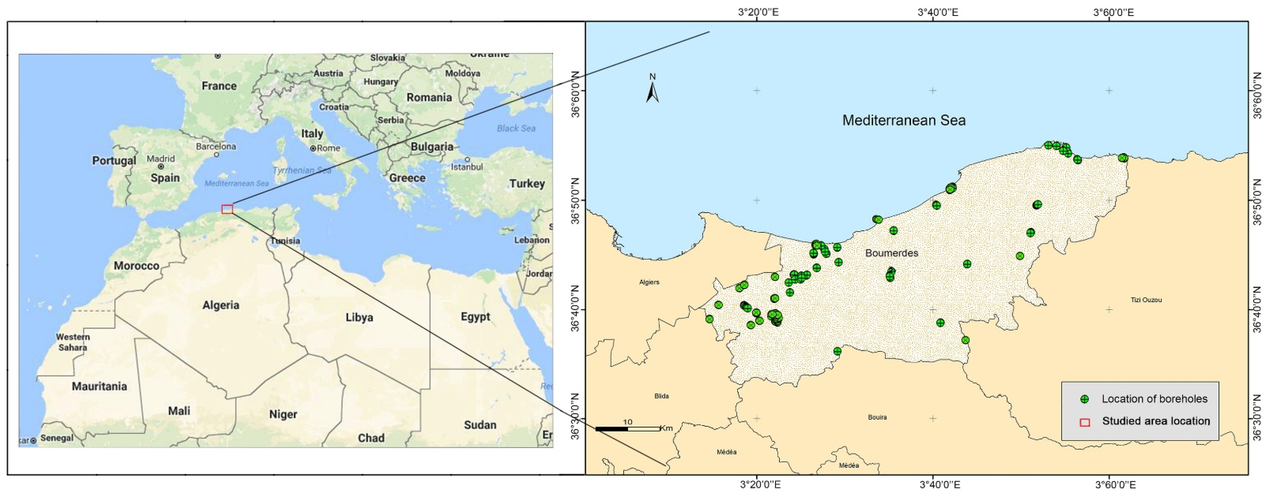The high spatial heterogeneity of these soil matrices, combined with local fault lineations, heavily dictates groundwater flow trajectories and local wave amplification, underscoring the critical need for integrating data-driven Geospatial Artificial Intelligence models into regional microzonation and urban land-use planning frameworks [60]. In order to provide a clear seismotectonic and geographic context, the boundary configurations of the coastal study area in northern Algeria, alongside the georeferenced spatial positioning of the field investigation boreholes, are mapped and delineated in Figure 1.

2.2. Seismotectonic Trigger: The 2003 Boumerdes Earthquake

The contemporary imperative for hazard mapping in this region is dictated by the devastating M_w 6.8 Boumerdes earthquake, which struck northern Algeria on May 21, 2003. Centered offshore approximately 7 km north of the Zemmouri maritime village, the rupture occurred along a previously unmapped, hidden reverse fault system, as validated by seismic network monitoring [59]. Moment tensor configurations revealed a shallow reverse faulting mechanism (<10 km depth) matching the regional compressional stress fields. The shock propagated severe ground motions that reached a maximum intensity of X on the MSK scale, culminating in catastrophic terrain failure, horizontal lateral spreading, and severe differential settlements across coastal sandy formations. This seismic disaster caused approximately 2300 fatalities, over 11,000 injuries, and displaced nearly 200,000 residents, establishing it as one of the most destructive environmental and structural geohazards in the modern history of the western Mediterranean [59].

2.3. Geotechnical Database Architecture and Spatial Layout

To capture the complex subsurface dynamics of the Boumerdes coastal plain, a massive subsurface database was constructed by archiving a total of 1984 geotechnical records spanning four decades of field investigations. The data inventory comprises two distinct investigation techniques: cored boreholes providing continuous stratigraphic core profiles, and destructive penetration/pressuremeter test boreholes evaluating mechanical strength properties. In terms of spatial metadata integration, a common real-world data constraint was encountered: a subset of the archival borehole records lacked explicit geographic coordinate logging due to the historical nature of older investigations. To ensure rigorous spatial modeling, these multi-source records were bifurcated during the data preprocessing stage. The sub-dataset possessing precise spatial metadata was georeferenced and projected to map the physical layout of the investigation sites, as illustrated in the regional borehole location map (Figure 1). For the broader machine learning training phase, the entire database of 1984 tabular geotechnical layers was utilized, enabling the hybrid deep learning engine to decode the internal mechanical and physical cross-correlations governing liquefaction factor of safety equations across highly diverse stratigraphic contexts.

2.4. Foundational Formulation of Soil Liquefaction Evaluation

To evaluate the triggering potential of seismic soil liquefaction across the heterogeneous strata of the Boumerdes region, the conventional simplified procedure was adopted. In this framework, the deterministic Factor of Safety (Fs) against liquefaction triggering is defined as the ratio between the soil’s capacity to resist cyclic shearing—expressed as the Cyclic Resistance Ratio (CRR_7.5) adjusted for a benchmark earthquake magnitude of M_w = 7.5 and the seismic loading demand induced by the earthquake, designated as the Cyclic Stress Ratio (CSR). The Factor of Safety (FS) against liquefaction was estimated using the simplified empirical procedure originally proposed by Seed and Idriss [1] and subsequently refined by Boulanger and Idriss [15]. These equations are widely adopted in engineering practice for liquefaction triggering assessment and represent empirical correlations derived from laboratory testing, field observations, and documented case histories rather than analytical solutions based on fundamental soil mechanics.

$$Fs ={\displaystyle \frac{{CRR}_{7.5}}{CSR}} MSF$$

(2)

where FS is the factor of safety against liquefaction, CRR_7.5 is the cyclic resistance ratio for a reference earthquake of moment magnitude M_w = 7.5, CSR is the cyclic stress ratio, and MSF is the Magnitude Scaling Factor, which accounts for the influence of earthquake magnitude on liquefaction resistance. Following the recommendations of the Algerian Seismic Code (RPA 2024), the reference earthquake magnitude is M_w = 7.5; therefore, MSF = 1.0 was adopted throughout this study.

The Cyclic Stress Ratio (CSR), which represents the earthquake-induced cyclic shear stress normalized by the initial Effective overburden stress, was calculated as

$$CSR=0.65 \left({\displaystyle \frac{a_{max}}{g}}\right)\left({\displaystyle \frac{{\sigma v}_0}{{\sigma }^{\prime }v}}\right) rd$$

(3)

where

• a_max is the peak horizontal ground acceleration at the ground surface (g);
• g is the gravitational acceleration;
• σ_v0 is the total overburden stress (kPa);
• σ′_v is the effective overburden stress (kPa);
• rd is the depth-dependent stress reduction coefficient accounting for soil deformability.

The stress reduction coefficient rd was estimated using the empirical relationship proposed by Seed and Idriss:

$$r_d=\left\{\begin{array}{c}1.0-0.00765 z for z \le 9.15 m\\ 1.174-0.0267 z for 9.15\le z\le 23 m\end{array}\right.$$

(4)

To evaluate the soil’s cyclic capacity, field penetration records from the Standard Penetration Test (SPT) are normalized. The standardized SPT blow count (N₆₀), corrected for energy efficiency and borehole boundary conditions, is expressed as [22]

$$N_{60}=N_{SPT }{C}_{N }{C}_E{C}_B{C}_S$$

(5)

Consequently, the Cyclic Resistance Ratio (CRR) is derived based on the corrected clean-sand equivalent blow count ((N₁) _60cs), incorporating adjustments for the soil’s fines content (FC). The cyclic resistance ratio ($CR{R}_{7.5}$) was calculated using the SPT-based relationship adopted in the Algerian Seismic Code (RPA 2024), according to the NCEER method proposed by Youd et al. (2001) [22]:

$$CRR = {\displaystyle \frac{1}{34-{N1}_{60CS}}}+{\displaystyle \frac{{N1}_{60}}{135}}+ {\displaystyle \frac{50}{{{\left(10\right(N1)}_{60cs}+45)}^2}}-{\displaystyle \frac{1}{200}}$$

(6)

2.5. Feature Engineering and Physics-Based Variables Configuration

Within the proposed automated deep learning framework, ten key physical and environmental indicators were selected as primary input features (X₁ to X₁₀) to train the automated hybrid deep learning engine. The physical significance and geotechnical control of each parameter are presented in

Table 2. Explicit feature configuration, operational definitions, and mathematical notation of the input and output variables deployed in the hybrid machine learning model.

Code	Parameter Type	Parameter Name	Abbrev. & Symbol	Unit
X1	Quantitative	Borehole Sample Depth	z	m
X2	Qualitative (Categorical)	Lithological Stratum Facies	Code 1–13	Dimensionless
X3	Quantitative	Soil Bulk Wet Density	γh	t/m3
X4	Quantitative	Natural Gravimetric Water Content	w	%
X5	Quantitative	Volumetric Degree of Saturation	Sr	%
X6	Quantitative	Fine Fraction (<0.08 mm)	FC	%
X7	Quantitative	Total Overburden Stress	σv	kPa
X8	Quantitative	Effective overburden stress	σv′	kPa
X9	Quantitative	Dynamic Cyclic Stress Ratio	CSR	Dimensionless
X10	Quantitative	Peak Horizontal Ground Acceleration Ratio	amax/g	Dimensionless
Y	Quantitative	Target Output: Liquefaction Factor of Safety	Fs	Dimensionless

and defined below:

• Depth (z, X₁): A fundamental spatial and structural parameter that governs the vertical confining pressure distribution and dictates the depth-dependent stress attenuation within multi-layered soil profiles [61].
• Lithology (X₂): A qualitative categorical indicator (coded from 1 to 13) representing distinct sedimentary facies, which directly reflects the cohesive or granular architecture controlling soil permeability and shear stiffness under cyclic loads [1,62]. Similar conclusions were reported highlighting the strong influence of geological formations and lithological characteristics on the spatial distribution of liquefaction-prone zones under seismic conditions [63].
• Wet Density ($\mathit{\gamma }\mathit{h}$, X₃): A variable representing the total bulk density of the soil layers acting on a given soil horizon, which is critical for calculating vertical total stresses [27].
• Water Content (w, X₄): A key hydraulic feature indicating the moisture status within voids, which directly affects the plastic state of fines and controls the saturation threshold of liquefiable zones.
• Degree of Saturation (Sr, X₅): Reflects the volumetric proportion of water within the void space; near-complete or complete saturation is a primary prerequisite for sudden pore water pressure propagation and structural collapse.
• Fines Content (FC, X₆): The quantitative mass fraction passing through a 0.08 mm sieve, which significantly alters soil fabric, network permeability, and excess pore water pressure generation under cyclic loading [1]. Therefore, FC must be explicitly incorporated into liquefaction triggering models due to its substantial impact on penetration resistance and soil response boundaries [15,22]
• Total Overburden Stress (${\mathsf{\sigma }}_{\mathbf{v}}$, X₇): Quantifies the gross vertical confinement generated by the cumulative weight of overlying strata at the target horizon, enhancing soil resistance to cyclic shear [64].
• Effective Overburden Stress (${\mathit{\sigma }}_{\mathit{v}\mathbf{0}}^{\mathbf{\prime }}$, X₈): Represents the actual portion of stress sustained by the soil skeleton; lower effective stresses, often associated with shallow water tables or soft deposits, drastically increase liquefaction potential [1], requiring effective stress corrections in evaluation models [15].
• Cyclic Stress Ratio (CSR, X₉): The normalized seismic demand parameter that directly represents the intensity of cyclic shear strains propagated through the land system, showcasing a strong correlation with seismic demand and soil response under cyclic loading conditions [65,66].
• Normalized Surface Acceleration (a_max/g, X₁₀): The dimensionless ratio representing peak horizontal ground acceleration experienced at the surface, which directly controls the magnitude of cyclic shear stresses induced in soil layers [67].

2.6. Computational Intelligence and Machine Learning Framework

2.6.1. Artificial Neural Networks (ANN)

The Artificial Neural Network (ANN) is a supervised computational learning paradigm structurally inspired by biological neural systems, where multi-source information is processed through layered networks of interconnected processing nodes. Within this framework, each individual neuron acts as a non-linear mathematical operator that computes the scalar weighted sum of its incoming input vectors, injects a stabilizing bias shift, and maps the localized result through a continuous differentiable activation function. The general mathematical formulation governing the feed-forward execution of a single standalone neuron is expressed as follows [33]:

$$y=f\left({\displaystyle {\sum }_{i=1}^n}{w}_i{x}_i+b\right)$$

(7)

where x_i represents the input feature vectors (X₁ to X₁₀ within this study), w_i denotes the corresponding adaptive synaptic weights optimized during network training, b is the scalar neuron bias parameter, and f constitutes the selected non-linear activation function. For expanded multi-layered perceptron architectures containing intermediate hidden layers, the generalized output mapping of any given hidden layer l is formally written as [33]

$$h^{\left(l\right)}=f\left(W^{\left(l\right)}{h}^{\left(l−1\right)}+b^{\left(l\right)}\right)$$

(8)

where W^(l) represents the weight transformation matrix connecting layer (l − 1) to layer (l), b^(l) signifies the structural bias vector of the current stratum, and h^{(l − 1)} defines the activation output vector propagated out from the preceding layer. This robust layered configuration structurally enables the standard ANN to approximate complex, highly non-linear relationships existing between multidimensional input geotechnical soil profiles and the targeted continuous output liquefaction Factor of Safety (Fs).

2.6.2. Deep Neural Networks (DNN)

The Deep Neural Network (DNN) represents an advanced algorithmic extension of traditional shallow ANN architectures, systematically characterized by the integration of multiple deeply stacked hidden layers. This expanded deep structural configuration facilitates automated, highly abstract hierarchical feature extraction and enhances the system’s objective capacity to learn complex internal representations from massive datasets without explicit physical feature mapping. The mathematical forward propagation execution cascade within a deeply multi-layered network progresses sequentially through successive non-linear operations from the initial input boundary to the final output node [34]:

$$h^{\left(1\right)}=f\left(W^{\left(1\right)}x+b^{\left(1\right)}\right)$$

(9)

$$h^{\left(l\right)}=f\left(W^{\left(l\right)}{h}^{\left(l−1\right)}+b^{\left(l\right)}\right),l=\mathrm{2,3},\dots ,L-1$$

(10)

where L defines the total maximum depth layer index of the network. The ultimate targeted continuous prediction vector ($\widehat{y}$), corresponding to the calculated Factor of Safety (Fs), is computed at the un-activated linear output layer boundary as follows [34]:

$$\widehat{y}=W^{\left(L\right)}{h}^{\left(L−1\right)}+b^{\left(L\right)}$$

(11)

2.6.3. Hybrid Neural Architecture Search (NAS) Optimization Engine

To eliminate the classical computational limitations associated with empirical trial-and-error network configuration, this research incorporates an automated optimization strategy known as Neural Architecture Search (NAS). Operating within the contemporary domain of Automated Machine Learning (AutoML), NAS systematically explores a predefined multi-dimensional structural search space to discover the mathematical optimum neural topology, automatically balancing internal node capacity without human-induced heuristics. The bi-level optimization problem governing the NAS exploration protocol is formally formulated as a nested mathematical objective function [50]:

$${\mathcal{A}}^{*}=\mathit{arg}\underset{\mathcal{A}\in \mathcal{S}}{min}{\mathcal{L}}_{val}\left(\mathcal{A},w^{*}\left(\mathcal{A}\right)\right)$$

(12)

Subject to the condition that the optimal weight configuration ($w^{*}$) for any discrete structural candidate architecture (A) is simultaneously extracted by minimizing the training loss boundary [50]:

$$w^{*}\left(\mathcal{A}\right)=\mathit{arg}\underset{w}{min}{\mathcal{L}}_{train}\left(\mathcal{A},w\right)$$

(13)

where S represents the bounded global hyper-parameter search space, A defines a distinct candidate network topology, L_train is the mean squared error training loss function, and L_val represents the cross-validation loss index computed over independent spatial validation datasets. This nested optimization procedure mathematically guarantees the unbiased, automated selection of the optimal structural network layout, minimizing overfitting risks while drastically maximizing predictive precision and robustness.

Designing optimal neural network topologies traditionally demands exhaustive empirical trial-and-error configurations. To eliminate this computational limitation, this study incorporates an automated Neural Architecture Search (NAS) framework, which significantly minimizes design latency and optimizes hyper-parameter selection. Mechanistically, the NAS engine operates as an automated iterative loop that samples candidate topologies from a predefined structural search space (S), evaluates their generalization performance on validation subsets using multi-criteria statistical indicators (including MAE, RMSE, and R²), and progressively refines the search path toward configurations that maximize predictive precision and eliminate overfitting risks [47,48,49].

In this research, the NAS optimization paradigm was systematically executed via two automated deep configurations: NAS-ANN, to discover the optimal single-hidden-layer shallow perceptron architecture, and NAS-DNN, to engineer deeper, multi-layered hierarchical network structures capable of handling complex stratigraphic non-linearities. This automated exploration governs the optimization of hidden layer depth (H), internal node densities (N₁, N₂), and non-linear transfer functions (Act). The baseline exploration boundaries and configured operational search ranges assigned to restrict both automated deep learning models are systematically summarized in

Table 3. Operational parameter boundaries and configuration space for the predictive algorithms.

Model	Parameter	Range/Value
NAS-ANN	Number of hidden layers	$H=1$
	Neurons in the first hidden layer	$N_1=[1–20]$
	Activation function (first layer)	‘tansig’, ‘logsig’, ‘purelin’
NAS-DNN	Number of hidden layers	$H=[1–2]$
	Neurons in the first hidden layer	$N_1=[1–20]$
	Neurons in the second hidden layer	$N_2=[1–20]$
	Activation function (first layer)	‘tansig’, ‘logsig’, ‘purelin’
	Activation function (second layer)	‘tansig’, ‘logsig’, ‘purelin’
Search Settings	Search Algorithm	Gradient-based Search
	Number of Trials	1800 total iterations
	Optimizer	Levenberg–Marquardt (trainlm)
	Training Epochs	1000 (Early stopping: 50)
	Stopping Criterion	MSE < 1 × 10−6
	Random Seed	42
	Computational Cost	~45 min (MATLAB R2016a, Core i7)

.

2.7. Multi-Criteria Statistical Performance Evaluation

The predictive fidelity, generalization capacity, and structural robustness of the proposed hybrid AutoML models were rigorously evaluated using a comprehensive suite of multi-criteria statistical performance indicators, complemented by graphical boundary analyses. These standardized metrics ensure a multi-dimensional validation of the discovered network topologies, capturing both absolute residual errors and linear/non-linear correlation tracking [7,30,31,32,33,34,35,36,37]:

2.7.1. Mean Absolute Error (MAE)

The Mean Absolute Error computes the arithmetic average magnitude of the absolute residuals between predicted and observed values, assigning equal weight to all individual errors regardless of their directional sign. It delivers a transparent physical measure of baseline prediction accuracy, where values approaching zero represent optimal model performance within the range $0\le \mathrm{M}\mathrm{A}\mathrm{E}<\mathrm{\infty }$:

$$\mathrm{M}\mathrm{A}\mathrm{E}={\displaystyle \frac{1}{\mathrm{n}}}{\sum }_{\mathrm{i}=1}^{\mathrm{n}}\mid {\mathrm{y}}_{\mathrm{i}}-{\widehat{\mathrm{y}}}_{\mathrm{i}}\mid$$

(14)

2.7.2. Root Mean Square Error (RMSE)

The Root Mean Square Error calculates the square root of the variance of the residuals. Unlike $\mathrm{M}\mathrm{A}\mathrm{E}$, the squaring operation within the $\mathrm{R}\mathrm{M}\mathrm{S}\mathrm{E}$ formulation disproportionately penalizes larger outlying errors, rendering this metric exceptionally sensitive to localized prediction failures or extreme database noise within the range $0\le \mathrm{R}\mathrm{M}\mathrm{S}\mathrm{E}<\mathrm{\infty }$:

$$\mathrm{R}\mathrm{M}\mathrm{S}\mathrm{E}=\sqrt{{\displaystyle \frac{1}{\mathrm{n}}}{\sum }_{\mathrm{i}=1}^{\mathrm{n}}{\left({\mathrm{y}}_{\mathrm{i}}−{\widehat{\mathrm{y}}}_{\mathrm{i}}\right)}^2 }$$

(15)

2.7.3. Index of Scatter (IOS)

The Index of Scatter quantifies the relative dispersion of the prediction errors normalized against the mean of the observed values. It serves as a dimensionless indicator to evaluate the overall scattering consistency of the data-driven framework, where lower $\mathrm{I}\mathrm{O}\mathrm{S}$ values signify tighter convergence around the ideal reference line:

$$\mathrm{I}\mathrm{O}\mathrm{S}={\displaystyle \frac{\mathrm{R}\mathrm{M}\mathrm{S}\mathrm{E}}{\bar{\mathrm{y}}}}={\displaystyle \frac{\sqrt{\frac{1}{\mathrm{n}}{\sum }_{\mathrm{i}=1}^{\mathrm{n}}{\left({\mathrm{y}}_{\mathrm{i}}−{\widehat{\mathrm{y}}}_{\mathrm{i}}\right)}^2}}{\frac{1}{\mathrm{n}}{\sum }_{\mathrm{i}=1}^{\mathrm{n}}{\mathrm{y}}_{\mathrm{i}}}}$$

(16)

2.7.4. Coefficient of Determination (R²)

The Coefficient of Determination measures the proportion of total variance in the observed geotechnical dataset that is successfully captured and explained by the explanatory input features. Ranging from $-\mathrm{\infty }$ to $1$, an ${\mathrm{R}}^2$ value approaching $1$ indicates an exceptional capacity of the regression boundary to model the underlying physical phenomenon:

$${\mathrm{R}}^2=1-{\displaystyle \frac{{\sum }_{\mathrm{i}=1}^{\mathrm{n}}{\left({\mathrm{y}}_{\mathrm{i}}−{\widehat{\mathrm{y}}}_{\mathrm{i}}\right)}^2}{{\sum }_{\mathrm{i}=1}^{\mathrm{n}}{\left({\mathrm{y}}_{\mathrm{i}}−\bar{\mathrm{y}}\right)}^2}}$$

(17)

2.7.5. Pearson Correlation Coefficient (R)

The Pearson Correlation Coefficient evaluates the strength and direction of the linear relationship existing between predicted and observed safety factors. Bound strictly between $-1$ and $+1$, values nearing $+1$ denote a perfect positive synchronous correlation between seismic demand computations and computational intelligence outputs:

$$\mathrm{R}={\displaystyle \frac{{\sum }_{\mathrm{i}=1}^{\mathrm{n}}\left({\mathrm{y}}_{\mathrm{i}}-\bar{\mathrm{y}}\right)\left({\widehat{\mathrm{y}}}_{\mathrm{i}}−\overline{\widehat{\mathrm{y}}}\right)}{\sqrt{{\sum }_{\mathrm{i}=1}^{\mathrm{n}}{\left({\mathrm{y}}_{\mathrm{i}}−\bar{\mathrm{y}}\right)}^2}\sqrt{{\sum }_{\mathrm{i}=1}^{\mathrm{n}}{\left({\widehat{\mathrm{y}}}_{\mathrm{i}}−\overline{\widehat{\mathrm{y}}}\right)}^2}}}$$

(18)

2.7.6. Index of Agreement (IOA)

The Index of Agreement, proposed by Willmott, constitutes a standardized measure of the degree of structural correspondence between observed and simulated targets. Bound between $0$ and $1$, the $\mathrm{I}\mathrm{O}\mathrm{A}$ overcomes the additive limits of $\mathrm{R}$ and ${\mathrm{R}}^2$ by detecting shifting parameters and scaling variations, where $\mathrm{I}\mathrm{O}\mathrm{A}=1$ denotes flawless deterministic agreement:

$$\mathrm{I}\mathrm{O}\mathrm{A}=1-{\displaystyle \frac{{\sum }_{\mathrm{i}=1}^{\mathrm{n}}{\left({\mathrm{y}}_{\mathrm{i}}−{\widehat{\mathrm{y}}}_{\mathrm{i}}\right)}^2}{{\sum }_{\mathrm{i}=1}^{\mathrm{n}}{\left(\mid {\widehat{\mathrm{y}}}_{\mathrm{i}}-\bar{\mathrm{y}}\mid +\mid {\mathrm{y}}_{\mathrm{i}}-\bar{\mathrm{y}}\mid \right)}^2}}$$

(19)

2.8. Robust Generalization via Stratified k-Fold Cross-Validation

To definitively safeguard the data-driven predictive frameworks against hidden overfitting or underfitting vulnerabilities, a robust $k$-fold cross-validation strategy was systematically executed directly within the architectural evaluation loop [68,69]. This stochastic validation approach is highly effective for establishing structural stability, mitigating training bias, and ensuring optimal generalization capacity when dealing with multi-source, highly heterogeneous geotechnical profiles [32,33].

The mechanics of the $k$-fold cross-validation protocol involve partitioning the global compiled database of $n=1984$ subsurface records into $K$ equally sized, statistically independent spatial subsets or folds. The training and validation execution sequence progresses through an iterative cycle of $K$ successive increments. $K-1$ subsets are combined at each individual iteration to form the primary training block, while the single remaining subset is isolated to serve as an independent verification benchmark. This computational process is repeated sequentially until every partitioned subset has functioned exactly once as the validation dataset [47,50].

A primary methodological advantage of this validation architecture is its exhaustive utilization of data: every discrete sample in the database is systematically deployed for both network optimization and out-of-sample performance evaluation, yielding an unbiased, stable characterization of model accuracy. In this research, a 5-fold cross-validation scheme ($K=5$) was explicitly adopted to evaluate the structural generalization capability of the optimized architectures, where the objective function tracks the structural convergence of the target Liquefaction Factor of Safety ($F_s$).

Within this mathematical validation space, the predictive variance is controlled by evaluating the residuals between $y_i$ and ${\widehat{y}}_i$, which denote the observed and predicted values of the Factor of Safety ($F_s$) for the $i^{\mathrm{th}}$ sample, respectively, mapped across the total database capacity ($n$).

2.9. Model Interpretability and SHAP Framework

To overcome the inherent ‘black-box’ nature of standard deep learning algorithms and ensure the model’s suitability for safety-critical engineering tasks, this study integrates the SHapley Additive exPlanations (SHAP) framework into the methodology. SHAP provides a rigorous mathematical foundation for post hoc model interpretability [70]. Rather than relying solely on global performance metrics, the SHAP algorithm systematically calculates the marginal contribution of each geotechnical and seismic input parameter to the final predicted liquefaction Factor of Safety ($F_s$). By quantifying these local and global feature attributions, the methodology guarantees that the artificial intelligence framework remains highly transparent, auditable, and strictly aligned with the physical principles of earthquake-induced soil failure [70].

2.10. Operational Deployment: The “GeoLiquefy-AI (v1.0)” Graphical User Interface

Graphical User Interface (GUI) design—conceptualized and implemented in this study as the specialized software platform “GeoLiquefy-AI (v1.0)”—constitutes a vital engineering practice to facilitate real-time model usability, computational transparency, and rapid out-of-sample result interpretation [30,47,49,50]. A meticulously designed GUI bridges the operational gap between high-dimensional machine learning engines and field geomechanics by allowing practicing engineers to easily execute and interact with complex deep learning architectures without requiring advanced programming literacy or script compilation [30,47,49,50].

Structurally, the GeoLiquefy-AI platform seamlessly unifies multi-source input data ingestion, automated NAS-DNN computation execution, and high-fidelity numerical visualization of safety thresholds within a single, standalone interactive dashboard. In practical geotechnical hazard mitigation, this interface is highly effective for displaying instantaneous predictive outputs, analyzing cross-model performance metrics, and evaluating subsurface parameter distributions. By translating abstract deep matrix transformations into clear, deployment-ready indicators, the interface significantly enhances regional on-site safety assessments, guides sustainable coastal urban land management, and provides a scalable decision-support layer for future macro-spatial hazard microzonation mapping.

2.11. Methodology

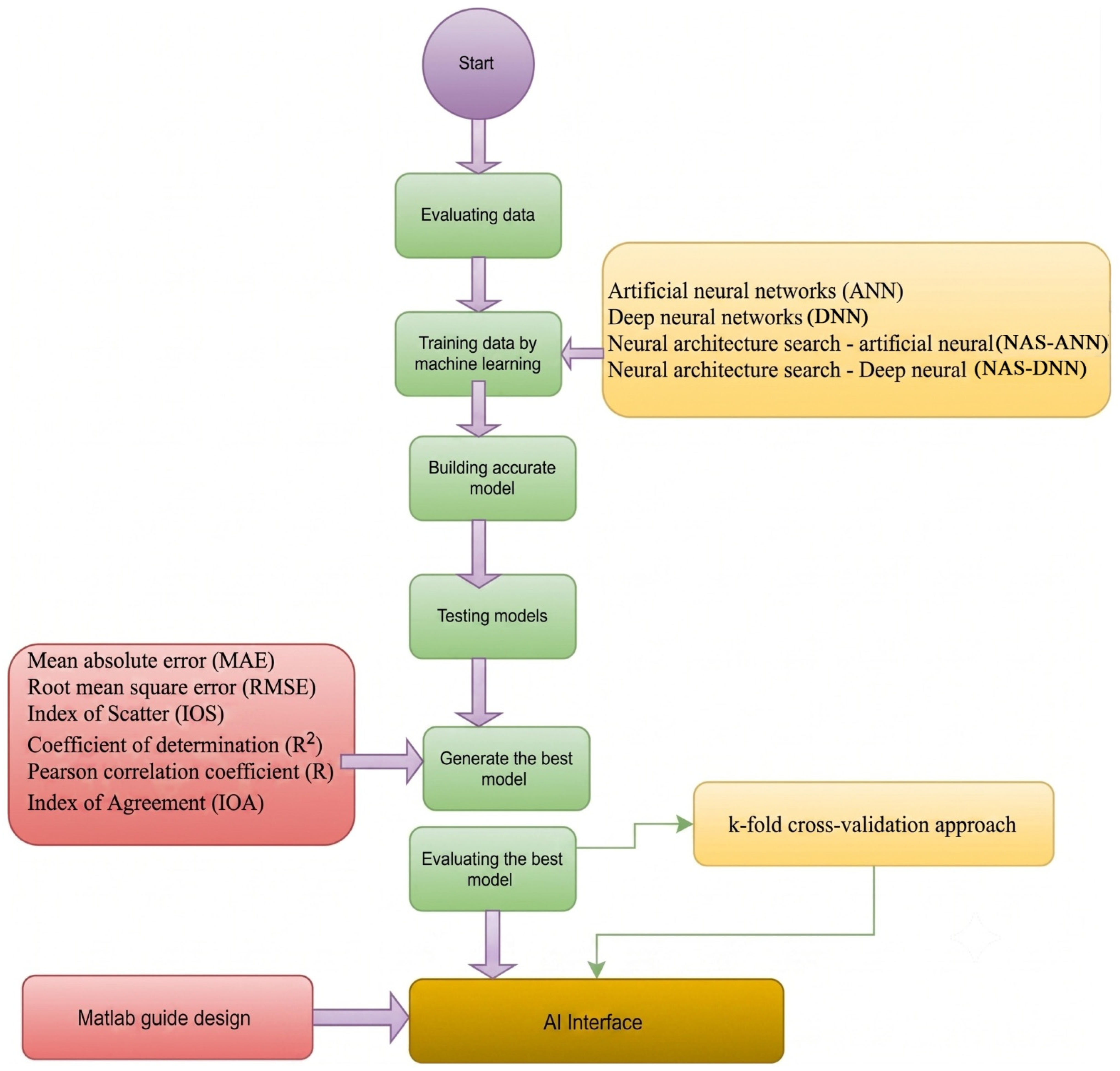
To provide a comprehensive operational blueprint of the predictive framework engineered in this study, the integrated data-driven process is systematically structured into four sequential, highly interconnected phases. The explicit technical execution path—progressing from raw multi-source field data curation to automated optimization, statistical validation, and deployment—is dynamically mapped out in the general methodology flowchart (Figure 2).

Phase 1: Multi-Source Data Curation: The baseline infrastructure of the model is built upon the consolidation of 1984 field sample records (comprising both cored and penetration strata) compiled from the coastal zone of Boumerdes. Prior to network injection, data cleaning and uniform Z-score normalization were executed solely on the training data to synchronize the disparate physical scales of the geotechnical input variables. This prevents the mathematical dominance of larger coefficients during backpropagation, justifying the use of Z-score normalization over standard Min-Max scaling, which fails by clamping highly skewed variables tightly to zero and compressing the main distribution, as reported in the literature [71].

Phase 2: Automated Architecture Optimization: To eliminate human-induced heuristic biases, the preprocessed datasets are routed into an Automated Machine Learning (AutoML) engine driven by Neural Architecture Search (NAS). The NAS algorithm systematically explores a predefined multi-dimensional structural search space to optimize the stacked hidden layer depth ($H$), internal node configurations ($N_1,N_2$), and non-linear transfer function combinations for both shallow and deep architectures (NAS-ANN and NAS-DNN). The ANN, DNN, NAS-ANN, and NAS-DNN models were implemented in MATLAB R2016a (MathWorks, Natick, MA, USA) using the Neural Network Toolbox provided in MATLAB R2015a. The networks were trained using the Levenberg–Marquardt backpropagation algorithm (trainlm) with the mean squared error (MSE) as the performance function. The hidden layers employed the hyperbolic tangent sigmoid activation function (tansig), whereas the output layer used the linear activation function (purelin). Input and output data were normalized using the mapminmax function before training and reverse-transformed after prediction. The dataset was randomly divided using the divider and function into 80% for training (1587 samples) and 20% for validation (397 samples), with no independent test set. Training was stopped automatically using an early stopping criterion (after 50 epochs of no improvement in validation loss) to prevent overfitting.

Phase 3: Multi-Criteria Statistical Verification: To ensure strong model generalization and explicitly mitigate hidden overfitting or underfitting risks, a stratified 5-fold cross-validation protocol ($K=5$) is nested directly within the training loops. Candidate architectures are rigorously scored against an advanced matrix of multi-criteria performance indicators—specifically tracking the simultaneous minimization of $MAE$, $RMSE$, and $IOS$, balanced against the optimization of $R^2$, $R$, and $IOA$ response boundaries.

Phase 4: Practical GUI Deployment: Following statistical verification, the optimized deep learning architecture is integrated into a standalone, interactive software application designated as GeoLiquefy-AI (v1.0). This engineered graphical user interface allows practicing geotechnical engineers to conduct rapid, non-programmer, on-site Factor of Safety ($F_s$) estimations, successfully bridging the gap between high-dimensional AI and sustainable urban hazard management.

3. Results

A comprehensive multi-source dataset consisting of 1984 soil samples was assembled to investigate the non-linear macro-spatial relationships between physically interpretable geotechnical/seismic parameters and the targeted Factor of Safety ($F_s$) against liquefaction. The dataset incorporated ten key variables: depth ($z$), lithology, wet density (${\gamma }_h$), water content ($w$), degree of saturation ($S_r$), fines content ($FC$), total overburden stress (${\sigma }_v$), effective overburden stress (${\sigma }_v^{\prime }$), cyclic stress ratio ($CSR$), and normalized peak ground acceleration ($a_{max}/g$).

3.1. Statistical Distribution and Exploratory Data Analysis

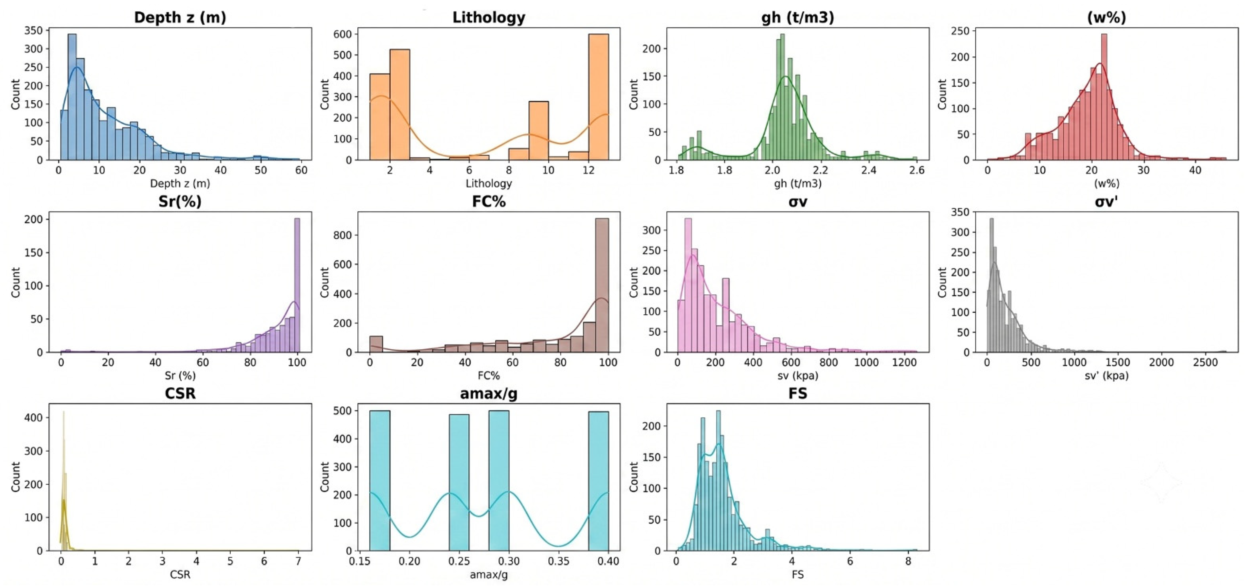
The statistical summary of the 1984 subsurface samples (

Table 4. Descriptive statistics of the multi-source geotechnical and seismic samples (n = 1984).

Parameter	Mean	Median	Min	25%	50%	75%	Max	Standard Deviation	Variance	Skewness	Kurtosis
Z (m)	11.674	8.475	0.55	4.5	8.475	16.5	59.5	9.841	96.85	1.773	4.097
lithology	6.625	8	1	2	8	13	13	5.107	26.077	0.146	−1.755
ϒh (t/m3)	2.046	2.06	1.61	2.01	2.06	2.11	2.6	0.155	0.024	−0.489	1.906
W(%)	19.296	20	5.3	16	20	22.62	45.96	5.752	33.089	0.233	1.96
Sr(%)	90.645	95.09	0	87	95.09	100	100	13.96	194.874	−3.457	16.612
FC%	78.419	93.14	5.95	65	93.14	98.32	100	28.086	788.834	−1.468	1.21
σv (kpa)	216.966	152.305	9.13	77.43	152.305	287.96	1267.4	196.975	38,799.1	2.138	6.116
σv′ (kpa)	219.69	150.975	9.13	76.5	150.975	288.14	2737.1	227.018	51,537.3	4.108	32.684
CSR	0.133	0.1	0	0.09	0.1	0.17	7.05	0.187	0.035	27.449	962.49
amax/g	0.275	0.3	0.16	0.16	0.3	0.4	0.4	0.088	0.008	0.144	−1.218
FS	1.628	1.48	0.11	1.02	1.48	1.842	8.31	0.88	0.774	2.252	8.323

) and the corresponding histograms (Figure 3) reveal a highly heterogeneous database, which is typical for coastal Quaternary deposits. By examining each variable in sequence, we can identify not only the central tendencies and spreads but also several anomalies that require careful interpretation.

• Depth (z) ranged from 0.55 m to 59.5 m, with a mean of 11.67 m and a median of 8.48 m. The positive skewness (1.773) and high kurtosis (4.097) indicate a right-tailed distribution: most boreholes are shallow to intermediate (0–20 m), while a few deep samples extend the tail to 60 m. No true anomaly was observed here. The skewness simply reflects the typical exploration practice where shallow investigation dominates over deep drilling.
• Lithology codes (1–13) presented a mean of 6.63, a median of 8, and a skewness near zero (0.146), suggesting a roughly symmetric distribution. The negative kurtosis (−1.755) indicates a flatter shape than the normal distribution, meaning that several facies codes (e.g., 8 and 13) appear with similar frequency. No statistical anomaly was detected, but the discrete nature of this categorical variable inherently produced a multimodal histogram.
• Wet density (γh) varied from 1.61 to 2.60 t/m³, averaging 2.05 t/m³. The slightly negative skew (−0.489) and moderate kurtosis (1.906) point to a nearly symmetric distribution with a gentle left tail. No anomaly was present; the few low-density values (down to 1.61) correspond to very loose organic-rich or highly porous sandy layers, which are physically plausible.
• Water content (w) ranged from 5.3% to 45.96%, with a mean of 19.3% and a median of 20%. The low skewness (0.233) and kurtosis (1.96) indicate a distribution close to normal, centered between 15% and 25%. The minimum of 5.3% is physically plausible for relatively dry surface soils or shallow samples above the water table. The distribution is well-behaved and requires no special treatment.
• Degree of saturation (Sr) ranged from 0% to 100%, with a mean of 90.6% and a median of 95.1%. The extreme negative skew (−3.457) and very high kurtosis (16.61) indicate that the vast majority of samples are nearly or fully saturated (concentrated between 95% and 100%), while a small number of drier samples create a long left tail extending down to 0%. The maximum value of 100% is physically plausible and does not represent an anomaly. However, the extremely high kurtosis (leptokurtic shape) reflects a very sharp peak near 100%, meaning that most soils in the coastal zone are fully saturated—which is geotechnically consistent with a shallow water table.
• Fines content (FC) ranged from 5.95% to 100%, with a mean of 78.4% and a median of 93.1%. The negative skew (−1.468) and the histogram’s massive peak near 100% indicate that the majority of soils are fine-grained (silts and clays). The minimum of 5.95% is physically plausible and corresponds to sandy soils with a small fraction of fines. No anomaly existed in this variable. The distribution simply reflects the dominance of fine-grained coastal alluvial deposits. Therefore, no corrective action is required for FC.
• Total overburden stress (σ_v) ranged from 9.13 to 1267 kPa, with a mean of 217 kPa and a median of 152 kPa. Effective overburden stress (σ′_v) ranged from 9.13 to 2737 kPa, with a mean of 220 kPa and a median of 151 kPa. The positive skewness (2.138 for σv, 4.108 for σ′v) and high kurtosis (6.12 and 32.68, respectively) indicate that the distributions are strongly concentrated at lower stress levels. As clearly visible in the histograms, the overwhelming majority of samples fall below 600 kPa for σv and below 500 kPa for σ′v, with only a very small number of higher values extending the tails. This pattern is physically consistent with the predominantly shallow to intermediate depths (most samples <30 m) and the presence of a shallow water table that reduces effective stresses.
• Cyclic Stress Ratio (CSR) ranged from 0.00 to 7.05, with a mean of 0.133 and a median of 0.10. The extreme positive skewness (27.45) and very high kurtosis (962.5) reflect a distribution where the vast majority of values are concentrated near zero (below 0.5), while a very small number of samples reach much higher values up to 7.05. This pattern is not unexpected given the physical definition of CSR. Since most boreholes are located at shallow to intermediate depths with moderate total and effective stresses, and the peak ground acceleration ratios are limited to 0.16–0.40, the computed CSR naturally remains low for the majority of records. The few high CSR values arise from unusual combinations of deeper depths, higher effective stresses, or possibly localized seismic amplification factors.
• Normalised acceleration (amax/g) ranged from 0.16 to 0.40, with no anomalies. The distribution is nearly uniform, with three peaks corresponding to the design PGA values (0.16, 0.30, 0.40) used in the study area. The negative kurtosis (−1.218) confirms a platykurtic shape.
• Factor of Safety (Fs) varied from 0.11 to 8.31, with a mean of 1.63 and a median of 1.48. The positive skew (2.252) and high kurtosis (8.323) reflect a concentration of values near the liquefaction threshold (Fs ≈ 1–2) and a long tail toward high safety factors. The maximum of 8.31 is unusual, but not impossible for very shallow, dense, dry soils under low seismic demand.

Overall, the descriptive statistics and histograms confirm the expected heterogeneity of the coastal geotechnical dataset. Prior to model training, the database was preprocessed using the Interquartile Range (IQR) method to detect and handle outliers, and K-Nearest Neighbors (KNN) imputation to replace missing values. This ensures that the NAS-DNN framework learns physically consistent relationships without distortion from anomalous entries.

3.2. Feature Interdependence and Correlation Analysis

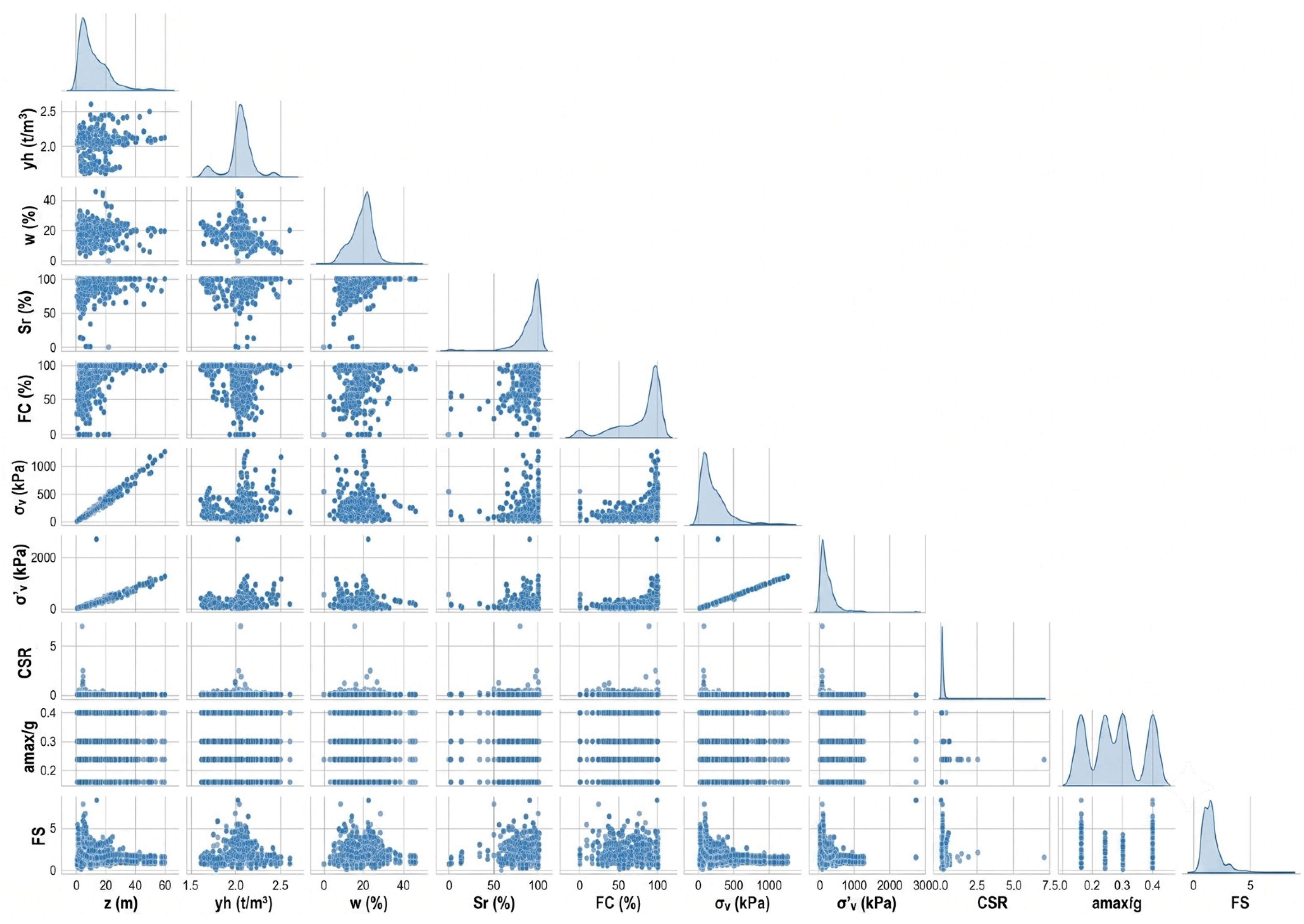
To further examine the linear interdependence between variables, a Pearson correlation analysis was conducted to quantify the strength and direction of the relationships between the predictive input parameters and the target Factor of Safety ($F_s$). Figure 4 presents the scatter plot matrix (pairplot) of all the variables, where the diagonal shows the histogram of each parameter, and the off-diagonal plots display the pairwise scatter distributions. This visual inspection complements the numerical correlations and reveals the general absence of clear linear trends, especially between $F_s$ and most predictors.

Overall, the correlation matrix (

Table 5. Pearson correlation matrix highlighting the linear relationships between geotechnical parameters.

	Z (m)	ϒh (t/m3)	W(%)	Sr(%)	FC%	σv (kpa)	σv′ (kpa)	CSR	amax/g	FS
Z (m)	1	0.132654	−0.00952	0.134144	0.318236	0.985881	0.857981	−0.17717	−0.0016	−0.15387
ϒh (t/m3)	0.132654	1	−0.3642	0.020295	−0.09268	0.152853	0.121419	−0.01375	−0.00385	0.002575
W(%)	−0.00952	−0.3642	1	0.471789	0.180665	−0.0992	−0.07476	−0.00985	−0.00123	−0.05437
Sr(%)	0.134144	0.020295	0.471789	1	0.301254	0.101384	0.082715	−0.04417	−0.00301	−0.11603
FC%	0.318236	−0.09268	0.180665	0.301254	1	0.310387	0.283306	−0.05584	−0.00139	−0.13948
σv (kpa)	0.985881	0.152853	−0.0992	0.101384	0.310387	1	0.871801	−0.17241	−0.0017	−0.16016
σv′ (kpa)	0.857981	0.121419	−0.07476	0.082715	0.283306	0.871801	1	−0.16507	−0.00149	−0.05406
CSR	−0.17717	−0.01375	−0.00985	−0.04417	−0.05584	−0.17241	−0.16507	1	−0.01609	−0.00804
amax/g	−0.0016	−0.00385	−0.00123	−0.00301	−0.00139	−0.0017	−0.00149	−0.01609	1	−0.01653
FS	−0.15387	0.002575	−0.05437	−0.11603	−0.13948	−0.16016	−0.05406	−0.00804	−0.01653	1

) highlights weak to moderate linear relationships among most input variables, indicating that the dataset is multidimensional and that conventional empirical models may not adequately capture these complex relationships. A strong positive correlation was observed between depth ($z$) and both total overburden stress (${\sigma }_v$) and effective overburden stress (${\sigma }_v^{\prime }$), with correlation coefficients of 0.986 and 0.858, respectively. This is physically consistent, as confining stresses increase with depth due to overburden consolidation. The fines content ($FC$) shows moderate positive correlations with depth (0.318), ${\sigma }_v$ (0.310), and ${\sigma }_v^{\prime }$ (0.283), suggesting an indirect relationship controlled by coastal stratigraphic variations where deeper layers tend to contain more fine particles.

Regarding the seismic loading parameters, the cyclic stress ratio ($CSR$) exhibited generally weak negative correlations with most geotechnical variables, particularly with ${\sigma }_v$ (−0.172) and ${\sigma }_v^{\prime }$ (−0.165). This reflects its distinct role as an external seismic demand parameter that is largely independent of the static soil properties. The normalized peak ground acceleration ($a_{max}/g$) showed negligible correlations with all the other variables (all values near zero), as expected because it is an independent seismic input.

Finally, the target output, Factor of Safety ($F_s$), exhibited weak to moderate negative correlations with most predictors. The strongest negative correlations were observed with ${\sigma }_v$ (−0.160), $FC$ (−0.139), and $S_r$ (−0.116). This trend is geomechanically consistent: increasing vertical stresses, higher fines content, and higher degrees of saturation all tend to reduce the granular soil’s resistance against liquefaction, thereby lowering the safety factor. The weak correlation magnitudes (mostly below 0.2 in absolute value) confirm that $F_s$ is governed by a complex, non-linear combination of multiple factors rather than by any single dominant predictor. The scatter plot matrix in Figure 4 further supports this observation, as no clear linear cloud is visible between $F_s$ and any individual input.

3.3. Algorithm Benchmarking and Predictive Performance

The core predictive capabilities of the evaluated computational models—baseline Artificial Neural Network (ANN), standard Deep Neural Network (DNN), and their automated Neural Architecture Search (NAS)-optimized variants (NAS-ANN and NAS-DNN)—were rigorously quantified using a comprehensive set of statistical performance metrics, as summarised in

Table 6. Performance evaluation metrics of the executed AI models for predicting liquefaction Factor of Safety (Fs).

Data Split	IA Method	R	R2	RMSE	MAE	IOS	IOA
Training	ANN	0.7053	0.497	0.636	0.375	0.382	0.804
	DNN	0.7497	0.5618	0.5851	0.3182	0.4700	0.8389
	NAS ANN	0.8853	0.7838	0.4133	0.2488	0.2521	0.9363
	NAS DNN	0.9518	0.9060	0.2772	0.1806	0.1700	0.9747
Validation	ANN	0.6508	0.4192	0.6149	0.3676	0.3537	0.7755
	DNN	0.7199	0.5034	0.6071	0.3441	0.4197	0.8677
	NAS ANN	0.8336	0.6949	0.4653	0.3056	0.2939	0.9083
	NAS DNN	0.8843	0.7819	0.3707	0.1741	0.2288	0.9388
ALL	ANN	0.6961	0.4846	0.6314	0.3731	0.4600	0.8387
	DNN	0.7421	0.5506	0.5896	0.3234	0.3071	0.7697
	NAS ANN	0.8760	0.7674	0.4242	0.2602	0.2606	0.9313
	NAS DNN	0.9409	0.8812	0.2832	0.1793	0.1818	0.9668

.

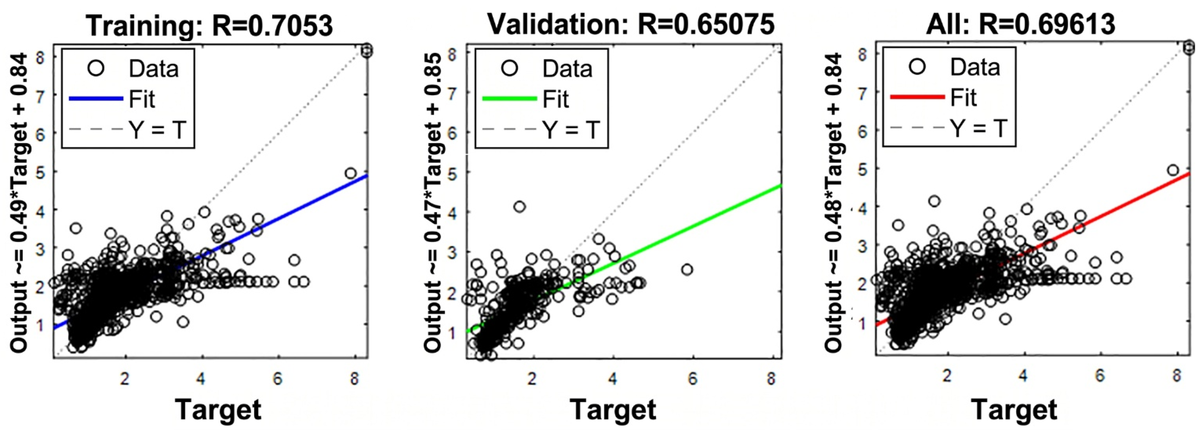
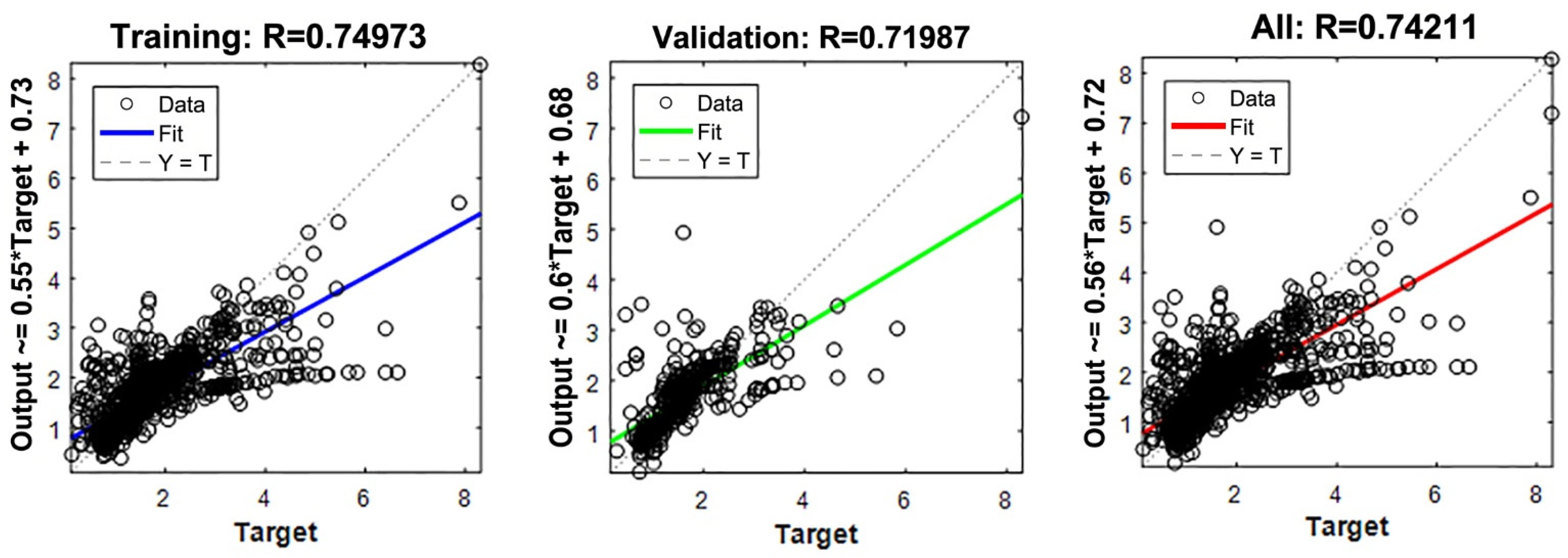
The traditional ANN architecture exhibited moderate predictive accuracy across all the phases. During training, it achieved an R of 0.7053, which dropped to 0.6508 on validation and yielded an overall (All) R of 0.6961. The corresponding All-phase RMSE and MAE were 0.6314 and 0.3731, respectively, while the Index of Agreement (IOA) remained 0.8387. The DNN model, with one additional hidden layer, showed a clear improvement over the shallow ANN: its training R reached 0.7497, validation R was 0.7199, and overall R rose to 0.7421. The global error metrics were also reduced (All RMSE = 0.5896, All MAE = 0.3234). However, both conventional networks suffered from a noticeable drop in performance when moving from training to validation (e.g., ANN R decreased by 0.0545, DNN by 0.0298), indicating limited generalization capacity despite their deeper architecture.

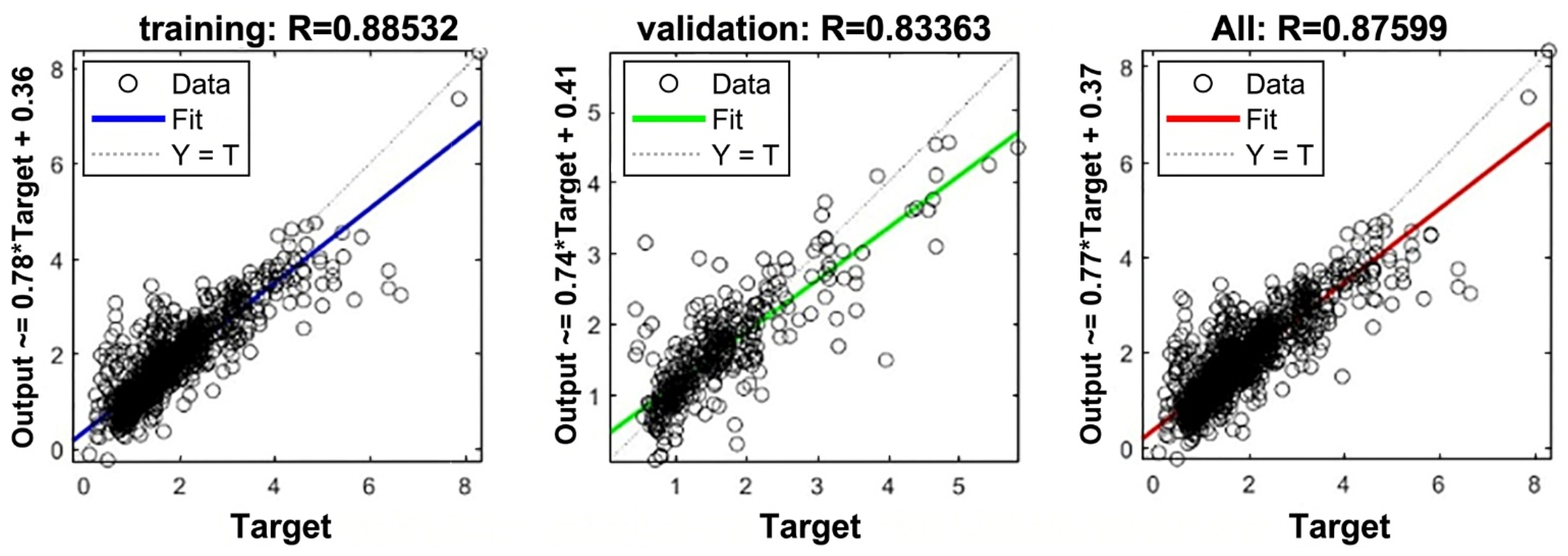
The integration of the Neural Architecture Search engine drastically minimized error parameters while maximizing structural agreement. The NAS-ANN model, which automatically optimizes the first hidden layer configuration (H = 1, N₁ ∈ [1–20]), yielded substantially higher correlations: training R = 0.8853, validation R = 0.8336, and overall R = 0.8760. Its overall RMSE (0.4242) and MAE (0.2602) were nearly 30% lower than those of the manually tuned DNN. Nevertheless, the most significant performance improvement was observed in the NAS-DNN variant, which explores deeper topologies (H = 1 or 2, N₁, N₂ ∈ [1–20], and activation functions). The NAS-DNN architecture configured the optimal model within the investigated search space, attaining an overall R of 0.9400, R² of 0.8812, and an IOA of 0.9668—demonstrating a high degree of statistical alignment between the observed and predicted Factor of Safety (F_s). Furthermore, it recorded the lowest global residual errors (RMSE_all = 0.2832, MAE_all = 0.1793), proving its exceptional capacity to map highly abstract, non-linear subsurface features.

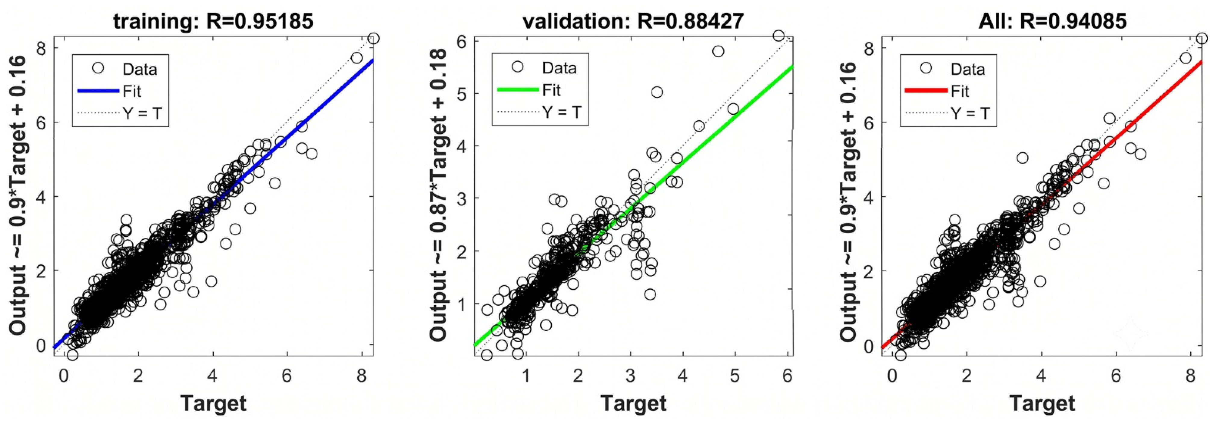
Graphical scatter-plot validations (Figure 5, Figure 6, Figure 7 and Figure 8) visually corroborate these statistical findings. Figure 5 shows the NAS-DNN predictions tightly converging around the ideal Y = T fit line, with minimal dispersion and a regression slope of approximately 0.94. Figure 6 (NAS-ANN) displays a broader scatter but still a clear positive correlation. Figure 7 and Figure 8 exhibit progressively larger deviations from the Y = T line, particularly at higher Fs values (>4), confirming the superiority of the automated search-driven topologies (where Figure 7 represents the standard DNN and Figure 8 represents the standard ANN).

3.4. Robustness Verification via Stratified K-Fold Cross-Validation

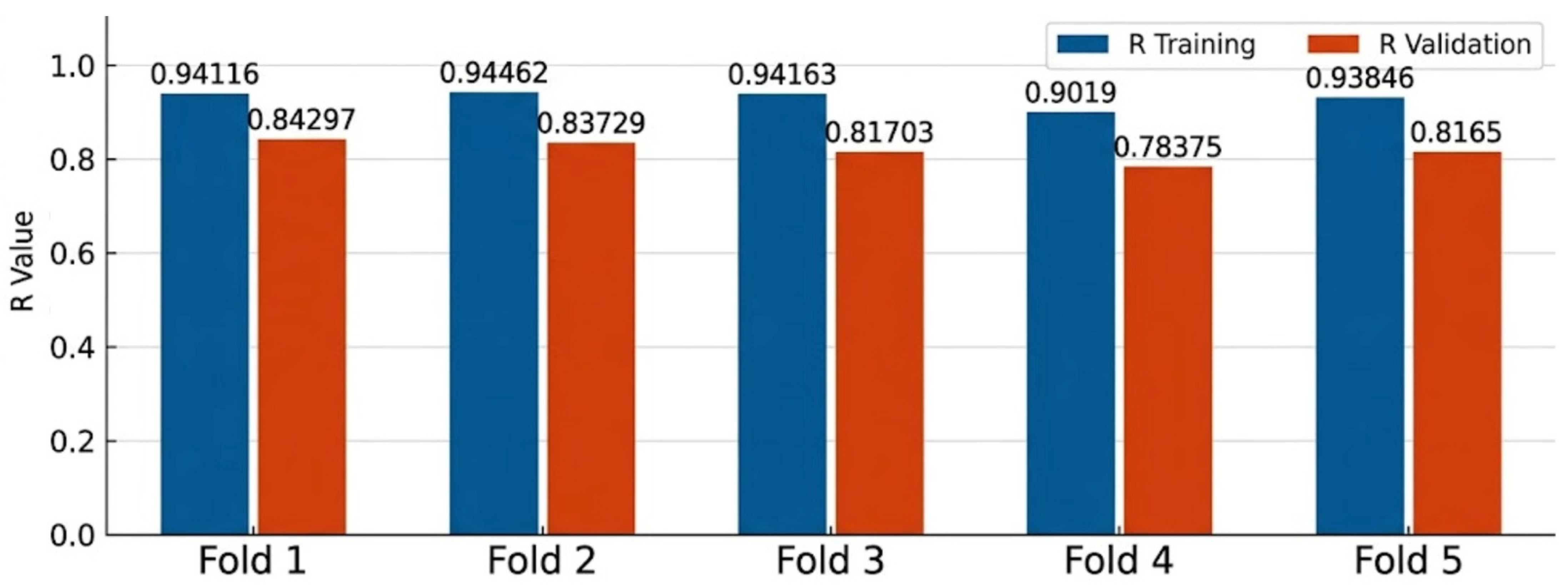
To rigorously eliminate any localized training bias and empirically confirm the spatial generalization capability of the chosen NAS-DNN model, a stratified 5-fold cross-validation procedure was executed. The dataset was randomly partitioned into five mutually exclusive folds, each preserving the original distribution of the target variable ($F_s$). In each iteration, four folds were used for training and the remaining fold for validation, and the process was repeated until every fold served once as the validation set. The resulting training and validation Pearson correlation coefficients ($R$) for each fold are summarised in Figure 9 (and the accompanying table).

The dynamic results indicate that the NAS-DNN architecture consistently maintains exceptional predictive accuracy across all five iterations. Training $R$ values ranged from 0.902 to 0.945, with a mean of approximately 0.933, while validation $R$ values lay between 0.784 and 0.843 (mean ≈ 0.819). Although a moderate drop between training and validation performance was observed (typical for any data-driven model), the validation correlations remained very high (all > 0.78). Notably, the smallest validation $R$ (0.78375, Fold 4) is still considered excellent for a highly heterogeneous geotechnical database. The minimal structural degradation across folds confirms that the NAS-DNN architecture is highly stable and immune to hidden overfitting or underfitting phenomena. No single fold dominates the error metrics, proving that the model’s predictive power is not an artefact of a particular data split.

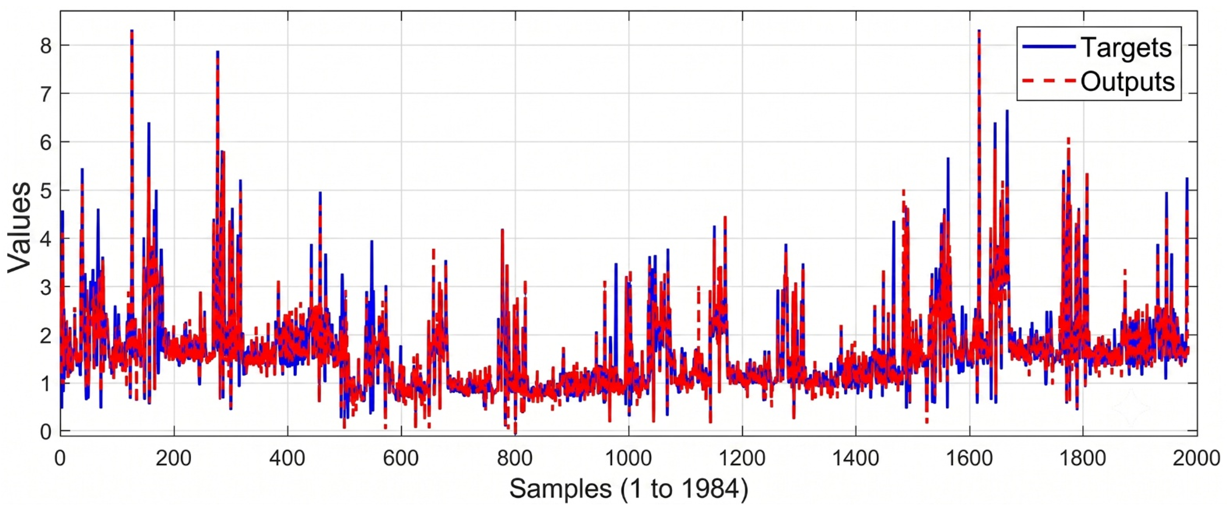
Furthermore, to assess the model’s ability to capture fine-scale variations and extreme events, the optimized NAS-DNN was applied to an independent test dataset. Figure 10 presents a comparative line plot of observed (target) versus predicted outputs for the entire test dataset. The model effectively captured sudden peaks (e.g., at sample indices where $F_s$ drops sharply) and extreme stratigraphic fluctuations, such as very low or very high safety factors. The predicted curve closely followed the observed target line, with only minor deviations in a few localized intervals. This visual corroboration, together with the consistently high cross-validation $R$ values, demonstrates that the NAS-DNN provides reliable out-of-sample predictions across the entire database, making it highly suitable for operational deployment in heterogeneous coastal environments.

3.5. Comparative Benchmarking with Existing Literature

To contextualise the scientific contribution of the proposed AutoML framework,

Table 7. Methodological benchmarking of the proposed NAS-DNN framework against existing AI-based liquefaction models.

References	Model Used	Samples	Correlation
[51]	SVM	134	89%
[52]	XGB, GBM, RF, SVR, and GMDH	620	79.91%
[53]	SVM, RF, and XGB	415	92.44%
[54]	DNN	556	93%
[55]	BP, SVM, DT, and KNN	620	92.3%
[56]	ANN-ABC, ANN-TLBO, ANN-ALO, ANN-ACO, ANN-ICA, and ANN-SCE	834	72.3%
[57]	DNN, CNN, LSTM, RNN, and BILSTM	834	90.6%
Our Study	ANN, DNN, NAS-ANN, and NAS- DNN	1984	94%

presents a comparative overview of the NAS-DNN approach against leading machine learning models in recent liquefaction literature. Previous studies have primarily employed diverse algorithms—such as SVM, RF, XGBoost, and various hybrid ANN architectures—to address liquefaction susceptibility assessment and probability of occurrence prediction. While these studies have established a robust baseline for seismic hazard screening, they typically operate within a classification-based task space, predicting categorical susceptibility or failure probability rather than continuous physical indices.

In this context, the proposed NAS-DNN framework focuses on the continuous prediction of the Factor of Safety ($F_s$). By training on a consolidated multi-source database of 1984 samples, the model achieved a correlation coefficient of $R=0.94$. We acknowledge that comparing performance metrics across different task spaces—such as binary susceptibility classification versus continuous $F_s$ regression—requires careful interpretation, as the underlying mathematical objectives and data requirements differ. Consequently, Table 7 should be viewed as a contextual benchmark of predictive performance within the broader domain of geotechnical liquefaction modeling. The results suggest that the integration of large-scale geotechnical data with Neural Architecture Search (NAS) offers a sophisticated automated pathway to map non-linear soil behaviors, effectively reducing the heuristic bias common in manual architecture tuning.

3.6. Model Interpretability and Feature Attribution via SHAP

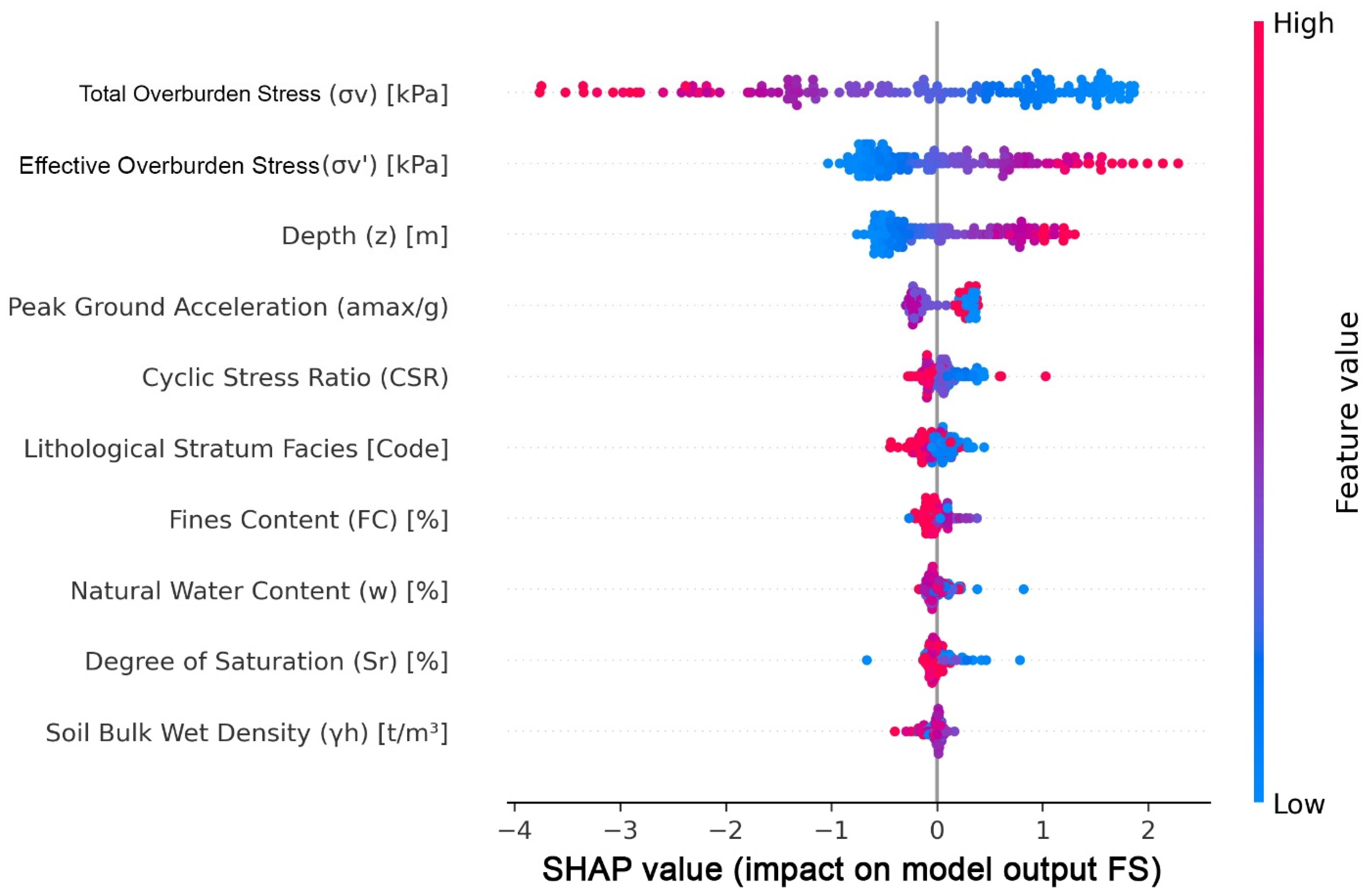
Figure 11 visualizes the global feature attribution and directional influence of the input parameters on the network’s predictive mechanics using the SHAP framework.

The SHAP distribution confirms that the network successfully captures fundamental soil mechanics principles rather than relying on arbitrary statistical mapping. Total overburden stress (${\sigma }_v$) emerges as the dominant governing feature; its high magnitudes (red data points) yield strongly negative SHAP values. This demonstrates the model’s physical understanding that a heavier total soil mass amplifies dynamic shear stresses during an earthquake, acting as a primary driving force that systematically reduces the Factor of Safety ($F_s$). Similarly, higher dynamic seismic demands—specifically $CSR$ and $a_{max}/g$—exhibit strongly negative impacts, accurately reflecting how increased seismic intensity drives soil failure.

Conversely, high effective overburden stresses (${{\sigma }_v}^{\prime }$) drive positive SHAP values, proving the network correctly learned that increased effective confining pressure acts as a resisting force, enhancing the cyclic shear strength and safety margin. Furthermore, fines content ($FC$) and depth ($z$) displayed a clustered impact near the neutral boundary, reflecting the highly non-linear threshold effects typical of silty sands. By transparently mapping these cross-correlations, the SHAP analysis validated the model’s geomechanical logic, establishing it as an auditable and trustworthy tool for regional seismic hazard screening.

3.7. Practical Deployment: The GeoLiquefy-AI Platform

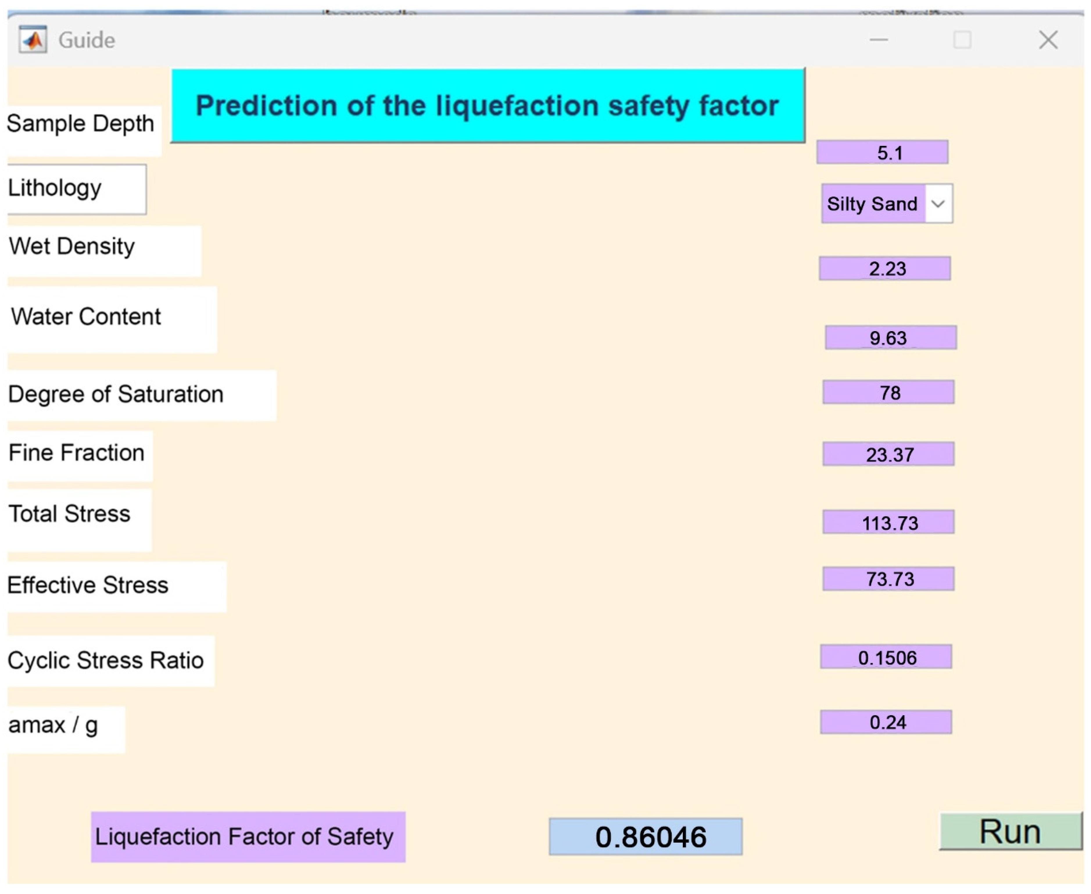
To bridge the persistent gap between high-dimensional academic modeling and immediate field engineering application, the optimized NAS-DNN mathematical architecture was successfully embedded into a standalone, interactive Graphical User Interface (GUI). Officially designated as GeoLiquefy-AI (v1.0), this intuitive digital platform allows practicing geotechnical engineers to instantaneously compute the site-specific liquefaction Factor of Safety ($F_s$) by simply inputting basic subsurface parameters.

As illustrated in Figure 12, the interface presents a user-friendly form containing all ten input variables required by the NAS-DNN model: depth ($z$), lithology (e.g., Silty Sand), wet density (${\gamma }_h$), water content ($w$), degree of saturation ($S_r$), fines content ($FC$), total stress (${\sigma }_v$), effective stress (${\sigma }_v^{\prime }$), cyclic stress ratio ($CSR$), and normalised peak acceleration ($a_{max}/g$). After the user enters the values (for instance, $z=5.1$ m, ${\gamma }_h=2.23$ t/m³, $w=9.63$%, $S_r=97$%, $FC=78$%, ${\sigma }_v=113.73$ kPa, ${\sigma }_v^{\prime }=73.73$ kPa, $CSR=0.1506$, $a_{max}/g=0.24$, and lithology selected as “Silty Sand”), clicking the Run button triggers the embedded NAS-DNN engine to compute the safety factor almost instantly—in this example, $F_s=0.86046$.

By bypassing the need for complex programming environments or manual recalculation of empirical formulas, this decision-support tool provides a highly efficient, deployment-ready solution for evaluating dynamic infrastructure safety. It also enables engineers to generate critical data layers for future macro-spatial hazard microzonation mapping, thereby accelerating risk-informed urban planning in seismically active coastal zones.

4. Discussion

4.1. Main Findings of the Present Study

The primary objective of this research was to engineer an automated, high-fidelity deep learning framework capable of decoding the complex, non-linear mechanics of earthquake-induced soil liquefaction in vulnerable coastal environments. The study systematically evaluated conventional Artificial Neural Networks (ANN) and Deep Neural Networks (DNN) against their automated, Neural Architecture Search-optimized counterparts (NAS-ANN and NAS-DNN) using a large regional dataset of 1984 geotechnical records from the Boumerdes coastal zone.

The analytical results clearly indicate that the hybrid NAS-DNN architecture represents the global mathematical optimum for predicting the liquefaction Factor of Safety ($F_s$). The model achieved high predictive fidelity, recording an overall Pearson correlation coefficient of $R=0.9400$, a coefficient of determination of $R^2=0.8812$, and an Index of Agreement (IOA) of 0.9668, whilst minimizing absolute residual errors (MAE = 0.1793, RMSE = 0.2832). Furthermore, stratified 5-fold cross-validation confirmed that the NAS-DNN structure is highly stable, preserving spatial generalization capabilities without succumbing to hidden overfitting phenomena (validation $R$ values consistently above 0.78 across all the folds). Finally, the research successfully transitioned these high-dimensional mathematical transformations into a deployment-ready decision-support tool via the GeoLiquefy-AI (v1.0) graphical user interface, enabling instantaneous, on-site hazard calculations for field engineers.

Beyond predictive performance, a post hoc SHAP analysis further validated the model’s robustness by confirming that the NAS-DNN architecture successfully mirrors fundamental soil mechanics; it identified total overburden stress (${\sigma }_v$) and seismic demand ($CSR$) as the primary drivers of liquefaction, while correctly recognizing the stabilizing influence of effective confining pressure (${{\sigma }_v}^{\prime }$), thereby establishing a transparent and geomechanically sound framework for field application.

4.2. Comparison with Other Studies

Situating these findings within the broader trajectory of computational geotechnics highlights the distinct structural advantages of the proposed methodology. A comprehensive benchmarking against recent predictive models—including Support Vector Machines [51], gradient boosting ensembles [56], and standard deep learning networks [54,57]—reveals a persistent performance ceiling in existing literature, typically hovering between 72% and 93% correlation (Table 7).

In contrast, the methodology deployed in this research transcends these barriers through four systematic advancements: first, by curating and rigorously preprocessing a comprehensive database of 1984 multi-source geotechnical records, the model achieves an important level of statistical robustness. Second, the integration of a hybrid AutoML-driven Neural Architecture Search (NAS) engine eliminates human-induced heuristic biases, allowing the architecture to mathematically optimize the deep neural topology to fit the non-linear soil degradation continuum. Third, the implementation of a stratified 5-fold cross-validation protocol ensures that the model maintains consistent predictive stability across heterogeneous strata, effectively neutralizing the overfitting risks that frequently compromise standard models in smaller datasets. Fourth and finally, while earlier studies focused on categorical classifications that simplify complex failure mechanics, the current research introduces a continuous regression framework coupled with an auditable SHAP-based feature attribution. By integrating this XAI framework, we provide transparent geomechanical validation that maps how seismic demand and confining pressure govern the Factor of Safety ($Fs$). This is further complemented by the development of the “GeoLiquefy-AI” graphical user interface, which bridges the gap between high-dimensional academic algorithms and field-scale engineering deployment.

4.3. Implication and Explanation of Findings

The exceptional predictive accuracy achieved by the NAS-DNN framework is deeply rooted in its capacity to autonomously map the physical mechanics of soil failure into an optimized algorithmic architecture. Coastal liquefaction is not governed by a single dominant parameter, but rather by the highly non-linear interaction of seismic demand ($CSR$, $a_{max}/g$), stratigraphic confinement (${\sigma }_v$, ${\sigma }_v^{\prime }$, depth), and hydro-mechanical soil states ($w$, $S_r$, $FC$). The hybrid NAS algorithm explicitly excels in this high-dimensional environment by iteratively engineering deep hierarchical hidden layers capable of extracting these abstract physical interdependencies.

From a practical engineering perspective, the implications of these findings are transformative. Although the proposed model uses the same fundamental geotechnical and seismic input parameters as conventional semi-empirical methods, its data-driven architecture is capable of learning complex nonlinear relationships and interactions among variables. This enables a more flexible representation of the heterogeneous behavior of Boumerdes soil and contributes to improved predictive performance within the investigated study area. The deployment of the GeoLiquefy-AI platform demonstrates that complex deep learning architectures can be distilled into an intuitive, real-time computational format. This operational shift implies that geotechnical engineers can now rapidly assess site-specific liquefaction potential without initiating computationally exhaustive finite element simulations, thereby accelerating the implementation of sustainable land-use and disaster mitigation strategies.

4.4. Strengths and Limitations

A defining strength of this research lies in its empirical foundation: the compilation of 1984 rigorously preprocessed spatial records establishes one of the largest and most reliable data matrices deployed in regional liquefaction studies. Coupled with the integration of an advanced AutoML NAS engine and rigorous 5-fold cross-validation, the methodology actively suppresses variance and bias, ensuring exceptional generalization within the studied coastal domain.

Notwithstanding these findings, certain methodological limitations must be acknowledged. The NAS-DNN architecture was trained exclusively on Quaternary sedimentary profiles from the northern tectonic margin of Algeria. Consequently, while the internal mathematical logic is fundamentally sound, direct application of the model to drastically different geological environments—such as highly gravelly soils, non-coastal stiff clays, or regions with distinct seismo-tectonic rupture mechanisms—may require domain adaptation or transfer learning to preserve optimal accuracy. Additionally, while the utilized parameters comprehensively capture the static and cyclic stress states, the current dataset does not directly ingest deep geophysical variables, such as continuous shear-wave velocity ($V_s$) profiles, which could further refine the mapping of localized site amplification effects. Furthermore, a key conceptual limitation of the current model must be noted regarding the assessment of liquefaction consequences. While GeoLiquefy-AI (v1.0) successfully predicts the free-field liquefaction Factor of Safety ($F_s$), it does not account for the specific vulnerability characteristics of the overlying infrastructure, such as foundation configurations, structural loads, or building stiffness. In geotechnical engineering practice, a comprehensive hazard assessment requires a performance-based design approach that couples soil triggering potential with building-specific responses. Finally, from a methodological validation perspective, the historical nature of our legacy dataset (1980s–present) introduced a constraint: many borehole records lack precise coordinates, which precluded the use of spatial cross-validation. Consequently, we implemented standard k-fold cross-validation. We acknowledge this as a limitation; future research using georeferenced databases should prioritize spatial validation strategies to further refine generalization estimates.

4.5. Recommendations and Future Directions

This study successfully bridges the critical gap between theoretical computational intelligence and applied macro-spatial environmental monitoring. The integration of Neural Architecture Search (NAS) with Deep Neural Networks significantly improves the predictive accuracy of soil liquefaction potential mapping, fundamentally outperforming conventional empirical and standard machine learning paradigms.

It is highly recommended that regional disaster management authorities and civil engineering regulatory bodies integrate data-driven interfaces, such as the GeoLiquefy-AI platform, into their preliminary site investigation protocols. Utilizing such tools will significantly optimize the allocation of exploratory resources, providing rapid hazard screening prior to heavy infrastructure development in vulnerable coastal zones.

Future research trajectories should focus on integrating this deep learning architecture directly into Geographic Information Systems (GIS) to generate dynamic, real-time 3D seismic hazard microzonation maps. Furthermore, expanding the optimization search space to ingest heterogeneous geophysical signals (e.g., $V_s$ mapping and H/V spectral ratios) and utilizing transfer learning protocols will be essential to scale this predictive framework for global applicability across diverse seismically active land systems.

5. Conclusions

This study successfully engineered a hybrid automated Artificial Intelligence framework to predict earthquake-induced soil liquefaction across the highly vulnerable coastal margin of Boumerdes, Algeria. By integrating an extensive, multi-source database of 1984 geotechnical records with an advanced Neural Architecture Search (NAS) engine, the research systematically overcame the computational limitations and heuristic biases inherent in conventional empirical and manual machine learning approaches. The principal conclusions derived from this investigation are outlined below.

• The optimized NAS-DNN architecture emerged as the most effective topology for modeling complex, non-linear seismic soil failure within the predefined search space. It demonstrated consistent predictive reliability, outperforming standard ANN, DNN, and NAS-ANN baseline models. The model achieved a training correlation coefficient ($R_{train}$) of 0.9518, a validation coefficient ($R_{validation}$) of 0.8843, and a mean cross-validated $R$ of approximately 0.82, while effectively minimizing absolute residual errors.
• The implementation of a stratified 5-fold cross-validation protocol empirically confirmed the model’s spatial generalization capability. The NAS-DNN maintained consistent predictive stability across heterogeneous Quaternary strata, effectively neutralizing the hidden overfitting risks that frequently compromise standard data-driven models.
• Furthermore, by integrating SHAP analysis, this study demystifies the NAS-DNN’s internal decision-making process, demonstrating that the model’s predictive mechanics are firmly rooted in established geomechanical principles. This transparency validates the network’s capacity to correctly attribute soil liquefaction potential to key drivers such as seismic demand and confining pressure, thereby transforming the deep learning framework from a predictive ‘black box’ into an auditable, physics-informed decision-support system suitable for critical geotechnical engineering audits.
• The development of the “GeoLiquefy-AI (v1.0)” graphical user interface successfully bridged the critical gap between high-dimensional academic algorithms and field engineering application. This deployment-ready decision-support platform enables rapid, on-site calculation of the liquefaction Factor of Safety ($F_s$), entirely bypassing the need for complex programming environments.
• The proposed automated deep learning framework provides a scalable, data-driven foundation for liquefaction potential assessment. By equipping geotechnical engineers with a reliable computational mechanism, this research establishes the necessary groundwork for future studies aimed at generating highly accurate seismic hazard microzonation maps for anthropogenically altered coastal terrains.

While this research leverages a robust dataset of 1984 records and an advanced AutoML framework to minimize predictive bias, its current application is confined to the specific geological formations of the Boumerdes coastal zone. Practitioners should be aware that the model’s reliability is tied to this local geomorphological context. Consequently, to enhance the model’s regional generalization and broaden its operational scope, future research must focus on expanding the database to include diverse liquefiable geological formations across other geographical areas.

Ultimately, the integration of Hybrid Automated Machine Learning (AutoML) with comprehensive subsurface databases offers a systematic framework for regional liquefaction susceptibility assessment. Future research trajectories must prioritize the ingestion of non-invasive continuous geophysical parameters (e.g., $V_s$ profiles) into the NAS space, and adapt these deep learning protocols within active Geographic Information Systems (GIS) to scale global seismic risk mitigation effectively.