Identifying Key Drivers of Heavy Metal(loid)s Contamination in Farmland Soils Using Machine Learning with Source-Integrated Features

Abstract

Accurate source identification is essential for the prevention and control of heavy metal(loid)s (HMs) contamination in farmland soils. Conventional source-apportionment approaches often rely on limited indicators and expert judgment, which can increase uncertainty in source interpretation. In this study, 800 topsoil samples collected from farmland in Ningxia, together with 24 environmental and anthropogenic variables, were used to develop element-specific machine learning models for Cd, Cr, Hg, Pb, and As. Five algorithms, including random forest (RF), Extra Trees (ET), extreme gradient boosting (XGBoost), light gradient boosting machine (LightGBM), and least absolute shrinkage and selection operator (LASSO-stacking), were compared, and Shapley additive explanations (SHAP) were used to interpret the variables statistically associated with the spatial variability of each metal. Positive matrix factorization (PMF) was further applied to identify potential source categories. Model performance varied among metals, indicating element-specific differences in predictability and controlling factors. SHAP analysis showed that precipitation, temperature, spatial coordinates (longitude/latitude), cropping intensity, and industrial-source fine particulate matter emissions were among the most important associated factors, although their relative importance differed across elements. PMF results suggested that 73.8% of Cd was associated with agricultural inputs, 87.6% of Hg with industrial atmospheric deposition, and 68.4% of Cr and 46.7% of As with natural sources, Pb showed relatively weak predictability, suggesting that its spatial variability may be influenced by unmeasured local or legacy inputs, while model-derived associations indicated possible links with spatial gradients, terrain-hydrological conditions, wind-related variables, and soil carrier properties. Overall, this study presents an integrated framework that combines machine learning-based associated-factor analysis with receptor-model source apportionment, providing a more nuanced understanding of HMs contamination in farmland soils and supporting targeted soil pollution prevention and control.

1. Introduction

Farmland soil pollution has emerged as a critical environmental issue, posing substantial risks to food security and human health worldwide [1,2]. Heavy metals and metal(loid)s are of particular concern due to their pronounced toxicity, bioaccumulative potential, and environmental persistence [3,4,5]. Once introduced into agricultural soils, these elements can be readily taken up by crops and subsequently enter the food chain (web), thereby posing long-term and often irreversible threats to ecosystem integrity and human well-being [6,7,8]. Therefore, the effective characterization and source identification of heavy metal(loid)s contamination in farmland soils would provide essential technical support for environmental science and sustainable agriculture, offering informative guidance for soil environmental management practices.

Classical source apportionment approaches for soil heavy metal(loid)s contamination are largely data-driven and rely on statistical or receptor-model-based predictions, such as multivariate statistical analyses, including principal component analysis (PCA), factor analysis (FA), and cluster analysis (CA); receptor models, including positive matrix factorization (PMF) and absolute principal component scores–multiple linear regression (APCS-MLR); and their combinations with spatial analysis. In addition, some studies attempt to evaluate pollution risks directly from the upstream sources by characterizing source-side “pollution potential” (e.g., industrial emission/risk potential) and integrating it with soil contamination risk to support source-oriented prevention and control [9]. Other studies conduct soil monitoring under assumed or “default” polluted backgrounds (e.g., near factories, mining areas, and roads/traffic corridors) to approximate the impacts of likely source categories on soil heavy metal(loid)s enrichment [10]. However, source apportionment based on these research designs often remains component-based classification or statistically inferred attribution, and its reliability can be constrained by strong spatial heterogeneity and model uncertainty in soils. International evidence supports the need to interpret metal contamination within region-specific environmental and source contexts. Alharbi reported that agricultural soils in arid Central Saudi Arabia require continuous monitoring to safeguard soil quality and food security [11]. Nour showed spatially heterogeneous metal accumulation in Egyptian sediments, reflecting redistribution processes [12]. At a broader scale, Hou mapped toxic-metal pollution in global croplands and emphasized climatic, topographic, and anthropogenic controls [1]. Similarly, Saha et al. (2024) identified mining and smelting as key sources of metal(loid) enrichment in semi-arid Mexican soils, supporting source-informed assessment [13].

Comparatively fewer studies explicitly build models that directly link contaminants to measurable source-contribution factors through distributional patterns (e.g., spatial differentiation drivers, distance-to-source effects, and pathway-specific decay), although recent work has begun to incorporate distance variables and spatial detector methods to strengthen such direct linkages. To systematically characterize the risk profiles of heavy metal(loid)s contamination in farmland soils, investigation and assessment of their spatial distributions are essential technical approaches [14,15]. Considering that soil heavy metal(loid)s monitoring is generally conducted at discrete sampling points [16,17,18], a comprehensive and area-wide characterization of their spatial patterns should be achieved through spatial simulation and prediction techniques. Existing studies have primarily relied on spatial interpolation methods [19,20], spatial statistical regression models [21,22], machine learning-based prediction approaches [23,24], process-based mechanistic models [25,26,27], and the integration and nesting of various functions or models in hybrid frameworks [28,29,30] to infer spatial distributions from limited observations of soil contamination. Among the above pollution mapping approaches, spatial interpolation methods originate from mining engineering and geostatistics [31,32], and rely primarily on spatial information and spatial autocorrelation as their core predictive variables. Spatial statistical regression models extend traditional regression frameworks by explicitly incorporating spatial dependence, enabling the quantification of relationships between soil heavy metal(loid)s levels and environmental or socioeconomic covariates [33,34]. Process-based mechanistic models simulate the transport, transformation, and accumulation of heavy metal(loid)s in soils by specifically representing physical, chemical, and biogeochemical processes, thereby providing mechanistic interpretability [35,36]. However, spatial interpolation methods have limited ability to capture complex the nonlinear relationships between soil heavy metal(loid)s and multiple categories of environmental determinants, and their predictive performance is often constrained by sparse sampling or pronounced spatial heterogeneity of soil contaminants [37,38]. Spatial regression models share similar limitations with traditional regression approaches, as they are typically restricted to linear or weakly nonlinear assumptions [39,40,41,42]. Process-based mechanistic models for predicting soil heavy metal(loid)s concentrations tend to be relatively specialized, which might be inappropriate for comprehensive pollution mapping.

Machine learning approaches can capture nonlinear relationships between soil heavy metal(loid)s and multiple environmental contributors under fewer prior assumptions, enabling more flexible prediction in heterogeneous and non-stationary environmental systems [43,44,45]. Because of their predictive performance and capacity to reveal complex associations, machine learning methods have been increasingly applied to environmental pollution assessment. Recent studies have combined receptor models with self-organizing maps (SOM), convolutional neural networks (CNN), GeoDetector, and related algorithms to support quantitative source apportionment and driver identification in regions affected by multiple pollution sources [46,47,48].

However, technical limitations and knowledge gaps remain. First, soil properties, topographic factors, and environmental–meteorological conditions are the primary covariates considered in existing machine learning-based predictions of soil heavy metal(loid)s contamination. Though human activities are also mentioned, the characterizing indicators, such as population density, light intensity, and gross domestic product (GDP), are often too generalized to effectively identify and model the potential contributions of anthropogenic sources to soil heavy metal(loid)s contamination [49,50,51]. Second, traditional single-machine learning models exhibit varying predictive accuracy across different feature–target relationships under multiple feature combination scenarios [52], limiting the accuracy and interpretability of simulations involving diverse and numerous features. The compounding and interactive effects of these two limitations further challenge the accurate identification and quantification of anthropogenic drivers—including agricultural, industrial, and residential activities—which are recognized as key contributors to heavy metal(loid)s contamination in farmland soils [53,54,55].

To address the above limitations, this study aims to develop a potential driver identification framework for farmland soil heavy metal(loid)s contamination based on a stacking machine learning ensemble and the integration of multisource, high-spatial-resolution feature data. Specifically, we first introduce predictive features that more effectively and spatially precisely characterize anthropogenic pollution, enabling a systematic and comprehensive representation of human influences on soil contamination within a unified analytical framework alongside other potential drivers, such as soil properties, natural conditions, and geographical factors. High-spatial-resolution emission inventories and environmental statistical data are innovatively translated and incorporated as primary inputs into soil contamination prediction, representing a substantial improvement over existing approaches that rely on semi-quantitative and indirect proxies to measure anthropogenic drivers. Second, we employ a multi-model stacking ensemble to mitigate performance disparities among individual models when handling heterogeneous feature types and distributions, thereby overcoming limitations in model generalizability and interpretability and improving the performance of farmland soil heavy metal(loid)s predictions. Collectively, these methodological advances increase the informational depth and feature breadth of soil contamination prediction and provide more intuitive insights into soil contamination risk from a source-contribution perspective. Ningxia Hui Autonomous Region, a typical agro–industrial–residential interlaced region, was selected as the case study area. The contributions of 42 features to five major farmland soil heavy metal(loid) contaminants were quantified, and their spatial pollution levels were predicted.

2. Methods and Materials

2.1. Study Area and Farmland Soil Sampling

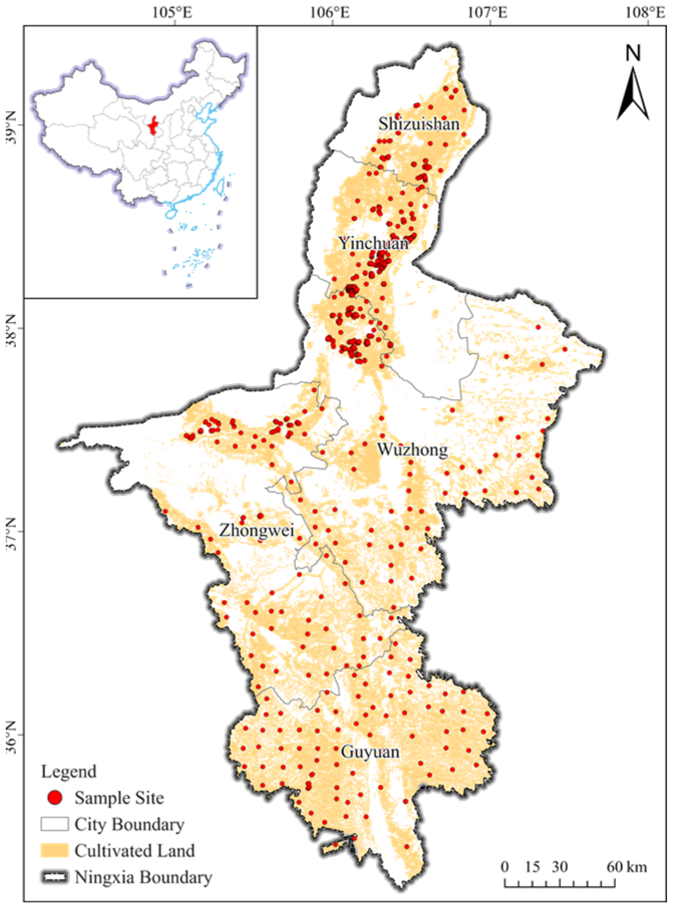
Ningxia is a provincial-level administrative region in western China, covering approximately 66,400 km² and located in the temperate continental arid and semi-arid climate zone of the upper Yellow River Basin [56,57]. It is also a national pilot zone for agricultural green development and an important energy-industry base in western China [58,59]. Farmland soil, covering 11,984.28 km², represents a vital production and ecological resource in this region and is influenced by complex interactions between natural and anthropogenic factors. Previous studies have shown that heavy metal(loid)s in Ningxia agricultural soils originate from multiple sources, including agriculture, industry, transportation, and residential activities [60,61]. Long-term changes in landscape patterns have also produced a fragmented configuration of farmland and other land-use types [62,63], further increasing the spatial heterogeneity and complexity of soil contamination and its potential drivers.

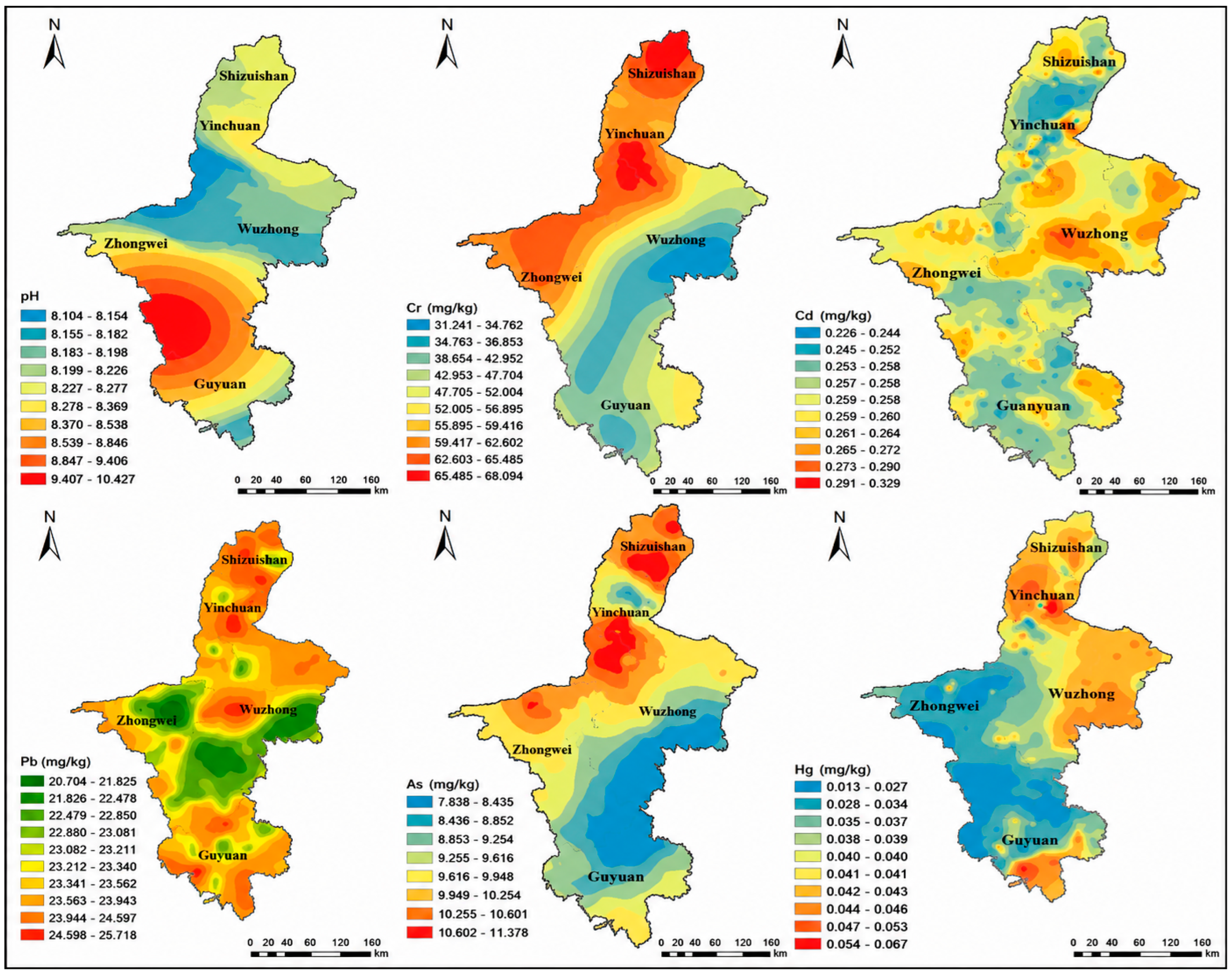
In 2024, this study conducted a sampling survey of five major heavy metal(loid)s, including total arsenic (As), mercury (Hg), cadmium (Cd), chromium (Cr), and lead (Pb), in agricultural soils across Ningxia. Guided by soil census, detailed survey, and routine monitoring data compiled by the Ningxia Department of Agriculture and Rural Affairs, we adopted a hybrid sampling design that combined systematic grid-based sampling with intensified sampling in priority areas, establishing 800 monitoring sites (0–20 cm) across the region (Figure 1 and Figure 2). The five heavy metal(loid)s are explicitly assigned risk intervention values in China’s national standard, Soil Environmental Quality—Risk Control Standard for Soil Contamination of Agricultural Land (GB 15618–2018) [64], highlighting their potential threats to the safety of agricultural products and human health. Although this standard provides a consistent basis for identifying areas of potential regulatory concern, it may not fully capture local ecological sensitivities within Ningxia. Soil pH, organic matter, texture, geochemical background, irrigation practices, crop types, metal bioavailability, and crop uptake can all influence the actual environmental and food-safety risks associated with heavy metal(loid) contamination. Therefore, the risk interpretation in this study should be regarded as a screening-level assessment, and future work should integrate national standards with locally calibrated ecological sensitivity and crop-uptake information. They have also been identified as the dominant soil contaminants, according to research based on China’s national soil quality survey. Therefore, this study selected the five heavy metal(loid)s as the target variables for the machine learning-based driver identification of farmland soil heavy metal(loid)s.

2.2. Model Establishment

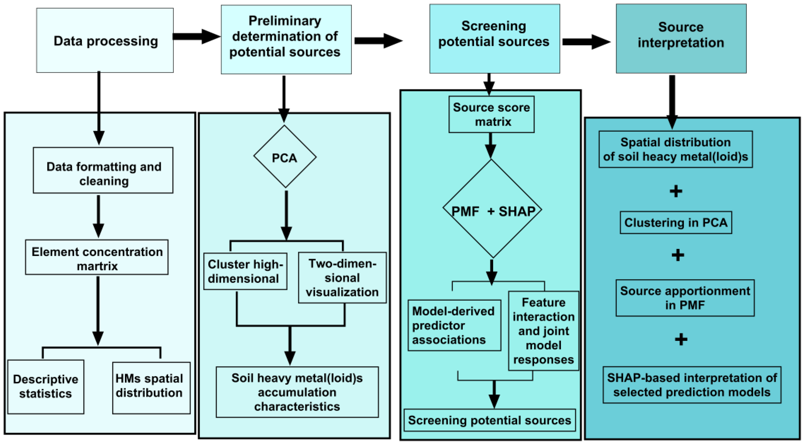
Figure 3 summarizes the overall analytical workflow, including data preprocessing, preliminary source identification by PCA, source screening through PMF and SHAP-based driver interpretation, and final source interpretation by integrating heavy metal(loid) spatial distributions, PCA clustering, PMF apportionment, and Least Absolute Shrinkage and Selection Operator (LASSO)-stacking ensemble framework.

Based on farmland soil sampling data, this study develops a, where LASSO regression serves as the meta-learner, to integrate predictions from multiple machine learning models. The LASSO-stacking framework leverages the strengths of different models in fitting and trend characterization, reducing reliance on any one model structure [65,66]. Before machine learning modeling, the initial set of candidate variables was subjected to multicollinearity screening using the variance inflation factor (VIF). Variables with VIF values < 5 were retained for subsequent analysis. This procedure was used to minimize redundancy among predictors and to improve the robustness of model fitting and SHAP interpretation. The retained variables covered multiple dimensions, including spatial location, climate, topography, soil properties, vegetation, population, cropping intensity, and emission-related factors, and all satisfied the predefined collinearity threshold. This approach provides improved generalizability, interpretability, and robustness, while enhancing spatial predictive performance in the context of soil heavy metal(loid)s contamination—a complex environmental issue driven by multiple interacting factors. Specifically, using 24 feature variables representing natural–environmental conditions and human activities, multiple base learners are constructed to capture the nonlinear relationships between heavy metal(loid)s concentrations and multi-classification factors. Driver factor identification by these base models is subsequently combined through the LASSO-stacking approach. On this basis, Shapley additive explanations (SHAP), an interpretability framework grounded in cooperative game theory, are applied to quantitatively assess the relative contributions of individual features to the model predictions [67,68,69], depicting the influences of potential drivers to heavy metal(loid)s contamination in farmland soils.

Within the LASSO-stacking ensemble, four complementary base learners were selected: random forest (RF), extreme gradient boosting (XGBoost), extremely randomized trees (ET), and light gradient boosting machine (LightGBM). These algorithms were chosen to capture relationships and interactions between feature and target variables from distinct modeling perspectives [70,71,72]. Base-model selection was guided by predictive capability and model diversity, ensuring that each learner contributed unique information to the ensemble. LASSO-stacking regression was then used as the meta-learner to derive an optimal weighted combination of base-model predictions [73,74]. Prediction outputs from the base learners were generated through cross-validation and entered into the meta-model, promoting a parsimonious ensemble structure.

The uncertainty and stability of the PMF solution were further evaluated using bootstrap analysis with 200 resampling runs. Bootstrap factor profiles were matched to the base-run factors according to their correlation and interpretability. Factor mapping rates, median profiles, and confidence intervals were used to assess the reproducibility of the source factors. In addition, DISP was conducted to evaluate rotational ambiguity and factor swapping. The final source apportionment results were interpreted only when the factor profiles were stable, environmentally meaningful, and consistent across validation diagnostics. To assess the robustness of SHAP-based feature rankings, a bootstrap stability analysis was performed. Specifically, the training dataset was resampled with replacement for 100 iterations. In each iteration, the complete modeling workflow, including data preprocessing, LASSO-stacking feature screening, model training, and SHAP calculation, was repeated. SHAP values were calculated on the same independent test set in each iteration to ensure comparability across bootstrap runs. For each predictor, the mean absolute SHAP value was calculated in each bootstrap iteration. The mean, standard deviation, coefficient of variation, and 95% confidence interval of the mean absolute SHAP values were then summarized across all bootstrap iterations.

SHAP was used to quantify the contribution of each feature variable to the predictions of five heavy metal(loid)s. Because the LASSO-stacking framework is not inherently interpretable and cannot directly produce SHAP values, Kernel SHAP was applied to approximate feature contributions by estimating the marginal contribution of each feature to the predicted output based on a sampled background dataset [11,75,76]. SHAP quantifies the local and global effects of predictors on model outputs and identifies whether each feature contributes positively or negatively to the prediction [77,78]. Based on these outputs, we identified the dominant associated factors for farmland soil heavy metal(loid) contamination and refined the most important features for each target metal. Finally, spatialized feature data were entered into the trained models to simulate continuous spatial distributions of heavy metal(loid) concentrations in Ningxia farmland soils.

Data visualization, including plots of cumulative HMs concentration, was performed using Origin 2023b (OriginLab Corporation, Northampton, MA, USA). Mantel tests were conducted in R 4.4.2 (R Foundation for Statistical Computing, Vienna, Austria) with the linkET package to analyze the correlations between soil physicochemical properties. One-way analysis of variance (ANOVA) and least significant difference (LSD) tests were carried out using SPSS 25.0 (IBM Corp., Armonk, NY, USA) to examine differences among treatment groups, with the significance level set at p ≤ 0.05. Schematic diagrams and graphical layouts were prepared using CorelDRAW 2020 (Corel Corporation, Ottawa, ON, Canada) and Adobe Illustrator 2024 (Adobe Inc., San Jose, CA, USA).

2.3. Determination of Soil Heavy Metal(loid)s and QA/QC

Soil samples were naturally air-dried at room temperature, gently disaggregated, and cleared of visible stones, roots, and plant residues. The dried samples were ground using an agate mortar and passed through a 100-mesh nylon sieve before chemical analysis.

For Cd, Cr, and Pb determination, approximately 0.5000 g of soil was digested using a mixed-acid system of HNO₃-HF-HClO₄, and the concentrations were measured by inductively coupled plasma mass spectrometry (ICP-MS). For As and Hg, approximately 0.5000 g of soil was digested using HNO₃-HCl and measured by atomic fluorescence spectrometry after appropriate chemical reduction. Quality assurance and quality control were implemented throughout the analytical process. Procedural blanks, duplicate samples, and certified reference materials were included in each analytical batch. Recoveries of certified reference materials ranged from 85% to 95%. All measured concentrations are reported on a dry-weight basis.

2.4. Feature Selection and Data Acquisition

Following the general approach of soil heavy metal(loid)s modeling studies [79,80,81], this study defines feature variables across four categories: soil properties, natural–meteorological conditions, spatial–topographical factors, and anthropogenic factors (

Table 1. Feature variables in LASSO-stacking ensemble framework.

Classification	Variable	Code in LASSO-Stacking
Soil property	Available potassium	AK
	Alkali-hydrolysable nitrogen	AN
	Available phosphorus	AP
	Bulk density	BD
	Cation exchange capacity	CEC
	Clay content	Clay
	DRY color-RGB	Dry color red, Dry_R Dry color green, Dry_G Dry color blue, Dry_B
	DRY color-HCV	Dry color hue, Dry_H Dry color chroma, Dry_C Dry color value, Dry_V
	Soil organic carbon	OC
	pH	pH
Natural and meteorological conditions	Normalized Difference Vegetation Index	NDVI
	Temperature	Mean air temperature, T_ave Maximum air temperature, T_max Minimum air temperature, T_min
	Precipitation	PREC
	Wind Speed	WS
Spatial and topographical factors	Spatial location	LON (longitude) and LAT (latitude)
	Slope aspect	SA_sin and SA_cos
	Hill shade	Hillshade
	Curvature	CUR
	Topographic Wetness Index	TWI
	Industrial-source fine particulate matter (PM2.5) emission in an emission inventory grid	INPM25
	Cumulative wastewater irrigation of industrial enterprises within a 5 km radius	WI
	Road traffic-source PM2.5 emission in an emission inventory grid	TRPM25
	Population density	POP
	Cropping intensity	CI

). A variable framework comprising 24 features (subdivided into 32 indicators) is established. The variables were tested for multicollinearity using the variance Inflation Factor (VIF) analysis, and only variables with VIF < 5 were retained for subsequent modeling.

Although spatial information is typically not considered as a feature variable in machine learning-based soil pollution predictions, several studies have incorporated spatial factors through alternative approaches [82,83]. Therefore, geographic coordinates, including latitude and longitude, were included as feature variables in this study.

The anthropogenic feature variables are based on the major recognized potential sources of soil heavy metal(loid)s pollution, including industry, road traffic, residential, and agricultural activities [84,85]. Specifically, the residential pollution pressure on farmland soil is represented by population density. Atmospheric particulate matter deposition is a significant contributor to soil heavy metal(loid)s contamination [86,87]. According to the 2024 China Environmental Statistical Yearbook, particulate matter emissions from industrial sources and mobile transportation sources accounted for approximately 70% of the total. Therefore, this study uses the emissions of industrial and mobile transportation particulate matter (PM₁₀ and PM_2.5) from the 10 km emission inventory grid, where the farmland patches are located, as feature variables. In addition, industrial wastewater irrigation is another significant source of heavy metal(loid)s in farmland soil [88], and a corresponding feature variable has been established to account for this source. The influence extent of industrial atmospheric particulate deposition and wastewater irrigation on farmland soil is set referring to national technical documents, including the Technical Guidelines for Preparing Multi-Source Pollution Inventories of Site Soil (T/CSES 162-2024) [89] and the Technical Regulations for the Layout of Soil Pollution Investigation Sites in Agricultural Land, which provide recommendations on the risk impact distance of industrial enterprises on soil environments. The farmland soil pollution associated with nearby rural residential activities encompasses multiple subcategories; to avoid possible collinearity and overrepresentation of contributions due to excessive feature segmentation, this study uses population density as a unified feature. Similarly, the potential pollution from agricultural activities, primarily fertilizer and pesticide application, is represented by the cultivation intensity of major crops.

Feature variables in the natural–meteorological and anthropogenic categories were derived from 10-year averages of the most recent available data, with cropping intensity calculated for 2011–2020 and the other variables for 2015–2024. To ensure spatial compatibility among heterogeneous datasets, all predictors were harmonized to a common 1 km analytical raster grid before model input extraction. This harmonization was performed only for spatial overlay and computational consistency and should not be interpreted as an improvement in the native spatial accuracy of the original datasets. For example, atmospheric particulate matter emission data obtained from the Multi-Resolution Emission Inventory for Climate and Air Pollution Research (MEIC) model were originally available at a 10 km grid resolution; after resampling to the 1 km analytical grid, the effective resolution of these emission-related predictors remained 10 km, and the resampled cells inherited the values of the original emission grids. Therefore, particulate emission variables were interpreted as regional-scale emission-pressure proxies rather than fine-scale local deposition estimates. Soil property data were obtained from the China Dataset of Soil Properties for Land Surface Modeling [90]. Spatial and topographical factors were derived from the 30 m digital elevation model provided by the National Aeronautics and Space Administration (NASA JPL, 2020) and aggregated to the common 1 km grid. Natural and meteorological data were obtained from the Ecological Meteorology Cloud Service Platform operated by the China Meteorological Science Research Institute (https://em.cams.cma.cn/#/dashhome). Population data were extracted from the 1 km global population grid provided by WorldPop [91]. Data on industrial wastewater irrigation were extracted from the China Environmental Statistics Database, an official resource managed by the Ministry of Ecology and Environment [92].

Soil heavy metal(loid) concentrations may exhibit spatial dependence. Spatial autocorrelation was assessed before and after model fitting. Global Moran’s I was calculated for the observed concentrations of each metal and for the residuals of the corresponding best-performing model, using a row-standardized spatial weight matrix based on the geographic coordinates of the sampling sites. This analysis was conducted to determine whether the fitted models reduced spatially structured residual variation. To further reduce potential spatial leakage between training and testing samples, spatial block cross-validation was implemented as a conservative validation strategy. Sampling sites were divided into spatially separated folds according to their geographic locations, and all samples within the same spatial block were assigned to the same fold. In each iteration, one spatial block was withheld for testing, whereas the remaining blocks were used for model training. Model performance was then evaluated using R² and RMSE across the spatial folds. Compared with random cross-validation, spatial block cross-validation provides a stricter estimate of model transferability because geographically neighboring samples are less likely to be split between training and test sets. Latitude and longitude were retained only as spatial proxy variables to capture broad regional gradients and unmeasured spatial structure, and they were not interpreted as causal environmental drivers.

3. Results and Discussion

3.1. Model Performance Within the LASSO-Stacking Ensemble Framework

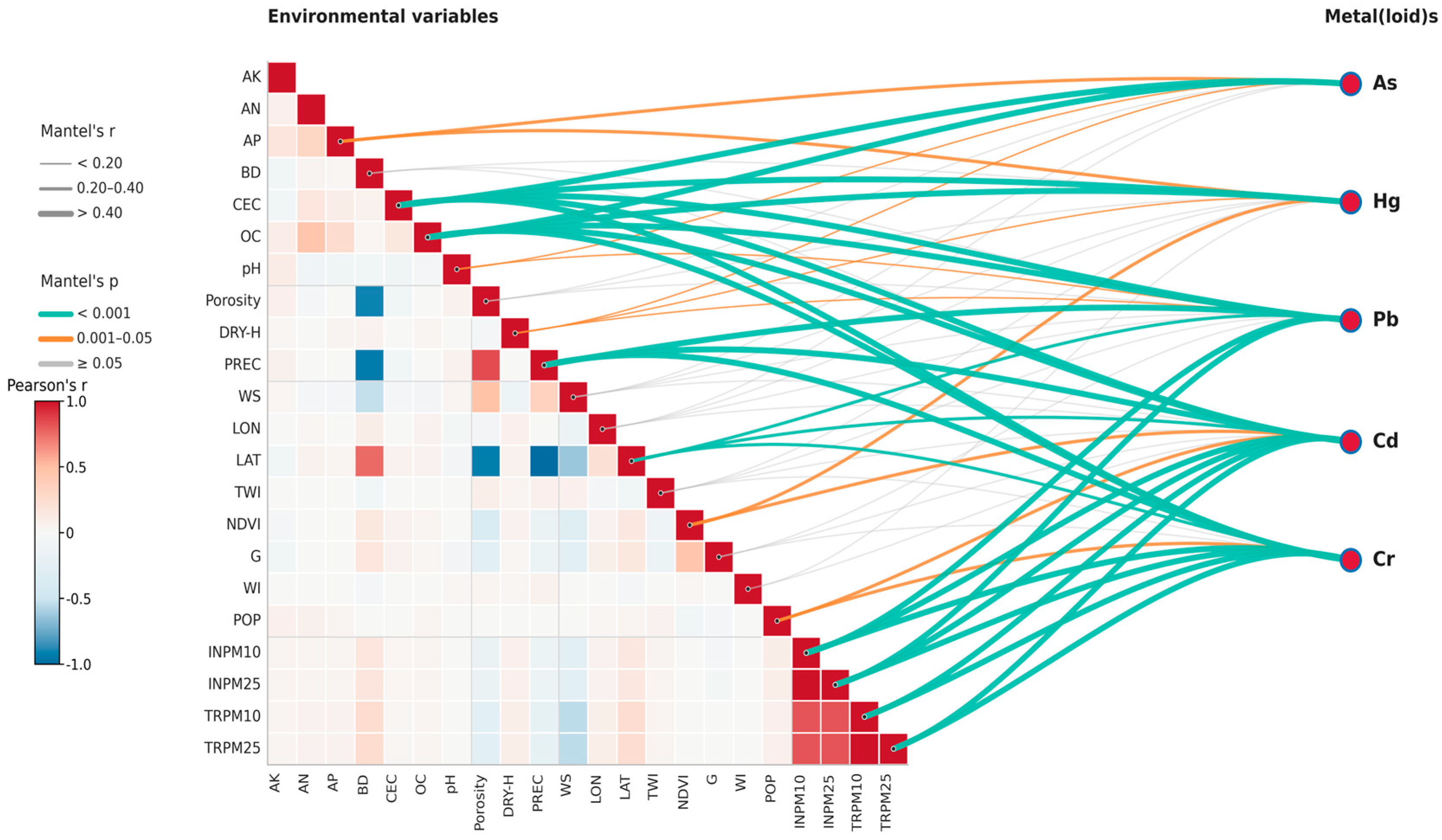
The Pearson correlation matrix revealed a clear covariance structure among the environmental variables (Figure 4), with particulate matter indicators (INPM10, INPM25, TRPM10, and TRPM25) showing strong positive intercorrelations, indicative of a common anthropogenic signal. Vegetation-related indices also exhibited coherent positive relationships, whereas several meteorological and geographic variables formed spatially structured gradients. Mantel analysis further demonstrated that soil physicochemical properties were most strongly associated with heavy metal distributions, as evidenced by multiple thick and highly significant links between the soil-property cluster and As, Hg, Pb, Cd, and Cr. These results indicate that the spatial heterogeneity of soil heavy metals is more strongly constrained by intrinsic soil conditions than by meteorological or geographic factors alone.

Table 2. Model performance with five major heavy metal(loid)s as targets.

Model/Heavy Metal(loid)s	As	Hg	Cd	Cr	Pb
RF	R2 = 0.258 RMSE = 1.839	R2 = 0.270 RMSE = 0.015	R2 = 0.079 RMSE = 0.076	R2 = 0.367 RMSE = 12.406	R2 = 0.068 RMSE = 4.542
XGBoost	R2 = 0.217 RMSE = 1.889	R2 = 0.239 RMSE = 0.016	R2 = 0.043 RMSE = 0.077	R2 = 0.339 RMSE = 12.677	R2 = 0.033 RMSE = 4.625
ET	R2 = 0.284 RMSE = 1.807	R2 = 0.348 RMSE = 0.015	R2 = 0.089 RMSE = 0.076	R2 = 0.424 RMSE = 11.826	R2 = 0.058 RMSE = 4.565
LightGBM	R2 = 0.236 RMSE = 1.867	R2 = 0.280 RMSE = 0.015	R2 = −0.045 RMSE = 0.081	R2 = 0.304 RMSE = 13.000	R2 = −0.012 RMSE = 4.732
LASSO-stacking	R2 = 0.291 RMSE = 1.803	R2 = −0.015 RMSE = 0.018	R2 = −0.002 RMSE = 0.079	R2 = 0.432 RMSE = 11.848	R2 = 0.041 RMSE = 4.607

summarizes the predictive performance of the LASSO-stacking ensemble and individual base models. In the LASSO-stacking model, the RMSE values for As, Hg, Cd, Cr, and Pb were 1.803, 0.018, 0.079, 11.848, and 4.607, respectively. Overall, As and Cr were predicted more effectively by the selected features, either within the LASSO-stacking framework or by individual base models. In contrast, Cd and Pb showed relatively low R² values, indicating that the variables included in this study captured only part of the factors controlling their concentrations in soil. The LASSO-stacking model did not consistently outperform the individual tree-based learners. This result may be attributed to the relatively high correlation and limited complementarity among the predictions of the base models, as well as the linear and regularized structure of the LASSO meta-learner. In comparison, the tree-based models were better able to capture nonlinear relationships and interactions between the environmental predictors and heavy metal(loid) concentrations. Nevertheless, the overall out-of-sample predictive performance remained modest, indicating that additional site-specific source and management variables may be required to improve prediction accuracy.

Among the five target heavy metals, the LASSO-stacking model achieved improved predictive performance for As, Cr, and Pb relative to the best-performing single base learners. This suggests that the proposed architecture can effectively enhance prediction accuracy by exploiting complementary strengths across multiple models, highlighting the value of ensemble-learning strategies for complex analytical tasks. Notably, Pb exhibited the largest gain (although the improvement primarily shifted R² from negative in the strongest single model to positive), implying that the Pb–feature relationship is particularly complex.

By contrast, the LASSO-stacking model performed substantially worse than individual base models for Cd and Hg. One plausible explanation is that these two metals display comparatively homogeneous spatial patterns or weaker heterogeneity in their feature dependencies, such that a single model is sufficient to capture the dominant variability. Cd and Hg may also be more strongly associated with a limited set of key predictors, enabling relatively simple learners (e.g., Extra Trees Regressor or Random Forest) to recover the main signal. Aggregating outputs from multiple base models, the stacking procedure may also introduce additional noise or interference from less-informative learners, thereby degrading overall performance.

Accordingly, for As, Cr, and Pb, we will conduct SHAP analyses based on the LASSO-stacking model to examine the contributions of specific features to target prediction. SHAP can quantify each feature’s contribution to the model output, providing a ranked feature-importance profile and enabling deeper interpretation of the model’s decision process. For Cd and Hg, SHAP-based interpretation will be performed using the ET model, aiming to capitalize on ET’s relative advantage in predicting Hg and Cd to identify the dominant features and their contributions to prediction.

3.2. SHAP-Based Interpretation of Model-Derived Associations for Heavy Metal(loid)s Contamination in Ningxia Farmland Soils

In addition to evaluating predictive performance, model interpretation was conducted to examine how the fitted machine learning models used different predictors when estimating soil heavy metal(loid) concentrations. SHAP values were used to quantify the contribution of each predictor to model outputs and to visualize the direction and magnitude of feature effects. It should be noted that SHAP values explain the behavior of a fitted model and do not establish causal relationships. Therefore, the SHAP results in this study are interpreted as model-derived statistical associations rather than direct evidence of causality.

Given the element-specific differences in model performance, SHAP interpretation was conducted using the best-performing or relatively most suitable model for each target element rather than applying a single model uniformly to all metals. Specifically, SHAP analyses were based on the LASSO-stacking model for As and Cr, the ET model for Hg and Cd, and the RF model for Pb. For elements with relatively better predictive performance, such as As and Cr, SHAP results were used to identify model-derived environmental associations. For elements with weak predictive performance, particularly Cd and Pb, SHAP outputs were interpreted only as exploratory indications of possible covariate associations and should not be regarded as robust evidence of dominant environmental drivers. Mechanistic explanations are discussed only as process-consistent interpretations supported by previous studies and require further validation through experimental, temporal, or process-based evidence.

3.2.1. As Interpretation

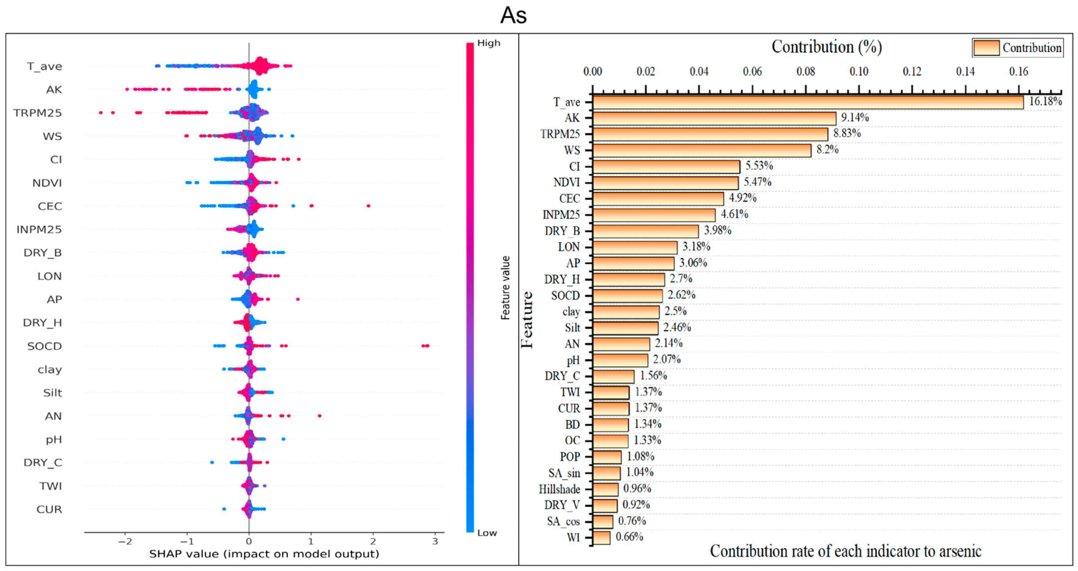
The SHAP beeswarm plot based on the LASSO-stacking model indicates that AK, SS, PET, clay, PREC, CEC, sand, pH, AP, and OC were the highest-ranked predictors associated with model-predicted As concentrations, with additional but smaller contributions from anthropogenic proxies, such as CI, TRPM10, and INPM10, and spatial–topographic descriptors, such as LAT and CUR (Figure 5). Overall, the model captured a compound signal integrating regional hydroclimatic context, soil carrier properties, and spatially structured management intensity. The broad dispersion of SHAP values across samples indicates pronounced context dependence and potential interactions among covariates.

AK ranked as the most influential proxy of soil background. It showed a consistent directional pattern: high AK values were predominantly associated with negative SHAP values, whereas low AK values more often produced positive SHAP values, implying higher predicted soil As under low-AK conditions. Because arsenic behavior in soils is strongly governed by anion-related processes, including arsenate and arsenite reactions, AK is more plausibly interpreted as an integrated proxy for soil type, parent material, and fertility background [93], which co-varies with regional As hotspots.

Climatic variables exhibited a coherent pattern: high SS and PET values contributed positively, whereas high PREC values contributed negatively. This association is consistent with possible processes such as reduced leaching, enhanced near-surface retention, and hydroclimate-related changes in soil moisture conditions. Drier environments may also coincide with stronger atmospheric deposition or surface accumulation backgrounds, but these interpretations should be considered process-consistent hypotheses rather than causal conclusions from SHAP alone [94].

Among soil properties, high CEC generally contributed positively, consistent with the interpretation that soils with greater exchange capacity and more reactive surfaces can promote As retention on the solid phase [95]. Texture-related predictors showed a more complex but interpretable pattern: higher sand and gravel contents generally produced negative SHAP values, consistent with fewer reactive surfaces and dilution by coarse fractions. Higher clay content tended to produce negative contributions in this region, suggesting that clay-rich settings were not necessarily As-enriched. This pattern likely reflects parent-material effects, spatial co-variation, or multivariate coupling rather than a simple adsorption control [96]. High AP produced predominantly positive contributions, indicating higher predicted As under elevated available phosphorus. Two interpretations are plausible: phosphate may compete with arsenate for sorption sites on Fe/Al oxides [97], promoting As desorption and redistribution, and AP may act as an indicator of soil fertility and fertilization intensity. The positive contribution of CI further supports an association between agricultural intensity and As spatial patterns. Higher pH showed an overall negative tendency. Because As sorption commonly weakens as pH increases, this negative relationship with solid-phase As may reflect reduced retention of anionic As(V) under surface deprotonation, increased electrostatic repulsion, and competition with OH⁻, carbonate, and phosphate for reactive sites. This pH-driven shift toward the aqueous phase could enhance mobility and, under percolating water flow, promote leaching losses that lower residual As in soil [98,99]. Particulate emission proxies, including TRPM10, INPM10, and TRPM25, ranked lower and clustered closer to zero, suggesting limited incremental explanatory power after accounting for climate and soil attributes. Their mixed signs indicate context dependence, potentially modulated by location, terrain-driven redistribution, and soil carrier properties. Overall, natural hydroclimatic and soil factors appear to dominate regional As heterogeneity, whereas anthropogenic proxies may exert secondary modulation in specific settings.

3.2.2. Hg Interpretation

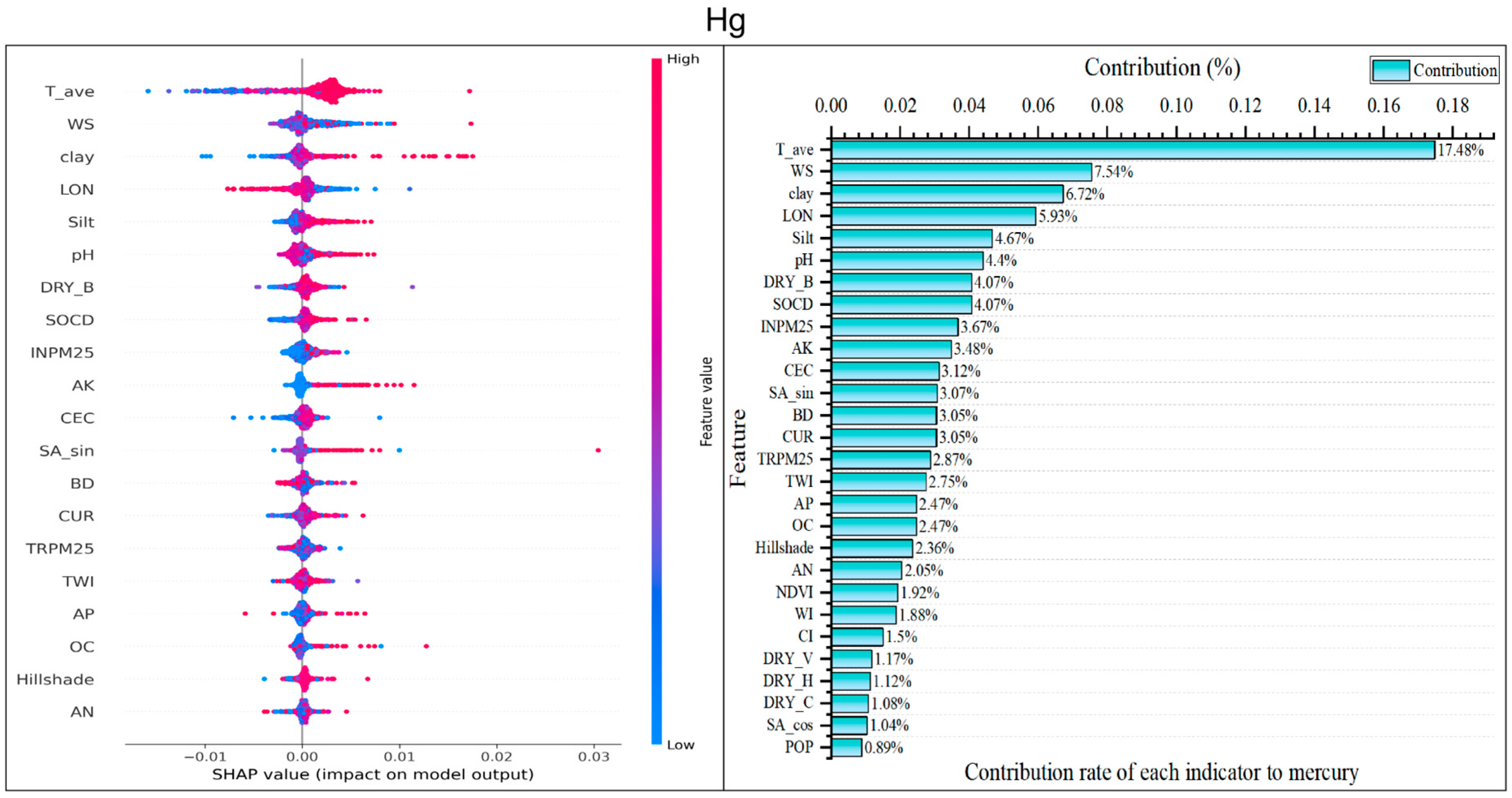
The SHAP beeswarm plot derived from the ET model was used to interpret model-derived associations for Hg because ET showed the best predictive performance among the tested models for this element. The leading predictors included PREC, temperature-related variables, SS, RHU, TWI, WS, and spatial–topographic covariates such as LAT, DEM, and LON (Figure 6). These variables should be interpreted as predictors associated with model-predicted Hg concentrations, not as direct causal controls.

Several leading predictors showed clear directional patterns. High PREC values were concentrated on the negative SHAP side, indicating that wetter conditions tended to reduce predicted Hg accumulation [100], whereas low PREC values contributed positively. Temperature metrics generally showed the opposite tendency, with higher T_min, T_max, and T_ave values corresponding to positive SHAP values. Warmer conditions may enhance vegetation productivity and canopy-mediated uptake of atmospheric Hg, increasing Hg transfer to soils via litterfall and throughfall and promoting accumulation in the soil organic pool [101]. Higher RHU predominantly showed negative contributions, whereas lower RHU showed positive contributions, suggesting that humid conditions may suppress Hg accumulation. For WS, lower values more often contributed positively, whereas higher values were neutral or weakly negative, consistent with enhanced Hg accumulation under lower atmospheric dispersion potential [102].

Among land-surface and soil-related variables, higher TWI values tended to contribute positively, although with substantial scatter, indicating that wetter topographic settings may enhance Hg accumulation in soil (Figure 6). SOCD also exhibited predominantly positive SHAP values at higher levels, consistent with stronger predicted Hg accumulation in soils with greater organic carbon stocks. This pattern may reflect strong complexation of Hg(II) with organic ligands, especially reduced sulfur groups, which enhances Hg retention and promotes legacy Hg accumulation in organic-rich soils. DOC-mediated complexation and colloid transport may also regulate solid-solution partitioning and redistribution [103]. DEM and other terrain descriptors, including slope and CUR, showed smaller average effects but occasional large positive contributions, pointing to context-dependent topographic controls. LAT and LON showed mixed SHAP signs and relatively wide dispersion, indicating spatially structured heterogeneity that may reflect regional gradients or interactions not fully captured by individual covariates. Particulate-matter proxies, including TRPM25 and TRPM10, ranked lowest and clustered tightly around zero, suggesting limited incremental explanatory power for Hg after climate, soil, and topographic factors were accounted for.

3.2.3. Cd Interpretation

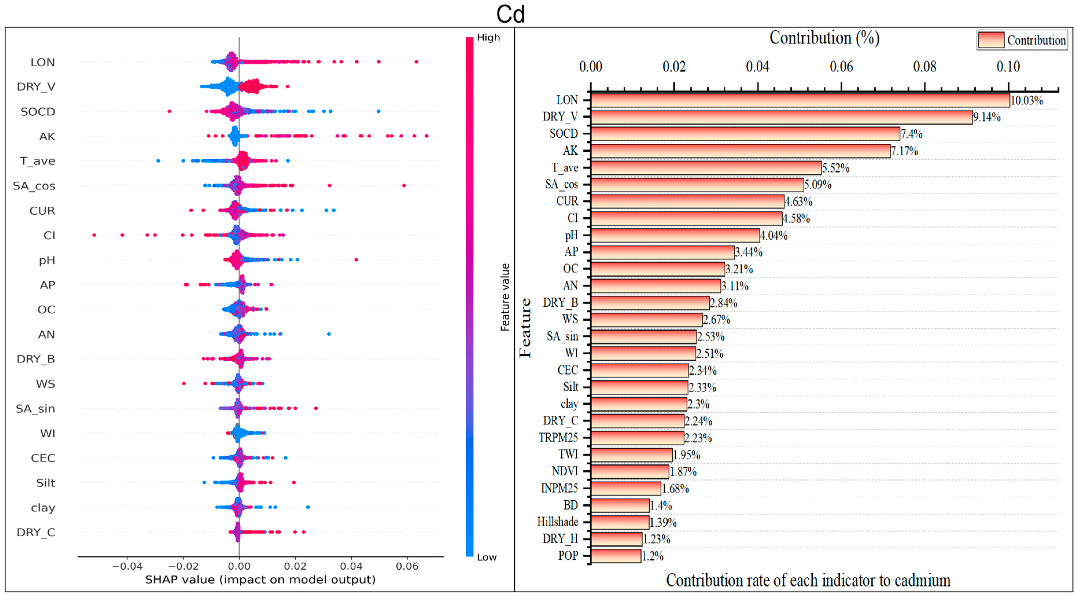
The SHAP beeswarm plot derived from the ET model was used to examine model-derived associations for Cd. However, because the predictive performance for Cd was weak, these SHAP results should be regarded as exploratory and should not be interpreted as robust evidence of dominant environmental drivers. The highest-ranked predictors included LON, CEC, aspect components, and terrain curvature (Figure 7), suggesting that the fitted model captured spatial gradients and soil-retention-related associations, but the low predictive skill indicates that important Cd-related processes may not be fully represented by the current feature set.

LON showed a pronounced directional pattern: high values were predominantly associated with positive SHAP values, whereas low values clustered on the negative side, suggesting a marked longitudinal gradient or spatially structured heterogeneity in Cd concentrations. CEC showed a consistent positive association, with higher values mainly producing positive SHAP values. This positive relationship suggests that Cd accumulation is closely linked to the abundance of reactive, negatively charged sorption sites. Higher CEC typically reflects greater contributions from clay minerals and soil organic matter, both of which provide extensive exchange surfaces and increase the capacity of soil to retain Cd, predominantly as Cd²⁺ [104]. Co-variation in CEC with fine-particle content and organic matter may further enhance Cd enrichment through adsorption to clay-organic complexes and association with Fe/Mn (hydr)oxides carried by fine fractions [105].

Several predictors showed negative contributions at higher values. Specifically, CUR, SOCD, gravel, AP, and T_min tended to show negative SHAP values when feature values were high, whereas lower values more frequently contributed positively (Figure 7). These patterns suggest that the upper ranges of these variables may suppress predicted Cd concentrations. Climate-related variables showed coherent responses: high T_ave, T_max, and PET values generally contributed positively, suggesting that warmer and more evaporative conditions were associated with increased Cd concentrations. Elevated temperature can also alter Cd-DOM binding through changes in dissolved organic matter composition and aromaticity in contaminated agricultural soils [106]. Dryness-related indices, including DRY_R, DRY_V, and DRY_G, predominantly showed positive SHAP values at higher levels, indicating a tendency for Cd predictions to increase under drier environmental settings.

Among soil and management variables, CI tended to contribute positively at higher values. Increased cropping intensity may involve more frequent tillage and soil disturbance, which can facilitate the release of previously retained Cd into the soil solution [107]. Fertilization and irrigation can further accelerate Cd transformation from solid-bound forms to more soluble fractions that are more readily available for plant uptake [108]. High-intensity cropping also increases root density and rhizosphere activity, which may enhance Cd desorption during water and nutrient uptake [109]. In addition, acidic conditions increase Cd solubility and favor its release from soil solids into the soil solution [110]. The long-term use of fertilizers and pesticides containing trace Cd may also contribute to gradual Cd accumulation in agricultural soils [111].

3.2.4. Cr Interpretation

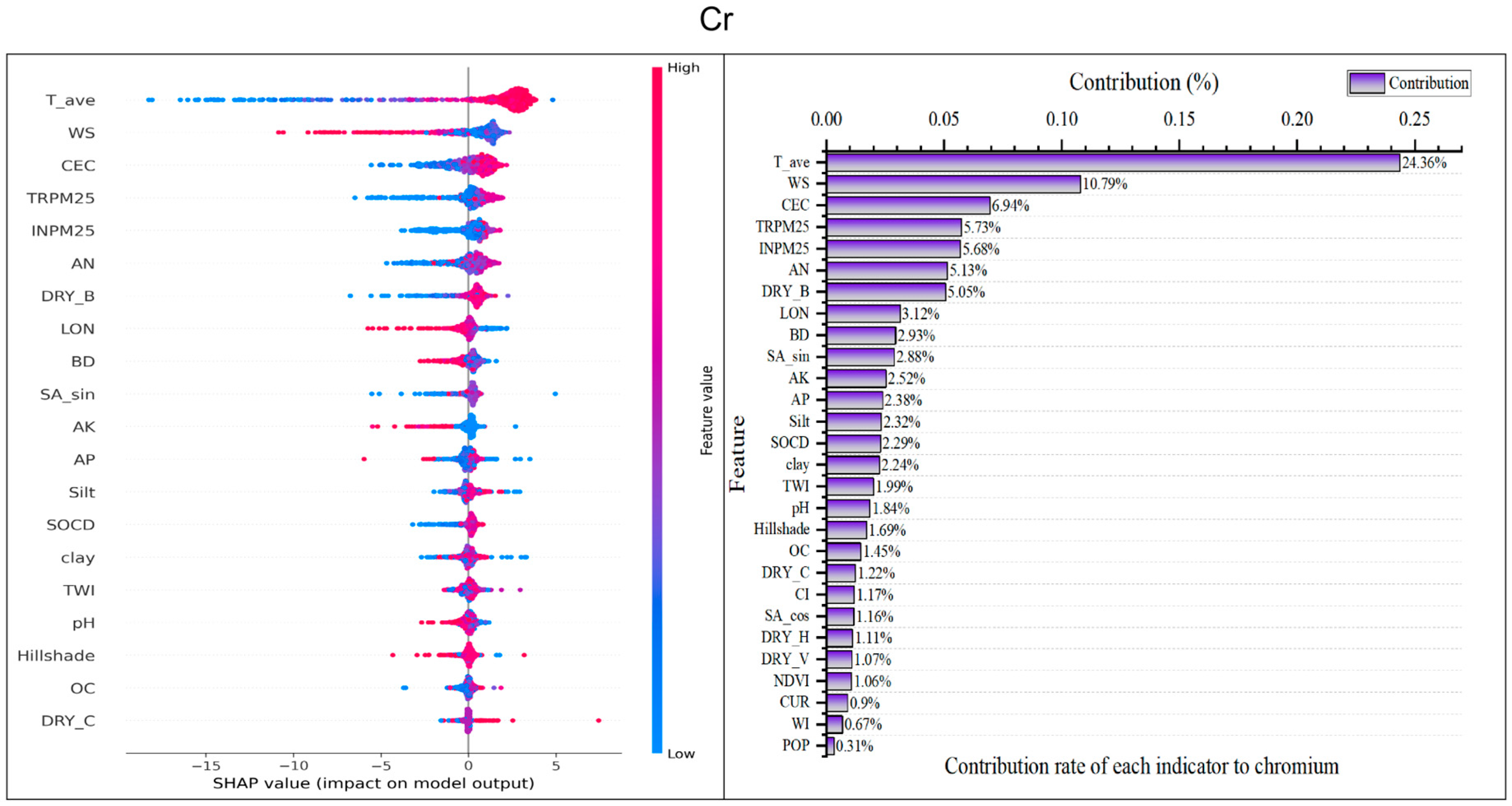
The SHAP beeswarm plot for the LASSO-stacking model showed that PREC, PET, DEM, porosity, temperature-related variables, INPM25, and soil bulk density were among the highest-ranked predictors associated with model-predicted Cr concentrations (Figure 8). Compared with Cd and Pb, the Cr model showed relatively better predictive performance; therefore, the SHAP results provide more reliable model-derived associations, although they still should not be interpreted as causal evidence.

A coherent directional pattern was observed: high precipitation (PREC) was predominantly associated with negative SHAP values, whereas low PREC values clustered on the positive side. This pattern implies that increased soil Cr concentrations under drier conditions may reflect reduced hydrologic flushing and enhanced near-surface accumulation. Under limited precipitation and weaker percolation, downward leaching and lateral export of Cr-bearing fine particles are constrained, allowing Cr to be retained and progressively stored in the solid phase [112]. Conversely, high PET values contributed positively, indicating that stronger evaporative demand was associated with increased Cr. Temperature metrics also exhibited mainly positive contributions at higher values. These patterns may be consistent with stronger dust loading and dry deposition in arid settings, but this explanation remains a process-consistent interpretation rather than a causal conclusion.

DEM showed a clear high-value-negative-SHAP and low-value-positive-SHAP pattern, suggesting higher predicted Cr concentrations in lower-elevation settings. This association is consistent with the preferential deposition of fine particles and associated elements in lowlands and convergent landscape positions. Contributions from SA_sin and hillshade further indicate that aspect-related microenvironments and terrain shading may shape Cr heterogeneity [113].

Higher INPM25, TRPM25, and TRPM10 values were generally associated with positive SHAP values, indicating that stronger industrial and traffic emission intensity tended to elevate predicted Cr concentrations. Because Cr is commonly present in industrial aerosols and traffic-related particulate matter, this pattern supports a potential role of atmospheric deposition in locally modulating surface-soil Cr [114]. Nevertheless, their overall importance was lower than that of hydroclimatic and topographic predictors, suggesting that natural background controls dominate Cr variability at the study-region scale, with anthropogenic signals acting as secondary modifiers.

3.2.5. Pb Interpretation

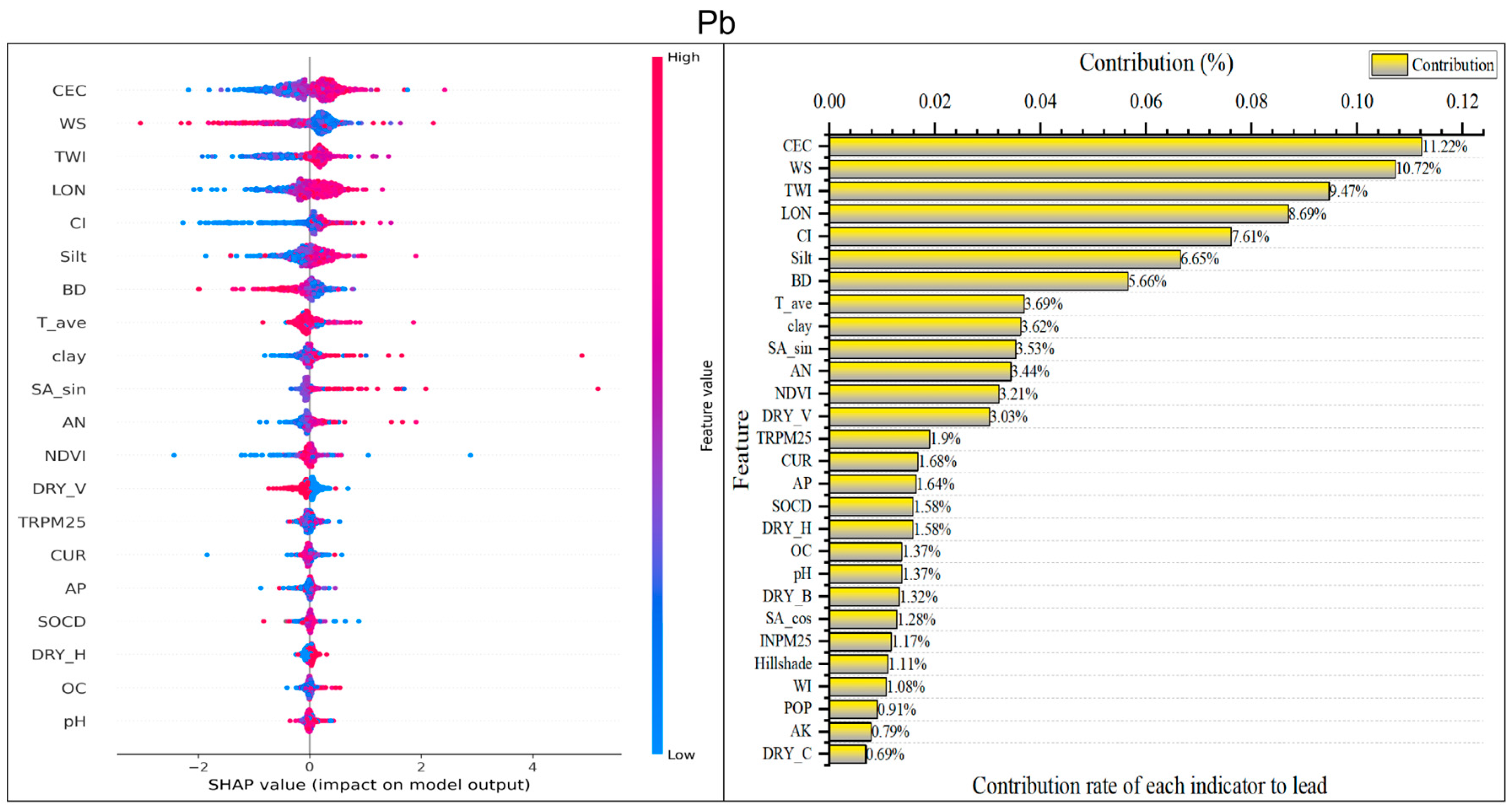
The SHAP beeswarm plot for the LASSO-stacking model indicates that predicted soil Pb was primarily governed by spatial structure (LAT and LON) and terrain–hydrological setting (TWI and related topographic descriptors), with secondary modulation by atmospheric dispersion conditions (WS), soil physical properties (Clay, Porosity, OC), and agricultural intensity (CI). According to mean absolute SHAP values, LAT and TWI were the most influential predictors, followed by WS, clay, SS, porosity, LON, SA_sin, and CI (Figure 9).

Soil geochemical background and pedogenic properties appear to provide the fundamental framework for Pb accumulation. Among all predictors, CEC showed the highest contribution, followed by silt, clay, bulk density, pH, and carbon-related variables (OC and SOCD). The SHAP beeswarm plot further showed that higher CEC and finer-textured fractions generally corresponded to positive SHAP values, indicating enhanced Pb accumulation under greater sorption capacity and a larger specific surface area. This pattern is consistent with the well-known geochemical behavior of Pb as a strongly particle-reactive element with high affinity for exchange sites, clay minerals, and soil colloids. However, because of their weak predictive performance, these relationships should be interpreted as possible associations rather than definitive evidence of Pb retention mechanisms.

Topography-driven redistribution is a key mechanism shaping landscape-scale Pb enrichment. The high importance of TWI, CI, curvature, and solar-radiation-related terrain variables indicates that Pb hotspots are strongly associated with runoff convergence, sediment transport, and depositional environments. The positive SHAP response of high TWI values suggests that wetter convergence zones and lower slope positions function as sinks for Pb accumulation. This finding implies that Pb is not only preserved near initial input locations but also undergoes secondary migration and re-enrichment through erosion, lateral transport, and microtopographic deposition. Thus, the observed Pb pattern is best interpreted as the coupled result of regional inputs and terrain-mediated concentration effects.

The prominence of wind speed (WS), together with the non-negligible contributions of PM2.5-related variables, suggests that atmospheric deposition is an important anthropogenic pathway for soil Pb. Given the established association of Pb with aerosols, combustion-derived particles, and road dust, this pattern points to diffuse external inputs derived primarily from traffic emissions, industrial activities, and fossil-fuel combustion, followed by regional transport and deposition onto the soil surface. The relatively modest contribution of population density implies that Pb contamination is not controlled solely by present-day urban intensity or local settlement patterns but more likely reflects long-term, spatially diffuse atmospheric loading at the regional scale.

Taken together, the SHAP outputs support the interpretation that soil Pb in the study area reflects a mixed source regime dominated by geogenic background and anthropogenic atmospheric deposition, with topographic–hydrological processes exerting a strong secondary control on redistribution and local enrichment. Although regional covariates such as emission inventories, climate variables, cropping intensity, and wastewater irrigation can capture broad source-pressure gradients, they cannot fully resolve plot-scale or sub-meter heterogeneity in soil heavy metal(loid) concentrations. Therefore, the model-derived associations reported here should be interpreted as regional-scale patterns rather than direct site-level causal mechanisms. In addition, some predictors may act as surrogates for unmeasured historical or local factors. This limitation is particularly relevant for Pb, whose accumulation may reflect the combined effects of geogenic background, atmospheric deposition, long-term agricultural inputs, sludge or organic amendment use, and other legacy sources. Because detailed historical records were not available, the present framework cannot fully distinguish contemporary drivers from legacy pollution. Future work should integrate historical emission inventories, field management records, fertilizer and sludge application histories, isotopic tracers, and finer-scale sampling to improve source attribution and local risk assessment.

3.3. Integrated Source Apportionment and Environmental Interpretation of Heavy Metals

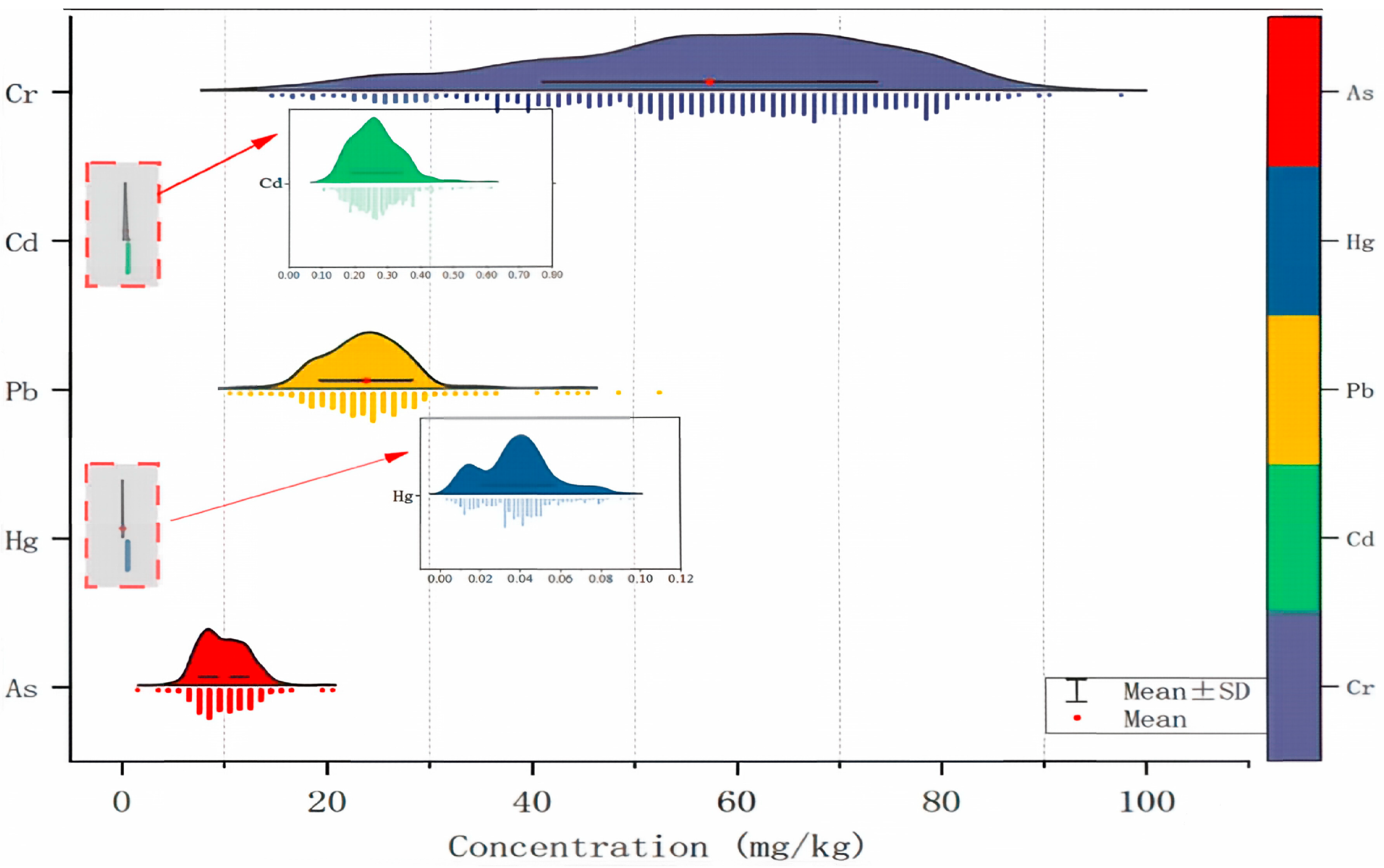
Based on the measured metal concentrations, the cultivated soils of Ningxia generally had a moderate pollution level, although a certain degree of heavy metal contamination was observed, with Cd and Hg identified as the major pollutants (Figure 10). To further elucidate the potential sources of these metals, a combined framework integrating PCA, PMF, and machine learning interpretation was adopted.

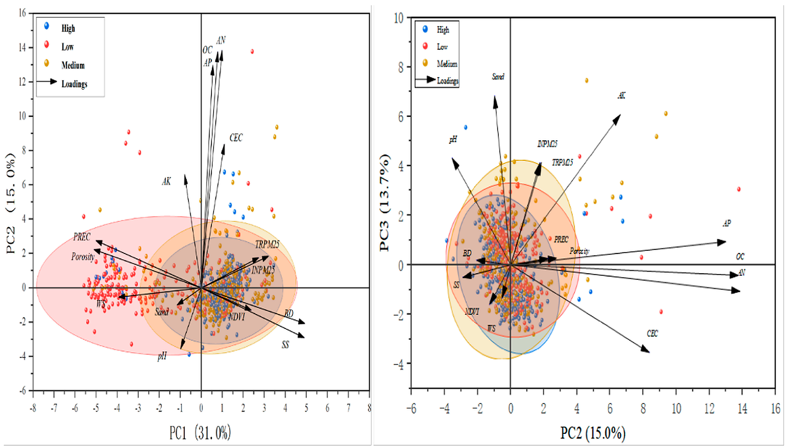
PCA was first applied to extract the dominant compositional structure of the five heavy metals. Three principal components were retained, with a cumulative explained variance of 59.7%, indicating that they captured most of the source-related information in the dataset (Figure 11). PC1 explained 31% of the total variance and was characterized by a strong Cd contribution. PC2 accounted for 15% of the variance and was mainly associated with Hg, whereas PC3 explained 13.7% and was characterized by relatively high loadings of Pb, As, and Cr. These results suggest that the five metals were not controlled by a single common source but instead reflected multiple source types and environmental processes.

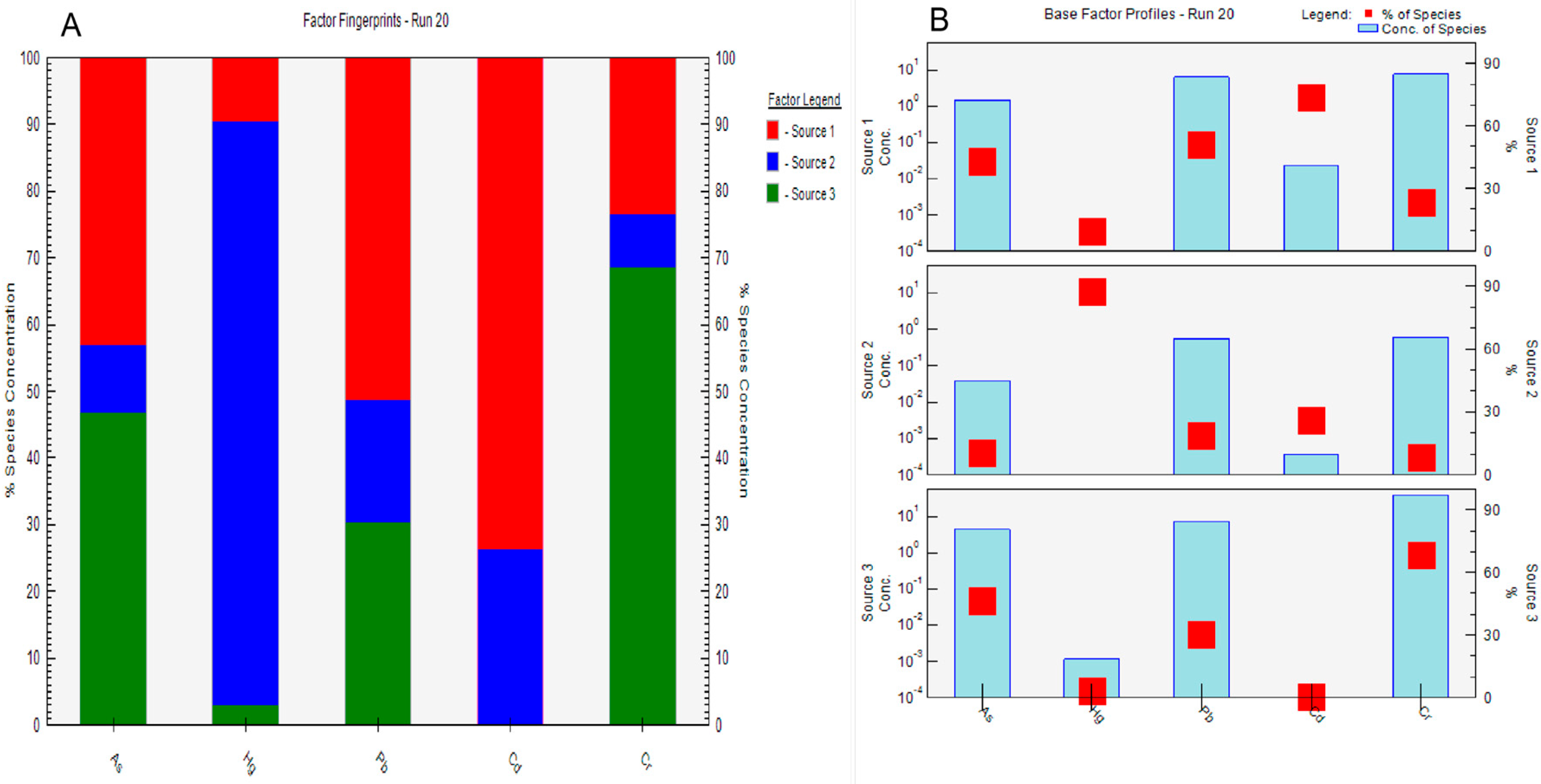
To further quantify the contributions of different source categories, the PMF model was applied. A three-factor solution was selected because it yielded the minimum Q value and satisfactory model performance (Figure 12). The coefficients of determination (R²) between observed and predicted concentrations ranged from 0.68 to 0.92, indicating acceptable simulation accuracy and supporting the robustness of the selected PMF solution. The three factors showed clear compositional contrasts. Source 1 contributed predominantly to Cd (73.8%), Source 2 was dominated by Hg (87.6%), and Source 3 contributed most strongly to Cr (68.4%) and substantially to As (46.7%). These factor profiles indicate marked source differentiation among the five metals.

PMF primarily resolves latent source structure through source profiles and percentage contributions, but it provides limited information on the environmental contexts under which elevated concentrations occur. This limitation is particularly relevant for As, Cr, and Pb, whose distributions may be influenced not only by source inputs but also by background gradients, transport pathways, and post-depositional redistribution. We therefore interpreted the PMF results together with SHAP outputs derived from the LASSO-stacking and ET models.

In this study, SHAP analysis was used to interpret the fitted machine learning models and to identify model-derived associations between predictor variables and predicted metal concentrations. The SHAP results should be interpreted as complementary statistical information rather than causal evidence or independent source apportionment. For Hg, the leading predictors were mainly hydroclimatic and terrain variables, with important contributions from precipitation, temperature metrics, topographic wetness, and wind-related factors. This pattern suggests that, although Hg was strongly concentrated in one PMF factor, its accumulation was further conditioned by atmospheric input efficiency and landscape convergence. Pb was more strongly associated with spatial descriptors and soil carrier properties, including geographic coordinates, topographic wetness, wind speed, and fine-particle retention characteristics, indicating that its enrichment reflected both anthropogenic influence and environmental redistribution. Cr was controlled primarily by background environmental variables, including climatic factors, terrain-related descriptors, and soil physical properties, while air-pollution proxies exerted only secondary effects, supporting a stronger geogenic or background signature. Cd showed stronger dependence on spatial descriptors, CEC, soil organic carbon density, curvature, and aspect-related variables, indicating the importance of exchange sites, carbon carriers, and terrain-driven redistribution. As was influenced by soil nutrient status, hydroclimatic conditions, and retention-related soil properties, reflecting mixed control by environmental background and surface-process regulation.

When interpreted together, the PMF and SHAP results provide a more complete understanding of heavy metal sources in Ningxia farmland soils. PCA and PMF address where the metals likely originate by identifying source patterns and contribution structures, whereas SHAP-based machine learning analysis explains where and under what environmental conditions elevated concentrations are more likely to occur. In this sense, machine learning does not replace PMF in source apportionment; rather, it complements PMF by providing process-oriented evidence for the environmental expression of source-associated metals at the sample scale. This integrated framework is particularly useful for farmland heavy metal assessment because it links source identification with spatially explicit environmental controls, thereby providing a stronger basis for high-resolution risk mapping and targeted soil management.

3.4. Policy Implications

Based on the PMF source-apportionment results and the model-derived SHAP associations, cropland contamination in Ningxia appears to reflect the combined effects of controllable anthropogenic inputs, natural background conditions, and environmental redistribution. Anthropogenic proxies, including industrial and traffic particulate emissions, population density, cropping intensity, and wastewater irrigation, were associated with the predicted concentrations of some metals, suggesting that these variables may help identify priority areas for source-oriented management. Soil properties (CEC, SOC, texture, pH, and porosity) and terrain-climate factors (TWI, DEM, PREC, PET, and WS) also modulate retention, redistribution, and spatial susceptibility. Cropland pollution control should therefore adopt a tiered strategy that prioritizes anthropogenic source reduction while using non-anthropogenic factors to delineate high-susceptibility zones for fine-scale risk management.

(1)

Industrial and Energy Emission Abatement Coupled With Cropland Protection: The PMF results indicate that Hg was mainly associated with an industrial atmospheric deposition source, while model-derived associations suggest that emission- and dispersion-related variables may also be relevant to the spatial expression of Pb and Cr in some areas. Therefore, industrial emission control and deposition monitoring should focus primarily on Hg, while also considering Pb and Cr in downwind or emission-affected croplands.

(2)

Traffic-Source and Road-Dust Control With Buffer-Based Land Management: Where traffic-related particulate proxies show incremental explanatory value, near-road croplands should be treated as priority areas for monitoring and preventive management, particularly for Pb and Cr. Measures may include graded buffer zones, ecological barriers, road-dust suppression, and joint monitoring of road dust and topsoil.

(3)

Control of Agricultural Inputs and Management Intensity Through Traceability and Auditability: The PMF results indicate that Cd was mainly associated with agricultural inputs. Therefore, management should prioritize reducing Cd inputs from fertilizers, organic amendments, irrigation water, and other agricultural materials. For As and Pb, agricultural management should be considered as a potential contributing pathway only where supported by local evidence, because their accumulation may also reflect natural background, atmospheric deposition, and historical legacy inputs.

4. Conclusions

This study developed a source-integrated and interpretable modeling framework to identify the dominant sources and environmental drivers of heavy metal(loid) contamination in farmland soils of Ningxia. By combining receptor-model source apportionment with machine learning interpretation, the framework links source contribution patterns with the soil, climatic, topographic, and anthropogenic conditions under which metal enrichment occurs.

The results indicate that farmland soils in Ningxia are affected by multiple source processes rather than a single dominant input pathway. Cadmium was mainly associated with agricultural inputs, mercury was closely related to industrial atmospheric deposition, and chromium and arsenic were largely influenced by natural background conditions, including parent material and regional geological inheritance. These source patterns suggest that metal accumulation in farmland soils reflects the combined effects of external inputs, geochemical background, and environmental redistribution.

Interpretable machine learning results further showed that source-associated enrichment was regulated by distinct environmental controls. Soil retention capacity, spatial gradients, hydroclimatic conditions, topographic wetness, and agricultural intensity jointly shaped the spatial expression of heavy metal(loid) contamination. These findings demonstrate that machine learning interpretation can complement source apportionment by explaining why source-related metal accumulation is more likely to occur in specific environmental settings.

Overall, the proposed framework provides a more informative basis for farmland soil contamination assessment than source apportionment or predictive modeling alone. It supports a shift from concentration-based assessment toward source- and process-oriented management by identifying not only where contamination occurs, but also which source pathways and environmental conditions require priority attention. In practical terms, this approach can help delineate priority monitoring zones, distinguish controllable anthropogenic inputs from natural background contributions, and support more targeted prevention and control strategies. For Ningxia, management efforts should prioritize reducing cadmium inputs from agricultural activities, controlling mercury deposition from industrial emissions, and incorporating geological background into the assessment of chromium and arsenic risks. Future studies should further integrate source-specific activity data, long-term monitoring, and crop uptake information to improve the robustness of source attribution and risk-based soil management.

References

1. Hou, D.; Jia, X.; Wang, L.; McGrath, S.P.; Zhu, Y.G.; Hu, Q.; Zhao, F.-J.; Bank, M.S.; O’cOnnor, D.; Nriagu, J. Global soil pollution by toxic metals threatens agriculture and human health. Science 2025, 388, 316–321. [Google Scholar] [CrossRef] [PubMed]
2. Khan, S.; Naushad, M.; Lima, E.C.; Zhang, S.; Shaheen, S.M.; Rinklebe, J. Global soil pollution by toxic elements: Current status and future perspectives on the risk assessment and remediation strategies–A review. J. Hazard. Mater. 2021, 417, 126039. [Google Scholar] [CrossRef] [PubMed]
3. Hou, D.; O’Connor, D.; Igalavithana, A.D.; Alessi, D.S.; Luo, J.; Tsang, D.C.W.; Sparks, D.L.; Yamauchi, Y.; Rinklebe, J.; Ok, Y.S. Metal contamination and bioremediation of agricultural soils for food safety and sustainability. Nat. Rev. Earth Environ. 2020, 1, 366–381. [Google Scholar] [CrossRef]
4. Mai, X.; Tang, J.; Tang, J.; Zhu, X.; Yang, Z.; Liu, X.; Zhuang, X.; Feng, G.; Tang, L. Research progress on the environmental risk assessment and remediation technologies of heavy metal pollution in agricultural soil. J. Environ. Sci. 2025, 149, 1–20. [Google Scholar] [CrossRef]
5. Rashid, A.; Schutte, B.J.; Ulery, A.; Deyholos, M.K.; Sanogo, S.; Lehnhoff, E.A.; Beck, L. Heavy metal contamination in agricultural soil: Environmental pollutants affecting crop health. Agronomy 2023, 13, 1521. [Google Scholar] [CrossRef]
6. Cai, Z.; Ren, B.; Xie, Q.; Deng, X.; Yin, W.; Chen, L. Assessment of health risks posed by toxicological elements of the food chain in a typical high geologic background. Ecol. Indic. 2024, 161, 111981. [Google Scholar] [CrossRef]
7. Kumar, P.; Kumar, S.; Singh, R.P. Severe contamination of carcinogenic heavy metals and metalloid in agroecosystems and their associated health risk assessment. Environ. Pollut. 2022, 301, 118953. [Google Scholar] [CrossRef] [PubMed]
8. Chai, L.; Wang, Y.; Wang, X.; Ma, L.; Cheng, Z.; Su, L. Pollution characteristics, spatial distributions, and source apportionment of heavy metals in cultivated soil in Lanzhou, China. Ecol. Indic. 2021, 125, 107507. [Google Scholar] [CrossRef]
9. Guan, Y.; Zhang, N.; Li, B.; Ma, T.; Wu, W.; Shi, R. A novel evaluation of farmland soil environmental risk integrating heavy metal (loid) pollution risk and industrial risk potential. Stoch. Environ. Res. Risk Assess. 2025, 39, 3085–3102. [Google Scholar] [CrossRef]
10. Wu, J.; Huang, C. Machine learning-supported determination for site-specific natural background values of soil heavy metals. J. Hazard. Mater. 2025, 487, 137276. [Google Scholar] [CrossRef] [PubMed]
11. Alharbi, T.; Nour, H.E.; El-Sorogy, A.S.; Al-Kahtany, K.; Giacobbe, S.; Alarifi, S.S. Evaluation of health risks and heavy metals toxicity in agricultural soils in Central Saudi Arabia. Environ. Monit. Assess. 2025, 197, 419. [Google Scholar] [CrossRef] [PubMed]
12. Nour, H.; Ramadan, F.; Abdel Wahed, N.; Rakha, A. Spatial distribution and contamination of specific heavy metals in the sediment of Bahr Mouse, Egypt. Egypt. J. Chem. 2024, 67, 99–109. [Google Scholar] [CrossRef]
13. Saha, A.; Gupta, B.S.; Patidar, S.; Hernández-Martínez, J.L.; Martín-Romero, F.; Meza-Figueroa, D.; Martínez-Villegas, N. A comprehensive study of source apportionment, spatial distribution, and health risks assessment of heavy metal(loid)s in the surface soils of a semi-arid mining region in Matehuala, Mexico. Environ. Res. 2024, 260, 119619. [Google Scholar] [CrossRef] [PubMed]
14. Ren, S.; Song, C.; Ye, S.; Cheng, C.; Gao, P. The spatiotemporal variation in heavy metals in China’s farmland soil over the past 20 years: A meta-analysis. Sci. Total Environ. 2022, 806, 150322. [Google Scholar] [CrossRef] [PubMed]
15. Wei, M.; Pan, A.; Ma, R.; Wang, H. Distribution characteristics, source analysis and health risk assessment of heavy metals in farmland soil in Shiquan County, Shaanxi Province. Process Saf. Environ. Prot. 2023, 171, 225–237. [Google Scholar] [CrossRef]
16. Fang, S.; Hua, C.; Yang, J.; Liu, F.; Wang, L.; Wu, D.; Ren, L. Combined pollution of soil by heavy metals, microplastics, and pesticides: Mechanisms and anthropogenic drivers. J. Hazard. Mater. 2025, 485, 136812. [Google Scholar] [CrossRef] [PubMed]
17. Luo, H.; Yang, L.; Zhang, C.; Xiao, X.; Lyu, X. Early warning of heavy metals contamination in agricultural soils: Spatio-temporal distribution and future trends in the Hexi Corridor. Ecol. Indic. 2024, 160, 111908. [Google Scholar] [CrossRef]
18. Sun, X.; Ma, Z.; Tang, J.; Yang, E.; Zou, D.; Lu, Y.; Guan, Q. Dust events alter semi-arid urban bioaerosols: Community structure, assembly processes, and functional profiles. J. Hazard. Mater. 2025, 501, 140919. [Google Scholar] [CrossRef] [PubMed]
19. Ju, L.; Guo, S.; Ruan, X.; Wang, Y. Improving the mapping accuracy of soil heavy metals through an adaptive multi-fidelity interpolation method. Environ. Pollut. 2023, 330, 121827. [Google Scholar] [CrossRef] [PubMed]
20. Yang, Y.; Jia, M. 3D spatial interpolation of soil heavy metals by combining kriging with depth function trend model. J. Hazard. Mater. 2024, 461, 132571. [Google Scholar] [CrossRef] [PubMed]
21. Moradpour, S.; Entezari, M.; Ayoubi, S.; Karimi, A.; Naimi, S. Digital exploration of selected heavy metals using Random Forest and a set of environmental covariates at the watershed scale. J. Hazard. Mater. 2023, 455, 131609. [Google Scholar] [CrossRef] [PubMed]
22. Zeng, Y.; Shi, T.; Liu, Q.; Yang, C.; Zhang, Z.; Wang, R. A geographically weighted neural network model for digital soil mapping of heavy metal copper in coastal cities. J. Hazard. Mater. 2024, 480, 136285. [Google Scholar] [CrossRef] [PubMed]
23. Ma, X.; Guan, D.-X.; Zhang, C.; Yu, T.; Li, C.; Wu, Z.; Li, B.; Geng, W.; Wu, T.; Yang, Z. Improved mapping of heavy metals in agricultural soils using machine learning augmented with spatial regionalization indices. J. Hazard. Mater. 2024, 478, 135407. [Google Scholar] [CrossRef] [PubMed]
24. Zhao, W.; Ma, J.; Liu, Q.; Dou, L.; Qu, Y.; Shi, H.; Sun, Y.; Chen, H.; Tian, Y.; Wu, F. Accurate prediction of soil heavy metal pollution using an improved machine learning method: A case study in the Pearl River Delta, China. Environ. Sci. Technol. 2023, 57, 17751–17761. [Google Scholar] [CrossRef] [PubMed]
25. Liu, P.; Wu, Q.; Hu, W.; Tian, K.; Huang, B.; Zhao, Y. Effects of atmospheric deposition on heavy metals accumulation in agricultural soils: Evidence from field monitoring and Pb isotope analysis. Environ. Pollut. 2023, 330, 121740. [Google Scholar] [CrossRef] [PubMed]
26. Yang, J.; Han, Z.; Yan, Y.; Guo, G.; Wang, L.; Shi, H.; Liao, X. Neglected pathways of heavy metal input into agricultural soil: Water–land migration of heavy metals due to flooding events. Water Res. 2024, 267, 122469. [Google Scholar] [CrossRef] [PubMed]
27. Yao, L.; Xu, M.; Liu, Y.; Niu, R.; Wu, X.; Song, Y. Estimating of heavy metal concentration in agricultural soils from hyperspectral satellite sensor imagery: Considering the sources and migration pathways of pollutants. Ecol. Indic. 2024, 158, 111416. [Google Scholar] [CrossRef]
28. Pan, Y.; Sha, A.; Han, W.; Liu, C.; Liu, G.; Welsch, E.; Zeng, M.; Xu, S.; Zhao, Y.; Tian, S.; et al. Identifying spatial drivers of soil heavy metal pollution risk integrating positive matrix factorization, machine learning, and multi-scale geographically weighted regression. J. Hazard. Mater. 2025, 485, 136841. [Google Scholar] [CrossRef] [PubMed]
29. Yang, B.; He, A.; Ren, Z.; Yu, K.; Zhao, G.; Fan, Y.; Wang, Q.; Luo, S. A transfer learning–enhanced deep learning framework for efficient and interpretable soil heavy metal pollution prediction under data scarcity and spatial heterogeneity. J. Hazard. Mater. 2025, 495, 138926. [Google Scholar] [CrossRef] [PubMed]
30. Ye, Q.; Li, R.; Liang, B.; Zhu, L.; Xiao, J.; Shi, Z. Predicting the Kinetics of Cu and Cd Release from Diverse Soil Dissolved Organic Matter: A Novel Hybrid Model Integrating Machine Learning with Mechanistic Kinetics Model. Environ. Sci. Technol. 2025, 59, 3713–3722. [Google Scholar] [CrossRef] [PubMed]
31. Khosravi, Y.; Ouarda, T.B.; Homayouni, S. Developing an ensemble machine learning framework for enhanced climate projections using CMIP6 data in the Middle East. npj Clim. Atmos. Sci. 2025, 8, 174. [Google Scholar] [CrossRef]
32. Oliver, M.A.; Webster, R. Kriging: A method of interpolation for geographical information systems. Int. J. Geogr. Inf. Syst. 1990, 4, 313–332. [Google Scholar] [CrossRef]
33. Shen, F.; Xu, C.; Wang, J.; Hu, M.; Guo, G.; Fang, T.; Zhu, X.; Cao, H.; Tao, H.; Hou, Y. A new method for spatial three-dimensional prediction of soil heavy metals contamination. Catena 2024, 235, 107658. [Google Scholar] [CrossRef]
34. Wang, H.; Zhao, M.; Huang, X.; Song, X.; Cai, B.; Tang, R.; Sun, J.; Han, Z.; Yang, J.; Liu, Y.; et al. Improving prediction of soil heavy metal (loid) concentration by developing a combined Co-kriging and geographically and temporally weighted regression (GTWR) model. J. Hazard. Mater. 2024, 468, 133745. [Google Scholar] [CrossRef] [PubMed]
35. Li, Y.; Zhang, J.; Lv, Y.; Garland, G.; Xu, J.; Liu, X. Competitive transport of heavy metals in soil: Cadmium dynamics with numerical modeling. J. Hazard. Mater. 2025, 495, 138923. [Google Scholar] [CrossRef] [PubMed]
36. Liu, W.; Hu, T.; Mao, Y.; Shi, M.; Cheng, C.; Zhang, J.; Qi, S.; Chen, W.; Xing, X. The mechanistic investigation of geochemical fractionation, bioavailability and release kinetic of heavy metals in contaminated soil of a typical copper-smelter. Environ. Pollut. 2022, 306, 119391. [Google Scholar] [CrossRef] [PubMed]
37. Dai, X.; Wang, Z.; Liu, S.; Yao, Y.; Zhao, R.; Xiang, T.; Fu, T.; Feng, H.; Xiao, L.; Yang, X.; et al. Hyperspectral imagery reveals large spatial variations of heavy metal content in agricultural soil-A case study of remote-sensing inversion based on Orbita Hyperspectral Satellites (OHS) imagery. J. Clean. Prod. 2022, 380, 134878. [Google Scholar] [CrossRef]
38. Dvornikov, Y.; Slukovskaya, M.; Yaroslavtsev, A.; Meshalkina, J.; Ryazanov, A.; Sarzhanov, D.; Vasenev, V. High-resolution mapping of soil pollution by Cu and Ni at a polar industrial barren area using proximal and remote sensing. Land Degrad. Dev. 2022, 33, 1731–1744. [Google Scholar] [CrossRef]
39. Peng, Q.Q.; Zhou, X.; Zhou, H.; Liao, Y.; Han, Z.-Y.; Hu, L.; Zeng, P.; Gu, J.-F.; Zhang, R. Bridging the Gap: Limitations of Machine Learning in Real-World Prediction of Heavy Metal Accumulation in Rice in Hunan Province. Agronomy 2025, 15, 1478. [Google Scholar] [CrossRef]
40. Vazquez, D.; Guimera, R.; Sales-Pardo, M.; Guillen-Gosalbez, G. Automatic modeling of socioeconomic drivers of energy consumption and pollution using Bayesian symbolic regression. Sustain. Prod. Consum. 2022, 30, 596–607. [Google Scholar] [CrossRef]
41. Yang, L.; Yang, J.; Liu, M.; Sun, X.; Li, T.; Guo, Y.; Hu, K.; Bell, M.L.; Cheng, Q.; Kan, H.; et al. Nonlinear effect of air pollution on adult pneumonia hospital visits in the coastal city of Qingdao, China: A time-series analysis. Environ. Res. 2022, 209, 112754. [Google Scholar] [CrossRef] [PubMed]
42. Abekasis, D.; Sadka, A.; Rokach, L.; Shiff, S.; Morozov, M.; Kamara, I.; Paz-Kagan, T. Explainable machine learning for revealing causes of citrus fruit cracking on a regional scale. Precis. Agric. 2024, 25, 589–613. [Google Scholar]
43. Chen, D.; Wang, X.; Luo, X.; Huang, G.; Tian, Z.; Li, W.; Liu, F. Delineating and identifying risk zones of soil heavy metal pollution in an industrialized region using machine learning. Environ. Pollut. 2023, 318, 120932. [Google Scholar] [CrossRef] [PubMed]
44. Liu, X.; Lu, D.; Zhang, A.; Liu, Q.; Jiang, G. Data-driven machine learning in environmental pollution: Gains and problems. Environ. Sci. Technol. 2022, 56, 2124–2133. [Google Scholar] [CrossRef] [PubMed]
45. Zhu, J.J.; Yang, M.; Ren, Z.J. Machine learning in environmental research: Common pitfalls and best practices. Environ. Sci. Technol. 2023, 57, 17671–17689. [Google Scholar] [CrossRef] [PubMed]
46. Egbueri, J.C.; Agbasi, J.C. Combining data-intelligent algorithms for the assessment and predictive modeling of groundwater resources quality in parts of southeastern Nigeria. Environ. Sci. Pollut. Res. 2022, 29, 57147–57171. [Google Scholar] [CrossRef]
47. Guo, L.Y.; He, X.; Hong, Z.N.; Xu, R.K. Effect of the interaction of fulvic acid with Pb (II) on the distribution of Pb (II) between solid and liquid phases of four minerals. Environ. Sci. Pollut. Res. 2022, 29, 68680–68691. [Google Scholar] [CrossRef]
48. Pyo, J.; Hong, S.M.; Kwon, Y.S.; Kim, M.S.; Cho, K.H. Estimation of heavy metals using deep neural network with visible and infrared spectroscopy of soil. Sci. Total Environ. 2020, 741, 140162. [Google Scholar] [CrossRef] [PubMed]
49. Sun, Y.; Lei, S.; Zhao, Y.; Wei, C.; Yang, X.; Han, X.; Li, Y.; Xia, J.; Cai, Z. Spatial distribution prediction of soil heavy metals based on sparse sampling and multi-source environmental data. J. Hazard. Mater. 2024, 465, 133114. [Google Scholar] [CrossRef] [PubMed]
50. Wang, Y.; Zhang, Z.; Li, Y.; Liang, C.; Huang, H.; Wang, S. Available heavy metals concentrations in agricultural soils: Relationship with soil properties and total heavy metals concentrations in different industries. J. Hazard. Mater. 2024, 471, 134410. [Google Scholar] [CrossRef] [PubMed]
51. Xu, Y.; Li, P.; Zhang, Z.; Gu, Y.; Xiao, L.; Liu, X.; Wang, B. Integrating machine learning for enhanced spatial prediction and risk assessment of soil heavy metal(loid)s. Environ. Pollut. 2025, 383, 126919. [Google Scholar] [CrossRef] [PubMed]
52. Hajihosseinlou, M.; Maghsoudi, A.; Ghezelbash, R. Stacking: A novel data-driven ensemble machine learning strategy for prediction and mapping of Pb-Zn prospectivity in Varcheh district, west Iran. Expert Syst. Appl. 2024, 237, 121668. [Google Scholar] [CrossRef]
53. Wen, M.; Ma, Z.; Gingerich, D.B.; Zhao, X.; Zhao, D. Heavy metals in agricultural soil in China: A systematic review and meta-analysis. Eco-Environ. Health 2022, 1, 219–228. [Google Scholar] [CrossRef] [PubMed]
54. Hou, L.; Dai, Q.; Song, C.; Liu, B.; Guo, F.; Dai, T.; Li, L.; Liu, B.; Bi, X.; Zhang, Y.; et al. Revealing drivers of haze pollution by explainable machine learning. Environ. Sci. Technol. Lett. 2022, 9, 112–119. [Google Scholar] [CrossRef]
55. Yuan, X.; Xue, N.; Han, Z. A meta-analysis of heavy metals pollution in farmland and urban soils in China over the past 20 years. J. Environ. Sci. 2021, 101, 217–226. [Google Scholar] [CrossRef]
56. Liu, H.; Song, D.; Kong, J.; Mu, Z.; Wang, X.; Jiang, Y.; Zhang, J. Complementarity characteristics of actual and potential evapotranspiration and spatiotemporal changes in evapotranspiration drought index over Ningxia in the upper reaches of the Yellow River in China. Remote Sens. 2022, 14, 5953. [Google Scholar] [CrossRef]
57. Yang, P.; Zhai, X.; Huang, H.; Zhang, Y.; Zhu, Y.; Shi, X.; Zhou, L.; Fu, C. Association and driving factors of meteorological drought and agricultural drought in Ningxia, Northwest China. Atmos. Res. 2023, 289, 106753. [Google Scholar] [CrossRef]
58. Niu, J.; Mao, C. Research on coordination mechanism between agricultural green and land ecosystem in Yellow River Basin. Sci. Rep. 2025, 15, 1934. [Google Scholar] [CrossRef] [PubMed]
59. Wen, Q.; Fang, J.; Shi, L.; Wu, X.; Luo, A.; Ding, J. Performance evaluation of resource-based city transformation: A case study of energy-enriched areas in Shaanxi, Gansu, and Ningxia. J. Geogr. Sci. 2023, 33, 2321–2337. [Google Scholar] [CrossRef]
60. Yue, X.; Shi, R.; Ma, J.; Li, H.; Ma, T.; Ma, J.; Liang, X.; Ma, C. Spatial Distribution and Pollution Source Analysis of Heavy Metals in Cultivated Soil in Ningxia. Agronomy 2025, 15, 2543. [Google Scholar] [CrossRef]
61. Chen, L.; Ma, K. Spatial and temporal distribution and source analysis of heavy metals in agricultural soils of Ningxia, northwest of China. Sustainability 2023, 15, 15360. [Google Scholar] [CrossRef]
62. Lyu, R.; Zhao, W.; Tian, X.; Zhang, J. Non-linearity impacts of landscape pattern on ecosystem services and their trade-offs: A case study in the City Belt along the Yellow River in Ningxia, China. Ecol. Indic. 2022, 136, 108608. [Google Scholar] [CrossRef]
63. Wang, D.; Hao, H.; Liu, H.; Sun, L.; Li, Y. Spatial–temporal changes of landscape and habitat quality in typical ecologically fragile areas of western China over the past 40 years: A case study of the Ningxia Hui Autonomous Region. Ecol. Evol. 2024, 14, e10847. [Google Scholar] [CrossRef] [PubMed]
64. GB 15618–2018; Soil Environmental Quality—Risk Control Standard for Soil Contamination of Agricultural Land. Ministry of Ecology and Environment: Beijing, China, 2018.
65. Van Tran, M.; La, H.; Nguyen, T. Hybrid machine learning for predicting hydration heat in pipe-cooled mass concrete structures. Constr. Build. Mater. 2025, 481, 141558. [Google Scholar] [CrossRef]
66. Zhu, Q.; Qiu, Y.; Chen, G.; Chen, W.; Zhang, X.; Qi, Z.; Duan, X.; Chen, D.; Song, Z. Rethinking the AI Paradigm for Solubility Prediction of Drug-Like Compounds with Dual-Perspective Modeling and Experimental Validation. Adv. Sci. 2025, 12, e11667. [Google Scholar] [CrossRef]
67. Veeramsetty, V. Shapley value cooperative game theory-based locational marginal price computation for loss and emission reduction. Prot. Control Mod. Power Syst. 2021, 6, 33. [Google Scholar] [CrossRef]
68. Yang, S.; Feng, W.; Wang, S.; Chen, L.; Zheng, X.; Li, X.; Zhou, D. Farmland heavy metals can migrate to deep soil at a regional scale: A case study on a wastewater-irrigated area in China. Environ. Pollut. 2021, 281, 116977. [Google Scholar] [CrossRef] [PubMed]
69. Yao, S.; Jia, H.; Fan, F.; Zhao, N.; Kuang, Y.; Tang, X.; Huang, Q.; Wang, X. Assessing ozone formation impact through SHAP interaction redistribution analysis: A novel framework for evaluating VOC photochemical loss and source interactions. Environ. Impact Assess. Rev. 2025, 115, 108017. [Google Scholar] [CrossRef]
70. Kumari, P.; Toshniwal, D. Extreme gradient boosting and deep neural network based ensemble learning approach to forecast hourly solar irradiance. J. Clean. Prod. 2021, 279, 123285. [Google Scholar] [CrossRef]
71. Li, L.; Qiao, J.; Yu, G.; Wang, L.; Li, H.Y.; Liao, C.; Zhu, Z. Interpretable tree-based ensemble model for predicting beach water quality. Water Res. 2022, 211, 118078. [Google Scholar] [CrossRef] [PubMed]
72. Choudhary, R.; Kumar, A.; C, P.; Naik, M.M.; Choudhury, M.; Khan, N.A. Predicting water quality index using stacked ensemble regression and SHAP based explainable artificial intelligence. Sci. Rep. 2025, 15, 31139. [Google Scholar] [CrossRef] [PubMed]
73. Ranstam, J.; Cook, J.A. LASSO regression. Br. J. Surg. 2018, 105, 1348. [Google Scholar] [CrossRef]
74. Zhan, Y.; Guo, Z.; Yan, B.; Chen, K.; Chang, Z.; Babovic, V.; Zheng, C. Physics-informed identification of PDEs with LASSO regression, examples of groundwater-related equations. J. Hydrol. 2024, 638, 131504. [Google Scholar] [CrossRef]
75. Bifarin, O.O.; Fernández, F.M. Automated machine learning and explainable AI (AutoML-XAI) for metabolomics: Improving cancer diagnostics. J. Am. Soc. Mass Spectrom. 2024, 35, 1089–1100. [Google Scholar] [CrossRef] [PubMed]
76. Deshsorn, K.; Payakkachon, K.; Chaisrithong, T.; Jitapunkul, K.; Lawtrakul, L.; Iamprasertkun, P. Unlocking the full potential of heteroatom-doped graphene-based supercapacitors through stacking models and SHAP-guided optimization. J. Chem. Inf. Model. 2023, 63, 5077–5088. [Google Scholar] [CrossRef] [PubMed]
77. Nohara, Y.; Matsumoto, K.; Soejima, H.; Nakashima, N. Explanation of machine learning models using shapley additive explanation and application for real data in hospital. Comput. Methods Programs Biomed. 2022, 214, 106584. [Google Scholar] [CrossRef] [PubMed]
78. Chen, H.; Covert, I.C.; Lundberg, S.M.; Lee, S.I. Algorithms to estimate Shapley value feature attributions. Nat. Mach. Intell. 2023, 5, 590–601. [Google Scholar] [CrossRef]
79. Mouazen, A.M.; Nyarko, F.; Qaswar, M.; Tóth, G.; Gobin, A.; Moshou, D. Spatiotemporal prediction and mapping of heavy metals at regional scale using regression methods and Landsat 7. Remote Sens. 2021, 13, 4615. [Google Scholar] [CrossRef]
80. Son, K.; Lin, L.; Band, L.; Owens, E.M. Modelling the interaction of climate, forest ecosystem, and hydrology to estimate catchment dissolved organic carbon export. Hydrol. Process. 2019, 33, 1448–1464. [Google Scholar] [CrossRef]
81. Wu, J.; Yang, M.; Li, J.; Wang, G.; Zhu, G.; Yinglan, A.; Xue, B.; Gong, M.; Chen, R. Quantitative characterization of uncertainty in the source apportionment induced by the dual spatial heterogeneity of soil heavy metals. J. Hazard. Mater. 2025, 498, 139893. [Google Scholar] [CrossRef] [PubMed]
82. Chen, S.; Gao, Y.; Wang, C.; Gu, H.; Sun, M.; Dang, Y.; Ai, S. Heavy metal pollution status, children health risk assessment and source apportionment in farmland soils in a typical polluted area, Northwest China. Stoch. Environ. Res. Risk Assess. 2024, 38, 2383–2395. [Google Scholar] [CrossRef]
83. Qin, Z.; Peng, Q.; Jin, C.; Xu, J.; Xing, S.; Zhu, P.; Yang, G. Geographically weighted random forest fusing multi-source environmental covariates for spatial prediction of soil heavy metals. Environ. Pollut. 2025, 15, 127135. [Google Scholar] [CrossRef]
84. Shi, T.; Ma, J.; Wu, X.; Ju, T.; Lin, X.; Zhang, Y.; Li, X.; Gong, Y.; Hou, H.; Zhao, L.; et al. Inventories of heavy metal inputs and outputs to and from agricultural soils: A review. Ecotoxicol. Environ. Saf. 2018, 164, 118–124. [Google Scholar] [CrossRef] [PubMed]
85. Tholley, M.S.; George, L.Y.; Wang, G.; Ullah, S.; Qiao, Z.; Ling, S.; Wu, J.; Peng, C.; Zhang, W. Risk assessment and source apportionment of heavy metalloids from typical farmlands provinces in China. Process Saf. Environ. Prot. 2023, 171, 109–118. [Google Scholar] [CrossRef]
86. Liu, T. Modeling the Impact of Human-Driven Fires on Air Quality from Regional and Global Perspectives. Doctoral Dissertation, Harvard University, Cambridge, MA, USA, 2022. [Google Scholar]
87. Yao, C.; Yang, Y.; Li, C.; Shen, Z.; Li, J.; Mei, N.; Luo, C.; Wang, Y.; Zhang, C.; Wang, D. Heavy metal pollution in agricultural soils from surrounding industries with low emissions: Assessing contamination levels and sources. Sci. Total Environ. 2024, 917, 170610. [Google Scholar] [CrossRef] [PubMed]
88. Rezapour, S.; Asadzadeh, F.; Heidari, M. Comparative assessment of soil health attributes between topsoil and subsoil influenced by long-term wastewater irrigation. Agric. Water Manag. 2024, 302, 109012. [Google Scholar] [CrossRef]
89. T/CSES 162-2024; Technical Guidelines for Preparing Multi-Source Pollution Inventories of Site Soil. Chinese Society for Environmental Sciences: Beijing, China, 2024.
90. Shi, G.; Sun, W.; Shangguan, W.; Wei, Z.; Yuan, H.; Li, L.; Sun, X.; Zhang, Y.; Liang, H.; Li, D.; et al. A China dataset of soil properties for land surface modeling (version 2). Earth Syst. Sci. Data 2025, 17, 517–543. [Google Scholar] [CrossRef]
91. Bondarenko, M.; Priyatikanto, R.; Tejedor-Garavito, N.; Zhang, W.; McKeen, T.; Cunningham, A.; Woods, T.; Hilton, J.; Cihan, D.; Nosatiuk, B.; et al. Constrained Estimates of 2015–2030 Total Number of People per Grid Square at a Resolution of 3 arc (Approximately 100 m at the Equator) R2025A Version v1; Global Demographic Data Project—Funded by The Bill and Melinda Gates Foundation (INV-045237); WorldPop—School of Geography and Environmental Science, University of Southampton: Southampton, UK, 2025. [Google Scholar]
92. Zhang, W.; Liu, Y.; Feng, K.; Hubacek, K.; Wang, J.; Liu, M.; Jiang, L.; Jiang, H.; Liu, N.; Zhang, P.; et al. Revealing environmental inequality hidden in China’s inter-regional trade. Environ. Sci. Technol. 2018, 52, 7171–7181. [Google Scholar] [CrossRef] [PubMed]
93. Liu, X.; Chen, S.; Yan, X.; Liang, T.; Yang, X.; El-Naggar, A.; Liu, J.; Chen, H. Evaluation of potential ecological risks in potential toxic elements contaminated agricultural soils: Correlations between soil contamination and polymetallic mining activity. J. Environ. Manag. 2021, 300, 113679. [Google Scholar] [CrossRef]
94. Farmer, D.K.; Boedicker, E.K.; DeBolt, H.M. Dry deposition of atmospheric aerosols: Approaches, observations, and mechanisms. Annu. Rev. Phys. Chem. 2021, 72, 375–397. [Google Scholar] [CrossRef] [PubMed]
95. Salem, M.A.; Bedade, D.K.; Al-Ethawi, L.; Al-Waleed, S.M. Assessment of physiochemical properties and concentration of heavy metals in agricultural soils fertilized with chemical fertilizers. Heliyon 2020, 6, e05224. [Google Scholar] [CrossRef] [PubMed]
96. Wang, Y.; Guo, G.; Zhang, D.; Lei, M. An integrated method for source apportionment of heavy metal(loid)s in agricultural soils and model uncertainty analysis. Environ. Pollut. 2021, 276, 116666. [Google Scholar] [CrossRef] [PubMed]
97. Jain, N.; Maiti, A. Fe-Mn-Al metal oxides/oxyhydroxides as As (III) oxidant under visible light and adsorption of total arsenic in the groundwater environment. Sep. Purif. Technol. 2022, 302, 122170. [Google Scholar] [CrossRef]
98. Melekhin, A.O.; Tolmacheva, V.V.; Goncharov, N.O.; Apyari, V.V.; Dmitrienko, S.G.; Shubina, E.G.; Grudev, A.I. Multi-class, multi-residue determination of 132 veterinary drugs in milk by magnetic solid-phase extraction based on magnetic hypercrosslinked polystyrene prior to their determination by high-performance liquid chromatography–tandem mass spectrometry. Food Chem. 2022, 387, 132866. [Google Scholar] [CrossRef] [PubMed]
99. Senosy, I.A.; Guo, H.M.; Ouyang, M.N.; Lu, Z.H.; Yang, Z.H.; Li, J.H. Magnetic solid-phase extraction based on nano-zeolite imidazolate framework-8-functionalized magnetic graphene oxide for the quantification of residual fungicides in water, honey and fruit juices. Food Chem. 2020, 325, 126944. [Google Scholar] [CrossRef] [PubMed]
100. Liu, Y.; Liu, G.; Wang, Z.; Guo, Y.; Yin, Y.; Zhang, X.; Cai, Y.; Jiang, G. Understanding foliar accumulation of atmospheric Hg in terrestrial vegetation: Progress and challenges. Crit. Rev. Environ. Sci. Technol. 2022, 52, 4331–4352. [Google Scholar]
101. Bai, Z.; Wang, M. Warmer temperature increases mercury toxicity in a marine copepod. Ecotoxicol. Environ. Saf. 2020, 201, 110861. [Google Scholar] [CrossRef] [PubMed]
102. Feinberg, A.; Dlamini, T.; Jiskra, M.; Shah, V.; Selin, N.E. Evaluating atmospheric mercury (Hg) uptake by vegetation in a chemistry-transport model. Environ. Sci. Process. Impacts 2022, 24, 1303–1318. [Google Scholar] [CrossRef] [PubMed]
103. Zhang, S.; Xia, M.; Pan, Z.; Wang, J.; Yin, Y.; Lv, J.; Hu, L.; Shi, J.; Jiang, T.; Wang, D. Soil organic matter degradation and methylmercury dynamics in Hg-contaminated soils: Relationships and driving factors. J. Environ. Manag. 2024, 356, 120432. [Google Scholar] [CrossRef]
104. Cui, X.; Mao, P.; Sun, S.; Huang, R.; Fan, Y.; Li, Y.; Li, Y.; Zhuang, P.; Li, Z. Phytoremediation of cadmium contaminated soils by Amaranthus hypochondriacus L.: The effects of soil properties highlighting cation exchange capacity. Chemosphere 2021, 283, 131067. [Google Scholar] [CrossRef] [PubMed]
105. Huang, L.; Wang, Q.; Zhou, Q.; Ma, L.; Wu, Y.; Liu, Q.; Wang, S.; Feng, Y. Cadmium uptake from soil and transport by leafy vegetables: A meta-analysis. Environ. Pollut. 2020, 264, 114677. [Google Scholar] [CrossRef] [PubMed]
106. Hu, X.; Qu, C.; Han, Y.; Chen, W.; Huang, Q. Elevated temperature altered the binding sequence of Cd with DOM in arable soils. Chemosphere 2022, 288, 132572. [Google Scholar] [CrossRef] [PubMed]
107. Vasilachi, I.C.; Stoleru, V.; Gavrilescu, M. Analysis of heavy metal impacts on cereal crop growth and development in contaminated soils. Agriculture 2023, 13, 1983. [Google Scholar] [CrossRef]
108. Zhang, W.; Zhang, T.; Yang, X. 1 km-resolution gridded dataset of phosphorus rate for rice wheat and maize in China over 2004–2016. Sci. Data 2023, 10, 363. [Google Scholar] [CrossRef] [PubMed]
109. Das, S.K. Adsorption and desorption capacity of different metals influenced by biomass derived biochar. Environ. Syst. Res. 2024, 13, 5. [Google Scholar] [CrossRef]
110. Yang, Y.; Chen, J.; Huang, Q.; Tang, S.; Wang, J.; Hu, P.; Shao, G. Can liming reduce cadmium (Cd) accumulation in rice (Oryza sativa) in slightly acidic soils? A contradictory dynamic equilibrium between Cd uptake capacity of roots and Cd immobilisation in soils. Chemosphere 2018, 193, 547–556. [Google Scholar] [CrossRef] [PubMed]
111. Wei, B.; Yu, J.; Cao, Z.; Meng, M.; Yang, L.; Chen, Q. The availability and accumulation of heavy metals in greenhouse soils associated with intensive fertilizer application. Int. J. Environ. Res. Public Health 2020, 17, 5359. [Google Scholar] [CrossRef] [PubMed]
112. Ao, M.; Deng, T.; Sun, S.; Li, M.; Li, J.; Liu, T.; Yan, B.; Liu, W.-S.; Wang, G.; Jing, D.; et al. Increasing soil Mn abundance promotes the dissolution and oxidation of Cr (III) and increases the accumulation of Cr in rice grains. Environ. Int. 2023, 175, 107939. [Google Scholar] [CrossRef] [PubMed]
113. Li, S.; Hou, Q.; Yang, Z.; Yu, T. The spatial distribution pattern and influencing factors of Chromium (Cr) in topsoil of eastern and central China. J. Hazard. Mater. 2025, 495, 138925. [Google Scholar] [CrossRef] [PubMed]
114. Cui, H.; Zhao, Y.; Hu, K.; Xia, R.; Zhou, J.; Zhou, J. Impacts of atmospheric deposition on the heavy metal mobilization and bioavailability in soils amended by lime. Sci. Total Environ. 2024, 914, 170082. [Google Scholar] [CrossRef] [PubMed]
Figure 1. Spatial distribution of the 800 farmland topsoil sampling sites in Ningxia, China.
Land 15 01304 g001
Figure 2. Spatial distribution of soil pH and heavy metal(loid) concentrations in farmland soils of Ningxia. Note: All panels use the same geographic scale and cover the same study area. Element-specific color legends were applied because the concentration ranges and regulatory thresholds differ among metals. Therefore, the maps should be interpreted as within-element spatial distribution patterns rather than as direct visual comparisons of relative contamination severity across metals.
Land 15 01304 g002
Figure 3. Technical workflow of the combined source-apportionment and interpretable machine learning framework used in this study. PCA and PMF were used to explore metal accumulation patterns and identify potential source categories, whereas SHAP was applied as a post hoc tool to interpret the selected element-specific prediction models and identify predictors associated with model-estimated heavy metal(loid) concentrations. SHAP results were not used as direct evidence of source contribution or causality.
Land 15 01304 g003
Figure 4. Mantel analysis of soil physicochemical properties, socio-anthropogenic factors, geographical features and heavy metals.
Land 15 01304 g004
Figure 5. In Shapley additive explanation (SHAP) analyses based on the LASSO-stacking model, individual relative importance of each explanatory variable on soil heavy metal arsenic.
Land 15 01304 g005
Figure 6. Shapley additive explanation (SHAP) analyses based on the ET model, showing the individual relative importance of each explanatory variable on soil heavy metal mercury.
Land 15 01304 g006
Figure 7. In Shapley additive explanation (SHAP) analyses based on the ET model, individual relative importance of each explanatory variable on the soil heavy metal cadmium.
Land 15 01304 g007
Figure 8. Shapley additive explanation (SHAP) analyses based on the LASSO-stacking model, showing the individual relative importance of each explanatory variable on the soil heavy metal chromium.
Land 15 01304 g008
Figure 9. Shapley additive explanation (SHAP) analyses based on the RF model, showing the individual relative importance of each explanatory variable on soil heavy metal lead.
Land 15 01304 g009
Figure 10. Distribution of concentrations of soil heavy metals from farmlands in Ningxia.
Land 15 01304 g010
Figure 11. Source apportionment by PCA of soil heavy metals from farmlands in Ningxia.
Land 15 01304 g011
Figure 12. In source profiles apportionment by positive matrix factorization (PMF) model: (A). species and concentration of each metal loaded in different sources; (B). specific source contribution of each metal contamination.
Land 15 01304 g012