Spatio-Temporal Reconstruction of MODIS LAI Using a Self-Supervised Framework for Vegetation Dynamics Monitoring Across China

Abstract

Leaf Area Index (LAI) is a key biophysical parameter for characterizing terrestrial vegetation dynamics and land surface processes. Time-series MODIS LAI products are widely used in ecological and land-related research, but cloud contamination and sensor noise lead to widespread spatio-temporal gaps, limiting their ability to support long-term, consistent vegetation monitoring over large areas. To address this issue, this study proposes a novel self-supervised LAI reconstruction framework (SSLAI) for generating gap-free and ecologically consistent LAI datasets across China. The framework integrates cross-modal environmental fusion, multi-scale spatio-temporal modeling, and adaptive phenological constraints to ensure the reconstructed LAI aligns with realistic vegetation growth rhythms. SSLAI outperforms seven traditional and state-of-the-art deep learning methods, maintaining a root mean square error (RMSE) below 0.20 even with 16 missing time windows. Field validation confirms its high accuracy, with a coefficient of determination (R²) of 0.885 and an RMSE of 0.477. Furthermore, SSLAI’s response to meteorological changes aligns with ecological principles, demonstrating favorable physical interpretability and ecological rationality. The reconstructed LAI exhibits superior spatial completeness and temporal consistency compared with MODIS, VIIRS, and GLASS products, and performs robustly under variable climatic conditions. This study provides an effective self-supervised solution for MODIS LAI gap-filling over large regions, and the generated high-quality LAI dataset can serve as a reliable data foundation for vegetation dynamics monitoring, land surface modeling, and global change research.

1. Introduction

Land surface vegetation dynamics play a key role in terrestrial carbon cycles, energy exchange, and climate change research. The Leaf Area Index (LAI), defined as half the total green leaf area per unit ground surface area, links surface energy exchange, carbon cycles, and hydrological processes at regional and global scales [1,2]. As a widely used global LAI product, the Moderate Resolution Imaging Spectroradiometer (MODIS) LAI dataset (e.g., MOD15A2H) provides 8-day composite observations at a 500 m spatial resolution, which has been widely applied in land surface process modeling, vegetation phenology monitoring, and climate change research [3,4]. However, MODIS LAI products inevitably have spatio-temporal discontinuities and missing values due to cloud contamination, aerosol scattering, and sensor noise—especially in high-latitude regions, tropical rainforests, and mountainous areas [5,6]. These gaps disrupt vegetation growth trajectory continuity, decrease phenological parameter extraction accuracy, and severely limit MODIS LAI reliability in subsequent quantitative studies and operational applications. Thus, developing a high-quality gap-filling method for spatio-temporally continuous MODIS LAI time series represents an urgent need in terrestrial remote sensing and land ecosystem research.

Over the past few decades, numerous gap-filling methods have been developed for satellite-derived vegetation time series [7,8,9], broadly categorized into traditional statistical fitting methods, conventional supervised machine learning approaches, and deep learning-based sequence reconstruction methods. Traditional statistical methods, such as the double logistic (DL) function [10] and Savitzky–Golay (SG) filter [11], simulate seasonal variations through predefined functions or local polynomial smoothing but often fail in regions with complex phenology (e.g., multiple-cropping farmland) or extensive continuous gaps [12,13], leading to inconsistent temporal patterns and limited ecological plausibility. Supervised machine learning methods fill gaps by capturing nonlinear relationships between vegetation parameters and environmental covariates [14]; a representative example is the meteorology-driven backpropagation neural network (MBPNN), which integrates temperature, precipitation, and solar radiation to enhance the plausibility of growth trajectories under data-limited conditions [7,15]. Although meteorological factors effectively characterize vegetation–climate interactions [16,17], these approaches strongly depend on high-quality labeled data, which restricts their generalization to regions with sparse observations or distinct climatic regimes [18] and hinders their ability to maintain consistent spatio-temporal patterns across large domains. Deep learning-based sequence models (e.g., LSTM [19], Bi-LSTM [20]) excel at capturing complex temporal correlations but suffer from gradient vanishing in long sequences and often lack explicit ecological constraints, resulting in unrealistic fluctuations or distorted phenological patterns [21,22]. This poses significant challenges for supporting large-scale, long-term terrestrial vegetation monitoring using global MODIS LAI products.

Self-supervised learning, an emerging deep learning paradigm, has achieved remarkable performance in satellite remote sensing time series reconstruction [23], which not only alleviates the dependence of supervised methods on labeled data but also provides a promising technical approach for large-scale terrestrial vegetation monitoring. Inspired by BERT’s masking mechanism [24], this paradigm extracts features from unlabeled data through pretext tasks, masking input sequence tokens and predicting them using contextual information, a design highly compatible with remote sensing time series gap-filling, a key requirement for continuous terrestrial vegetation dynamics monitoring. For example, Dumeur et al. (2024) proposed the U-BARN model, which adopts a BERT-like masking strategy for pre-training on Sentinel-2 time series and validates its effectiveness in capturing vegetation dynamics [25]; Yuan and Lin (2020) achieved Sentinel-2 time series completion via self-supervised masking of noisy data [26]. However, most existing self-supervised methods focus on surface reflectance or vegetation indices (e.g., Normalized Difference Vegetation Index, NDVI) [27,28] and fail to incorporate coupled environmental covariates, leading to insufficient physical interpretability and poor ecological plausibility under extreme climatic conditions—limiting their ability to reflect real terrestrial vegetation growth rhythms. In addition, full Transformer architectures incur high computational costs, and their decoders are unnecessary for LAI temporal reconstruction since such tasks only require an encoder with explicit physical constraints [29]. This redundancy increases the computational burden, rendering them unsuitable for continental-scale MODIS LAI reconstruction that supports long-term land ecosystem research.

To bridge these gaps, a self-supervised learning framework (SSLAI) with an adaptive masking mechanism was proposed for large-scale MODIS LAI time-series reconstruction. Considering MODIS LAI’s spatio-temporal characteristics and phenological constraints of vegetation growth, existing gaps were addressed by this framework with four key innovations. Validated in multiple typical regions in China with distinct climates and land cover, it not only provides an effective, physically meaningful solution for improving MODIS LAI quality but also lays a solid foundation for high-quality data support in global terrestrial ecosystem and land surface process research. The main contributions of this work are as follows:

(1) To overcome the lack of environmental and phenological driving mechanisms in LAI time-series modeling, a Cross-Modal Phenological Embedding Module (CPE) was proposed. This module incorporates three critical meteorological factors, namely Cumulative Total Precipitation (CTP), Clear-Sky Surface Downward Shortwave Radiation (CSSRD), and 2 m Average Temperature (AT2), together with auxiliary geospatial covariates into MODIS LAI time series to construct a three-dimensional space-time-meteorology cross-modal feature matrix. It synchronously realizes heterogeneous feature dimensionality reduction, fusion, and spatial extraction, and significantly enhances the physical interpretability of LAI reconstruction and its adaptability to complex climates.

(2) To address the lack of MODIS LAI self-supervised solutions, an adaptive self-supervised masking strategy was proposed: by masking high-quality LAI values and predicting them using contextual temporal information and environmental covariates without labeled data, this strategy is well-suited for large-scale remote sensing time-series reconstruction.

(3) To balance long-range temporal dependencies and spatial consistency in LAI reconstruction, a multi-scale spatio-temporal patch cross-attention mechanism was proposed. Temporally, non-overlapping windows divide the time series into monthly, seasonal, and annual patches (corresponding to 4, 12, and 46); spatially, multi-scale units are generated via 2 × 2, 3 × 3, and 4 × 4 pixel pooling. Spatio-temporal cross-attention enables deep spatio-temporal interaction, effectively integrating heterogeneous features—this is crucial for enhancing the reliability of large-scale vegetation dynamic monitoring.

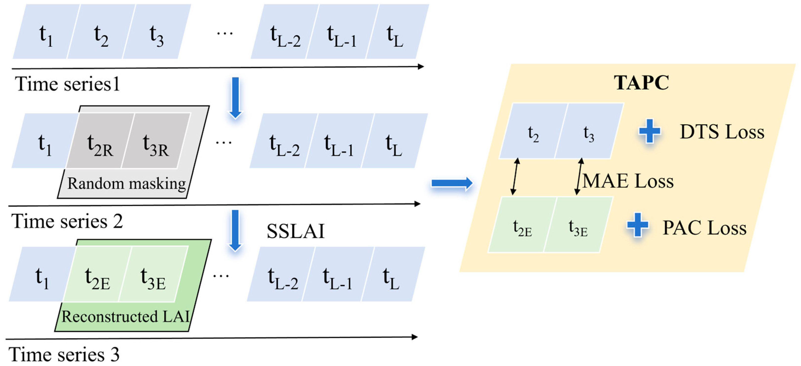
(4) To fit pixel-scale vegetation growth rhythms without vegetation type classification, a novel temporally adaptive phenological constraint loss (TAPC) function was proposed. This composite loss, consisting of Mean Absolute Error (MAE) loss, dynamic temporal smoothing (DTS) loss, and peak adaptive constraint (PAC) loss, ensures overall reconstruction accuracy via MAE loss, restricts non-physiological abrupt changes with DTS loss using pixel-adaptive LAI first-order difference slope thresholds, and penalizes deviant predicted peaks with PAC loss based on pixel-wise historical LAI 95th percentiles and ±15% deviation weighted penalties. This loss function effectively guarantees the ecological rationality of the reconstructed LAI, which can serve as high-quality data support for terrestrial ecosystem and land surface process research.

This paper is organized as follows. Section 2 describes the datasets, and Section 3 details the SSLAI framework, experimental setup, and comparison methods. Section 4 presents the experimental results. Section 5 discusses limitations and future improvements, and Section 6 summarizes the conclusions.

2. Materials

2.1. Study Area

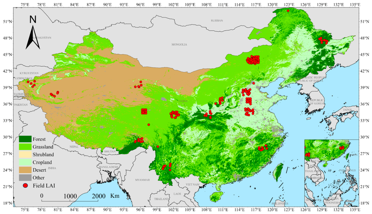
This study selected China as the study area, spanning 73.55–135.08° E and 3.85–53.55° N. With complex terrain, diverse temperate, subtropical, tropical, arid, and alpine climates, as well as varied forests, grasslands, croplands, shrublands, and desert vegetation, it exhibits significant spatial heterogeneity and distinct seasonal vegetation dynamics. Thus, China is ideal and representative for evaluating 500 m spatial resolution LAI product performance and validating spatio-temporal gap-filling algorithms. Figure 1 is from the 2024 MODIS land cover product (MCD12Q1.061) [30], where red dots represent the field LAI used in this study.

2.2. Data Description and Processing

(1)

MODIS LAI

The MODIS LAI product (MOD15A2H) has 500 m spatial resolution and 8-day temporal resolution. Its retrieval algorithm is based on a three-dimensional radiative transfer model, with biome-specific lookup tables matching satellite-observed surface reflectance [31].

(2)

Meteorological Data

CTP, CSSRD, and AT2 were from the ERA5-Land dataset (hourly, 0.1° spatial resolution) [32]. These data were aggregated to 8-day intervals and resampled to 500 m to match MODIS LAI’s spatio-temporal resolution, as they are critical for vegetation phenology and LAI dynamics. Detailed information is presented in

Table 1. Overview of multi-source remote sensing and geospatial datasets used in this study.

Dataset	Variable	Spatial Resolution	Temporal Resolution	Temporal Coverage	Data Provider	Access Link
MOD15A2H	LAI	500 m	8 days	2015–2025	NASA	https://earthdata.nasa.gov/ (Accessed on 13 February 2026)
ERA5-Land	CTP	0.1°	Hourly	2015–2025	ECMWF	https://cds.climate.copernicus.eu (Accessed on 15 February 2026)
	CSSRD
	AT2
SRTM DEM	DEM	90 m	-	2018	NASA	https://srtm.csi.cgiar.org/ (Accessed on 11 February 2026)
	Slope
	Aspect
MOD13A1	NDVI	500 m	16 days	2015–2025	NASA	https://earthdata.nasa.gov/ (Accessed on 2 March 2026)

.

(3)

Topographic data

NASA’s Shuttle Radar Topography Mission (SRTM) 90 m digital elevation model (DEM) data were acquired for the study area; slope and aspect parameters were derived from the DEM and then resampled from 90 m to 500 m to ensure spatial consistency with other datasets used in this study [33].

(4)

NDVI

The 500 m MODIS NDVI data were obtained from the MOD13A1 Collection 6.1 product with a 16-day composite interval [34]. To match the 8-day temporal resolution of the MODIS LAI product, the NDVI data were resampled to an 8-day interval.

(5)

Field LAI Measurements

To validate SSLAI, field LAI measurements were collected independently from 2018 to 2025. The sampling sites systematically cover five dominant vegetation types and five major climate zones, representing the climatic and ecological gradients from south to north and west to east across China with a stratified and representative sampling design. All used a calibrated LAI-2200 Plant Canopy Analyzer (Li-Cor, Lincoln, NE, USA), a recognized remote sensing validation tool. Standardized procedures ensured data reliability: measurements were taken 06:00–09:00 or 16:00–18:00 to avoid solar interference; 5 repeats per site (≥1 m from edges), mean as LAI; outliers (±2 standard deviations) removed; LAI-2200 annually calibrated and weekly field-checked. Sampling ensured spatial representativeness: seasonal measurements synchronized with MODIS 8-day composites; long-term sites (e.g., Xilingol Grassland) measured annually. Details are in Appendix A 

Table A1. Basic information on field LAI sites used in this study.

Ecosystem Type	Region	Coordinates	Year	No. of Sites
Forest	Northeast China (Lesser Khingan Range)	47.00–48.00° N, 129.00–130.00° E	2018–2025	10
Forest	Southwest Yunnan mountainous area	24.00–25.00° N, 100.00–101.00° E	2018–2025	10
Forest	Qinling Mountains	33.00–34.00° N, 108.00–109.00° E	2018–2025	10
Forest	Motou	29.00–30.00° N, 95.00–96.00° E	2018–2025	10
Forest	Wuyi Mountains	27.00–28.00° N, 118.00–119.00° E	2018–2025	10
Forest	Greater Khingan Range	52.97° N, 122.83° E	2020	1
Grassland	Eastern Qinghai-Tibet Plateau	34.00–35.00° N, 96.00–97.00° E	2018	10
Grassland	Eastern Qinghai-Tibet Plateau	33.00–34.00° N, 102.00–103.00° E	2018–2025	30
Grassland	Xilinhot	43.00–44.00° N, 116.00–117.00° E	2018–2025	30
Grassland	Baima Snow Mountain NR, Diqing	28.28° N, 99.15° E	2018	1
Grassland	Xilingol	43.42–44.67° N, 115.50–117.17° E	2019–2023	30
Grassland	Eastern Qinghai-Tibet Plateau	32.25° N, 97.50° E	2022	1
Shrubland	Arid region of Northwest China (Jiuquan)	39.00–40.00° N, 95.00–96.00° E	2018–2025	8
Shrubland	Loess Plateau (Yan’an)	36.00–37.00° N, 110.00–111.00° E	2018–2025	7
Cropland	North China Plain (Shijiazhuang)	38.00–39.00° N, 115.00–116.00° E	2018–2025	20
Cropland	Huang-Huai-Hai Plain (Shangqiu)	34.00–35.00° N, 115.00–116.00° E	2018–2025	20
Cropland	North China Plain	36.00–37.00° N, 115.00–116.00° E	2018	10
Cropland	Langfang, Hebei	39.78° N, 116.58° E	2019	1
Cropland	North China Plain	37.87° N, 115.42° E	2020	1
Desert	Hotan region	37.00–38.00° N, 80.00–81.00° E	2018–2025	5
Desert	Kashgar region	39.00–40.00° N, 76.00–77.00° E	2018–2025	5

.

(6)

Data preprocessing

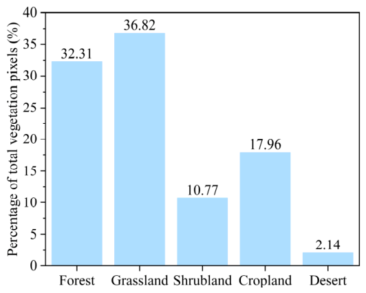
MOD15A2H Version 6.1 from 2015 to 2025 was divided into three subsets: (1) pretraining from 2015 to 2017, which covers complete climatic cycles, with representative vegetation distribution shown in Figure 2, including grassland accounting for 36.82%, forest for 32.31%, cropland for 17.96%, shrubland for 10.77%, and desert for 2.14%; (2) validation in 2018 for hyperparameter optimization and overfitting suppression; (3) testing from 2019 to 2025 for independent long-term reconstruction and adaptability evaluation under extreme events such as drought.

Then, 32 × 32 pixel patches were generated: 114,922 pre-training and 38,189 validation samples. An 8-bit quality control (QC) band was used for masking, with only unsaturated data retrieved by the main algorithm (0 ≤ QC < 32) retained [35]. Data with 32 ≤ QC < 64 indicated saturation in the main inversion algorithm, while 64 ≤ QC < 128 denoted main algorithm failure with backup algorithm application. Data with QC ≥ 128 corresponded to unretrieved or unprocessed pixels. These low-quality data categories were excluded [36], ensuring the training dataset was of high quality and noise-free.

3. Methods

3.1. Overall Framework

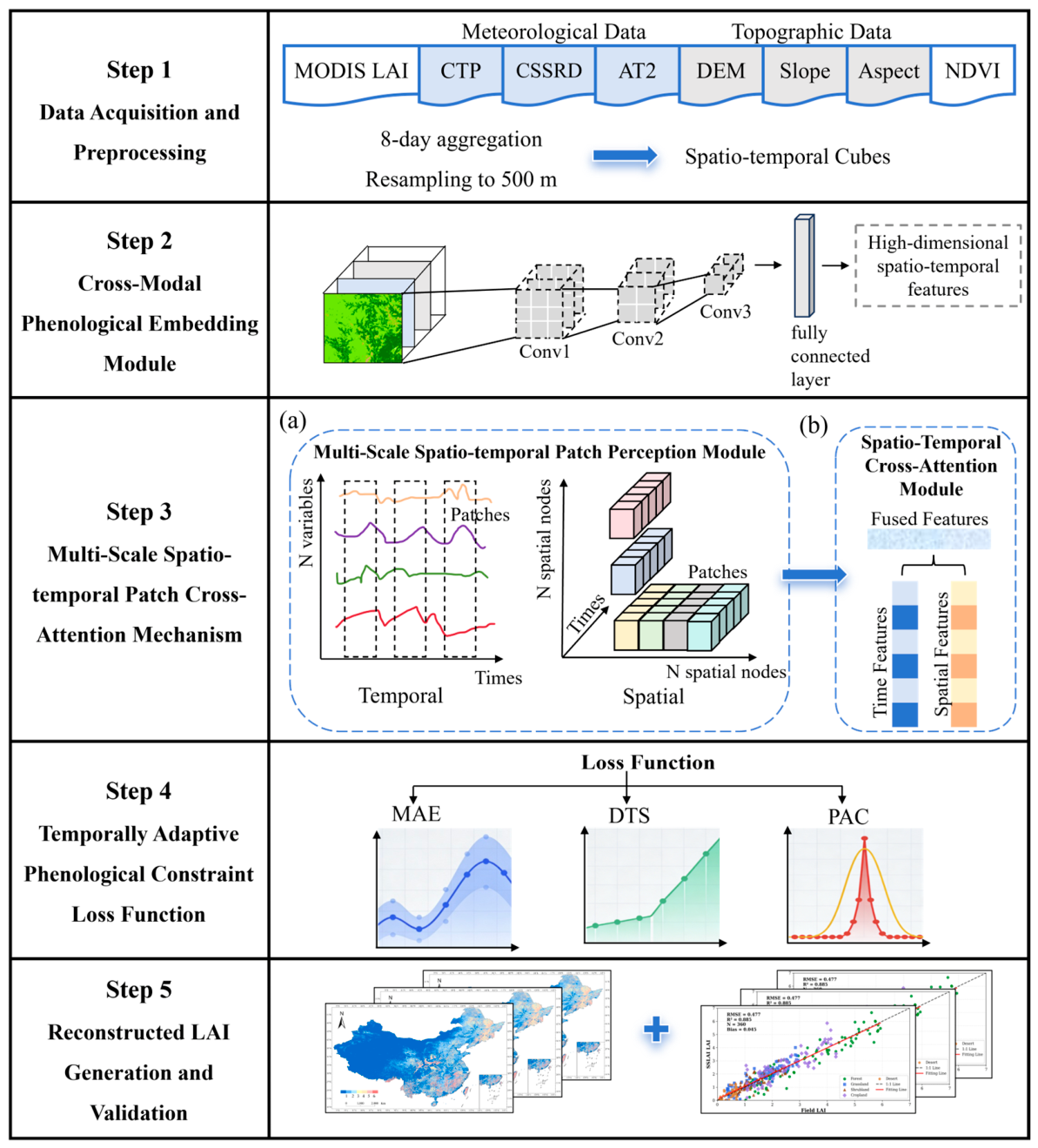
To address the extensive spatio-temporal gaps in MODIS LAI products caused by cloud contamination and sensor noise, the SSLAI framework was proposed to support high-quality terrestrial vegetation monitoring. First, a CPE fuses MODIS LAI time series and environmental covariates to capture the inherent coupling between vegetation growth and environmental conditions. Second, a multi-scale spatio-temporal patch cross-attention mechanism extracts multi-scale spatial and temporal features, enhancing phenological dynamics capture across heterogeneous landscapes. Third, a spatio-temporal cross-attention module models long-range LAI time series dependencies, overcoming deficiencies in spatio-temporal feature mining for continuous vegetation monitoring. Fourth, a TAPC function—integrating MAE, DTS, and PAC losses—suppresses non-physiological fluctuations and unrealistic peaks, ensuring consistency between reconstructed LAI and actual vegetation growth rhythms. Lastly, a self-supervised masking strategy masks high-quality LAI values during training, enabling feature learning from unlabeled data and improving generalization for large-scale MODIS LAI reconstruction. As shown in Figure 3, all modules collaborate to form an end-to-end framework boosting reconstructed LAI accuracy for terrestrial ecosystem research.

3.2. Cross-Modal Phenological Embedding Module

LAI dynamics are closely linked to environmental constraints, as precipitation, solar radiation, and temperature directly regulate vegetation growth and phenological transitions [37]. Integrating these key features is critical for improving the physical interpretability and reconstruction accuracy of MODIS LAI time series, especially for filling gaps caused by extreme climate events or critical phenological periods.

To effectively fuse heterogeneous LAI and meteorological data, a lightweight 3D Convolutional Neural Network (3D CNN) was designed as the module core. Its architecture consists of three 3D convolutional layers with a 3 × 3 × 3 convolution kernel size, two max-pooling layers, and one fully connected layer, with ReLU activation functions to introduce non-linearity and enhance feature expression. Inputs are spatio-temporal cubes, denoted as $X_t^i\in R^{H\ast W\ast B}$, where H (height) and W (width) are 32 × 32 pixels (Section 2.2), t denotes MODIS 8-day composite periods, and B = 8 (MODIS LAI, CTP, CSSRD, AT2, DEM, slope, aspect, and NDVI). Each cube $X_t^i$ integrates LAI and climate driver information over a 32 × 32-pixel spatial area and time t. The value at position $\left(\mathrm{x},y,z\right)$ in the $j$-th feature map of the $i$-th convolutional layer is calculated as [38]:

$$f_{ij}^{xyz}=\sigma \left(b_{ij}+{\displaystyle \sum }_m{\displaystyle {\displaystyle \sum }_{a=0}^{A_i-1}}{\displaystyle {\displaystyle \sum }_{b=0}^{B_i-1}}{\displaystyle {\displaystyle \sum }_{c=0}^{C_i-1}}{w}_{ijm}^{abc}{m}_{(i-1)m}^{(x+a)(y+b)(z+c)}\right)$$

(1)

where $\sigma \left(\cdot \right)$ denotes the activation function (ReLU); $b_{ij}$ and $w_{ijm}^{abc}$ represent the weights and bias parameter; $m$ indexes over the input feature maps from the $\left(i-1\right)$ layer; $m_{(i-1)m}^{(x+a)(y+b)(z+c)}$ denotes the input feature value at the corresponding receptive field location; and $A_i$, $B_i$, and $C_i$ represent the height, width, and depth of the 3D convolutional kernel, respectively. Following feature extraction through the 3D CNN, the original input cube $X^i\in R^{H\ast W\ast B\ast T}$ is transformed into a high-dimensional temporal feature representation$\left\{M_{(3d)}^1\cdot \cdot \cdot M_{(3d)}^N\right\}\in R^{N\times T\times d}$; where $N$ is the number of spatial units, $T$ is the temporal dimension, and $d$ is the final embedding dimension produced by the fully connected layer.

3.3. Multi-Scale Spatio-Temporal Patch Cross-Attention Mechanism

3.3.1. Multi-Scale Spatio-Temporal Patch Perception Module (MSTPP)

Vegetation LAI dynamics are significantly affected by seasonal rhythms and spatial heterogeneity [39,40]. This study adopted a patch-based Transformer framework, inspired by Natural Language Processing (NLP) semantic modeling [41,42,43], to capture long-range dependencies with reduced attention complexity [44], while multi-band data are processed channel-independently to enhance spatio-temporal feature interpretability.

(1)

Temporal Patch Feature Learning across Different Growth Cycles

Existing Transformer-based temporal feature extraction methods are limited to a single/fixed time scale, making it hard to adapt to vegetation phenotypic variations across monthly, seasonal, and annual cycles. This module achieves collaborative feature learning at three scales (month, season, and year) through multi-scale temporal patch division and multi-head attention.

Let the time series of the b-th input band (b = 1, 2, ..., 4) be denoted as $X_b\in R^{T\times 1}$, where T denotes the total number of time steps (unit: day). Non-overlapping sliding windows are adopted for patch division, with window length P and stride S (S = P to ensure non-overlapping). Given the 8-day temporal resolution of the dataset, three strides are defined for the corresponding growth cycle scales: monthly scale: S₁ = 4; seasonal scale: S₂ = 12; and annual scale: S₃ = 46, corresponding to typical vegetation growth cycles at monthly, seasonal, and annual scales, respectively. The number of patches generated at each scale is given by $N_s=⌊{\displaystyle \frac{(T-P_s)}{S_s}}⌋+1$ (s = 1, 2, 3), $P_{\mathrm{s}}=S_s$, where $N_s$ represents the total number of patches at the s-th scale. The resulting temporal patch sequence is $X_{b,s}=\left\{x_{b,s,1},x_{b,s,2},\dots ,x_{b,s,N_s}\right\}$, in which each individual patch is denoted as $x_{b,s,i}\in R^{P_s\times 1}$. For the patch sequence at each scale, linear projection and positional encoding are performed as follows [45]:

$$Z_{b,s,i}=W_{p,s}\cdot x_{b,s,i}+P{E}_{s,i}$$

(2)

where $W_{p,s}\in R^{D\times P_s}$ is the projection matrix at the s-th scale (D is the feature dimension); and $P{E}_{s,i}\in R^D$ denotes the sine-cosine positional encoding of the i-th patch. Multi-scale temporal features are aggregated via the multi-head attention mechanism:

$$\mathrm{MultiHead}(Z_{b,s})=\mathrm{Concat}({\mathrm{head}}_1,{\mathrm{head}}_2,\dots ,{\mathrm{head}}_h)\cdot W^O$$

(3)

where each attention head is computed as:

$${\mathrm{head}}_k=\mathrm{Softmax}\left({\displaystyle \frac{Q_k·K_k^T}{\sqrt{d_k}}}\right)\cdot V_k$$

(4)

where $Q_k=Z_{b,s}\cdot W_q^k,K_k=Z_{b,s}\cdot W_k^k,V_k=Z_{b,s}\cdot W_k^k$ denote the query, key, and value matrices, respectively; $W_q^k,W_k^k,W_v^k\in R^{D/h\times D}$ is the parameter matrix of the k-th head; $d_k=D/h$ is the feature dimension of each attention head; and $W^O\in R^{D\times D}$ is the output projection matrix. Lastly, the temporal features from the three scales are concatenated to obtain the global temporal feature $F_t\in R^{D\times 3}$.

(2)

Spatial Patch Feature Learning across Different Spatial Scales

Different from temporal feature learning, the spatial module treats image pixels as discrete spatial nodes and captures geographical heterogeneity via multi-scale spatial aggregation. We construct three spatial scales by average pooling of 2 × 2, 3 × 3, and 4 × 4 neighboring pixels, respectively, to generate multi-scale spatial units. Multi-scale spatial pooling (2 × 2, 3 × 3, and 4 × 4) was used to capture spatial heterogeneity at different levels, from local pixels to regional patterns. This design helps the model adapt to fragmented farmland, continuous grasslands, and mountainous forests across China. The time series of each spatial unit is then linearly projected and sent to the spatial multi-head attention module with spatial positional encoding. Following the same attention mechanism as the temporal module, the final output is the global spatial feature.

3.3.2. Spatio-Temporal Cross-Attention Module (STCA)

For deep temporal–spatial feature interaction, a cross-attention mechanism was adopted for bidirectional fusion. F_t (global temporal feature) serves as Query, F_s (global spatial feature) as Key and Value for spatial-guided temporal attention; F_s as Query, F_t as Key and Value for temporal-guided spatial attention. The spatio-temporal joint feature is finally obtained via weighted fusion. The detailed computation is as follows:

Spatial-guided temporal attention:

$${\mathrm{Att}}_{s\to t}=\mathrm{Softmax}\left({\displaystyle \frac{F_t\cdot F_s^T}{\sqrt{D}}}\right)\cdot F_s$$

(5)

Temporal-guided spatial attention:

$${\mathrm{Att}}_{t\to s}=\mathrm{Softmax}\left({\displaystyle \frac{F_s\cdot F_t^T}{\sqrt{D}}}\right)\cdot F_t$$

(6)

Spatio-temporal features are fused by element-wise addition:

$$F_{ts}=At{t}_{s\to t}+At{t}_{t\to s}$$

(7)

The fused feature $F_{ts}\in R^D$ is fed into a two-layer fully connected network to output the LAI reconstruction result. This two-layer structure is selected to ensure efficient feature mapping and reduce the risk of overfitting.

$$L\widehat{A}I(t)=W_2\cdot \mathrm{ReLU}(W_1\cdot F_{ts}+b_1)+b_2$$

(8)

where $W_1\in R^{D/2\times D}$ and $W_2\in R^{1\times D/2}$ are weight matrices, and b₁ and b₂ are bias terms.

3.4. Temporally Adaptive Phenological Constraint Loss Function

To ensure the reconstructed LAI conforms to the natural laws of vegetation growth, a Temporally Adaptive Phenological Constraint (TAPC) loss is proposed, which consists of MAE, DTS, and PAC components. MAE ensures reconstruction accuracy by minimizing the absolute deviation between the reconstructed LAI and the original LAI. DTS constrains non-physiological abrupt changes in LAI via a pixel-adaptive threshold derived from the first-order difference slope of the LAI time series, penalizing violations of vegetation growth temporal continuity. PAC uses the 95th percentile of each pixel’s historical LAI as a reference, penalizing reconstructed peaks that deviate from this reference by ±15% to match the inherent growth characteristics of each pixel. The total loss function is formulated as follows:

$$L_{total}=L_{MAE}+\alpha \cdot L_{DTS}+\beta \cdot L_{PAC}$$

(9)

where α and β are the weight coefficients for DTS and PAC, respectively. The MAE loss is defined as follows:

$$L_{MAE}={\displaystyle \frac{1}{N}}{\displaystyle \sum \begin{array}{c}N\\ i=1\end{array}}\left|L\widehat{A}{I}_i-LA{I}_i\right|$$

(10)

where N is the number of temporal samples per pixel; $L\widehat{A}{I}_i$ denotes the reconstructed LAI values; and $LA{I}_i$ represents the original LAI values before masking. The DTS loss is computed as follows:

$$L_{DTS}={\displaystyle \sum \begin{array}{c}T-1\\ t=1\end{array}\left|\left(L\widehat{A}{I}_{t+1}-L\widehat{A}{I}_t\right)-{\delta }_i^{th}\right|}\cdot I\left(\left|L\widehat{A}{I}_{t+1}-L\widehat{A}{I}_t\right|>{\delta }_i^{th}\right)$$

(11)

where t denotes the time step; ${\delta }_i^{th}$ is the pixel-adaptive threshold for the i-th pixel; and $I(\cdot )$ is an indicator function that equals 1 if the condition holds and 0 otherwise. The PAC loss is expressed as:

$$L_{PAC}={\displaystyle {\sum }_{p=1}^P\left|L\widehat{A}{I}_p-LA{I}_i^{95\%}\right|}\cdot I\left(\left|{\displaystyle \frac{L\widehat{A}{I}_p-LA{I}_i^{95\%}}{LA{I}_i^{95\%}}}\right|>0.15\right)$$

(12)

where P is the number of predicted peak points for the i-th pixel; and $LA{I}_i^{95\%}$ is the 95th percentile of the historical LAI values for the i-th pixel.

3.5. Adaptive Self-Supervised Masking Strategy

To reduce dependence on labeled data and improve the generalization performance for complex vegetation phenology in MODIS LAI reconstruction, an adaptive self-supervised masking strategy is proposed (Figure 4). High-quality LAI values are randomly masked as missing (denoted as 0) for each pixel-level MODIS LAI time series during training (t_2R, t_3R in Figure 4). The model reconstructs masked LAI values (i.e., t_2E, t_3E in Figure 4) using two contextual features: (1) vegetation-growth-correlated environmental covariate features (Section 3.2), fused to improve LAI predictability under extreme phenological events; (2) spatio-temporal contextual features from unmasked LAI via the multi-scale spatio-temporal patch cross-attention mechanism (Section 3.3). Lastly, the TAPC is calculated to constrain the reconstruction results and ensure the rationality of the reconstructed LAI values.

3.6. Experimental Settings and Evaluation Metrics

All traditional gap-filling and deep learning methods were implemented using PyTorch 2.1.0 for a unified experimental environment. For the SSLAI, the initial learning rate was set to 1 × 10⁻⁴, with 200 training epochs. To ensure experimental fairness, all deep learning models underwent hyperparameter optimization via Bayesian optimization (learning rate: 1 × 10⁻⁴–1 × 10⁻²; batch size: 16, 32, 64; dropout rate: 0.1–0.5). They adopted the Adam optimizer (weight decay 1 × 10⁻⁵), with early stopping (patience = 20) to prevent overfitting. Traditional MODIS LAI gap-filling methods (DL, SG, and DTS) used 5-fold cross-validation and grid search for tuning: DL optimized logical thresholds (0.05–0.5) and iterations (50–500); SG optimized the Savitzky–Golay window size (3, 5, 7, 9) and polynomial order (1–3); and DTS optimized the temporal smoothing coefficient (0.1–0.8) and abrupt change threshold (0.01–0.1). All experiments were conducted on a computational platform with Intel Core i9-13900K CPU (64-bit), NVIDIA GeForce RTX 4090 GPU, and CUDA Toolkit v12.6.37.

In this study, three quantitative metrics were adopted to evaluate the performance of the proposed framework: root mean square error (RMSE), coefficient of determination (R²), and bias. Their definitions are as follows:

$$RMSE=\sqrt{{\displaystyle \frac{1}{N}}{\displaystyle {\displaystyle \sum }_{i=1}^N}{(r_i-y_i)}^2}$$

(13)

$$R^2=1-{\displaystyle {\displaystyle \sum }_{i=1}^N}{(r_i-y_i)}^2/{\displaystyle {\displaystyle \sum }_{i=1}^N}{(r_i-\overline{y})}^2$$

(14)

$$Bias={\displaystyle \frac{1}{N}}{\displaystyle {\displaystyle \sum }_{i=1}^N}(r_i-y_i)$$

(15)

where N denotes the number of reconstructed data points; $y_i$ and $r_i$ represent the high-quality LAI before masking and the reconstructed LAI, respectively; and $\overline{y}$ is the mean value of $y_i$.

To evaluate model complexity and computational efficiency, two metrics were adopted: the number of model parameters (Params) and giga floating-point operations (GFLOPs) [46]. Params represents the total learnable weights, while GFLOPs quantify the computational workload for model inference. Lower GFLOPs indicate faster inference and lower resource consumption. Both indicators were calculated using the THOP library through a single forward pass of the PyTorch model.

3.7. Comparison Methods

Seven methods, both conventional gap-filling algorithms and state-of-the-art deep learning models, were adopted to evaluate the effectiveness of the proposed SSLAI for missing MODIS LAI reconstruction.

(1) DL (Double Logistic algorithm) [47]: A conventional logic-driven gap-filling method for MODIS LAI product post-processing.

(2) SG (Savitzky–Golay filter) [48]: A temporal smoothing method for satellite vegetation index reconstruction, filling LAI gaps via local polynomial fitting of time series segments.

(3) DTS (Dynamic Temporal Smoothing algorithm) [49]: An improved gap-filling method based on temporal constraints, suppressing non-physiological LAI abrupt changes with an adaptive coefficient.

(4) Bi-LSTM [19]: A recurrent model for time-series modeling capturing bidirectional LAI sequence dependencies and widely used for Landsat time-series missing data reconstruction.

(5) MBPNN [7]: A multi-branch fully connected model for remote sensing vegetation index reconstruction, integrating meteorological covariates and LAI features to improve filling accuracy.

(6) EDCSTFN [50]: A framework fusing SAR and photosynthetic data via the 2D CNN-Transformer, enhancing LAI reconstruction accuracy in cloudy regions with enhanced spatial-temporal fusion.

(7) STINet [35]: A Transformer-based method capturing long-range LAI time series spatio-temporal dependencies to recover cloud-contaminated missing values and generate high-quality MODIS LAI products.

4. Results

4.1. Benchmark Evaluation of Competing Methods for LAI Reconstruction

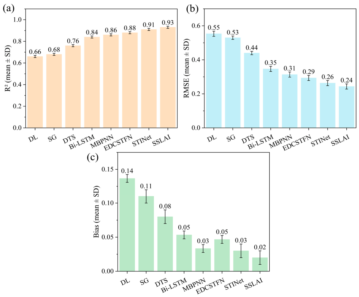
To verify the superiority of the proposed SSLAI in 500 m spatial resolution MODIS LAI reconstruction across China, eight methods were evaluated. Performance was quantified using R², RMSE, and bias, with the results shown in Figure 5. Error bars represent the standard deviation (SD) for multi-year (2019–2025) datasets. Conventional methods (DL, SG, and DTS) performed the worst, with R² values below 0.8. In contrast, other deep learning-based models achieved better performance, with RMSE values below 0.4. Notably, the proposed SSLAI achieved the highest R² of 0.93, the lowest RMSE of 0.24, and the lowest bias of 0.02. For further evaluation of computational efficiency, model Params and GFLOPs were compared, as shown in

Table 2. Model complexity and computational cost. Params (M) denote millions of trainable parameters. GFLOPs denote billions of floating-point operations.

Method	Params (M)	GFLOPs
Bi-LSTM	2.65	1.82
MBPNN	0.15	0.08
EDCSTFN	6.82	4.35
STINet	5.17	3.29
SSLAI	3.42	2.57

. Since conventional statistical methods do not involve trainable parameters, only deep learning-based approaches were included in this comparison. SSLAI achieves a favorable balance between accuracy and computational cost, with moderate Params of 3.42 M and GFLOPs of 2.57. Therefore, SSLAI exhibits competitive overall performance across various evaluation metrics and achieves satisfactory comprehensive results, demonstrating its promising effectiveness and robustness for large-scale, high-quality LAI reconstruction.

4.2. Temporal Trajectory Comparison of Competing Methods over Three Typical Ecological Landscapes

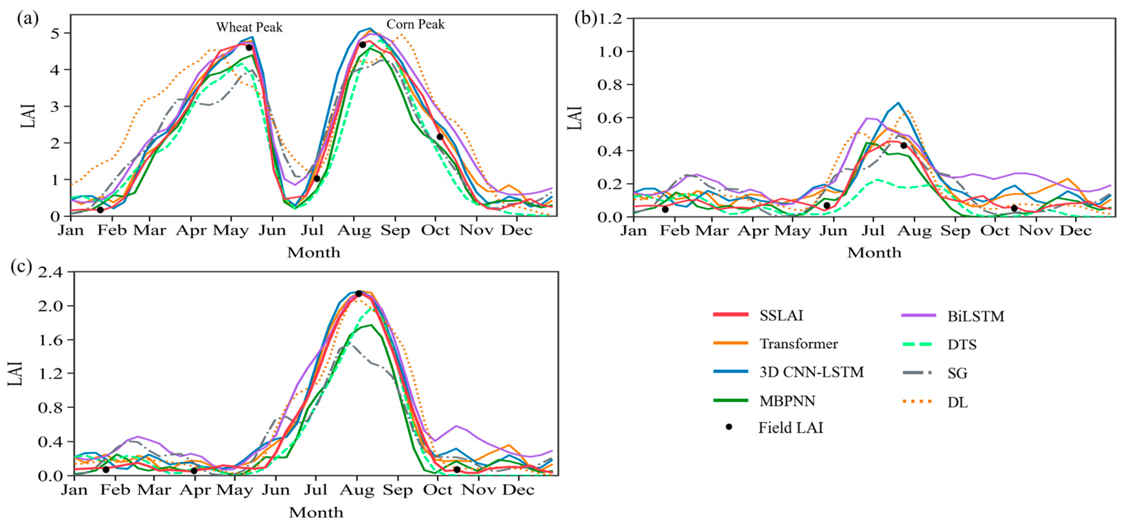
To complement quantitative evaluation and validate the model’s ability to capture fine-scale phenological dynamics under climatic stress, three test sites were selected: (1) Langfang, Hebei (39.78° N, 116.58° E), North China Plain, typical winter wheat–summer maize rotation; 2019 was selected for severe spring drought during winter wheat jointing; (2) Baima Snow Mountain National Nature Reserve, Deqin, Yunnan (28.28° N, 99.15° E), alpine meadow; 2018 study period had exceptional midsummer drought (July–August), ideal for testing cold-region water stress sensitivity; (3) the site is located in the Northern Greater Khingan Mountains (52.97° N, 122.83° E). This 2020 study area is a cold-temperate deciduous coniferous forest with distinct seasonality and minimal human disturbance. This site serves as a baseline control for comparison with the drought-stressed sites mentioned above.

Figure 6 compares the LAI time series from eight models with field LAI at three sites. In Langfang in 2019 (Figure 6a), the cropping system exhibited a bimodal LAI pattern. Conventional methods (DL, SG, and DTS) underestimate winter wheat LAI peaks and predict earlier emergence. In contrast, SSLAI accurately tracks both crop LAI peaks, consistent with field measurements. In the Diqing alpine meadow in 2018 (Figure 6b), most models, particularly Bi-LSTM and EDCSTFN, overestimate July–August LAI due to low temperatures and midsummer drought. SSLAI integrates meteorological stress signals, producing a curve that reflects drought-suppressed growth peaks. In the northern Greater Khingan Mountains in 2020 (Figure 6c), all methods capture unimodal phenology. SSLAI outperforms other models in senescence reconstruction, avoiding over-smoothing in SG and irregular fluctuations in Bi-LSTM.

4.3. Ablation Study of Key Functional Modules and Loss Function

To verify the effectiveness and necessity of each key component, a step-by-step ablation study was conducted on the test set. The baseline model adopted a basic encoder without customized modules, achieving an R² of 0.76, an RMSE of 0.45, and a bias of 0.18. As shown in

Table 3. Ablation study results of the SSLAI on the test set (2019–2025). Metrics are presented as the mean ± SD over seven years. The check mark (√) in each row indicates the corresponding module is included. The best result is highlighted in bold. ↑ denotes that higher values are preferable. ↓ denotes that lower values are preferable.

		Strategy
Baseline	CPE	MSTPP	STCA	TAPC	R2 (Mean ± SD) ↑	RMSE (Mean ± SD) ↓	Bias (Mean ± SD )↓
√					0.76 ± 0.04	0.45 ± 0.05	0.18 ± 0.04
√	√				0.83 ± 0.03	0.37 ± 0.04	0.12 ± 0.03
√	√	√			0.87 ± 0.02	0.32 ± 0.03	0.09 ± 0.03
√	√	√	√		0.90 ± 0.01	0.28 ± 0.02	0.06 ± 0.02
√	√	√	√	√	0.93 ± 0.01	0.24 ± 0.02	0.02 ± 0.01

, with the sequential addition of the four modules, the RMSE gradually decreased while the R² increased continuously. The full SSLAI model achieved an R² 22.37% higher, an RMSE 46.67% lower, and a bias 88.89% lower than the baseline model.

Table 4. Ablation experiment results of the TAPC loss function. Metrics are presented as the mean ± SD over seven years. The check mark (√) in each row indicates the corresponding component is included. The best result is highlighted in bold. ↑ denotes that higher values are preferable. ↓ denotes that lower values are preferable.

	TAPC
MAE	DTS	PAC	R2 (Mean ± SD) ↑	RMSE (Mean ± SD) ↓	Bias (Mean ± SD) ↓
√			0.83 ± 0.03	0.36 ± 0.04	0.07 ± 0.02
√	√		0.89 ± 0.02	0.29 ± 0.03	0.04 ± 0.01
√	√	√	0.93 ± 0.01	0.24 ± 0.02	0.02 ± 0.01

shows the performance of different TAPC loss combinations. Removing any of MAE, DTS, or PAC decreased the R² and increased the RMSE. The complete SSLAI with four components achieved the best performance, with an R² of 0.93, an RMSE of 0.24, and a bias of 0.02, validating the rationality and superiority of the proposed framework.

4.4. Validation Against Field LAI Measurements

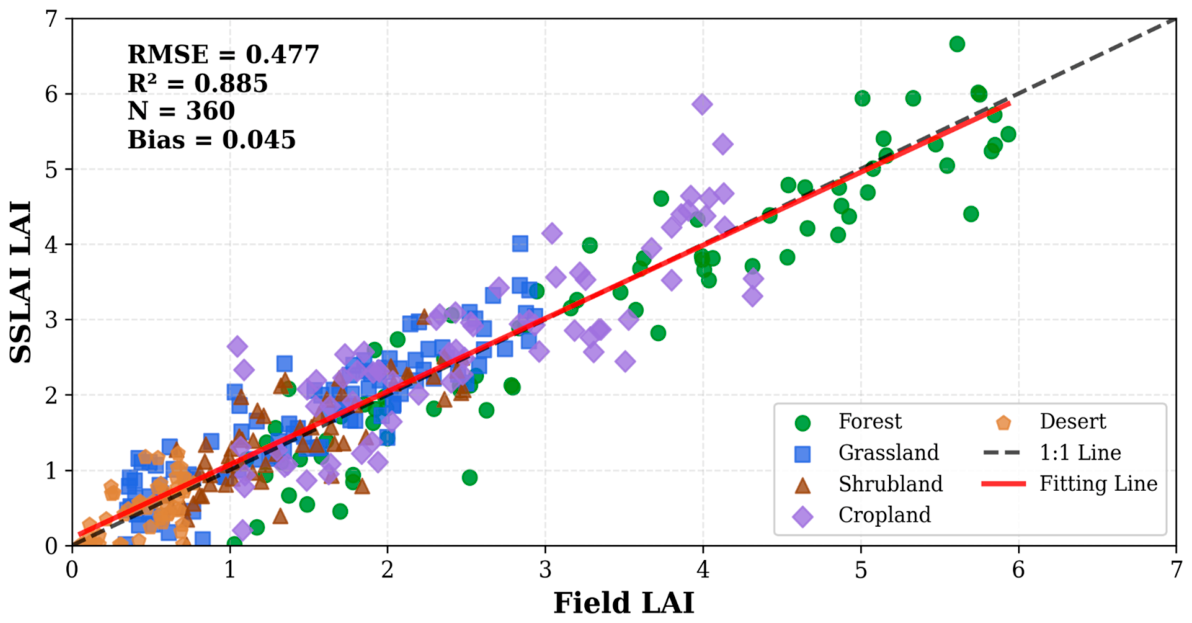
To verify the SSLAI’s accuracy and applicability, comprehensive validation was performed using 2018–2025 field LAI data from five typical Chinese vegetation types (Figure 7). The SSLAI model achieved favorable accuracy, with an R² of 0.885, an RMSE of 0.477, and a bias of 0.045. The field dataset included 175 representative sampling points covering all ecozones listed in Table A1. Specifically, 50 forest sites are located in the Lesser Khingan Mountains, southwestern Yunnan, Qinling Mountains, Motuo, and Wuyi Mountain; 60 grassland sites are in the eastern Qinghai-Tibet Plateau alpine meadow and Xilinhot grassland; 15 shrubland sites are in the Jiuquan arid region and Yan’an Loess Plateau; 40 cropland sites are in Shijiazhuang and Shangqiu; and 10 desert sites are in Hotan and Kashgar. The experimental results are presented in

Table 5. Validation between reconstructed LAI and field LAI across geographic regions and vegetation types.

Study Area/Vegetation Type	R2	RMSE	Bias
Forest	0.918	0.409	0.040
Northeast China (Lesser Khingan Range)	0.921	0.402	0.038
Southwestern Yunnan Mountainous Area	0.918	0.415	0.042
Qinling Mountains	0.925	0.398	0.035
Motuo	0.912	0.421	0.045
Wuyi Mountains	0.915	0.408	0.040
Grassland	0.860	0.518	0.053
Eastern Qinghai–Tibet Plateau	0.862	0.512	0.052
Xilinhot	0.858	0.525	0.055
Shrubland	0.872	0.485	0.048
Arid region of Northwest China (Jiuquan)	0.869	0.483	0.047
Loess Plateau (Yan’an)	0.872	0.485	0.048
Cropland	0.893	0.466	0.043
North China Plain (Shijiazhuang)	0.895	0.462	0.042
Huang-Huai-Hai Plain (Shangqiu)	0.892	0.470	0.044
Desert	0.782	0.658	0.073
Hotan Surrounding Area	0.778	0.665	0.075
Kashgar Surrounding Area	0.782	0.658	0.073

. All vegetation types and their corresponding study areas yielded reliable reconstruction accuracy, with the R² higher than 0.77. These results were highly consistent with the overall validation performance. Overall, the SSLAI product exhibited good agreement with field-measured LAI.

4.5. Inter-Product Comparison and Vegetation-Specific Accuracy of the Reconstructed LAI

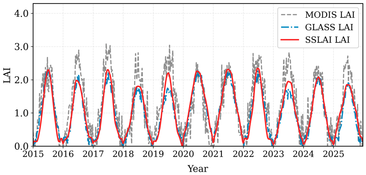
To evaluate SSLAI LAI’s long-term temporal consistency, a representative site in the Xilingol Grassland (43.90° N, 116.70° E) was selected for inter-product comparison. This typical northern Chinese temperate grassland has distinct phenology and minimal mixed vegetation, avoiding complex land cover interference. Figure 8 compares MODIS, GLASS, and SSLAI LAI time series (2015–2025), covering the full MODIS Collection 6.1 record for sensor consistency [51,52]. MODIS LAI shows frequent fluctuations and abnormal drops from aerosol pollution and sensor noise; GLASS LAI is smoother but often underestimates peaks. SSLAI maintains excellent long-term smoothness and interannual stability, mitigating GLASS’s underestimation and MODIS’s instability for reliable long-term reconstruction.

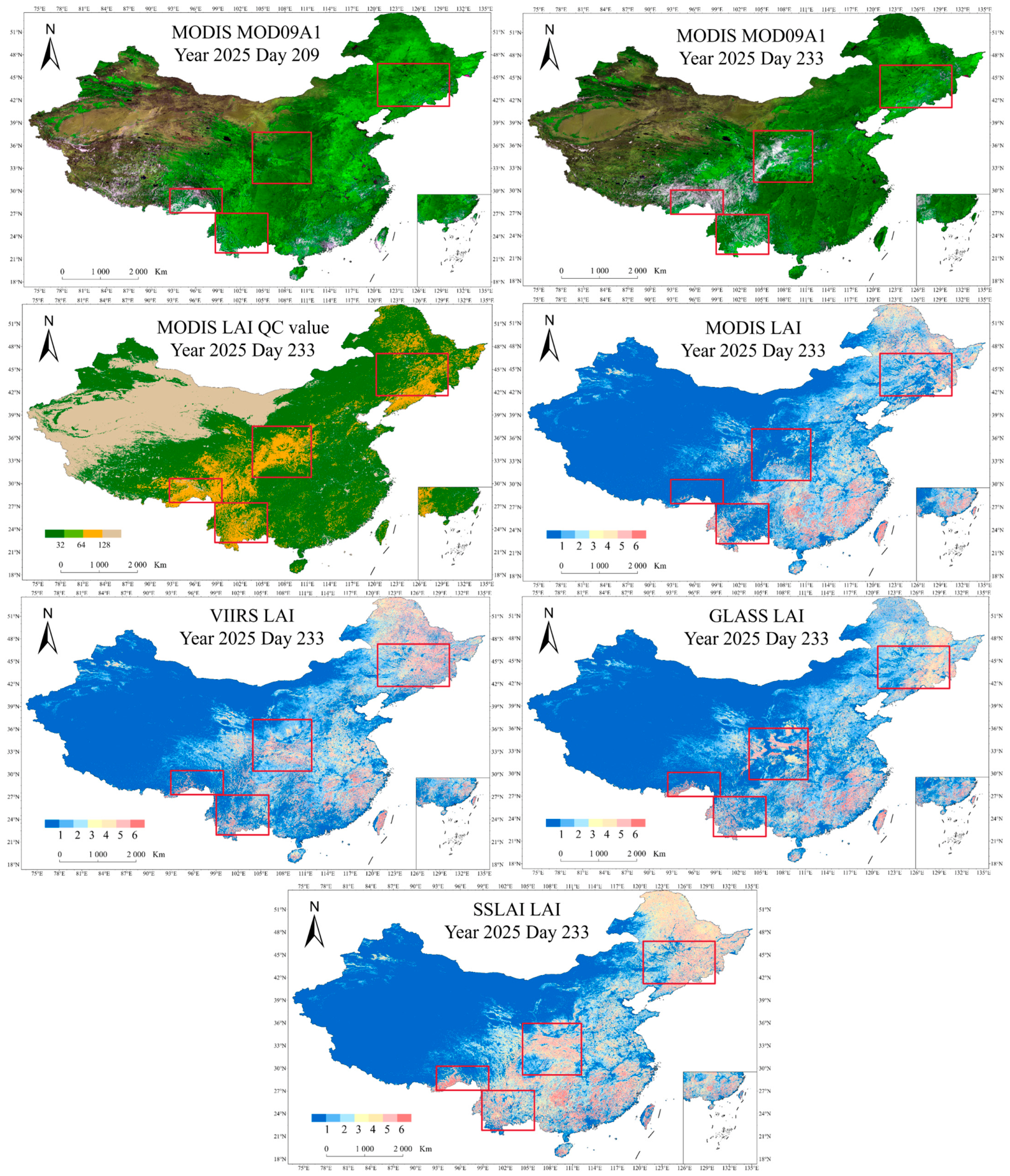
To assess the spatial consistency and reliability of the reconstructed LAI, Figure 9 displays the cloud-contaminated MODIS surface reflectance, the corresponding MODIS LAI QC map, and the spatial distributions of MODIS, VIIRS, GLASS, and the proposed SSLAI across China on Day 233, 2025. A temporally adjacent cloud-free MODIS surface reflectance image from Day 209, 2025, is also included as a reference. Day 233, 2025, was selected because it corresponds to the peak vegetation growing season with strong spatial heterogeneity across China. The four LAI products show similar general spatial patterns with higher values in southeastern China and lower values in northwestern China. Specifically, MODIS LAI exhibits greater uncertainty than SSLAI in high-latitude regions. In the Qinling Mountains, a major ecological boundary between northern and southern China, MODIS LAI presents severe data gaps, while GLASS and VIIRS LAI yield relatively low values. By contrast, only SSLAI maintains complete spatial continuity. In southern Yunnan and southern Xizang, MODIS and VIIRS LAI significantly underestimate LAI values in dense forests due to heavy cloud contamination in the contemporaneous MODIS surface reflectance on Day 233. GLASS LAI performs moderately better but still fails to represent the high LAI characteristics of tropical rainforests. Notably, SSLAI retains peak-season LAI magnitudes consistent with dense tropical and subtropical forests, as validated by the aforementioned cloud-free reference image. Furthermore, SSLAI substantially mitigates the influence of low-quality pixels identified in the MODIS LAI QC map. Therefore, SSLAI exhibits superior performance over other existing LAI products in spatial reconstruction during the peak growing season.

To further quantitatively validate these visual observations, comprehensive accuracy evaluations were conducted using 175 field LAI across five typical vegetation types in China (

Table 6. Quantitative comparison of MODIS, VIIRS, GLASS, and SSLAI against 175 field LAI (overall and by vegetation type). The best result in each category is marked in bold.

Category	Dataset	R2	RMSE	Bias
Overall	MODIS	0.728	0.612	−0.185
	VIIRS	0.756	0.574	−0.143
	GLASS	0.783	0.526	−0.107
	SSLAI	0.885	0.477	0.045
Forest	MODIS	0.715	0.632	−0.194
	VIIRS	0.742	0.591	−0.153
	GLASS	0.770	0.548	−0.118
	SSLAI	0.918	0.409	0.040
Grassland	MODIS	0.731	0.598	−0.179
	VIIRS	0.760	0.560	−0.138
	GLASS	0.788	0.519	−0.099
	SSLAI	0.860	0.518	0.053
Shrubland	MODIS	0.708	0.643	−0.206
	VIIRS	0.735	0.604	−0.168
	GLASS	0.762	0.557	−0.130
	SSLAI	0.872	0.485	0.048
Cropland	MODIS	0.726	0.625	−0.198
	VIIRS	0.753	0.587	−0.159
	GLASS	0.779	0.539	−0.121
	SSLAI	0.893	0.466	0.043
Desert	MODIS	0.682	0.789	−0.224
	VIIRS	0.710	0.735	−0.185
	GLASS	0.736	0.692	−0.147
	SSLAI	0.782	0.658	0.073

). Statistical metrics, including R², RMSE, and bias, were calculated for MODIS, VIIRS, GLASS, and SSLAI. Overall, SSLAI achieves the highest accuracy with an R² of 0.885, RMSE of 0.477, and bias of 0.045, outperforming all three existing LAI products. Spatially, SSLAI exhibits consistent superiority across forest, grassland, shrubland, cropland, and desert regions. In particular, SSLAI yields the best performance in dense forests with an R² of 0.918 and RMSE of 0.409, effectively reducing underestimation caused by cloud contamination. For croplands and grasslands, SSLAI also maintains higher consistency with ground observations, while all products show relatively lower accuracy in sparse desert vegetation. These quantitative results confirm that the proposed SSLAI provides more reliable, complete, and physically consistent LAI reconstructions than existing MODIS, VIIRS, and GLASS products, especially in cloudy regions and ecologically sensitive areas.

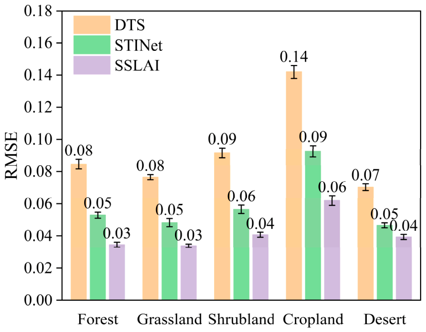
To quantify vegetation-specific accuracy, Figure 10 compares the RMSE of DTS, STINet, and SSLAI across five typical Chinese vegetation types: forest, grassland, shrubland, cropland, and desert. For a fair evaluation, DTS was selected as the baseline representing the best traditional method, and STINet was chosen as the baseline for the best deep learning method, as described in Section 4.1. The three models exhibit significant accuracy differences across vegetation types. DTS has the highest RMSE of 0.08 in forests. In grasslands, STINet’s RMSE is 0.02 higher than that of SSLAI at 0.05. In shrublands, DTS’s RMSE is 0.05 higher than that of SSLAI. In croplands, DTS’s RMSE is 0.05 higher than that of STINet and 0.08 higher than that of SSLAI. Notably, SSLAI achieves the lowest RMSE across all vegetation types, outperforming both DTS and STINet for each type and demonstrating strong cross-ecosystem generalization ability.

4.6. Sensitivity Analysis of Meteorological Covariates

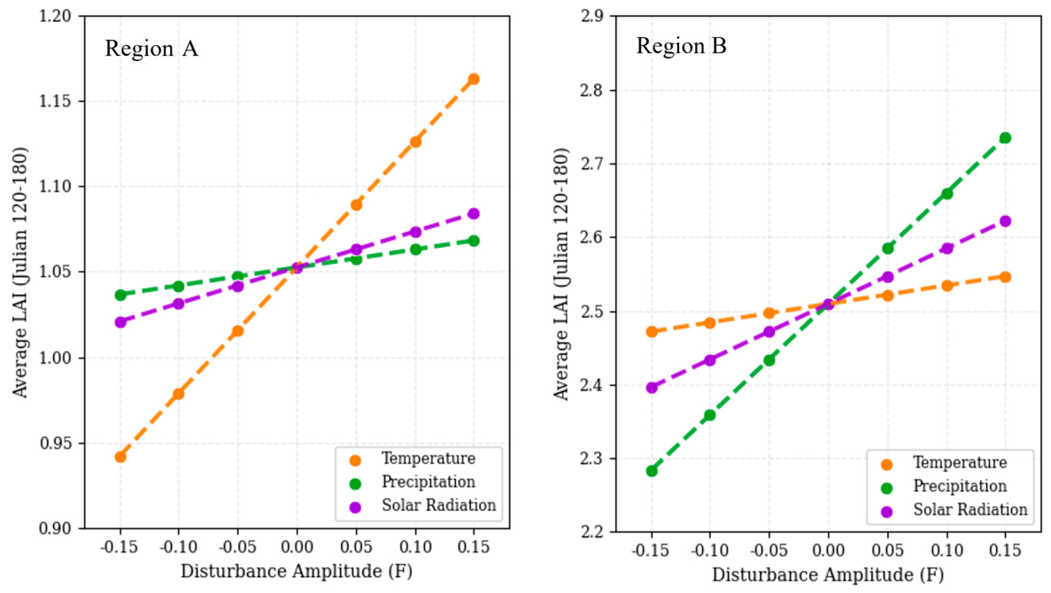
Sensitivity analysis of key meteorological drivers (CTP, CSSRD, and AT2) was conducted to quantify their regulatory roles in vegetation growth and to verify the physical reliability of the SSLAI reconstruction. The year 2018 was selected due to complete and high-quality MODIS LAI and meteorological records, providing a robust baseline for climatic perturbation experiments. Two typical ecosystems were chosen to reduce spatial heterogeneity: the alpine meadow core zone on the eastern Qinghai-Tibet Plateau (34.00–35.00° N, 96.00–97.00° E), characterized by a cold semi-humid climate; and the central North China Plain (36.00–37.00° N, 115.00–116.00° E), a region of intensive winter wheat cultivation. A scaling factor F ranging from −15% to +15% was applied to adjust individual meteorological variables while keeping other inputs unchanged, simulating realistic climate fluctuation scenarios. Model sensitivity was assessed using the mean LAI across valid pixels at ten sites during Julian days 120–180. Sensitivity results (Figure 11) reveal distinct regional climatic controls over vegetation growth. In Region A, AT2 exerted the strongest influence on regional average LAI, with LAI variations exceeding 0.2. In Region B, CTP dominated vegetation dynamics and produced the maximum LAI fluctuation of over 0.4. Such divergent response patterns further indicate that the SSLAI can effectively capture vegetation-specific feedback to local meteorological conditions across distinct geographical and environmental contexts.

4.7. Robustness Evaluation of LAI Time-Series Gap-Filling

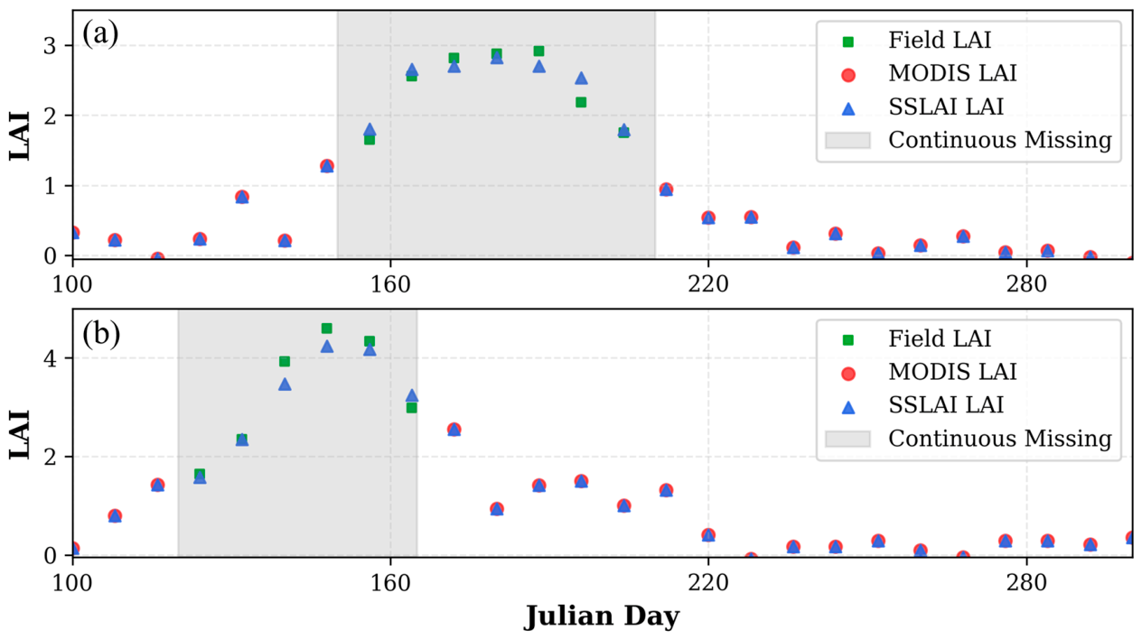
To evaluate the robustness of SSLAI in reconstructing LAI time series affected by cloud contamination, aerosol pollution, and sensor anomalies, two typical sites with long continuous missing periods were selected for visualization. The first site was an alpine meadow in the eastern Qinghai-Tibet Plateau (32.25° N, 97.50° E) that experienced a 60-day gap (JD150–210) in 2022. The second site was a winter wheat cropland in the North China Plain (37.87° N, 115.42° E) that suffered a 45-day gap (JD120–165) during the grain-filling stage in 2020. Figure 12 presents the gap-filling results of SSLAI. The original MODIS LAI time series contained long interruptions that disrupted natural vegetation growth trajectories, while SSLAI completely recovered the missing segments and produced smooth and ecologically consistent LAI variations. These results verify the robust gap-filling ability of SSLAI under severe long-term missing conditions.

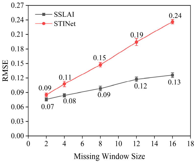
For quantitative robustness evaluation, an analysis of consecutive missing window sizes was performed with STINet as the baseline because it is the best-performing competing method. The experiment was carried out in the Xilingol Grassland (43.42–44.67° N, 115.50–117.17° E) using thirty random grassland pixels from 2019 to 2023. The study region and period were chosen for homogeneous vegetation, clear phenology, and stable interannual climate variability. Missing windows were set to 2, 4, 8, 12, and 16 MODIS 8-day composites, covering realistic gap scenarios from transient clouds to prolonged sensor anomalies. Figure 13 shows that RMSE values of both models increase with larger missing windows because of greater phenological information loss. However, SSLAI maintains significantly lower RMSE across all settings. Notably, SSLAI keeps RMSE below 0.20 even for the longest missing window. SSLAI maintains stable performance under varying window configurations, which is important for its practical application in large-scale LAI reconstruction for terrestrial ecosystem monitoring.

4.8. Sensitivity Analysis of Hyperparameters

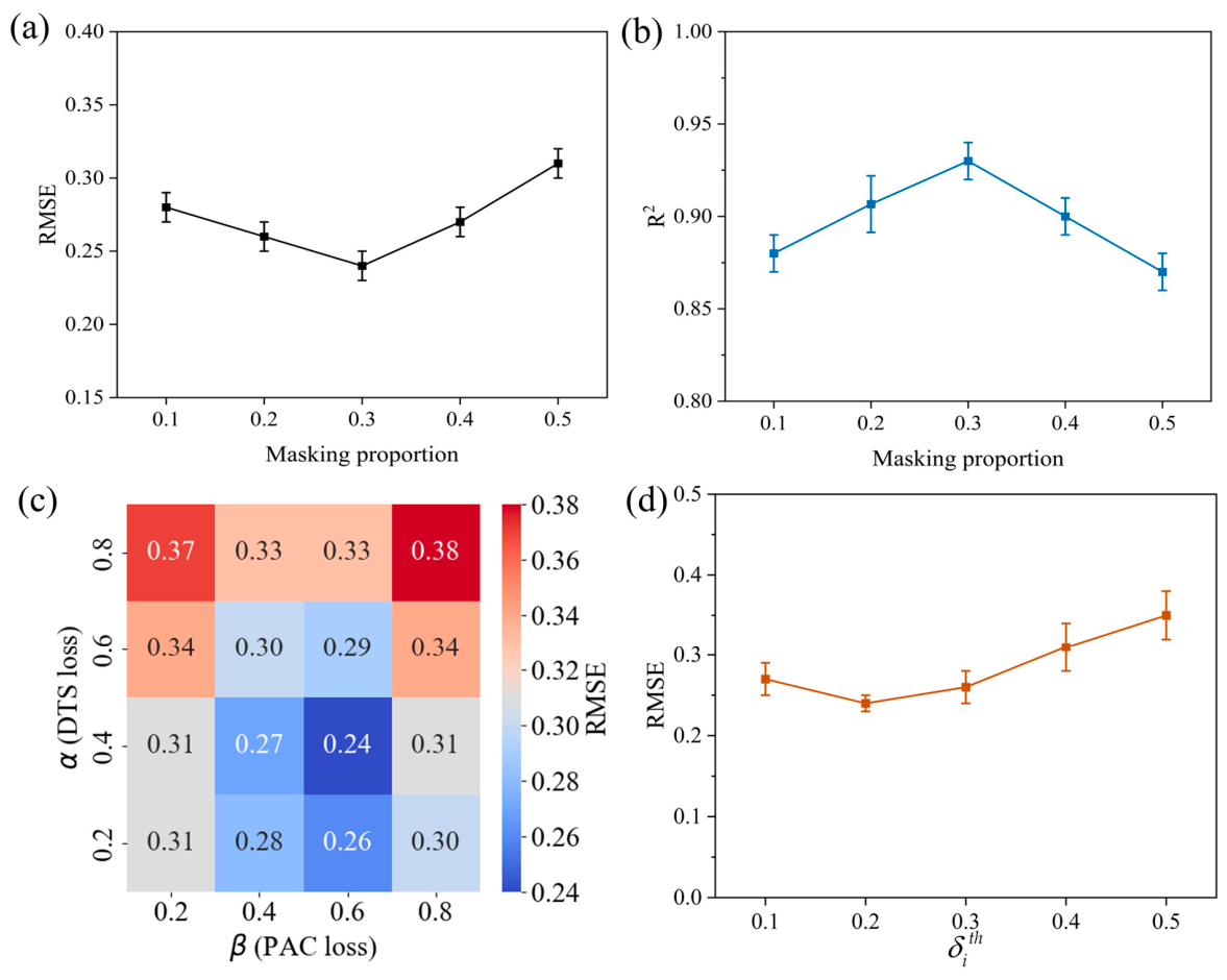
A systematic hyperparameter evaluation was conducted to verify the robustness and optimal parameter settings of SSLAI for ecological applications. Figure 14a,b show RMSE and R² changes under different self-supervised masking ratios. Insufficient masking provides limited samples for capturing temporal vegetation dependencies, leading to higher RMSE and lower R². The best performance is achieved at a moderate masking ratio (30%), which balances model learning and effective information retention. Excessively high ratios lead to information loss and unstable reconstruction, confirming that a moderate ratio is most suitable for capturing complex vegetation phenological patterns. Figure 14c presents the RMSE heatmap of the TAPC loss with different α and β coefficients. The lowest RMSE is obtained at the optimal combination (α = 0.4, β = 0.6), and any deviation degrades reconstruction accuracy. A low α value produces discontinuous LAI trends with limited smoothing, while an excessive α value suppresses real vegetation growth peaks. A low β value weakens ecological phenological constraints, whereas an overly high β value distorts natural vegetation growth rhythms. Figure 14d illustrates RMSE variations with the pixel-adaptive threshold in the DTS loss function. The RMSE follows a U-shaped distribution. A threshold of 0.2 achieves the best balance between noise reduction and genuine phenology preservation. An overly low threshold leaves residual noise, whereas an excessively high threshold removes useful phenological signals. This confirms that the optimal threshold ensures reliable temporal consistency and ecological rationality.

5. Discussion

5.1. Performance Advantages and Component Contribution Mechanism of the SSLAI Model

The experimental results demonstrate that SSLAI achieves the best performance in MODIS LAI reconstruction across China, mainly owing to the synergistic effect of its four core modules. According to the ablation analysis, the CPE module integrates MODIS LAI, meteorological drivers, and geospatial covariates to strengthen vegetation–environment coupling, which effectively improves the physical interpretability of LAI dynamics and increases the R² value to 0.83 compared with the baseline model. The MSTPP module enhances the representation of multi-scale temporal rhythms and spatial heterogeneity, reducing the RMSE by 13.51% and better capturing seasonal and interannual variations in vegetation growth. The STCA module models long-range dependencies in LAI time series, alleviating the limitation of local feature mining and decreasing the model bias by 33.33%. The TAPC loss function suppresses non-physiological fluctuations and unrealistic peaks, ensuring that reconstructed LAI aligns with natural vegetation growth rhythms. The combination of these modules yields the highest R² (0.93) and the lowest RMSE and bias, outperforming all comparison methods. Traditional gap-filling methods rely on fixed statistical functions and lack the ability to model nonlinear vegetation–climate relationships, resulting in low accuracy and failure to capture realistic phenological changes, especially under extreme climatic stress such as drought. Although Bi-LSTM and MBPNN capture partial temporal dependencies, they lack sufficient spatial modeling and generalization ability in heterogeneous landscapes, which is consistent with findings reported in previous remote sensing and LAI reconstruction studies [7,20]. State-of-the-art deep learning models, such as STINet and EDCSTFN, perform well in spatio-temporal feature extraction but still lack explicit ecological constraints on phenological patterns. In contrast, SSLAI stably reproduces seasonal cycles and climate-driven anomalies by integrating cross-modal environmental information and self-supervised learning, reducing dependence on labeled data while enhancing ecological consistency. This design differs fundamentally from traditional purely data-driven deep learning approaches that rely solely on data fitting without considering physical rationality or phenological regularity [53,54]. These advantages make SSLAI more suitable for large-scale vegetation dynamic monitoring and terrestrial ecosystem research.

5.2. Spatio-Temporal Reliability and Spatial Adaptability of the SSLAI Product in Complex Regions

Validation against field measurements confirms that SSLAI can reliably capture complex spatio-temporal variations in LAI, providing a high-quality data foundation for regional terrestrial vegetation monitoring. Compared with MODIS, VIIRS, and GLASS LAI products, SSLAI effectively reduces data gaps and underestimation in high-latitude regions caused by low solar angles and sensor noise [55]. In cloud-prone mountainous regions, such as the Qinling Mountains, southern Yunnan, and southern Xizang (Tibet), SSLAI maintains stronger spatial continuity and more reasonable vegetation gradient patterns than existing products. This finding is consistent with previous studies emphasizing the critical role of spatial continuity for LAI reconstruction in heterogeneous mountainous areas [56]. By reducing the influence of low-quality pixels flagged in the MODIS QC layer, SSLAI improves the overall reliability of LAI in ecologically sensitive areas. This finding is consistent with previous studies that have validated the importance of quality control and improved processing strategies for generating reliable long-term MODIS LAI products [51]. Across five major vegetation types in China (forest, grassland, shrubland, cropland, and desert), SSLAI achieves the lowest RMSE among all comparison methods, indicating stable performance under diverse vegetation and climatic conditions. Traditional methods, such as DTS, fail to capture fine phenological changes, while advanced deep learning methods lack sufficient phenological constraints. Our results are consistent with previous studies that have highlighted the necessity of incorporating phenological constraints and smoothing strategies to generate reliable and physically consistent LAI time series [11]. SSLAI therefore improves the spatio-temporal consistency and accuracy of LAI in heterogeneous landscapes, supporting key regional ecological applications including grassland degradation monitoring, cropland growth evaluation, and vegetation sensitivity analysis under climate change [57,58].

5.3. Sensitivity Analysis and Robustness Evaluation of the SSLAI Model

In the sensitivity analysis of meteorological covariates, AT2 variations dominated LAI dynamics in the alpine meadow ecosystem of the Qinghai-Tibet Plateau, while the effects of CTP and CSSRD were negligible. This finding confirms that temperature is the primary limiting factor for vegetation growth across the Qinghai-Tibet Plateau. By contrast, CTP exerted the strongest regulatory control on LAI in the farmland ecosystem of the North China Plain, followed by temperature and solar radiation, indicating that water availability acts as the key limiting factor for winter wheat growth. The climate sensitivity patterns identified in this study are also in line with previous findings, demonstrating that vegetation–climate relationships vary substantially across ecosystem types [7]. This analysis quantifies the linkage between meteorological conditions and vegetation growth, clarifies the physical mechanism underlying the reliable performance of SSLAI, and provides a theoretical basis for the reasonable selection of driving factors in large-scale terrestrial ecosystem monitoring. In the robustness evaluation, the SSLAI-filled LAI time series is in good agreement with in situ measurements, accurately capturing vegetation growth peaks and phenological rhythms without abnormal fluctuations. However, limited by its poor ability to capture inherent phenological characteristics, STINet exhibits a faster increase in RMSE with the expansion of data missing windows. This comparison further proves the superior robustness of the SSLAI framework. In addition, the hyperparameter evaluation outputs a stable and transferable parameter strategy, facilitating the scalable application of SSLAI across diverse terrestrial ecosystems. This scheme enables the widespread adoption of SSLAI in multiple fields, including forest inventory and carbon storage estimation [59], grassland monitoring and desertification assessment [60,61], crop growth and yield forecasting [62], and ecosystem service assessment and climate change impact analysis [63,64].

5.4. Limitations and Future Improvements

Despite the satisfactory results achieved in this study, several aspects require further improvement. First, the field sampling dataset has room for improvement. Increasing the number of sampling sites, optimizing spatial distribution, and supplementing multi-year continuous observations across typical and specialized study regions in future work will help reduce the uncertainty in LAI validation, especially under complex terrain conditions. Second, the vegetation classification in this study remains at a relatively general level. Adopting a more refined stratification scheme can further improve the interpretability of regional performance differences. Third, the computational complexity of the SSLAI framework is reasonable among existing deep learning methods. While such computational cost exerts no negative impact on reconstruction performance, subsequent network refinement is needed to further improve efficiency. Furthermore, the current SSLAI framework has only been validated using medium-resolution MODIS LAI products. Future studies will use higher-resolution remote sensing data to further examine its performance and generalization ability across different terrestrial ecosystems. Future research will focus on extending the SSLAI framework to high-resolution satellite datasets, collecting richer field measurement data, adopting more refined vegetation stratification schemes, and exploring lightweight network structures to balance accuracy and efficiency, thereby enabling more fine-scale vegetation dynamics monitoring and terrestrial ecological applications.

6. Conclusions

This study presents a self-supervised SSLAI framework for reconstructing MODIS LAI time series over large areas, aiming to mitigate spatio-temporal data gaps induced by cloud contamination and sensor noise. This framework provides key methodological advances for large-scale LAI reconstruction, with core functional modules designed to address critical limitations in time-series reconstruction. Specifically, the CPE module constructs a 3D spatio-temporal feature matrix and achieves heterogeneous feature fusion and dimensionality reduction via 3D CNN. An adaptive self-supervised masking strategy eliminates reliance on labeled data. A multi-scale spatio-temporal patch cross-attention mechanism enhances long-range temporal dependencies and spatial consistency. The TAPC loss function, which combines MAE, temporal smoothness constraints, and phenological consistency, effectively suppresses non-physiological fluctuations and preserves authentic vegetation phenological features. These innovations collectively enable accurate, physically interpretable, and scalable LAI reconstruction without ground-truth supervision.

Quantitative assessments and cross-comparison results fully validate the effectiveness and robustness of the proposed SSLAI framework. Comprehensive tests across China demonstrate that the proposed method outperforms seven conventional and advanced deep learning approaches. Even with 16 consecutive missing observation windows, SSLAI maintains strong reconstruction stability with an RMSE below 0.20. Field validation at 175 sites covering five vegetation types (2018–2025) yields an R² of 0.885 and an RMSE of 0.477. The reconstructed LAI responds consistently to meteorological drivers and conforms to ecological laws, indicating solid physical interpretability. In addition, SSLAI achieves superior spatial integrity and temporal continuity compared with MODIS, VIIRS, and GLASS products and performs reliably under changing climatic conditions.

Benefiting from the promising reconstruction performance demonstrated above, the high-quality gap-free LAI dataset generated by SSLAI provides a solid data basis for long-term vegetation dynamics monitoring, land surface modeling, and global change research. This study offers a practical and effective self-supervised solution for filling spatio-temporal gaps in remotely sensed vegetation parameters over large regions. It also provides a transferable paradigm for reconstructing other long-term satellite-derived biophysical products and supports in-depth investigations of terrestrial ecosystem responses to climate change.

References

1. Li, C.; Zhou, H.; Tang, J.; Wang, C.; Wang, Z.; Qi, J.; Yang, B.; Fang, R. Time-series high spatio-temporal resolution vegetation leaf area index estimation based on NDVI trends. Int. J. Appl. Earth Obs. Geoinf. 2025, 142, 104744. [Google Scholar] [CrossRef]
2. Wu, H.; Tian, T.; Geng, Q.; Li, H. STC-DeepLAINet: A transformer-GCN hybrid deep learning network for large-scale LAI inversion by integrating spatio-temporal correlations. Remote Sens. 2025, 17, 4047. [Google Scholar] [CrossRef]
3. Wang, X.; Zhang, Y.; Atkinson, P.M.; Zhang, K.R. Estimating spatiotemporally continuous GEDI aboveground biomass density during 2015–2020 from multisource data using machine learning and deep learning. IEEE J. Sel. Top. Appl. Earth Obs. Remote Sens. 2026, 19, 3839–3857. [Google Scholar] [CrossRef]
4. Fang, H.; Baret, F.; Plummer, S.; Schaepman-Strub, G. An overview of global leaf area index (LAI): Methods, products, validation, and applications. Rev. Geophys. 2019, 57, 739–799. [Google Scholar] [CrossRef]
5. Tang, K.; Chen, X.; Liu, T.; Li, A.; Tang, Y.; Yang, P.; Chen, J. AnytimeFormer: Fusing irregular and asynchronous SAR-optical time series to reconstruct reflectance at any given time. Remote Sens. Environ. 2026, 333, 115120. [Google Scholar] [CrossRef]
6. Yang, Y.; Li, P.; Feng, Z.; Rai, S.; Yang, H. Global landsat image acquisition probability: 1984–2023. Int. J. Appl. Earth Obs. Geoinf. 2025, 144, 104928. [Google Scholar] [CrossRef]
7. Zhu, X.; Li, J.; Liu, Q.; Yu, W.; Li, S.; Zhao, J.; Dong, Y.; Zhang, Z.; Zhang, H.; Lin, S. Use of a BP neural network and meteorological data for generating spatiotemporally continuous LAI time series. IEEE Trans. Geosci. Remote Sens. 2022, 60, 4405114. [Google Scholar] [CrossRef]
8. Liu, H.; Zhang, H.; Huang, B.; Yan, L.; Tran, K.K.; Qiu, Y.; Zhang, X.; Roy, D.P. Reconstruction of seamless harmonized Landsat Sentinel-2 (HLS) time series via self-supervised learning. Remote Sens. Environ. 2024, 308, 114191. [Google Scholar] [CrossRef]
9. Pu, J.; Yan, K.; Gao, S.; Zhang, Y.; Park, T.; Sun, X.; Weiss, M.; Knyazikhin, Y.; Myneni, R.B. Improving the MODIS LAI compositing using prior time-series information. Remote Sens. Environ. 2023, 287, 113493. [Google Scholar] [CrossRef]
10. Liu, T.; Jin, H.; Li, A.; Fang, H.; Wei, D.; Xie, X.; Nan, X. Estimation of vegetation leaf-area-index dynamics from multiple satellite products through deep-learning method. Remote Sens. 2022, 14, 4733. [Google Scholar] [CrossRef]
11. Huang, A.; Shen, R.; Di, W.; Han, H. A methodology to reconstruct LAI time series data based on generative adversarial network and improved Savitzky-Golay filter. Int. J. Appl. Earth Obs. Geoinf. 2021, 105, 102633. [Google Scholar] [CrossRef]
12. Wang, W.; Cao, R.; Liu, L.; Zhou, J.; Shen, M.; Zhu, X.; Chen, J. An Improved Spatiotemporal SavitzkyGolay (iSTSG) Method to Improve the Quality of Vegetation Index Time-Series Data on the Google Earth Engine. IEEE Trans. Geosci. Remote Sens. 2025, 63, 4401917. [Google Scholar] [CrossRef]
13. Suseno, B.; Brunel, G.; Wijayanto, H.; Sadik, K.; Afendi, F.M.; Tisseyre, B. Reconstructing satellite temporal series data under cloudy conditions: Application in predicting rice growth phases. Smart Agric. Technol. 2025, 12, 101378. [Google Scholar] [CrossRef]
14. Wang, C.; Zhang, G.; Xie, J.; Yang, Y.; Chen, R.; Wang, M.; Xu, B.; Yin, G. Reconstructing red-edge vegetation indices from landsat 8 to improve leaf area index estimation. IEEE J. Sel. Top. Appl. Earth Obs. Remote Sens. 2025, 18, 24479–24490. [Google Scholar] [CrossRef]
15. Qian, S.; Xue, Z.; Jia, M.; Zhang, H. Streamlined multilayer perceptron for contaminated time series reconstruction: A case study in coastal zones of southern China. ISPRS J. Photogramm. Remote Sens. 2025, 221, 193–209. [Google Scholar] [CrossRef]
16. Perach, O.; Solomon, N.; Avneri, A.; Ram, O.; Abbo, S.; Herrmann, I. Integrating Sentinel-2 imagery and meteorological data to estimate leaf area index and leaf water potential, with a leave-field-out validation strategy in chickpea fields. Eur. J. Agron. 2025, 168, 127632. [Google Scholar] [CrossRef]
17. Tao, J.; Wang, Y.; Qiu, B.; Wu, W. Exploring cropping intensity dynamics by integrating crop phenology information using Bayesian networks. Comput. Electron. Agric. 2022, 193, 106667. [Google Scholar] [CrossRef]
18. Zhang, H.; Luo, Y.; Zhang, L.; Wu, Y.; Wang, M.; Shen, Z. Considering three elements of aesthetics: Multi-task self-supervised feature learning for image style classification. Neurocomputing 2023, 520, 262–273. [Google Scholar] [CrossRef]
19. Zhou, Y.; Wang, S.; Wu, T.; Feng, L.; Wu, W.; Luo, J.; Zhang, X.; Yan, N. For-backward LSTM-based missing data reconstruction for time-series Landsat images. GISci. Remote Sens. 2022, 59, 410–430. [Google Scholar] [CrossRef]
20. Chen, B.; Zheng, H.; Wang, L.; Hellwich, O.; Chen, C.; Yang, L.; Liu, T.; Luo, G.; Bao, A.; Chen, X. A joint learning Im-BiLSTM model for incomplete time-series Sentinel-2A data imputation and crop classification. Int. J. Appl. Earth Obs. Geoinf. 2022, 108, 102762. [Google Scholar] [CrossRef]
21. Stucker, C.; Garnot, V.S.; Schindler, K. U-TILISE: A sequence-to-sequence model for cloud removal in optical satellite time series. IEEE Trans. Geosci. Remote Sens. 2023, 61, 5408716. [Google Scholar] [CrossRef]
22. Chen, P.; Zhou, K.; Fang, H. High-resolution seamless mapping of the leaf area index via multisource data and the transformer deep learning model. IEEE Trans. Geosci. Remote Sens. 2025, 63, 4408512. [Google Scholar] [CrossRef]
23. Xu, Y.; Ma, Y.; Zhang, Z. Self-supervised pre-training for large-scale crop mapping using sentinel-2 time series. ISPRS J. Photogramm. Remote Sens. 2024, 207, 312–325. [Google Scholar] [CrossRef]
24. Devlin, J.; Chang, M.; Lee, K.; Toutanova, K. BERT: Pre-training of deep bidirectional transformers for language understanding. In Proceedings of the 2019 Conference of the North American Chapter of the Association for Computational Linguistics: Human Language Technologies, Minneapolis, MN, USA, 2–7 June 2019. [Google Scholar] [CrossRef]
25. Dumeur, I.; Valero, S.; Inglada, J. Self-supervised spatio-temporal representation learning of satellite image time series. IEEE J. Sel. Top. Appl. Earth Obs. Remote Sens. 2024, 17, 4350–4367. [Google Scholar] [CrossRef]
26. Yuan, Y.; Lin, L. Self-supervised pretraining of transformers for satellite image time series classification. IEEE J. Sel. Top. Appl. Earth Obs. Remote Sens. 2021, 14, 474–487. [Google Scholar] [CrossRef]
27. Zhao, L.; Zhang, X.; Wang, Z. Focusing on neglected natural images: A self-supervised learning model for pan-sharpening. Inf. Process. Manag. 2025, 62, 104246. [Google Scholar] [CrossRef]
28. Brinkhoff, J.; Houborg, R.; Clark, A. Empirical correction of sentinel-2 time series data to enhance real-time rice crop monitoring. IEEE J. Sel. Top. Appl. Earth Obs. Remote Sens. 2025, 18, 25391–25409. [Google Scholar] [CrossRef]
29. Bouchat, J.; Deffense, Q.; De Maet, T.; Defourny, P. Synergistic use of optical and SAR imagery for near real-time green area index retrieval in maize. IEEE J. Sel. Top. Appl. Earth Obs. Remote Sens. 2025, 18, 28515–28530. [Google Scholar] [CrossRef]
30. Friedl, M.; Sulla-Menashe, D. MODIS/Terra+Aqua Land Cover Type Yearly L3 Global 500m SIN Grid V061. NASA Land Processes Distributed Active Archive Center. 2022. Available online: https://www.earthdata.nasa.gov/data/catalog/lpcloud-mcd12q1-061 (accessed on 31 January 2026).
31. Myneni, R.B.; Hoffman, S.; Knyazikhin, Y.; Privette, J.L.; Glassy, J.; Tian, Y.; Wang, Y.; Song, X.; Zhang, Y.; Smith, G.R.; et al. Global products of vegetation leaf area and fraction absorbed PAR from year one of MODIS data. Remote Sens. Environ. 2002, 83, 214–231. [Google Scholar] [CrossRef]
32. Muñoz Sabater, J. ERA5-Land Hourly Data from 1950 to Present. Copernicus Climate Change Service (C3S) Climate Data Store (CDS). 2019. Available online: https://cds.climate.copernicus.eu/datasets/reanalysis-era5-land?tab=overview (accessed on 15 February 2026).
33. Reuter, H.I.; Nelson, A.; Jarvis, A. An evaluation of void-filling interpolation methods for SRTM data. Int. J. Geogr. Inf. Sci. 2007, 21, 983–1008. [Google Scholar] [CrossRef]
34. Didan, K. MODIS/Terra Vegetation Indices 16-Day L3 Global 500m SIN Grid V061 [Data Set]. 2021. NASA Land Processes Distributed Active Archive Center. Available online: https://www.earthdata.nasa.gov/data/catalog/lpcloud-mod13a1-061 (accessed on 2 March 2026).
35. Wang, S.; Fan, F. STINet: Vegetation changes reconstruction through a transformer-based spatiotemporal fusion approach in remote sensing. IEEE Trans. Geosci. Remote Sens. 2024, 62, 4412116. [Google Scholar] [CrossRef]
36. Yuan, H.; Dai, Y.; Xiao, Z.; Ji, D.; Shangguan, W. Reprocessing the MODIS leaf area index products for land surface and climate modelling. Remote Sens. Environ. 2011, 115, 1171–1187. [Google Scholar] [CrossRef]
37. Ma, Y.; Wang, W.; Jin, S.; Li, H.; Liu, B.; Gong, W.; Fan, R.; Li, H. Spatiotemporal variation of LAI in different vegetation types and its response to climate change in China from 2001 to 2020. Ecol. Indic. 2023, 156, 111101. [Google Scholar] [CrossRef]
38. Ji, S.; Xu, W.; Yang, M.; Yu, K. 3D Convolutional Neural Networks for Human Action Recognition. IEEE Trans. Pattern Anal. Mach. Intell. 2013, 35, 221–232. [Google Scholar] [CrossRef] [PubMed]
39. Rogers, C.; Chen, J.; Croft, H.; Gonsamo, A.; Luo, X.; Bartlett, P.; Staebler, R. Daily leaf area index from photosynthetically active radiation for long term records of canopy structure and leaf phenology. Agric. For. Meteorol. 2021, 304, 108407. [Google Scholar] [CrossRef]
40. Wengert, M.; Piepho, H.; Astor, T.; Grass, R.; Wachendorf, M.; Wijesingha, J. Spatial-temporal heterogeneity of yield, protein concentration, and leaf area index in grassland agroforestry systems can be modeled from UAV-borne imagery. Comput. Electron. Agric. 2025, 237, 110575. [Google Scholar] [CrossRef]
41. Wang, J.; Xie, H.; Wang, F.; Lee, L. A transformer-convolution model for enhanced session-based recommendation. Neurocomputing 2023, 531, 21–33. [Google Scholar] [CrossRef]
42. Liao, D.; Shi, C.; Wang, L. A spectral-spatial fusion transformer network for hyperspectral image classification. IEEE Trans. Geosci. Remote Sens. 2023, 61, 5515216. [Google Scholar] [CrossRef]
43. Wu, H.; Xu, J.; Wang, J.; Long, M. Autoformer: Decomposition transformers with auto-correlation for long-term series forecasting. In Proceedings of the 35th Conference on Neural Information Processing Systems, Online, 6–14 December 2021. [Google Scholar]
44. Jiang, H.; Li, D.; Zhao, J.; Mu, Z.; Wu, F. GAPatch: Graph-aware patch-based transformers for long-horizon time series forecasting. Knowl.-Based Syst. 2026, 336, 115246. [Google Scholar] [CrossRef]
45. Nie, Y.; Nguyen, N.H.; Sinthong, P.; Kalagnanam, J. A Time Series is Worth 64 Words: Long-term Forecasting with Transformers. In Proceedings of the International Conference on Learning Representations (ICLR), 2023, Kigali, Rwanda, 1–5 May 2023. [Google Scholar]
46. Ge, J.; Zhang, H.; Zuo, L.; Xu, L.; Jiang, J.; Song, M.; Ding, Y.; Xie, Y.; Wu, F.; Wang, C.; et al. Large-scale rice mapping under spatiotemporal heterogeneity using multi-temporal SAR images and explainable deep learning. ISPRS J. Photogramm. Remote Sens. 2025, 220, 395–412. [Google Scholar] [CrossRef]
47. Wang, H.; Gao, X.; Jiang, W.; Lang, X.; Hu, X.; Qiu, M.; Guo, Q.; Liang, Y.; Wang, X.; Mu, Y.; et al. PMTFIM: Integrating machine learning with nutrient balance theory to estimate multi-stage paddy fertilization information at field scale over large regions. ISPRS J. Photogramm. Remote Sens. 2025, 230, 693–715. [Google Scholar] [CrossRef]
48. Ji, J.; Li, X.; Du, H.; Mao, F.; Fan, W.; Xu, Y.; Huang, Z.; Wang, J.; Kang, F. Multiscale leaf area index assimilation for Moso bamboo forest based on Sentinel-2 and MODIS data. Int. J. Appl. Earth Obs. Geoinf. 2021, 104, 102519. [Google Scholar] [CrossRef]
49. Graesser, J.; Stanimirova, R.; Friedl, M.A. Reconstruction of satellite time series with a dynamic smoother. IEEE J. Sel. Top. Appl. Earth Obs. Remote Sens. 2022, 15, 1803–1813. [Google Scholar] [CrossRef]
50. Li, M.; Wang, P.; Tansey, K.; Guo, F.; Zhou, J. Improved leaf area index reconstruction in heavily cloudy areas: A novel deep learning approach for SAR-Optical fusion integrating spatiotemporal features. Int. J. Appl. Earth Obs. Geoinf. 2025, 142, 104745. [Google Scholar] [CrossRef]
51. Lin, W.; Yuan, H.; Dong, W.; Zhang, S.; Liu, S.; Wei, N.; Lu, X.; Wei, Z.; Hu, Y.; Dai, Y. Reprocessed MODIS Version 6.1 Leaf Area Index Dataset and Its Evaluation for Land Surface and Climate Modeling. Remote Sens. 2023, 15, 1780. [Google Scholar] [CrossRef]
52. Liu, D.; Silveira, E.M.O.; Razenkova, E.; Anand, A.; Dubinin, M.; Hobi, M.; Pidgeon, A.M.; Radeloff, V.C. Global dynamic habitat indices (DHIs) based on MODIS and VIIRS vegetation products. Remote Sens. Environ. 2026, 332, 115099. [Google Scholar] [CrossRef]
53. Ma, H.; Liang, S. Development of the GLASS 250-m leaf area index product (version 6) from MODIS data using the bidirectional LSTM deep learning model. Remote Sens. Environ. 2022, 273, 112985. [Google Scholar] [CrossRef]
54. Liu, T.; Jin, H.; Xie, X.; Fang, H.; Wei, D.; Li, A. Bi-LSTM model for time series leaf area index estimation using multiple satellite products. IEEE Geosci. Remote Sens. Lett. 2022, 19, 2506805. [Google Scholar] [CrossRef]
55. Peng, T.; Wang, M.; Wu, Q.; Chen, R.; Pan, J.; Lan, Q. A color correction method for multiple nonuniformly illuminated Whisk-Broom optical satellite images. IEEE Trans. Geosci. Remote Sens. 2025, 63, 5655420. [Google Scholar] [CrossRef]
56. Zhang, G.; Ni, Y.; Sun, G.; Liu, X.; Zhang, Y.; Hu, J.; Li, Z.; Chen, R.; Wang, M.; Yin, G.; et al. Real-time generation of gap-free MODIS leaf area index product from 2000 to 2024 using a deep learning method. Int. J. Appl. Earth Obs. Geoinf. 2026, 148, 105240. [Google Scholar] [CrossRef]
57. Zhang, Y.; Wang, P.; Tansey, K.; Han, D.; Chen, C.; Liu, J.; Li, H. Enhanced feature extraction from assimilated VTCI and LAI with a particle filter for wheat yield estimation using Cross-Wavelet transform. IEEE J. Sel. Top. Appl. Earth Obs. Remote Sens. 2023, 16, 5115–5127. [Google Scholar] [CrossRef]
58. Han, D.; Wang, P.; Tansey, K.; Liu, J.; Zhang, Y.; Tian, H.; Zhang, S. Integrating an attention-based deep learning framework and the SAFY-V model for winter wheat yield estimation using time series SAR and optical data. Comput. Electron. Agric. 2022, 201, 107334. [Google Scholar] [CrossRef]
59. Sinan, M.; Hasenauer, H. How to determine the leaf area index (LAI) of forests: A comparison of forest inventory versus satellite-driven estimates. For. Ecosyst. 2025, 13, 100332. [Google Scholar] [CrossRef]
60. Hu, Z.; Piao, S.; Knapp, A.; Wang, X.; Peng, S.; Yuan, W.; Running, S.; Mao, J.; Shi, X.; Ciais, P.; et al. Decoupling of greenness and gross primary productivity as aridity decreases. Remote Sens. Environ. 2022, 279, 113120. [Google Scholar] [CrossRef]
61. Li, N.; Wang, D. Quantifying time-lag and time-sccumulation effects of climate change and human activities on vegetation dynamics in the Yarlung Zangbo river basin of the Tibetan Plateau. Remote Sens. 2025, 17, 160. [Google Scholar] [CrossRef]
62. Yokoyama, Y.; de Wit, A.; Matsui, T.; Tanaka, T.S.T. Accuracy and robustness of a plant-level cabbage yield prediction system generated by assimilating UAV-based remote sensing data into a crop simulation model. Precis. Agric. 2024, 25, 2685–2702. [Google Scholar] [CrossRef]
63. Wu, D.; Bao, S.; Tong, Y.; Fan, Y.; Lu, L.; Liu, S.; Li, W.; Xue, M.; Cao, B.; Li, Q.; et al. Leaf area index estimation of grassland based on UAV-Borne hyperspectral data and multiple machine learning models in Hulun Lake Basin. Remote Sens. 2025, 17, 2914. [Google Scholar] [CrossRef]
64. Singh, A.; Göhner, C.S.; Stendardi, L.; Claus, M.; Cuozzo, G.; Jacob, A.; Castelli, M. A Transformer-based convolutional regressor to include SAR backscatter signals in monitoring alpine grasslands. IEEE Geosci. Remote Sens. Lett. 2026, 23, 2501205. [Google Scholar] [CrossRef]
Figure 1. Spatial distribution of vegetation types in China.
Land 15 00833 g001
Figure 2. Distribution proportion of different vegetation types in the training dataset.
Land 15 00833 g002
Figure 3. Workflow of the proposed SSLAI framework for MODIS LAI spatio-temporal reconstruction. (a) Multi-scale Spatio-temporal Patch Perception Module; (b) Spatio-temporal Cross-attention Module.
Land 15 00833 g003
Figure 4. MODIS LAI adaptive self-supervised masking strategy.
Land 15 00833 g004
Figure 5. Performance comparison of eight methods for 500 m MODIS LAI reconstruction across China in terms of R2, RMSE, and bias. (a) R2; (b) RMSE; (c) Bias.
Land 15 00833 g005
Figure 6. Comparison of LAI time series reconstructed by eight competing models and the field LAI across three representative biomes. (a) Winter wheat–summer maize rotation system in Langfang, Hebei Province (2019); (b) alpine meadow in Diqing Tibetan Autonomous Prefecture, Yunnan Province (2018); (c) deciduous coniferous forest in the northern Greater Khingan Mountains (2020).
Land 15 00833 g006
Figure 7. Scatter plot of SSLAI-reconstructed LAI versus field LAI (2018–2022).
Land 15 00833 g007
Figure 8. Long-term time-series comparison of LAI products (MODIS, GLASS, and SSLAI) for a representative site in the Xilingol Grassland, Inner Mongolia, China, during 2015–2025.
Land 15 00833 g008
Figure 9. Spatial distributions of MODIS surface reflectance imagery (Year 2025 Day 209 and Day 233), the MODIS LAI QC layer, and four LAI products (MODIS, VIIRS, GLASS, and the proposed SSLAI) on Year 2025 Day 233 across China.
Land 15 00833 g009
Figure 10. RMSE comparison of DTS, STINet, and SSLAI over five typical vegetation types in China (forest, grassland, shrubland, cropland, and desert).
Land 15 00833 g010
Figure 11. Relationship between the reconstructed LAI and F for each meteorological factor on Julian days 120–180.
Land 15 00833 g011
Figure 12. Visualization of LAI time-series gap-filling results by the SSLAI under long-duration missing data scenarios. (a) Alpine meadow in the eastern Qinghai-Tibet Plateau in 2022; (b) winter wheat cropland in the North China Plain in 2020.
Land 15 00833 g012
Figure 13. RMSE variations of SSLAI and STINet under different consecutive missing window sizes.
Land 15 00833 g013
Figure 14. Hyperparameter sensitivity analysis of the proposed SSLAI. (a) RMSE as a function of self-supervised masking ratio (0.1–0.5); (b) R2 as a function of self-supervised masking ratio (0.1–0.5); (c) RMSE heatmap for different combinations of α (DTS loss coefficient) and β (PAC loss coefficient); (d) RMSE sensitivity to the pixel-adaptive threshold of the first-order difference slope (0.1–0.5).
Land 15 00833 g014