Operational and Temporal Correlates of Wildfire Size: A 10-Year Analysis from Central Anatolia, Türkiye

Abstract

Background: Administrative wildfire records can characterize operational and temporal patterns, but causal interpretation requires caution when meteorological, fuel, topographic, and accessibility variables are unavailable. This study examined factors associated with wildfire size within the jurisdiction of the Kayseri Regional Directorate of Forestry, Türkiye, during 2016–2025. Methods: A total of 364 wildfire records were analyzed. Large-fire risk (>5 ha) was modeled with Firth-penalized logistic regression because of sparse events and separation. Burned area was analyzed using a two-part model: Firth logistic regression for zero versus positive burned area, followed by a Gamma generalized linear model with a log link for positive burned area (n = 333). Seasons were treated as categorical variables using calendar definitions, and the administrative vehicle-count variable was reported descriptively because its timing could not be verified as initial dispatch. Mann–Kendall trend tests, corrected seasonal post hoc comparisons, and exploratory ROC analysis were also performed. Results: Fifty-six fires (15.4%) exceeded 5 ha, and 31 records had zero burned area. Negligence/carelessness was the recorded cause in 91.5% of incidents. In the Firth large-fire model, initial response time was not independently associated with large-fire odds (OR = 1.007, 95% CI 0.989–1.026; p = 0.452), and no modeled predictor reached statistical significance. In the positive-area Gamma component, autumn fires had greater conditional mean burned area than summer fires (mean ratio [MR] = 1.683, 95% CI 1.233–2.295; p = 0.001), whereas initial response time was not statistically significant (MR = 1.012, 95% CI 0.998–1.026; p = 0.097). Seasonal distributions differed overall (Kruskal–Wallis H = 12.759, p = 0.005; epsilon-squared = 0.027), with the Holm-corrected autumn-versus-summer comparison remaining significant (p = 0.035). Response time alone showed weak discrimination for large fires (AUC = 0.562, bootstrap 95% CI 0.489–0.636); the 18 min value was therefore retained only as a dataset-specific exploratory reference. The response-time trend was not statistically significant (tau = −0.467, p = 0.073), and excluding 2025 further attenuated it (tau = −0.333, p = 0.260). Conclusions: The corrected analyses support seasonal heterogeneity, particularly greater positive burned area in autumn, but do not support a causal or independently significant response-time effect after conservative model specification. Future wildfire-response analyses should integrate weather, fuels, terrain, access, distance, and incident conditions at detection.

1. Introduction

Wildfire outcomes emerge from interactions among weather, fuels, topography, ignition processes, land use, and suppression systems [1,2,3,4,5]. In inhabited and fragmented forest landscapes, operational response is therefore relevant to risk management, but it represents only one component of wider socio-ecological resilience. Resilience and territorial planning frameworks emphasize the need to integrate ecosystem information, settlement patterns, and spatial planning rather than infer governance performance from operational records alone [6,7].

Temporal concentration is a defining feature of wildfire regimes. Temperature, drought, atmospheric dryness, and seasonal fuel conditions can extend fire seasons and alter the timing of high-risk periods [8,9,10]. Mediterranean studies also show that ignition timing and final fire size may differ by cause and season [11,12]. For regional administrative datasets, calendar month, season, and time of day can therefore provide useful descriptive and associative information, although they cannot substitute for direct meteorological measurements.

Initial response time is a commonly used operational indicator because delays may reflect travel distance, access constraints, resource positioning, concurrent incidents, or dispatch processes [13,14,15,16]. Evidence from initial-attack studies indicates that containment probability depends jointly on response time, terrain, fire behavior, fuel conditions, weather, and accessibility [14,17,18,19]. Consequently, response time should be interpreted as an operational correlate and possible proxy for unmeasured access conditions rather than as an isolated causal determinant of final fire size.

Burned area is highly right-skewed in most wildfire datasets, with many small events and relatively few large incidents [20,21,22,23,24]. This distribution creates two related analytic questions: whether a fire produces measurable burned area and, conditional on positive area, how large the final burned area becomes. Likewise, defining a large fire by a fixed threshold can be operationally useful but discards information contained in the continuous distribution. A combined binary and continuous modeling strategy can therefore provide a more complete assessment.

Spatial context is also important. Fire susceptibility, initial-attack success, and exposure can vary across administrative units because of differences in access, settlement patterns, terrain, vegetation, and infrastructure [14,25,26,27]. Recent WUI research demonstrates that the configuration of vegetation and built structures influences exposure and that fine-scale mapping can support locally tailored mitigation [7]. The present administrative dataset does not contain incident coordinates or WUI indicators; these concepts are therefore used only to contextualize future spatial extensions of the analysis.

The Kayseri Regional Directorate of Forestry in Türkiye (KRDF) provides a useful regional case because its jurisdiction spans semi-arid Central Anatolian landscapes, forest–agriculture interfaces, and multiple forestry directorates. Official records over ten years allow examination of temporal patterns, recorded ignition causes, operational timing, administrative location, and burned area within one management system.

The source workbook also contains a category labeled “type”; inspection of the coding key showed that this variable represents dominant vegetation or land-cover categories (for example, oak, Scots pine, black pine, degraded land, and agricultural land), not a fire-behavior or fire-type classification. Accordingly, it was not interpreted as a wildfire type variable, and claims based on fire-behavior typologies were removed from the analytic framework.

This study therefore focuses on operational and temporal correlates of wildfire size rather than on direct measurement of governance or forest-city resilience. The aims were to (1) describe temporal, causal, spatial, and operational characteristics of wildfire records; (2) estimate associations with large-fire occurrence and burned area using methods robust to separation and zero outcomes; and (3) identify data limitations that should be addressed in future integrated wildfire-risk analyses.

Three a priori hypotheses were evaluated: H1, longer initial response time would be associated with greater burned area and higher odds of a large fire; H2, burned-area distributions would differ across calendar seasons; and H3, recorded ignition cause, time of day, and forestry directorate would show associations with fire outcomes after adjustment. Vehicle count was not included in these hypotheses because the source label identifies “vehicles used” and does not establish that the value was known at initial dispatch.

2. Materials and Methods

This section describes the data source, data-quality checks, variable definitions, and analytical procedures used for wildfire records within KRDF during 2016–2025.

2.1. Study Area

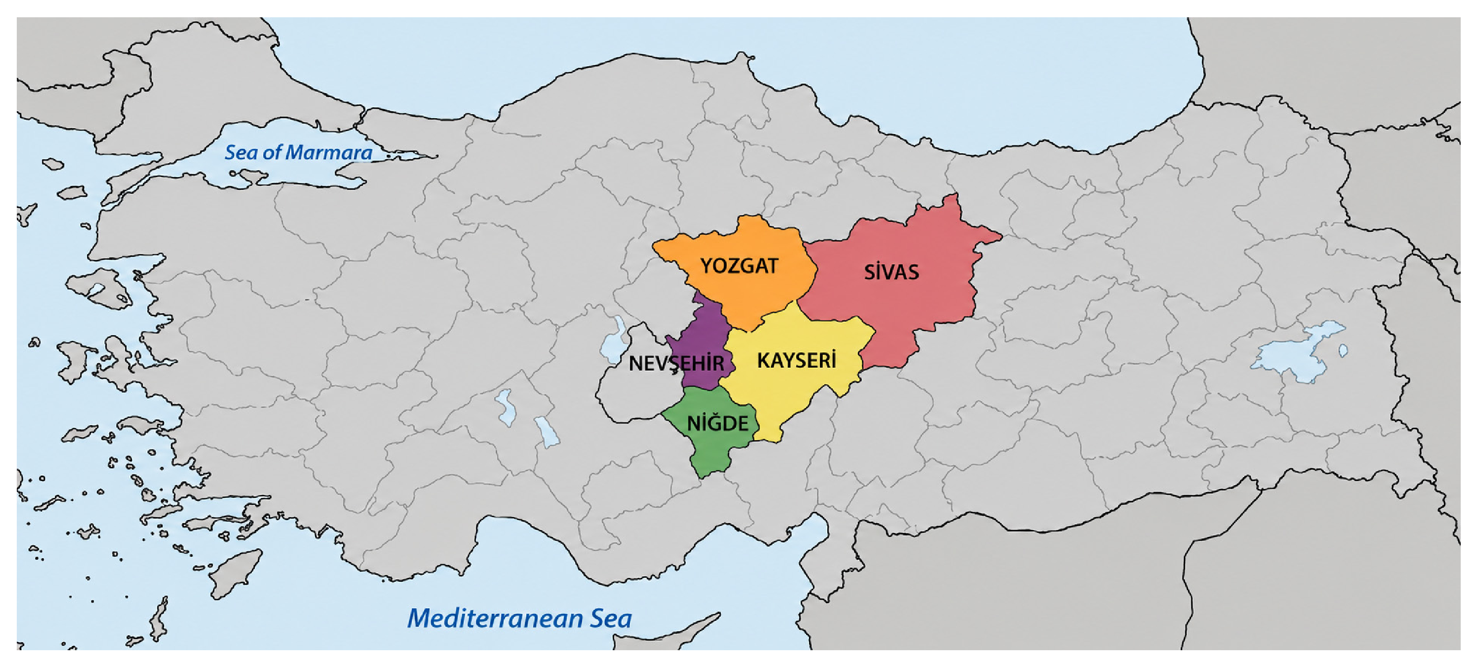
KRDF covers a broad part of Central Anatolia, including areas within Kayseri, Sivas, Yozgat, Nigde, and Nevsehir. The jurisdiction spans semi-arid continental landscapes, plateaus, agricultural–forest mosaics, and mountainous terrain, including the Erciyes massif and higher-elevation forest areas [28,29]. These characteristics are relevant to wildfire analysis because terrain, road access, and the continuity of forest and agricultural fuels can vary substantially across the region.

Forests within the responsibility area include deciduous, coniferous, and degraded stands, with oak, black pine, and trembling aspen among the reported species [29]. The source data do not provide incident-level fuel continuity, slope, aspect, road distance, or station distance; these environmental and accessibility factors were therefore not modeled directly.

Previous regional descriptions indicate that wildfire occurrence is concentrated mainly in summer and early autumn, particularly around July–September [30,31]. In the present study, seasons were defined strictly by calendar month: spring = March–May, summer = June–August, autumn = September–November, and winter = December–February. This definition is used consistently in all analyses and tables.

The region includes forest–agriculture interfaces, pasture transitions, and areas near settlements where human activity may contribute to ignition risk [32,33]. These features make KRDF suitable for a regional operational analysis, while the absence of incident coordinates prevents direct WUI or accessibility mapping in the current dataset.

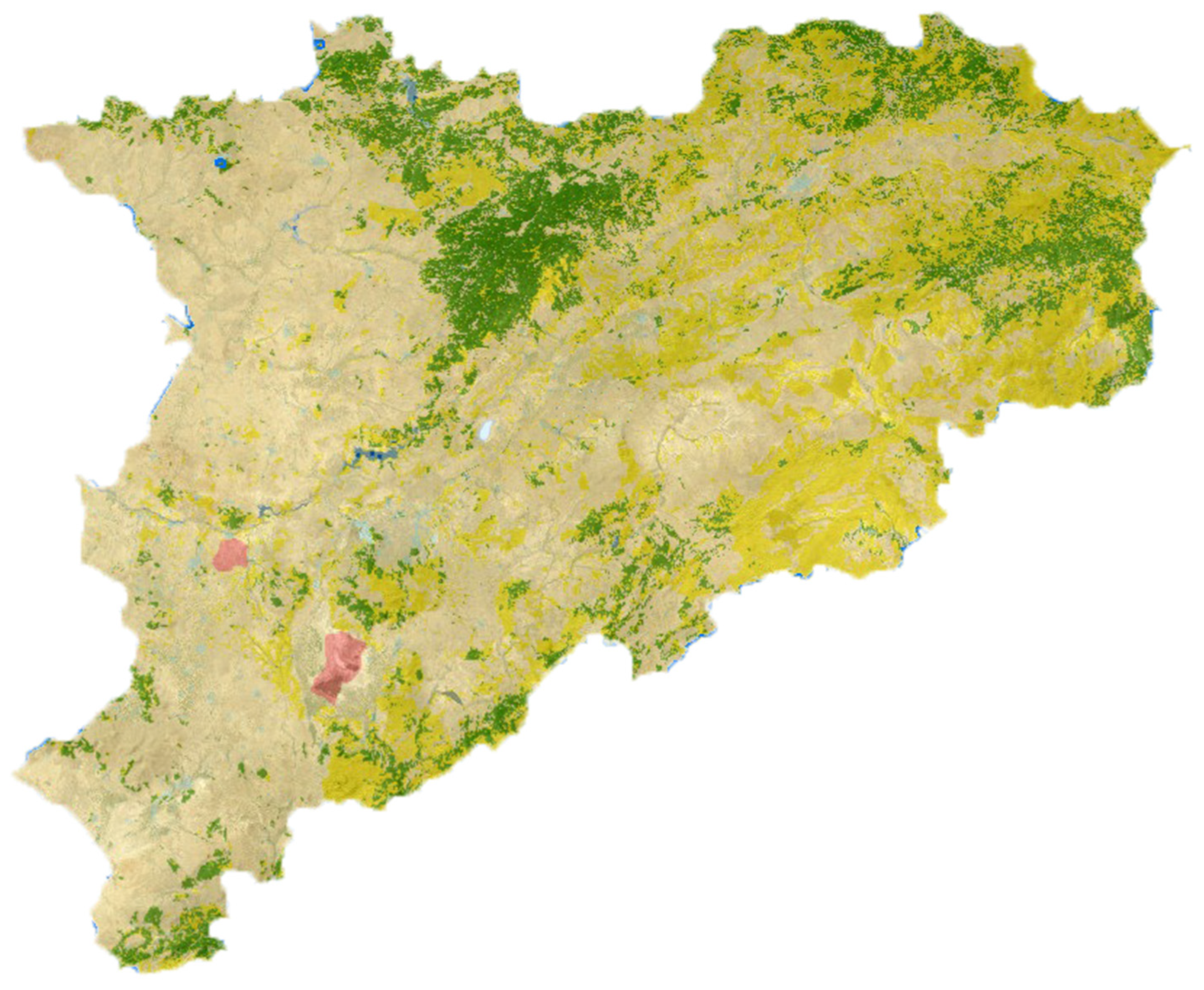
The geographical location of KRDF within Türkiye is shown in Figure 1, and the spatial distribution of forest cover in the country is shown in Figure 2.

2.2. Methods

2.2.1. Study Design

This study is a retrospective analysis of 364 administrative wildfire records from 2016 to 2025. The data were obtained from official fire-response records. No observations were excluded from the primary fire-size analyses solely because fields were identical; the source file lacked unique incident identifiers sufficient to determine whether an identical pair represented duplicate or distinct incidents. A sensitivity analysis excluding one member of the identical pair did not materially change the principal inferential results.

2.2.2. Variable Definitions and Data Quality

Primary outcomes were total burned area (ha) and large-fire status (>5 ha = 1; <=5 ha = 0). Initial response time was recorded in minutes. Recorded ignition cause, calendar season, time-of-day period, and forestry directorate were treated as categorical variables. Month was not entered together with season in multivariable models to avoid redundant temporal parameterization.

The administrative vehicle variable is labeled “number of vehicles used” in the source workbook. Because the dataset does not establish whether this represents the initial dispatch or the total number used during the incident, temporal ordering could not be verified. The variable was therefore summarized descriptively and excluded from predictive/associational regression models. The workbook variable labeled “type” was confirmed from the coding sheet to represent vegetation/land-cover category rather than wildfire behavior type; it was not interpreted as fire type.

Range and consistency checks identified two negative control-duration values and one missing extinguishing-duration value. Negative duration values were treated as invalid and omitted from duration summaries without imputation; control and extinguishing durations were descriptive only and were not included in inferential models. Thirty-one fires had total burned area recorded as the exact numeric value 0.00 ha in the source workbook. The accompanying coding sheet does not define whether 0.00 denotes no measurable spread, rounding below a measurement threshold, or another administrative recording convention; therefore, no specific mechanism was assigned to these values. The zero-area records were distributed as follows: Spring 0/11 (0.0%), Summer 12/182 (6.6%), Autumn 14/162 (8.6%), and Winter 5/9 (55.6%). These observations were retained and modeled explicitly in the first component of the two-part analysis.

2.3. Statistical Analysis

Data management and descriptive checks were performed with IBM SPSS Statistics 22.0. Advanced analyses were conducted in Python 3.13.5 using NumPy 2.3.5, SciPy 1.17.0, statsmodels 0.14.6, and scikit-learn 1.8.0. Continuous variables are reported as mean +/− SD and median (Q1–Q3) where appropriate, and categorical variables as n (%). All tests were two-sided with alpha = 0.05. Logistic-model results are reported as odds ratios (ORs), whereas exponentiated coefficients from the Gamma log-link model are reported as conditional mean ratios (MRs), each with 95% confidence intervals (CIs).

Annual trends in fire count, mean burned area, mean initial response time, and large-fire percentage were evaluated with Kendall’s tau and Sen’s slope. Because the 2025 mean response time was visibly lower than preceding years, a post hoc sensitivity analysis repeated the response-time trend after excluding 2025. LOESS curves were retained for descriptive visualization only.

Large-fire status (>5 ha) was analyzed with Firth-penalized logistic regression because only 56 large fires were observed and complete separation occurred in sparse seasonal categories. The model included initial response time and categorical terms for season, ignition cause, time of day, and forestry directorate. Summer, negligence/carelessness, 12:01–16:00, and Kayseri were reference categories. With 17 predictor parameters and 56 events, the events-per-parameter ratio was 3.29; penalized estimation was therefore used to reduce small-sample bias and obtain finite estimates under separation [34]. For Firth models, Wald standard errors were obtained from the inverse expected information matrix evaluated at the Firth estimates; two-sided Wald p-values were calculated from z = beta/SE, and 95% Wald CIs for ORs were obtained as exp(beta +/− 1.96 × SE). The apparent AUC of the multivariable model was reported descriptively.

Burned area was analyzed with a two-part (hurdle) strategy. Part 1 modeled positive versus zero burned area using Firth-penalized logistic regression, retaining all 364 records. Part 2 modeled positive burned area (n = 333) with a Gamma generalized linear model and log link; heteroskedasticity-consistent HC3 standard errors were used. The same covariates and reference categories were used in both primary components. Because only 31 zero-area observations were available relative to 17 predictor parameters in the primary Part 1 model, a reduced Firth sensitivity model was also fitted with initial response time and season only (four predictor parameters; 31 zero-area observations, or 7.75 zero observations per predictor parameter). This reduced specification was used to assess whether the winter association was robust to substantially lower model dimensionality. The positive-area seasonal distribution was Spring n = 11, Summer n = 170, Autumn n = 148, and Winter n = 4.

Receiver operating characteristic analysis was used only as an exploratory assessment of initial response time as a stand-alone classifier for large fires. The AUC and a stratified bootstrap 95% CI (5000 resamples; seed = 20,260,718) were calculated. Youden’s J was used to identify the dataset-specific threshold with the highest combined sensitivity and specificity; this value was not interpreted as a universal operational cutoff.

Seasonal burned-area distributions were compared with the Kruskal–Wallis test. Effect size was summarized with epsilon-squared and a 5000-resample bootstrap 95% CI. Pairwise season comparisons used Mann–Whitney U tests with Holm correction. Bootstrap 95% CIs for seasonal medians and Wilson 95% CIs for large-fire proportions are described in Section 3.5.

3. Results

A total of 364 wildfire records were analyzed. Mean burned area was 2.81 +/− 5.13 ha and the median was 1.00 ha (Q1–Q3: 0.17–2.93), confirming a markedly right-skewed distribution. Mean initial response time was 20.12 +/− 14.11 min (median 16.00 min). After excluding two invalid negative control-duration values, valid control-duration data were available for 362 fires (395.17 +/− 669.49 min; median 165 min). Extinguishing duration was available for 363 fires (2160.52 +/− 5159.74 min; median 1155 min) (

Table 1. Descriptive statistics for continuous variables.

Variable	n	Mean +/− SD	Median	Q1	Q3	Min	Max
Burned area (ha)	364	2.81 +/− 5.13	1.00	0.17	2.93	0.00	46.40
Initial response time (min)	364	20.12 +/− 14.11	16.00	15.00	23.25	0.00	209.00
Control duration (min)	362	395.17 +/− 669.49	165.00	75.00	349.50	10.00	6050.00
Extinguishing duration (min)	363	2160.52 +/− 5159.74	1155.00	336.00	2651.50	20.00	89,580.00
Vehicles used	364	2.52 +/− 2.84	2.00	1.00	3.00	0.00	28.00

Note: Negative control-duration values (n = 2) were treated as invalid and excluded from duration summaries. Extinguishing duration had one missing value. Vehicle count is reported descriptively only because the source variable denotes vehicles used and does not establish initial-dispatch timing.

).

Fifty-six fires (15.4%) exceeded 5 ha, and 31 fires had a recorded burned area of 0 ha. The recorded cause was negligence/carelessness in 333 fires (91.5%), natural event in 16, accident in 13, and re-ignition in two. The administrative vehicle count averaged 2.52 +/− 2.84 (median 2; range 0–28) but was not used as an inferential predictor because its timing relative to the incident could not be verified.

3.1. Trend Analysis (2016–2025)

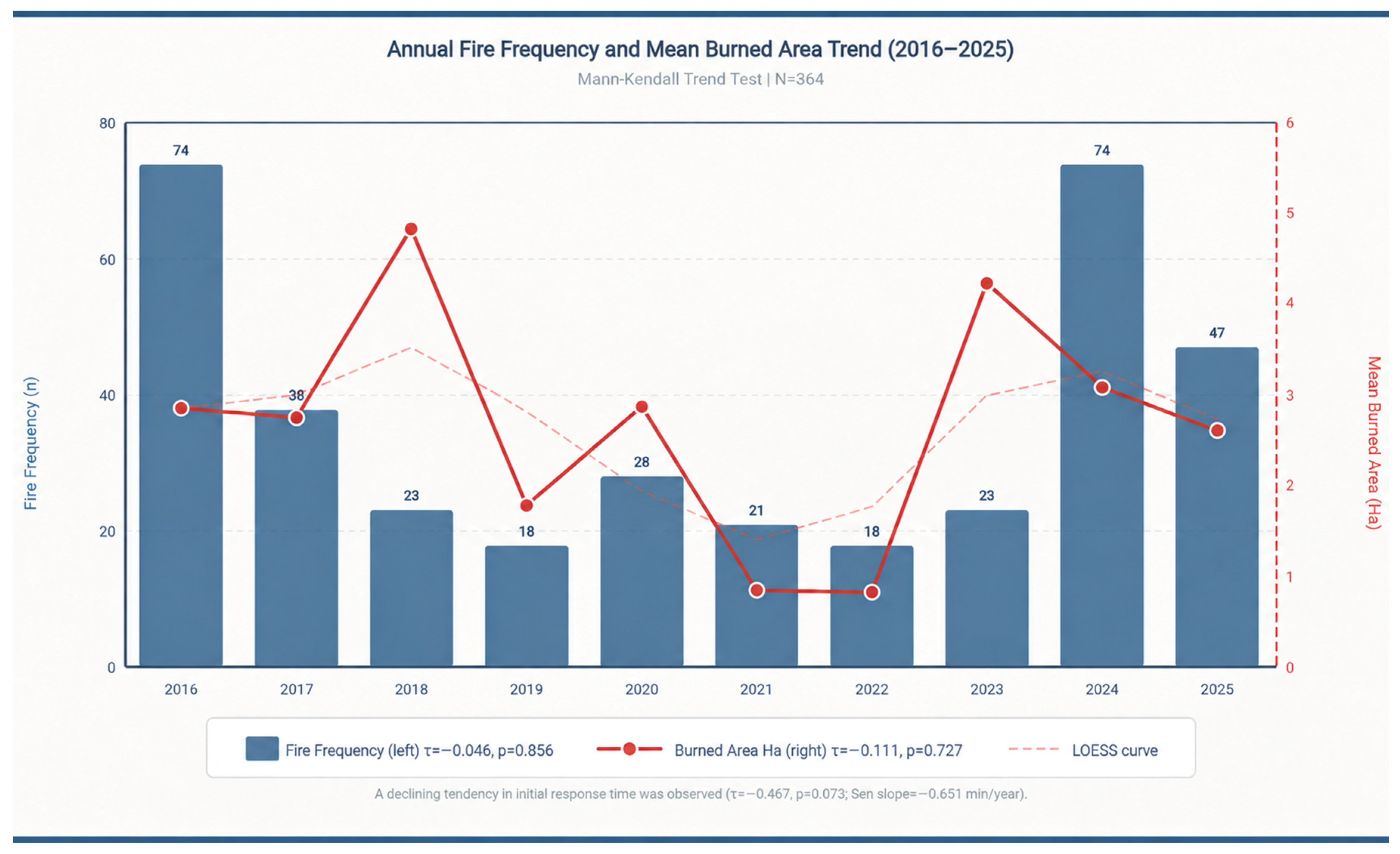
No statistically significant monotonic trend was detected for annual fire count (tau = −0.046, p = 0.856), mean burned area (tau = −0.111, p = 0.727), or large-fire percentage (tau = 0.135, p = 0.590) (Figure 3). Mean initial response time showed a decreasing tendency (tau = −0.467, p = 0.073; Sen slope = −0.651 min/year), but this did not meet the prespecified significance threshold (Table 2).

Figure 3. Annual number of fires (bars, left axis) and mean burned area (dotted line, right axis). The LOESS smoothing curve is displayed with a dashed line.

Figure 3. Annual number of fires (bars, left axis) and mean burned area (dotted line, right axis). The LOESS smoothing curve is displayed with a dashed line.

Table 2. Annual wildfire characteristics and Mann–Kendall trend results.

Year	n	Mean Area (ha)	Median Area (ha)	Mean Response (min)	Large Fire (n)	Large Fire (%)
2016	74	2.86	1.50	22.73	10	13.5
2017	38	2.75	1.25	22.08	3	7.9
2018	23	4.84	3.59	20.30	8	34.8
2019	18	1.79	1.00	17.94	1	5.6
2020	28	2.88	0.71	19.29	4	14.3
2021	21	0.85	0.30	17.10	1	4.8
2022	18	0.84	0.15	17.00	1	5.6
2023	23	4.24	1.75	21.43	4	17.4
2024	74	3.09	0.80	22.04	17	23.0
2025	47	2.61	0.12	14.57	7	14.9
Mann–Kendall tau	−0.046	−0.111	-	−0.467	-	0.135
p	0.856	0.727	-	0.073	-	0.590
Sen slope/year	0.000	−0.028	-	−0.651	-	0.193

Note: Sen’s slope quantifies annual change. The response-time sensitivity analysis excluding 2025 yielded tau = −0.333, p = 0.260 and Sen slope = −0.370 min/year.

Table 2. Annual wildfire characteristics and Mann–Kendall trend results.

Year	n	Mean Area (ha)	Median Area (ha)	Mean Response (min)	Large Fire (n)	Large Fire (%)
2016	74	2.86	1.50	22.73	10	13.5
2017	38	2.75	1.25	22.08	3	7.9
2018	23	4.84	3.59	20.30	8	34.8
2019	18	1.79	1.00	17.94	1	5.6
2020	28	2.88	0.71	19.29	4	14.3
2021	21	0.85	0.30	17.10	1	4.8
2022	18	0.84	0.15	17.00	1	5.6
2023	23	4.24	1.75	21.43	4	17.4
2024	74	3.09	0.80	22.04	17	23.0
2025	47	2.61	0.12	14.57	7	14.9
Mann–Kendall tau	−0.046	−0.111	-	−0.467	-	0.135
p	0.856	0.727	-	0.073	-	0.590
Sen slope/year	0.000	−0.028	-	−0.651	-	0.193

Note: Sen’s slope quantifies annual change. The response-time sensitivity analysis excluding 2025 yielded tau = −0.333, p = 0.260 and Sen slope = −0.370 min/year.

Sensitivity analysis excluding 2025 attenuated the response-time trend (tau = −0.333, p = 0.260; Sen slope = −0.370 min/year), indicating that the low 2025 mean contributed materially to the apparent decline. Accordingly, the temporal pattern was not interpreted as evidence of operational improvement.

The highest annual fire count was shared by 2016 and 2024 (n = 74 each). The highest observed large-fire percentage occurred in 2018 (34.8%; 8/23), not 2024. These year-specific fluctuations were descriptive and did not constitute a statistically significant long-term trend.

The corrected multivariable large-fire model used categorical coding for season, cause, time of day, and forestry directorate and excluded the ambiguous vehicle-count variable. The model contained 17 predictor parameters for 56 large-fire events (events per parameter = 3.29). Its apparent AUC was 0.703; this value should not be interpreted as externally validated predictive performance.

3.2. Firth-Penalized Logistic Regression for Large Fire

No predictor reached statistical significance in the Firth model. Initial response time was not independently associated with large-fire odds (OR = 1.007 per minute, 95% CI 0.989–1.026; p = 0.452). Autumn versus summer was also not significant for the binary >5 ha outcome (OR = 1.338, 95% CI 0.747–2.397; p = 0.328) (

Table 3. Firth-penalized logistic regression for large-fire status (>5 ha), N = 364.

Predictor	Beta	SE	OR (95% CI)	p
Initial response time (per min)	0.007	0.009	1.007 (0.989–1.026)	0.452
Season: Spring vs. Summer	−1.750	1.492	0.174 (0.009–3.232)	0.241
Season: Autumn vs. Summer	0.291	0.298	1.338 (0.747–2.397)	0.328
Season: Winter vs. Summer	−1.410	1.513	0.244 (0.013–4.735)	0.351
Cause: Natural event vs. Negligence/carelessness	−0.012	0.742	0.988 (0.231–4.231)	0.987
Cause: Accident vs. Negligence/carelessness	−1.789	1.474	0.167 (0.009–3.002)	0.225
Cause: Re-ignition vs. Negligence/carelessness	1.542	1.491	4.673 (0.251–86.823)	0.301
Time: 08:00–12:00 vs. 12:01–16:00	−0.899	0.607	0.407 (0.124–1.339)	0.139
Time: 16:01–20:00 vs. 12:01–16:00	−0.554	0.371	0.575 (0.278–1.189)	0.135
Time: 20:01–08:00 vs. 12:01–16:00	0.115	0.632	1.122 (0.325–3.876)	0.855
Directorate: Akdagmadeni vs. Kayseri	0.057	0.496	1.059 (0.400–2.801)	0.909
Directorate: Cayiralan vs. Kayseri	−0.904	0.617	0.405 (0.121–1.356)	0.143
Directorate: Nevsehir vs. Kayseri	0.638	0.547	1.892 (0.648–5.531)	0.244
Directorate: Nigde vs. Kayseri	−1.312	0.703	0.269 (0.068–1.069)	0.062
Directorate: Sivas vs. Kayseri	−0.539	0.454	0.583 (0.240–1.419)	0.235
Directorate: Yozgat vs. Kayseri	−0.009	0.758	0.991 (0.224–4.375)	0.990
Directorate: Zara vs. Kayseri	−0.240	0.475	0.786 (0.310–1.996)	0.613

Note: OR = odds ratio; CI = confidence interval. Reference categories: Summer; negligence/carelessness; 12:01–16:00; Kayseri. The model included 17 predictor parameters and 56 events (events per parameter = 3.29). Apparent AUC = 0.703. Vehicle count was excluded because initial-dispatch timing could not be verified.

).

The wide CIs for sparse categories, especially spring, winter, re-ignition, and some directorates, indicate substantial uncertainty. These estimates were therefore treated as associative and exploratory rather than as stable prediction coefficients.

3.3. Two-Part Model for Burned Area

Part 1 distinguished zero from positive burned area using Firth logistic regression. Initial response time was not associated with the odds of a positive burned area (OR = 0.990, 95% CI 0.972–1.009; p = 0.297). Winter had lower odds of a positive recorded burned area than summer (OR = 0.067, 95% CI 0.015–0.300; p < 0.001), but the winter sample was small (n = 9) and this estimate should be interpreted cautiously. Zero-area records occurred in 0/11 spring fires, 12/182 summer fires, 14/162 autumn fires, and 5/9 winter fires. In the reduced Firth sensitivity model containing only initial response time and season, the winter association was materially unchanged (Winter vs. Summer OR = 0.065, 95% CI 0.015–0.275; p < 0.001). Initial response time remained nonsignificant (OR = 0.986, 95% CI 0.968–1.004; p = 0.117), as did Spring vs. Summer (OR = 1.769, 95% CI 0.087–35.959; p = 0.710) and Autumn vs. Summer (OR = 0.805, 95% CI 0.362–1.792; p = 0.595) (Table 4). Thus, the winter estimate was robust to the reduced specification, although its interpretation remains limited by the very small winter sample and the uncertain recording mechanism for values of 0.00 ha.

Table 4. Two-part model for burned area: positive-area occurrence and positive burned-area magnitude.

Predictor	Part 1 OR (95% CI)	p	Part 2 MR (95% CI)	p
Initial response time (per min)	0.990 (0.972–1.009)	0.297	1.012 (0.998–1.026)	0.097
Season: Spring vs. Summer	1.434 (0.084–24.373)	0.803	0.493 (0.189–1.286)	0.148
Season: Autumn vs. Summer	0.833 (0.386–1.795)	0.640	1.683 (1.233–2.295)	0.001
Season: Winter vs. Summer	0.067 (0.015–0.300)	<0.001	0.455 (0.222–0.932)	0.031
Cause: Natural event vs. Negligence/carelessness	2.815 (0.175–45.184)	0.465	1.007 (0.490–2.071)	0.984
Cause: Accident vs. Negligence/carelessness	1.968 (0.116–33.392)	0.639	0.300 (0.128–0.700)	0.005
Cause: Re-ignition vs. Negligence/carelessness	0.442 (0.009–21.943)	0.682	1.820 (0.405–8.179)	0.435
Time: 08:00–12:00 vs. 12:01–16:00	0.532 (0.159–1.776)	0.305	0.490 (0.299–0.802)	0.005
Time: 16:01–20:00 vs. 12:01–16:00	0.632 (0.272–1.470)	0.287	0.481 (0.341–0.678)	<0.001
Time: 20:01–08:00 vs. 12:01–16:00	0.924 (0.203–4.202)	0.918	0.598 (0.294–1.217)	0.156
Directorate: Akdagmadeni vs. Kayseri	0.724 (0.170–3.090)	0.663	0.534 (0.284–1.003)	0.051
Directorate: Cayiralan vs. Kayseri	0.914 (0.241–3.465)	0.895	0.585 (0.343–0.996)	0.048
Directorate: Nevsehir vs. Kayseri	3.352 (0.217–51.742)	0.386	1.434 (0.859–2.392)	0.168
Directorate: Nigde vs. Kayseri	0.426 (0.134–1.355)	0.148	0.549 (0.257–1.171)	0.121
Directorate: Sivas vs. Kayseri	0.555 (0.199–1.549)	0.261	0.655 (0.436–0.983)	0.041
Directorate: Yozgat vs. Kayseri	1.104 (0.155–7.844)	0.921	1.840 (0.682–4.959)	0.228
Directorate: Zara vs. Kayseri	1.527 (0.356–6.554)	0.569	0.835 (0.493–1.412)	0.501

Note: Part 1 = Firth logistic regression for positive versus zero burned area (N = 364). Part 2 = Gamma GLM with log link and HC3 robust SE for positive burned area (N = 333). OR/MR estimates are adjusted for all variables shown. Reference categories: Summer; negligence/carelessness; 12:01–16:00; Kayseri. Vehicle count was excluded. MR = conditional mean ratio for positive burned area.

Table 4. Two-part model for burned area: positive-area occurrence and positive burned-area magnitude.

Predictor	Part 1 OR (95% CI)	p	Part 2 MR (95% CI)	p
Initial response time (per min)	0.990 (0.972–1.009)	0.297	1.012 (0.998–1.026)	0.097
Season: Spring vs. Summer	1.434 (0.084–24.373)	0.803	0.493 (0.189–1.286)	0.148
Season: Autumn vs. Summer	0.833 (0.386–1.795)	0.640	1.683 (1.233–2.295)	0.001
Season: Winter vs. Summer	0.067 (0.015–0.300)	<0.001	0.455 (0.222–0.932)	0.031
Cause: Natural event vs. Negligence/carelessness	2.815 (0.175–45.184)	0.465	1.007 (0.490–2.071)	0.984
Cause: Accident vs. Negligence/carelessness	1.968 (0.116–33.392)	0.639	0.300 (0.128–0.700)	0.005
Cause: Re-ignition vs. Negligence/carelessness	0.442 (0.009–21.943)	0.682	1.820 (0.405–8.179)	0.435
Time: 08:00–12:00 vs. 12:01–16:00	0.532 (0.159–1.776)	0.305	0.490 (0.299–0.802)	0.005
Time: 16:01–20:00 vs. 12:01–16:00	0.632 (0.272–1.470)	0.287	0.481 (0.341–0.678)	<0.001
Time: 20:01–08:00 vs. 12:01–16:00	0.924 (0.203–4.202)	0.918	0.598 (0.294–1.217)	0.156
Directorate: Akdagmadeni vs. Kayseri	0.724 (0.170–3.090)	0.663	0.534 (0.284–1.003)	0.051
Directorate: Cayiralan vs. Kayseri	0.914 (0.241–3.465)	0.895	0.585 (0.343–0.996)	0.048
Directorate: Nevsehir vs. Kayseri	3.352 (0.217–51.742)	0.386	1.434 (0.859–2.392)	0.168
Directorate: Nigde vs. Kayseri	0.426 (0.134–1.355)	0.148	0.549 (0.257–1.171)	0.121
Directorate: Sivas vs. Kayseri	0.555 (0.199–1.549)	0.261	0.655 (0.436–0.983)	0.041
Directorate: Yozgat vs. Kayseri	1.104 (0.155–7.844)	0.921	1.840 (0.682–4.959)	0.228
Directorate: Zara vs. Kayseri	1.527 (0.356–6.554)	0.569	0.835 (0.493–1.412)	0.501

Note: Part 1 = Firth logistic regression for positive versus zero burned area (N = 364). Part 2 = Gamma GLM with log link and HC3 robust SE for positive burned area (N = 333). OR/MR estimates are adjusted for all variables shown. Reference categories: Summer; negligence/carelessness; 12:01–16:00; Kayseri. Vehicle count was excluded. MR = conditional mean ratio for positive burned area.

Among the 333 fires with positive burned area, the Gamma component showed that autumn fires had a larger conditional mean burned area than summer fires (MR = 1.683, 95% CI 1.233–2.295; p = 0.001). In contrast, initial response time was not statistically significant after adjustment (MR = 1.012 per minute, 95% CI 0.998–1.026; p = 0.097). Thus, the earlier interpretation of a 2.6% increase in burned area per additional minute was not retained in the corrected primary model.

Other associations in the positive-area Gamma component included a lower conditional mean burned area for accident versus negligence/carelessness (MR = 0.300, p = 0.005), 08:00–12:00 versus 12:01–16:00 (MR = 0.490, p = 0.005), and 16:01–20:00 versus 12:01–16:00 (MR = 0.481, p < 0.001). Directorate estimates also showed heterogeneity, with Cayiralan (MR = 0.585, p = 0.048) and Sivas (MR = 0.655, p = 0.041) lower than Kayseri. These results are associative and may reflect unmeasured environmental, access, or incident-severity differences.

The primary two-part model intentionally excluded vehicle count. A sensitivity analysis excluding one member of the identical-record pair produced materially unchanged estimates for initial response time (Gamma MR = 1.012, p = 0.091) and autumn versus summer (MR = 1.687, p = 0.001).

3.4. Exploratory ROC Analysis

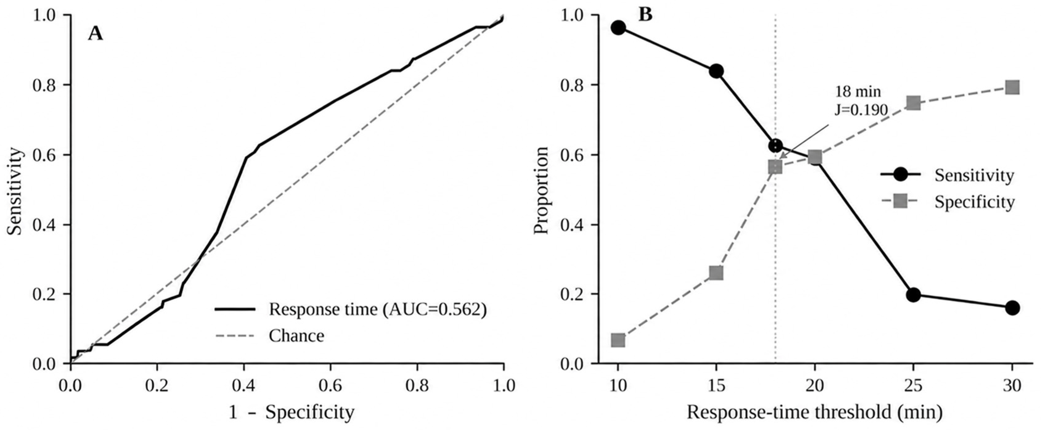
Initial response time alone weakly discriminated large fires (>5 ha), with AUC = 0.562 (stratified bootstrap 95% CI 0.489–0.636). This AUC is distinct from the apparent AUC of the full Firth model (0.703) and confirms that response time by itself is not a reliable classifier.

The threshold maximizing Youden’s J in this dataset was 18 min (sensitivity = 0.625, specificity = 0.565, J = 0.190) (Figure 4). Because both discrimination and J were weak, 18 min was treated only as a dataset-specific monitoring reference and not as a target, safety standard, or deterministic decision boundary.

Figure 4. (A) ROC curve for initial response time as a stand-alone classifier of large fire (AUC = 0.562; 95% bootstrap CI 0.489–0.636). (B) Sensitivity and specificity across selected thresholds. The 18 min value maximized Youden J (0.190) in this dataset but is not an operational cutoff.

Figure 4. (A) ROC curve for initial response time as a stand-alone classifier of large fire (AUC = 0.562; 95% bootstrap CI 0.489–0.636). (B) Sensitivity and specificity across selected thresholds. The 18 min value maximized Youden J (0.190) in this dataset but is not an operational cutoff.

Threshold comparisons illustrate the expected sensitivity–specificity trade-off: lower response-time thresholds increased sensitivity at the cost of very low specificity, whereas higher thresholds increased specificity while missing more large fires (

Table 5. Exploratory response-time thresholds for large-fire classification.

Threshold (min)	Sensitivity	Specificity	1-Specificity	Youden J	Interpretation
10	0.964	0.065	0.935	0.029	Very low specificity
15	0.839	0.260	0.740	0.099	Low specificity
18	0.625	0.565	0.435	0.190	Highest J in dataset
20	0.589	0.594	0.406	0.183	Similar trade-off
25	0.196	0.747	0.253	−0.057	Very low sensitivity
30	0.161	0.792	0.208	−0.047	Very low sensitivity

Note: The 18 min value is the threshold with the highest Youden J in this dataset only. AUC = 0.562 (95% bootstrap CI 0.489–0.636); therefore, no threshold is recommended as an operational cutoff.

).

The ROC findings were considered supplementary and were not used to support causal claims or prescriptive response-time targets.

3.5. Seasonal Differences

Burned-area distributions differed across the four calendar seasons (Kruskal–Wallis H = 12.759, df = 3, p = 0.005). The effect size was small (epsilon-squared = 0.027; 95% bootstrap CI 0.003–0.081) (Table 6).

Table 6. Burned area and large-fire frequency by corrected calendar season.

Season	n	Median Area (ha)	Mean Area (ha)	Large Fire (%)	Large Fire (n)
Spring	11	0.75	1.53	0.0	0
Summer	182	0.73	2.22	14.3	26
Autumn	162	1.47	3.67	18.5	30
Winter	9	0.00	0.78	0.0	0
Global test	H = 12.759	df = 3	p = 0.005	epsilon-squared = 0.027	95% CI 0.003–0.081

Note: Seasons were defined as Spring = March–May, Summer = June–August, Autumn = September–November, Winter = December–February. Global Kruskal–Wallis H = 12.759, df = 3, p = 0.005; epsilon-squared = 0.027 (95% bootstrap CI 0.003–0.081). Holm-corrected post hoc: Autumn vs. Summer p = 0.035; all other pairs p > 0.05.

Table 6. Burned area and large-fire frequency by corrected calendar season.

Season	n	Median Area (ha)	Mean Area (ha)	Large Fire (%)	Large Fire (n)
Spring	11	0.75	1.53	0.0	0
Summer	182	0.73	2.22	14.3	26
Autumn	162	1.47	3.67	18.5	30
Winter	9	0.00	0.78	0.0	0
Global test	H = 12.759	df = 3	p = 0.005	epsilon-squared = 0.027	95% CI 0.003–0.081

Note: Seasons were defined as Spring = March–May, Summer = June–August, Autumn = September–November, Winter = December–February. Global Kruskal–Wallis H = 12.759, df = 3, p = 0.005; epsilon-squared = 0.027 (95% bootstrap CI 0.003–0.081). Holm-corrected post hoc: Autumn vs. Summer p = 0.035; all other pairs p > 0.05.

After Holm correction, only the autumn-versus-summer pairwise comparison remained statistically significant (adjusted p = 0.035). Spring versus summer did not differ (adjusted p = 0.998). Thus, the previous “spring paradox” interpretation resulted from incorrect season labels and was removed.

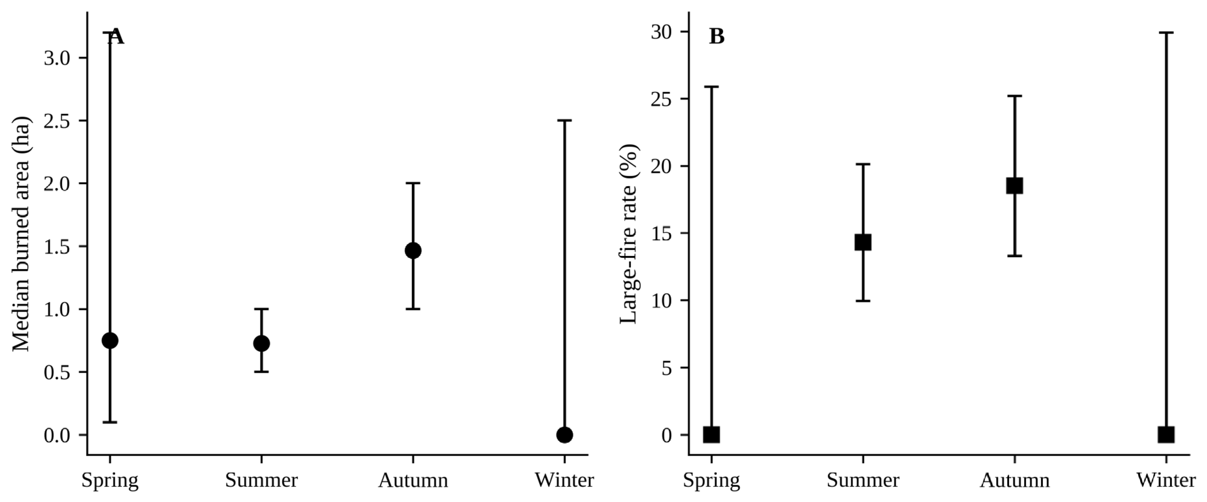
The corrected seasonal distribution was Spring n = 11 (median 0.75 ha; mean 1.53 ha; 0 large fires), Summer n = 182 (median 0.73 ha; mean 2.22 ha; 26 large fires, 14.3%), Autumn n = 162 (median 1.47 ha; mean 3.67 ha; 30 large fires, 18.5%), and Winter n = 9 (median 0.00 ha; mean 0.78 ha; 0 large fires) (Figure 5).

Figure 5. (A) Median burned area by corrected calendar season with bootstrap 95% CIs. (B) Large-fire rate with Wilson 95% CIs. Autumn had the highest median burned area and large-fire proportion; the corrected Gamma model estimated an Autumn vs. Summer MR = 1.683 (p = 0.001).

Figure 5. (A) Median burned area by corrected calendar season with bootstrap 95% CIs. (B) Large-fire rate with Wilson 95% CIs. Autumn had the highest median burned area and large-fire proportion; the corrected Gamma model estimated an Autumn vs. Summer MR = 1.683 (p = 0.001).

For the positive-area Gamma component, the seasonal sample was Spring n = 11, Summer n = 170, Autumn n = 148, and Winter n = 4 after the 31 zero-area observations were separated into Part 1 of the two-part model.

4. Discussion

4.1. Principal Findings

The revised analysis changes the central interpretation of the study. After correcting season labels, treating categorical variables appropriately, excluding an ambiguously timed vehicle variable from inferential models, and addressing zero burned-area observations with a two-part approach, the strongest reproducible pattern was seasonal rather than a response-time effect. Autumn, not spring, was associated with greater positive burned area than summer. Initial response time was not significant in either the Firth large-fire model or the adjusted positive-area Gamma model.

4.2. Seasonal Pattern and the Two-Part Burned-Area Model

The corrected calendar coding showed that most fires occurred in summer and autumn, consistent with the regional description of concentration in summer and early autumn [30,31]. Autumn had a higher median burned area than summer and remained associated with a greater conditional mean positive burned area in the Gamma component (MR = 1.683). The global seasonal effect was statistically significant but small (epsilon-squared = 0.027), and only Autumn vs. Summer remained significant after Holm correction. These results support regional seasonal heterogeneity but not a broad claim that spring is the dominant risk period.

Potential explanations for the autumn pattern include late-season fuel dryness, agricultural activity, and persistent heat or drought conditions; however, none of these mechanisms were measured directly. Mediterranean evidence shows that heatwaves, drought, and fire activity can co-occur and interact [35], but the present data cannot attribute the observed seasonal association to a specific meteorological process. The very small spring and winter samples also limit precision.

Separating zero burned-area incidents from positive burned area was important because the 31 records were explicitly stored as 0.00 ha in the source workbook rather than as missing values. However, the source documentation does not indicate whether these values represent no measurable spread, rounding below a measurement threshold, or another administrative convention, so the underlying recording mechanism cannot be determined from the available data. The concentration of zero-area records in winter (5/9) contributed to the lower odds of positive burned area in that season. Importantly, a reduced Firth model containing only initial response time and season yielded a nearly identical Winter vs. Summer estimate (OR = 0.065, 95% CI 0.015–0.275; p < 0.001), supporting robustness to lower model dimensionality while not resolving the uncertainty created by the small winter sample. The second component quantified differences in the magnitude of positive area. This two-part structure avoids deleting zero-area records before modeling while keeping their recording uncertainty explicit.

4.3. Response Time, Accessibility, and Operational Interpretation

Response time alone had weak discriminatory ability for large fires (AUC = 0.562), and the corrected multivariable analyses did not show an independent association at the 0.05 level. In the positive-area Gamma model, the estimate corresponded to an MR of 1.012 per additional minute (p = 0.097), substantially weaker than the previously reported 2.6% increase. This result does not imply that response time is operationally irrelevant. Rather, response time can be influenced by road access, distance from response bases, terrain, concurrent incidents, and fire behavior at detection [14,18,19]. Without these covariates, it should be interpreted as a composite operational indicator and possible proxy for accessibility or remoteness.

The vehicle-count variable illustrates a related problem. The source workbook labels it as the number of vehicles used, not unequivocally the number initially dispatched. Total resources used can increase in response to a difficult or expanding fire, creating confounding by indication and reverse temporal ordering. Suppression systems can also select which fires remain observable as larger events, a broader phenomenon discussed as suppression bias [36]. For these reasons, vehicle count was retained descriptively but removed from the revised inferential models.

4.4. Large-Fire Modeling and Thresholds

Only 56 fires exceeded 5 ha. Correct dummy coding generated 17 predictor parameters, corresponding to 3.29 events per parameter, and sparse seasonal/cause categories produced separation. Firth penalization was therefore appropriate to obtain finite, bias-reduced estimates [34]. No individual predictor reached statistical significance, and several CIs were wide. These results should be interpreted as evidence of uncertainty rather than evidence that the corresponding factors have no operational importance.

The contrast between the binary large-fire outcome and continuous burned area is still informative, but the revised interpretation is more cautious than the original manuscript. A fixed >5 ha threshold compresses outcome information, while the two-part model preserves the distinction between zero spread and the magnitude of positive spread. The response-time-only ROC analysis further demonstrates that a single operational variable cannot reliably separate large from smaller fires in this dataset.

The 18 min value should therefore not be used as an operational target. Its Youden J was only 0.190, and its AUC was close to chance. At most, it describes the point that maximized sensitivity plus specificity in this particular sample. Operational standards should instead be based on validated multi-factor models and agency-specific performance objectives.

4.5. Temporal Trends and Sensitivity Analysis

The 2016–2025 series did not show statistically significant monotonic trends in fire count, mean burned area, large-fire percentage, or response time. The apparent decline in mean response time was sensitive to the low 2025 value; when 2025 was omitted, tau changed from −0.467 (p = 0.073) to −0.333 (p = 0.260). Accordingly, the data do not support describing the period as a demonstrated operational success, and unmeasured technological investments, UAV use, smoke sensors, or decision-support systems should not be invoked as explanations.

Annual peaks also require descriptive caution. Fire count was tied at 74 in 2016 and 2024, while the highest large-fire percentage occurred in 2018 (34.8%), not 2024. This variability reinforces the need to distinguish individual high-activity years from statistically supported long-term trends.

4.6. Spatial Context, Resilience, and Data Limitations

The dataset does not directly measure governance quality, municipal capacity, social vulnerability, economic effects, ecosystem services, WUI configuration, or land-use exposure. Consequently, these concepts should be treated as interpretive context rather than measured outcomes. Spatial-planning research demonstrates the value of integrating ecosystem information into territorial decision-making [6], and WUI mapping can identify fine-scale variation in wildfire exposure [7]. Future analyses in KRDF would be strengthened by incident coordinates, roads, station locations, settlement proximity, WUI metrics, and travel-time surfaces.

The most important omitted covariates are meteorological and biophysical: wind speed, relative humidity, temperature, drought indices, slope, aspect, fuel continuity, distance to the responding unit, and fire size or behavior at detection. Their absence creates potential omitted-variable bias in all operational associations. The revised manuscript therefore uses association language throughout and does not interpret model coefficients as causal effects.

Additional limitations include sparse spring and winter observations, administrative coding that may not capture incident complexity, invalid values in post-event duration fields, and the absence of unique incident identifiers. One pair of records was identical across available fields; excluding one record in sensitivity analysis did not materially change the key Gamma or Firth results. The study also lacks an external validation dataset, so discrimination estimates are descriptive rather than transportable prediction metrics.

4.7. Practical Implications

The findings support three practical priorities. First, seasonal preparedness should reflect the observed summer–autumn concentration and the greater positive burned area observed in autumn. Second, response time should continue to be monitored as an operational performance indicator, but without treating 18 min as a universal target or assuming a causal effect on final area. Third, future decision support should combine operational records with weather, fuel, terrain, access, and spatial exposure data; resource positioning and routing methods are most informative when these dimensions are integrated rather than considered in isolation.

5. Conclusions

This 10-year administrative wildfire dataset shows that corrected calendar season is associated with burned-area magnitude, with autumn fires having a greater conditional mean positive burned area than summer fires after multivariable adjustment. In contrast, initial response time was not independently associated with large-fire odds or positive burned-area magnitude in the conservative revised models. The large-fire Firth model contained no statistically significant individual predictor, and response time alone had weak discriminatory ability. The 18 min ROC value should therefore be regarded only as a dataset-specific exploratory reference, not an operational cutoff. The results support continued seasonal preparedness and response-time monitoring while underscoring the need to integrate meteorological, fuel, terrain, accessibility, distance, and incident-at-detection information in future analyses. Because governance, WUI configuration, social vulnerability, and ecosystem-service outcomes were not directly measured, these remain directions for future integrated research rather than outcomes demonstrated by the present dataset.

The empirical findings therefore support seasonal heterogeneity but do not support a causal response-time effect, a universal 18 min cutoff, or direct claims about governance performance. These results are best interpreted as an operational analysis of administrative wildfire records. More informative risk models will require incident-level meteorology, fuels, terrain, access, distance, fire conditions at detection, and geospatial exposure indicators.

For practice, the data justify continued monitoring of response processes and autumn preparedness, while emphasizing that operational decisions should be based on multivariable, locally validated information rather than a single threshold. For research, linking administrative response records with WUI, road-network, fuel, weather, and land-use data is the most important next step.