Abstract
Harmonizing economic growth and carbon emissions is key to reaching the “dual carbon” targets. This research centers on the seven key urban agglomerations within the Yellow River Basin (YRB) and establishes an integrated research framework of decoupling effect quantification–spatial association recognition–driving factor analysis. By combining the Tapio decoupling model, a modified gravity model, social network analysis (SNA), and the Logarithmic Mean Divisia Index (LMDI) method, the study systematically evaluates the decoupling states, spatial association structure, and driving mechanisms between regional carbon emissions and economic growth from 2001 to 2020. The results show that: (1) All seven urban agglomerations exhibit a simultaneous upward trend in both carbon emissions and GDP, but significant regional disparities exist, with some agglomerations demonstrating a green growth pattern where economic growth outpaces carbon emissions. (2) Weak decoupling is the predominant type among urban agglomerations and their constituent cities in the YRB. Notably, some regions have regressed to growing connection or growing negative decoupling during 2016–2020. (3) The spatial network of carbon emission decoupling effects exhibits a core-periphery structure characterized by stronger eastern regions and weaker western regions, with the Shandong Peninsula and Guanzhong Plain urban agglomerations serving as core nodes for regional linkage. (4) Per capita GDP and technological level play a dominant role in promoting decoupling, while energy intensity and the population carrying intensity of the real economy are the primary inhibiting factors; the impact of industrial structure shows an unstable direction. Grounded in these findings, this study formulates differentiated carbon reduction pathways tailored to regional heterogeneity, providing theoretical insights and actionable guidance to facilitate the low-carbon transition and coordinated governance of urban agglomerations.
1. Introduction
Global concern regarding climate change and carbon emissions has intensified in recent years. Accelerated industrial and urban development has led to a substantial increase in carbon emissions, which has had a significant effect on the global climate [1]. The United Nations has promoted global cooperation on emission reduction through international frameworks such as the Paris Agreement, while the IPCC has continuously called for urgent action based on scientific assessments [2]. The international community has widely recognized the urgency of controlling carbon emissions and addressing climate change [3]. China, being the most populous nation and the second-largest economy, ranked first globally in carbon emissions in 2019 [4]. In September 2020, the Chinese government officially announced its commitment to the international community to accomplish the “dual carbon” objectives [5]. Pursuing a low-carbon transition and meeting carbon reduction targets poses a major challenge to China’s pursuit of sustainable development [6]. Urban agglomerations, as advanced regional spatial forms emerging in the process of industrialization and urbanization, play a central role in tackling climate change and advancing the low-carbon transition. They are characterized by a high concentration of economic activity and population [7]. As of 2021, China’s 19 urban agglomerations, occupying 25% of the land area, concentrated 75% of the total population and generated 80% of the national GDP, but they also caused ecological degradation and substantial carbon emissions [8]. Therefore, uncovering the linkage between economic progress and carbon emissions decoupling, spatial association characteristics, and driving factors at the urban agglomeration scale is crucial for achieving the “dual carbon” goals.
The Yellow River has a watershed area accounting for 8.3% of China’s total land area [9,10]. Fossil energy resources, including coal, petroleum, and coalbed methane, are abundant in the YRB, which has evolved into a key hub for China’s energy, chemical, and heavy industry production during its economic development. Under China’s strategic layout of the “5 + 1” energy bases, three energy bases are located within the YRB, resulting in the region exhibiting concentrated pollution and emission characteristics. Comprehensive watershed management and sustainable development aimed at carbon reduction have become important breakthrough approaches to coordinate the regional conflict between protection and development. The exploration of carbon emission decoupling dynamics and drivers in the YRB, together with the formulation of precise carbon reduction measures, is of considerable practical importance for implementing the national strategy and achieving the dual carbon goals. To better capture the dynamic linkage between economic growth and carbon emissions, researchers have introduced the concept of decoupling [11], which was originally used to describe the degree of independence between variables. If no dependency is observed between the variables, it is considered that “decoupling” has been achieved [12]. The Organisation for Economic Co-operation and Development (OECD) introduced decoupling theory as a core framework for analyzing whether economic growth and resource consumption evolve synchronously [13]. Tapio [14] proposed the decoupling elasticity index—overcoming the OECD index’s base-year limitations—to systematically examine how economic growth and environmental decoupling interact. This model effectively mitigates measurement distortions from base-year selection and is widely employed to quantify carbon-economy decoupling dynamics across diverse regions and sectors [15,16,17]. Complementing aggregate intensity indices, micro-scale models leveraging driving-behavior features and machine learning can explain and predict vehicle fuel use and CO2 emissions, offering bottom-up evidence to validate city-level trends [18,19].
As carbon emission governance has shifted from total quantity control to efficiency improvement and structural optimization, increasing attention has been paid to the spatial linkage characteristics of carbon emissions across regions [20]. In existing studies, traditional methods such as Exploratory Spatial Data Analysis, Classical Spatial Data Analysis, and spatial econometrics can reveal local spatial clustering or spatial lag effects of carbon emission activities. However, these methods largely rely on the assumption of geographical proximity, which constrains the identification of multidirectional and asymmetric spatial dependencies among cities. Moreover, they are limited in capturing the network structure characteristics of interregional carbon emission interactions [21]. To address these limitations, researchers have increasingly adopted SNA in studies on carbon reduction [22]. The SNA method not only considers the spatial connections between cities but also accounts for the interactions between each city’s own characteristics and their relationships. It can explicitly illustrate the overall pattern and key nodes of the regional system in the form of a network structure, thereby more comprehensively revealing the structural features and evolutionary paths in the carbon emission linkage process [23]. However, current research largely emphasizes identifying spatial patterns of overall carbon emissions or energy flows, yet the combined use of SNA and models like the gravity model to reveal the spatial characteristics of the decoupling effect is still underdeveloped. At the scale of urban agglomerations, research on the spatial network characteristics and evolution of carbon decoupling remains insufficient, hindering efforts to support coordinated regional emission reduction and policy integration.
Further identifying the driving mechanisms of carbon emission decoupling effects can inform the development of tailored and region-specific mitigation policies. Current methods for identifying carbon emission drivers predominantly comprise Structural Decomposition Analysis and Index Decomposition Analysis (IDA) [24,25,26], among which IDA has been widely applied due to its low data requirements and strong explanatory power [27]. Within this framework, the LMDI method proposed by Ang et al. [28], with advantages such as zero residuals, strong additivity, and negative values, has emerged as a key approach for analyzing the determinants of carbon emissions. Drawing on the Kaya identity, the approach attributes variations in carbon emissions to specific factors [29,30]. Although some studies have integrated decomposition analysis with decoupling theory [31,32], most have focused on the provincial or city level, lacking systematic research on entire urban agglomerations within river basins and their dynamic evolutionary processes. This limitation makes it difficult to provide strong support for formulating differentiated low-carbon policies in the YRB.
In light of the issues and limitations mentioned above, this study constructs an integrated analytical framework centered on decoupling effect quantification–spatial association recognition–driving factor analysis. Employing the Tapio decoupling framework, this study measures decoupling states between carbon emissions and economic output in the seven key urban agglomerations. The spatial coupling relationships and core nodes among urban agglomerations are identified using a modified gravity model in combination with SNA. Using LMDI decomposition, we isolate key determinants of carbon decoupling heterogeneity across urban agglomerations. Providing conceptual underpinnings for green restructuring and high-value development in the YRB, this study also provides policy-relevant implications for other developing countries and regions in formulating differentiated carbon reduction policies. This study makes the following three marginal contributions beyond the existing literature: (1) Through a comparative analysis of urban agglomerations, this research uncovers the dynamics of carbon and economic decoupling in the YRB, establishing an evidence base for regionally tailored climate governance. (2) Utilizing the modified gravity model and SNA, this study establishes a spatial association framework for analyzing carbon emission decoupling effects, identifies core nodes and network hierarchy, and expands the spatial structural dimension of carbon decoupling research. (3) In the decomposition of driving factors, this study innovatively introduces the indicator of “population carrying intensity of the real economy” to quantify the impact of spatial matching between population and industry on carbon decoupling, providing a new perspective for a more comprehensive understanding of the linkage mechanism between human–industry coupling and carbon reduction.
2. Materials and Methods
2.1. Study Area
The YRB spans nine provinces across eastern, central, and western China, covering a total area of approximately 795,000 km2 [33]. It serves as the core area of the national “Two Screens and Three Belts” ecological security pattern in the upper reaches, an energy and chemical industry base in the middle reaches, and a major grain-producing region in the lower reaches. However, the YRB exhibits ecological fragility, driven by both natural climatic variability and intensified anthropogenic disturbances. The upper reaches have experienced a decline in water conservation capacity due to overgrazing and other factors. The middle reaches suffer from serious soil erosion and water pollution, while the lower reaches face river channel disconnection and wetland shrinkage. The YRB is rich in resources such as coal, oil, and natural gas, earning it the title of China’s Energy Basin [34,35]. In addition, the YRB also possesses abundant hydropower and wind energy resources, providing a strong energy foundation for high-quality economic development.
The YRB constitutes a key area characterized by high population density and substantial economic activity in China [36], comprising seven major urban agglomerations (Figure 1). These urban agglomerations encompass sixty-nine prefecture-level cities (Appendix A, Table A1) and form the forefront of promoting ecological sustainability and regional development in the YRB. By 2022, the seven urban agglomerations in the YRB were home to approximately 270 million people, comprising around 64% of the basin’s total population. These regions collectively contributed nearly 70% of the YRB’s total GDP.
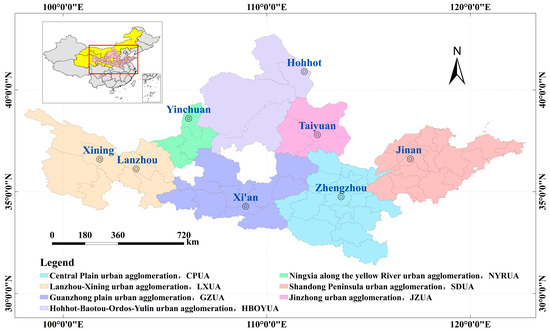
Figure 1.
Urban agglomerations and prefecture-level administrative divisions in the YRB.
2.2. Data
This study mainly uses data on carbon emissions and socioeconomic indicators. City-level carbon emissions data for 2001–2020 were obtained from the China Emissions Accounts and Datasets (CEADs, version 2023) carbon accounting database. The CEADs dataset constructs city-level emission inventories by integrating official energy balance tables with socio-economic statistics at the prefecture level. Emissions from different fuel types are allocated to cities according to industrial output, energy consumption, and population data, ensuring consistency and comparability across years. To address gaps in city-level energy statistics, CEADs employed night-time light imagery for spatial downscaling: DMSP/OLS data for 2001–2013 and NPP/VIIRS data for 2014–2020, thereby improving the spatial accuracy of city-level CO2 estimates. This dataset, which leverages the aforementioned night-time light data for spatial refinement, has found broad application in carbon emissions research [37,38]. In this study, we directly used the processed city-level data without further downscaling. At the urban agglomeration scale, carbon emissions were aggregated directly by summing the values of the 69 prefecture-level cities within the seven YRB urban agglomerations (Appendix A, Table A1), based on their administrative boundaries, with no additional spatial interpolation to ensure full consistency with official administrative units.
The socioeconomic statistical data include energy consumption data, GDP, population, urbanization rate, industrial structure, and other indicators for each prefecture-level administrative unit. Data were primarily drawn from the China City Statistical Yearbook, as well as the Energy and Industrial Statistical Yearbooks of China, and the statistical yearbooks of various provinces and regions. For missing data, weighted averages or linear interpolation methods were used for estimation. All GDP data used in this study were adjusted to constant prices with 2000 as the base year to eliminate the effect of inflation. The GDP deflator was derived from the China Statistical Yearbook and provincial statistical yearbooks, specifically from the indicator “Gross Regional Product Index.” Accordingly, all annual GDP values were converted into 2000 constant prices. For consistency, all GDP-related indicators—including carbon intensity (carbon emissions/GDP), Tapio decoupling elasticity, and Per Capita GDP in the LMDI decomposition—were uniformly calculated using 2000 constant-price GDP, ensuring comparability across years and regions.
2.3. Methods
2.3.1. Analytical Framework
As shown in Figure 2, the research framework comprises four key components: (1) Revealing the spatiotemporal evolution characteristics of carbon emissions and GDP; (2) Adopting the Tapio index for quantifying the decoupling dynamics between economic activity and carbon emissions; (3) Constructing a spatial network of decoupling effects by integrating the modified gravity model and SNA; (4) Identifying key drivers of carbon emission decoupling using the LMDI decomposition model.
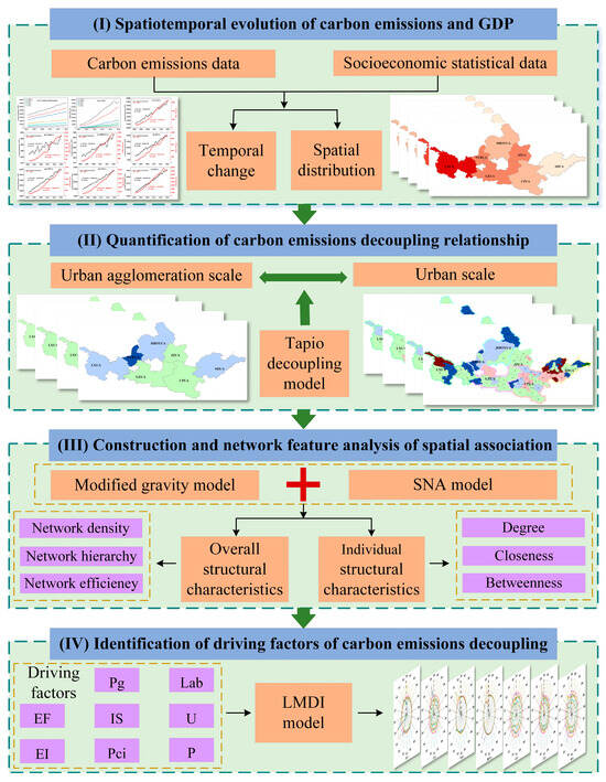
Figure 2.
Methodological framework.
2.3.2. Quantification Method of Carbon Emission Decoupling
Carbon emission decoupling denotes the ideal weakening and eventual break of the association between CO2 emissions and economic development. In this context, carbon emissions remain stable or even decline while economic growth continues. This research establishes the Tapio decoupling framework to quantify the dynamics of decoupling between carbon emissions and economic growth across seven major urban agglomerations and individual cities. The model formulation is presented below:
In the equation, reflects the extent to which carbon emissions are decoupled from GDP growth and denote the growth rates of carbon emissions and GDP over the study period, respectively. and correspond to carbon emission values at the start and conclusion of the study period, ∆C, and signifies the net increment. , , and ∆GDP represent the GDP during the study period’s beginning and end, and the GDP increment during the study period, respectively. Referring to China’s five-year economic development plans, this study divides the entire research period (2001–2020) into four sub-periods: 2001–2005, 2006–2010, 2011–2015, and 2016–2020.
Following existing research [39,40] and variations in carbon emissions, GDP, and the decoupling index, this study identifies eight distinct states of decoupling between carbon emissions and the economy (Figure 3 and Appendix A, Table A2). For robustness, we reclassified the decoupling types using alternative Tapio thresholds (0.75/1.25), and the results (Appendix B, Table A8) were nearly identical to the current results, confirming the stability of the classification.
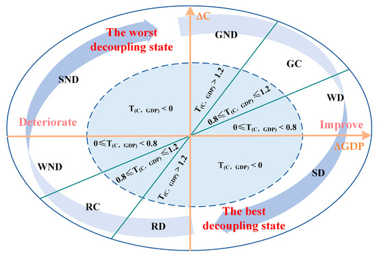
Figure 3.
Quadrant diagram for decoupling state classification.
2.3.3. Recognition Method for Spatial Association Characteristics in Carbon Emission Decoupling Effects
To explore the spatial characteristics of carbon emission decoupling effects among urban agglomerations in the YRB, this study applies a modified gravity model [41] integrated with SNA [42]. Firstly, the spatial association matrix of carbon emission decoupling is constructed using the modified gravity model. Subsequently, to analyze the spatial association features of carbon emission decoupling effects among urban agglomerations in the YRB, this study applies the SNA method from two perspectives: the overall and individual structural features.
The modified gravity model operates based on the following principle:
In the formula, represents the spatial association strength of the carbon emission decoupling link between region i and region j. denotes the contribution coefficient of region i to the spatial association strength of the carbon emission decoupling link between regions i and j, which serves as the modified gravity exponent. This adjustment overcomes the limitation of the traditional gravity model, where the gravity exponent is fixed at 1, leading to inaccurate estimation results. and represent the resident population of regions i and j. and denote the carbon emission decoupling elasticity indices of regions i and j. and refer to the actual GDP of regions i and j. and represent the regional and geographical distance between regions i and j. Finally, and denote the actual per capita GDP of regions i and j, respectively. Detailed definitions, units, and rationales for all variables and exponents used in the modified gravity model are summarized in Appendix A, Table A3.
Based on previous studies [43,44], we further constructed the spatial association network as follows. The modified gravity model yields a continuous weight , for each city/urban agglomeration pair, which is directly used as the edge weight in the spatial association matrix. To highlight the most significant linkages and avoid excessive network density, we applied a binarization rule by retaining only linkages with weights greater than the mean value of all (alternative robustness checks using the median and top-quartile thresholds yielded consistent patterns). Edges below the threshold were set to zero. Given the symmetric formulation of the gravity model, the resulting network is undirected. Therefore, the final spatial network is a weighted–undirected graph, in which edge weights reflect the relative strength of decoupling associations.
In applying SNA to analyze the spatial association of carbon emission decoupling effects, this study adopts three key metrics to characterize the overall structural properties of the network: network efficiency (NE), network hierarchy (NH), and network density (ND). ND characterizes the degree of association in carbon emission decoupling among analytical units (cities/urban agglomerations), with values in the range [0, 1]. Higher ND values signify a stronger potential for coordinated decoupling among the units. NH is used to measure the heterogeneity of decoupling states among analytical units, with values in the range [0, 1]. Higher NH values signify increased disparities in decoupling states across units, indicating a less balanced network structure. NE reflects the transmission efficiency of carbon emission decoupling states among analytical units, with values in the range [0, 1]. Higher NE values reflect more centralized connection paths and lower redundancy within the network, resulting in shorter transmission paths for decoupling states. However, it also implies fewer alternative paths and decreased network stability, which is unfavorable for building a robust regional collaborative emission reduction system. The following model is used:
In the equation, NR denotes the total relationships within the network, NP represents the count of symmetric reachable node pairs, and NL indicates the number of redundant links.
For individual structural characteristics, three indicators are selected: betweenness centrality (BC), closeness centrality (CC), and degree centrality (DC). DC represents the degree of direct association between a given analytical unit and other units, with values in the range [0, 1]. Higher DC values suggest that the unit has more extensive connections within the network and stronger interaction capacity in regional coordinated decoupling. CC measures the proximity of a given analytical unit to other units, with values in the range [0, 1]. Larger CC values imply a more central role of the unit within the network. BC represents the intermediary role of a given analytical unit in the shortest paths between other units, with values in the range [0, 1]. Higher BC values suggest that the unit has stronger control and bridging functions in the transmission of carbon emission decoupling information. The model is defined as follows:
In the equation, refers to the count of regions directly linked to region i; denotes shortest distance between regions i and j; indicates total shortest paths from regions j to k; and refers to the number passing region i.
2.3.4. Driving Factor Decomposition Method for Carbon Emission Decoupling
The LMDI model is applied to examine the drivers behind carbon emission decoupling among urban agglomerations in the YRB. Following references [33,45,46,47,48,49,50,51], carbon emission drivers are categorized into per capita GDP, energy intensity, energy carbon emission coefficient, industrial structure, population carrying intensity of the real economy, technological level, urbanization rate, and population size (Table 1). The model is defined as follows:
In the equation, GDP denotes regional gross domestic product, E denotes energy consumption, C denotes carbon emissions, GIP denotes the output of the secondary industry, denotes the urban population, and P denotes the resident population.

Table 1.
Key factors driving the decoupling of carbon emissions from economic development.
Using the LMDI method, Equation (11) is decomposed without residuals
In the equation, captures the impact of changes in the carbon emission coefficients of various energy types. As these coefficients are generally constant, thus = 0. , , , , , , and represent the variation in carbon emissions resulting from changes in population size, urbanization rate, technological level, population carrying intensity of the real economy, industrial structure, per capita GDP, energy intensity, respectively.
The decoupling effect between carbon emissions and economic development is further decomposed using the model derived from Equation (1), as shown below:
In the equation, , , , , , , and represent the decoupling elasticity indices of population size, urbanization rate, technological level, population carrying intensity of the real economy, industrial structure, per capita GDP, energy intensity, respectively. An increased value of the decoupling elasticity index suggests a more substantial contribution of the corresponding driver to carbon emission decoupling. A positive elasticity value suggests that the factor promotes carbon emission decoupling, while a negative value indicates an inhibitory effect.
3. Results
3.1. Spatiotemporal Evolution of Carbon Emissions and GDP
Figure 4 illustrates the temporal evolution of carbon emissions and GDP in the seven key urban agglomerations of the YRB. Carbon emissions and GDP both showed a fluctuating increase from 2001 to 2020. Over this period, carbon emissions increased most in the SDUA, followed by the CPUA and GZUA, whereas the NYRUA and HBOYUA experienced the smallest growth. GDP growth showed a similar ranking, with the SDUA and CPUA leading, while the NYRUA remained the lowest. Overall, eastern urban agglomerations recorded faster growth in both emissions and GDP than their western counterparts.
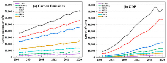
Figure 4.
Temporal evolution of carbon emissions and GDP in YRB urban agglomerations (2001–2020).
To provide a comprehensive characterization of the carbon emissions and GDP dynamics across the seven urban agglomerations, Table 2 presents the variation rates across different periods. The results indicate that the carbon emission growth rates in the LXUA, NYRUA, and HBOYUA exhibited a downward trend followed by an upward shift over time. In contrast, the carbon emission growth rates in the JZUA, GZUA, CPUA, and SDUA exhibited a fluctuating downward trend. Compared to the period from 2001 to 2005, the carbon emission growth rate of the JZUA experienced the largest reduction during 2016–2020, with a decrease of 64.92%. Meanwhile, the GDP growth rates of seven urban agglomerations exhibited a declining trend. The SDUA underwent the most significant decline in GDP growth rate, decreasing from 98.84% (2001–2005) to 10.48% (2016–2020), representing a reduction of 89.39%.
Table 2.
Carbon emissions and GDP growth trends in YRB urban agglomerations by sub-period.
Figure 5 presents the spatiotemporal evolution of carbon emission intensity across YRB urban agglomerations. Spatially, urban agglomerations in the eastern YRB generally exhibit lower carbon emission intensity than those in the west. In five typical years, the SDUA exhibits a carbon emission intensity of less than 4 t/CNY 10,000. Temporally, carbon emission intensity has exhibited a downward trend over the years. By 2020, all urban agglomerations in the YRB had achieved carbon emission intensities lower than 4 t/CNY 10,000, indicating steady progress in energy efficiency and emission reduction, along with a clear move toward low-carbon development. This lays a firm basis for the pursuit of the dual carbon objectives in the YRB. The LXUA experienced the largest reduction in carbon emission intensity, decreasing from 17.70 t/CNY 10,000 in 2001 to 3.87 t/CNY 10,000 in 2020, representing a decline of 78.14%.
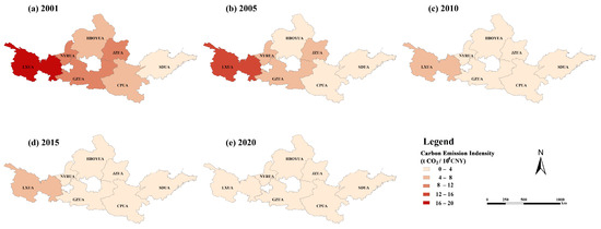
Figure 5.
Spatiotemporal variations in carbon intensity across the YRB urban agglomerations.
3.2. Decoupling Dynamics of Carbon Emissions and Economic Growth
As shown in Figure 6, from 2001 to 2005, WD characterized all major YRB urban agglomerations. In the following two periods (2006–2010 and 2011–2015), this state remained unchanged for most regions, except NYRUA, which shifted to SD. Across the 2016–2020 period, urban agglomerations in the YRB showed pronounced differences in their decoupling states (Appendix A, Table A4). The decoupling states of SDUA, HBOYUA, and LXUA were GC during this period, while NYRUA’s state degraded to GND. The remaining urban agglomerations maintained the WD state. From a temporal perspective, except for HBOYUA and JZUA, the decoupling indices of other urban agglomerations first decreased and then increased, with the lowest values occurring during 2006–2010. It can thus be inferred that, under the current economic development model, the urban agglomerations in the YRB are unlikely to break away from their dependence on fossil fuels, indicating that the path toward carbon emission reduction remains long and challenging.
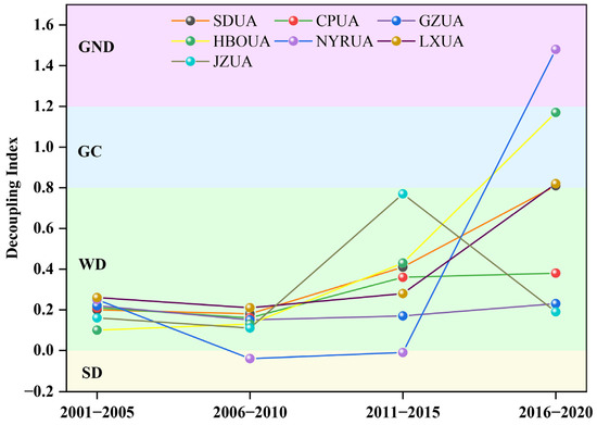
Figure 6.
Decoupling effects at the urban agglomeration scale in the YRB from 2001 to 2020.
Figure 7 illustrates the transition characteristics of city-level decoupling states in the YRB across different periods. It is evident that WD has been the dominant state among cities in YRB urban agglomerations during 2001–2020. In terms of the evolution process, the number of SD cities remained relatively stable at around 10, but their spatial distribution changed significantly (Figure 8). The number of WD cities fluctuated considerably, decreasing from 63 in 2001–2005 to 29 in 2016–2020. Among them, 15.87% shifted to SD, 12.70% to GC, 19.05% to GND, 7.94% to SND, and 1.59% to WND. The number of cities in GC and GND states showed an increasing trend over the years. By 2016–2020, the counts of GC and GND cities had risen to 9 and 14, respectively. Spatially (Figure 8d), GC cities are mainly located in the CPUA, while GND cities are primarily found in the LXUA and SDUA. There is only one WND city, located in the SDUA (Weihai City). Compared to 2001–2005, the number of SND cities increased significantly by 2016–2020, reaching six. These cities are Zibo, Zaozhuang, Dongying, Tai’an, Liaocheng, and Haibei Tibetan Autonomous Prefecture.
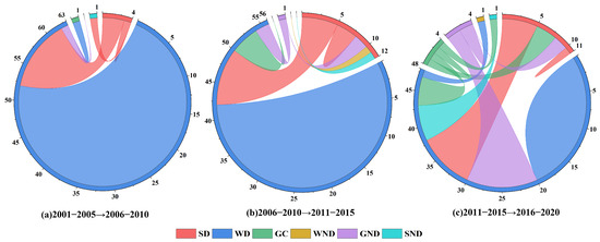
Figure 7.
Transition characteristics of decoupling states in cities of YRB urban agglomerations.
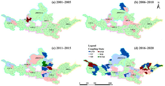
Figure 8.
Spatial pattern of urban scale decoupling states in urban agglomerations of the YRB. City codes are provided in Appendix A, Table A5.
3.3. Spatial Association Characteristics of Carbon Emission Decoupling Effects
Compared with 2001 (Figure 9), the ND of all YRB urban agglomerations increased by 2020, except for NYRUA, indicating a greater degree of internal spatial association of carbon emission decoupling within most agglomerations (Appendix A, Table A6). Nevertheless, the overall ND values remain relatively low, reflecting weak internal linkages and limited cooperation on emission reduction among constituent cities. By contrast, inter-agglomeration ND values are relatively higher, suggesting that cross-agglomeration decoupling associations are stronger than intra-agglomeration ones. Regarding NH, a general downward trend is observed, suggesting a progressive weakening of rigid hierarchical structures and a growing influence of more evenly distributed spatial associations. However, CPUA and NYRUA deviate from this trend, with increasing NH values indicating the persistence of hierarchical dominance by a few core cities. As for NE, values declined overall, reflecting fewer redundant links and the formation of more overlapping and efficient connections as internal cohesion strengthens. This indicates enhanced stability of the spatial association network. Nonetheless, NE values remain above 0.65, pointing to considerable potential for further strengthening both intra-agglomeration and inter-agglomeration decoupling connections. Finally, the number of network contacts generally increased, except in HBOYUA and LXUA, suggesting rising cohesion of decoupling effects within most agglomerations. However, both intra-agglomeration and overall connections remain below their maximum possible levels. For instance, in CPUA, the theoretical maximum number of contacts is 380 (20 × 19), whereas the actual numbers in 2001 and 2020 were 156 and 195, respectively. This gap underscores the continued insufficiency of network density and indicates substantial room for enhancing spatial cooperation on carbon emission decoupling.
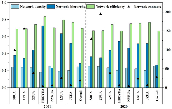
Figure 9.
Overall features of the spatial network representing carbon emission decoupling among urban agglomerations.
From the overall perspective of YRB urban agglomerations, both the DC and CC increased from 2001 (Figure 10a) to 2020 (Figure 10b), whereas BC remained largely unchanged (Appendix A, Table A7). SDUA and GZUA consistently exhibited relatively high values across all three-centrality metrics, suggesting that they function as key hubs in connecting regions and regulating the spatial spillovers of carbon emission decoupling. At the intra-agglomeration level (Figure 10c,d), cities such as Linyi, Weihai, Tai’an, Zhengzhou, Xi’an, Xianyang, and Hainan Tibetan Autonomous Prefecture maintained high DC levels in both 2001 and 2020, indicating that the carbon emission decoupling effects of these cities are tightly linked to others and hold a key position in the overall regional network. Regarding CC, cities including Qingdao, Weihai, Weifang, Zhengzhou, Luoyang, Xi’an, Tongchuan, and Shangluo maintained high CC levels in both 2001 and 2020, showing that they serve as principal hubs in the carbon emission decoupling spatial network and play an essential part in guiding other cities in the diffusion of carbon reduction factors. For BC, cities such as Rizhao, Weihai, Weifang, Zhengzhou, Kaifeng, Xi’an, Baoji, and Shangluo maintained high levels, highlighting their bridging functions within the network and their influence on regional carbon reduction efforts through the mediation of resource flows.
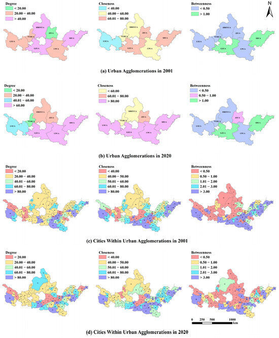
Figure 10.
Individual network characteristics of carbon emission decoupling among urban agglomerations.
3.4. Analysis of the Driving Factors of Carbon Emissions and Economic Growth Decoupling
From the annual changes in the decoupling elasticity indices of driving factors in the YRB urban agglomerations (Figure 11), the key factors influencing decoupling between carbon emissions and economic growth vary across urban agglomerations. From an overall perspective, EI, Pg, Lab, and Pci are the primary drivers affecting the decoupling state. The decoupling elasticity index of Pg exhibited little change, indicating a relatively stable influence on the decoupling of carbon emissions from economic growth. The elasticity indices of the other three main drivers remained generally stable during most periods, although fluctuations occurred in certain years. Changes in the driving factors across the YRB urban agglomerations mainly occurred during 2016–2020. During 2011–2015, HBOYUA showed distinct trends in U and Lab, likely reflecting the region’s transition from a resource-dependent urban economy. Regional industrial expansion attracted rural populations to migrate to urban areas, and there was a lag in technological substitution during the transformation of traditional industries [52]. From 2011 to 2015, EI and IS were the primary inhibitory factors for GZUA and JZUA. This is mainly because both urban agglomerations are important energy and heavy industry bases in China, dominated by traditional industries with high energy consumption, a monotonous energy structure, and inefficient utilization. The industrial similarity among cities within these agglomerations led to overcapacity and inefficient resource allocation.
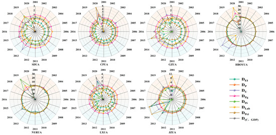
Figure 11.
Temporal variation of the decoupling elasticity index of driving factors in YRB urban agglomerations.
4. Discussion
Focusing on the decoupling between carbon emissions and economic growth in YRB urban agglomerations, this study conducted a systematic analysis of decoupling effects, spatial association structures, and driving factors, laying a foundation for understanding regional heterogeneity and underlying mechanisms. The SDUA has both the largest economic scale and the highest development level, positioning it as a “growth pole” in the YRB. Nevertheless, it is also the largest contributor to carbon emissions. Similarly, carbon emissions in HBOYUA and NYRUA grew rapidly during 2016–2020, reflecting their roles as key energy-rich regions in China. HBOYUA, in particular, served as a national base for advanced energy and chemical industries, relying mainly on coal, oil, and natural gas. Its industrial structure is dominated by secondary, energy-intensive, and pollution-heavy industries. These patterns align with prior studies highlighting the challenges of balancing economic growth and low-carbon transitions in resource-dependent regions [53].
During 2001–2020, the decoupling between economic growth and carbon emissions exhibited considerable instability, with no consistent evolutionary trajectory observed across different scales (Figure 8), which is consistent with the findings of Du et al. [54]. Notably, WD shows the highest persistence across periods, while SD and GND tend to be more transitional. A bipolarization trend emerged after 2011, with GND states expanding rapidly in 2016–2020, especially in SDUA, LXUA, NYRUA, and HBOYUA. This is closely linked to the dominance of high-energy industries, the delayed green transition, and rising energy use from industrial relocation. Such instability in decoupling trajectories has also been reported in other regional contexts [55], suggesting that fluctuations may be a common feature in economies with uneven industrial upgrading. Key indicators further corroborate this: EI increased by 12–17%, IS expanded by 5–10% toward secondary industries, and coal still accounted for about 65–70% of energy consumption in 2020.
The spatial association network results, derived from the modified gravity model and SNA, reveal clear inter-agglomeration linkages in decoupling effects, consistent with Yang et al. [56]. A core–periphery pattern emerges, with SDUA and GZUA showing high DC, CC, and BC, indicating leading roles in coordination and diffusion. Middle-reach and lower-reach cities also exhibit high BC, serving as key connectors. In contrast, western agglomerations such as NYRUA and LXUA remain marginal with weak connectivity, underscoring uneven coordination capacity (Appendix A, Figure A1). Similar core–periphery structures have also been observed in other basin-scale or cross-regional carbon studies [57], highlighting the systemic nature of spatial imbalance.
The analysis of driving factors reveals multidimensional mechanisms shaping decoupling. Pg and Lab are generally positive drivers with large magnitudes, underscoring the roles of economic development and technological progress, consistent with China’s push for green innovation [58]. In contrast, EI and Pci act as major constraints, particularly in central and western resource-based agglomerations, in line with Wang et al. [59]. Regarding Pci, although unconventional, it effectively reflects population pressure relative to industrial output, consistent with the concept of population carrying intensity [60]. Other factors, such as P and U, show limited influence, while IS exhibits region-specific and stage-specific variability. Comparable findings on the heterogeneity of IS and EI impacts can also be found in recent regional carbon studies [61]. Overall, decoupling arises from combined drivers, highlighting the need for regional collaborative optimization to advance low-carbon transition [62].
Drawing on the temporal dynamics of carbon emission and economic growth decoupling, as well as the spatial association structures and driving factors among urban agglomerations, this study proposes targeted policy recommendations for carbon mitigation.
- (1)
- The SDUA and GZUA are high-value carbon emission clusters (Figure 4) and occupy core leading positions within the spatial network, exhibiting strong transmission capabilities. The carbon decoupling of the SDUA is driven by IS and Pci (Figure 11). Efforts should aim at the joint refinement of industrial and energy structures, increasing the share of the tertiary sector, and developing low-carbon, high-value-added industries [63]. As an important industrial base, GZUA should expedite its shift toward a service-oriented economy, optimize the population–industry matching structure, and enhance coordination with eastern regions to achieve green regional linkage [64].
- (2)
- HBOYUA is dominated by coal and heavy industries, with carbon decoupling strongly constrained by Pci (Figure 11) and exhibiting weak spatial connections (Figure 9). Therefore, efforts should focus on transforming and upgrading high-energy-consuming industries such as the chemical, power, and steel sectors to improve the efficiency of green technology utilization. Meanwhile, collaboration with GZUA, LXUA, and other urban agglomerations should be strengthened to improve HBOYUA’s marginal position in the network and enhance its decoupling responsiveness.
- (3)
- The carbon decoupling of LXUA is significantly influenced by EI and IS, with strong internal cohesion but weak external linkages in the spatial network (Figure 10). It is advisable to guide the reform of resource-reliant urban areas while accelerating the deployment of wind and solar power. Moreover, strengthening linkages with GZUA, HBOYUA, and other urban agglomerations can help enhance its network embeddedness and improve its capacity for cross-regional coordinated emission reduction.
- (4)
- CPUA occupies a hub position in the spatial network, connecting eastern and western urban agglomerations and contributing significantly to the spread of carbon decoupling effects (Figure 10). Under the dual control mechanism, it is recommended to leverage economies of scale and innovation advantages to reduce per capita carbon emissions. Node cities such as Zhengzhou and Luoyang should strengthen green technology R&D and spillover effects, enhancing their bridging roles within the network and driving green transitions in surrounding areas.
- (5)
- NYRUA shows sparse connections and a high degree of marginalization in the network (Figure 9), with its carbon decoupling level constrained by IS and Lab. As a national new energy demonstration zone [65], it should prioritize the development of renewable energy sources like wind and solar and promote the integrated development of generation–grid–load–storage systems [66]. Meanwhile, it is essential to strengthen coordination with GZUA and CPUA to gradually enhance its network participation and collaborative capacity.
- (6)
- JZUA has achieved notable results in carbon emission reduction (Figure 5) and holds a sub-core position in the network, demonstrating strong stability and potential for green spillover. It should continue to emphasize both technological innovation and policy guidance, promote clean energy technologies, and accelerate the green transition. At the same time, mechanisms for experience diffusion should be strengthened to enhance its green spillover effect on surrounding urban agglomerations.
5. Conclusions
This study constructs a research framework of decoupling effect quantification–spatial association recognition–driving factor analysis to examine the relationship between carbon emissions and economic growth in the YRB urban agglomerations. The results highlight the complexity of decoupling processes, the heterogeneous roles of driving factors, and the spatially networked nature of regional carbon reduction linkages.
Beyond the empirical patterns, several broader implications emerge. First, the persistence of weak decoupling and the occasional reversion to GC and GND states suggest that a fundamental shift in the development model remains necessary, particularly through accelerating the low-carbon transformation of resource-dependent cities. Second, the “core–periphery” spatial association structure underscores the importance of strengthening cross-regional collaborative governance and enhancing the connectivity of peripheral areas to achieve more balanced and resilient carbon reduction linkages. Third, the differentiated roles of Pg, Lab, EI, and Pci in shaping decoupling effects indicate that policy measures must be tailored to local development stages, resource endowments, and industrial structures, rather than adopting a one-size-fits-all strategy.
At the policy level, these findings provide useful references for designing coordinated regional emission reduction strategies. Specifically, enhancing renewable energy systems, strengthening technological innovation and green spillover effects, and clarifying the functional positioning of urban agglomerations within the carbon decoupling network are critical to advancing the YRB’s transition toward low-carbon and high-quality development.
This study also has limitations. The spatial association analysis relies on a static network, which constrains the exploration of dynamic evolution processes. Meanwhile, the decomposition model may face issues of multicollinearity among influencing factors. Future research could incorporate dynamic network analysis, causal inference, and more systematic decomposition frameworks to capture the temporal progression of decoupling mechanisms and provide deeper insights into the pathways of regional low-carbon transitions.
Author Contributions
Overall design, Z.Z.; methodology, W.W. and J.C.; software, C.H. and L.Y.; formal analysis, L.Z. and X.L.; writing—Original draft preparation, W.W. and J.C.; writing—Review and editing, Z.Z. and G.C.; funding acquisition, L.Z., X.L. and L.Y. All authors have read and agreed to the published version of the manuscript.
Funding
This research was funded by the China National Key R&D Program (2022YFC3201700); Henan Province Science and Technology Research Project (252102320224, 232102111014, 232102321108); National Natural Science Foundation of China (32101591, 52109017, 52322903, 42201097); Water Conservancy Science and Technology Research Project of Henan Provincial Department of Water Resources (GG202541); the Graduate Innovation Ability Improvement Project (NCWUYC-202416039).
Data Availability Statement
The data presented in this study are available on request from the corresponding author.
Acknowledgments
We would like to express our respect and gratitude to the anonymous reviewers and editors for their professional comments and suggestions.
Conflicts of Interest
The authors declare no conflicts of interest.
Abbreviations
| YRB | Yellow River Basin |
| LMDI | Logarithmic Mean Divisia Index |
| SNA | Social Network Analysis |
| LXUA | Lanzhou-Xining Urban Agglomeration |
| NYRUA | Ningxia Along the Yellow River Urban Agglomeration |
| HBOYUA | Hohhot-Baotou-Ordos-Yulin Urban Agglomeration |
| JZUA | Jinzhong Urban Agglomeration |
| GZUA | Hohhot-Baotou-Ordos-Yulin Urban Agglomeration |
| CPUA | Central Plain Urban Agglomeration |
| SDUA | Shandong Peninsula Urban Agglomeration |
| EI | Energy Intensity |
| IS | Industrial Structure |
| Pci | Population Carrying Intensity of the Real Economy |
| P | Population Size |
| SD | Strong Decoupling |
| WD | Weak Decoupling |
| GC | Growing Connection |
| GND | Growing Negative Decoupling |
| WND | Weak Negative Decoupling |
| SND | Strong Negative Decoupling |
| ND | Network Density |
| NH | Network Hierarchy |
| NE | Network Efficiency |
| DC | Degree Centrality |
| CC | Closeness Centrality |
| BC | Betweenness Centrality |
| Pg | Per Capita GDP |
| Lab | Technological Level |
| U | Urbanization Rate |
Appendix A
Table A1.
Division of the seven urban agglomerations in the YRB.
Table A1.
Division of the seven urban agglomerations in the YRB.
| Abbreviations of Urban Agglomeration Name | Composition of Cities | Number of Cities |
|---|---|---|
| SDUA | Heze, Binzhou, Liaocheng, Dezhou, Linyi, Rizhao, Weihai, Tai’an, Jining, Weifang, Yantai, Dongying, Zaozhuang, Zibo, Qingdao, Jinan | 16 |
| CPUA | Jincheng, Changzhi, Jiyuan, Zhuzhou, Zhoukou, Xinyang, Shangqiu, Nanyang, Sanmenxia, Luohe, Xuchang, Puyang, Jiaozuo, Xinxiang, Hebi, Anyang, Pingdingshan, Luoyang, Kaifeng, Zhengzhou | 20 |
| GZUA | Linfen, Yuncheng, Qingyang, Pingliang, Tianshui, Shangluo, Weinan, Xianyang, Baoji, Tongchuan, Xi’an | 11 |
| HBOYUA | Hohhot, Baotou, Ordos, Yulin | 4 |
| NYRUA | Zhongwei, Wuzhong, Shizuishan, Yinchuan | 4 |
| LXUA | Huangnan Tibetan Autonomous Prefecture, Haibei Tibetan Autonomous Prefecture, Hainan Tibetan Autonomous Prefecture, Haidong, Xining, Linxia Hui Autonomous Prefecture, Dingxi, Baiyin, Lanzhou | 9 |
| JZUA | Taiyuan, Jinzhong, Xinzhou, Lüliang, Yangquan | 5 |
Table A2.
Criteria for classifying decoupling states between carbon emissions and economic development.
Table A2.
Criteria for classifying decoupling states between carbon emissions and economic development.
| Decoupling Types | Decoupling States | ∆GDP | ∆C | Decoupling Index | Interpretation of Decoupling States |
|---|---|---|---|---|---|
| Decoupling | SD | >0 | <0 | (−∞, 0) | The ideal scenario is an increase in economic level accompanied by a decrease in carbon emissions |
| WD | >0 | >0 | [0, 0.8) | The economic growth rate exceeds the carbon emission growth rate | |
| RD | <0 | <0 | (1.2, +∞) | The slowdown in economic growth is smaller than the slowdown in carbon emissions | |
| Connection | GC | >0 | >0 | [0.8, 1.2] | The growth rate of economic level is comparable to the growth rate of carbon emissions |
| RC | <0 | <0 | [0.8, 1.2] | The decline rate of economic level is comparable to the decline rate of carbon emissions | |
| Negative Decoupling | GND | >0 | >0 | (1.2, +∞) | The growth rate of the economic level is slower than the growth rate of carbon emissions |
| WND | <0 | <0 | [0, 0.8) | The rate of economic decline is greater than the rate of carbon emission decline | |
| SND | <0 | >0 | (−∞, 0) | Economic decline coupled with an increase in carbon emissions is the least ideal scenario |
Table A3.
Definitions, units, and justification of parameters in the modified gravity model.
Table A3.
Definitions, units, and justification of parameters in the modified gravity model.
| Symbol | Definition | Unit | Rationale/Justification |
|---|---|---|---|
| CDij | Carbon decoupling linkage strength between city/urban agglomeration i and j | Dimensionless (relative value) | Used as edge weight in the spatial association matrix for SNA analysis |
| rij | Gravity coefficient (contribution ratio of city i in the i-j linkage) | Dimensionless | Reflects the similarity of decoupling states between two regions, amplifying (if close) or attenuating (if divergent) their linkage strength. Derived from Tapio decoupling indicators; normalized to [0, 1] |
| Pi, Pj | Resident population at year-end | 104 persons | Together with per capita GDP, approximates regional economic size; commonly adopted as the “mass” term in gravity models |
| Gi, Gj | Actual gross domestic product (GDP) | 100 million CNY | Serves as an indicator of regional economic development, which drives carbon emissions and affects decoupling processes |
| gi, gj | Per capita GDP (constant price) | CNY per person | Multiplied by population to approximate GDP; adjusted to constant prices to ensure comparability |
| xi, xj | Tapio decoupling index | Dimensionless | Core linkage variable: Directly quantifies the carbon decoupling level of cities |
| Dij | Regional distance (non-spatial resistance) | Dimensionless | Represents institutional or economic structure differences, i.e., non-geographical friction. Constructed from socioeconomic heterogeneity measures |
| dij | Geographical distance | Kilometer (km) | Calculated as centroid-to-centroid great-circle distance between cities/urban agglomerations; classical friction term |
Table A4.
Shares of decoupling states across urban agglomerations in the YRB (%).
Table A4.
Shares of decoupling states across urban agglomerations in the YRB (%).
| Period | SD | WD | GC | GND | WND | SND | |
|---|---|---|---|---|---|---|---|
| SDUA | 2001–2005 | 0.00 | 100.00 | 0.00 | 0.00 | 0.00 | 0.00 |
| 2006–2010 | 0.00 | 100.00 | 0.00 | 0.00 | 0.00 | 0.00 | |
| 2011–2015 | 0.00 | 100.00 | 0.00 | 0.00 | 0.00 | 0.00 | |
| 2016–2020 | 18.75 | 18.75 | 0.00 | 25.00 | 6.25 | 31.25 | |
| CPUA | 2001–2005 | 5.00 | 95.00 | 0.00 | 0.00 | 0.00 | 0.00 |
| 2006–2010 | 20.00 | 80.00 | 0.00 | 0.00 | 0.00 | 0.00 | |
| 2011–2015 | 20.00 | 60.00 | 10.00 | 5.00 | 0.00 | 5.00 | |
| 2016–2020 | 25.00 | 40.00 | 30.00 | 5.00 | 0.00 | 0.00 | |
| GZUA | 2001–2005 | 0.00 | 100.00 | 0.00 | 0.00 | 0.00 | 0.00 |
| 2006–2010 | 18.18 | 81.82 | 0.00 | 0.00 | 0.00 | 0.00 | |
| 2011–2015 | 18.18 | 72.73 | 0.00 | 9.09 | 0.00 | 0.00 | |
| 2016–2020 | 9.09 | 72.73 | 9.09 | 9.09 | 0.00 | 0.00 | |
| HBOYUA | 2001–2005 | 0.00 | 100.00 | 0.00 | 0.00 | 0.00 | 0.00 |
| 2006–2010 | 25.00 | 50.00 | 0.00 | 25.00 | 0.00 | 0.00 | |
| 2011–2015 | 25.00 | 50.00 | 0.00 | 25.00 | 0.00 | 0.00 | |
| 2016–2020 | 0.00 | 25.00 | 25.00 | 50.00 | 0.00 | 0.00 | |
| NYRUA | 2001–2005 | 25.00 | 50.00 | 0.00 | 0.00 | 0.00 | 25.00 |
| 2006–2010 | 75.00 | 25.00 | 0.00 | 0.00 | 0.00 | 0.00 | |
| 2011–2015 | 50.00 | 50.00 | 0.00 | 0.00 | 0.00 | 0.00 | |
| 2016–2020 | 0.00 | 25.00 | 25.00 | 50.00 | 0.00 | 0.00 | |
| LXUA | 2001–2005 | 22.22 | 66.67 | 11.11 | 0.00 | 0.00 | 0.00 |
| 2006–2010 | 11.11 | 88.89 | 0.00 | 0.00 | 0.00 | 0.00 | |
| 2011–2015 | 11.11 | 77.78 | 11.11 | 0.00 | 0.00 | 0.00 | |
| 2016–2020 | 0.00 | 44.44 | 0.00 | 44.44 | 0.00 | 11.11 | |
| JZUA | 2001–2005 | 0.00 | 100.00 | 0.00 | 0.00 | 0.00 | 0.00 |
| 2006–2010 | 20.00 | 80.00 | 0.00 | 0.00 | 0.00 | 0.00 | |
| 2011–2015 | 20.00 | 20.00 | 20.00 | 20.00 | 20.00 | 0.00 | |
| 2016–2020 | 20.00 | 80.00 | 0.00 | 0.00 | 0.00 | 0.00 |
Table A5.
City codes and corresponding city names.
Table A5.
City codes and corresponding city names.
| Code | City Name | Code | City Name | Code | City Name | Code | City Name | Code | City Name |
|---|---|---|---|---|---|---|---|---|---|
| 0 | Shizuishan | 1 | Wuzhong | 2 | Yinchuan | 3 | Zhongwei | 4 | Baoji |
| 5 | Linfen | 6 | Pingliang | 7 | Qingyang | 8 | Shangluo | 9 | Tianshui |
| 10 | Tongchuan | 11 | Weinan | 12 | Xi’an | 13 | Xianyang | 14 | Yuncheng |
| 15 | Baotou | 16 | Ordos | 17 | Hohhot | 18 | Yulin | 19 | Jinzhong |
| 20 | Lüliang | 21 | Taiyuan | 22 | Xinzhou | 23 | Yangquan | 24 | Baiyin |
| 25 | Dingxi | 26 | Haibei Tibetan Autonomous Prefecture | 27 | Haidong | 28 | Hainan Tibetan Autonomous Prefecture | 29 | Huangnan Tibetan Autonomous Prefecture |
| 30 | Lanzhou | 31 | Linxia Hui Autonomous Prefecture | 32 | Xining | 33 | Binzhou | 34 | Dezhou |
| 35 | Dongying | 36 | Heze | 37 | Jinan | 38 | Liaocheng | 39 | Linyi |
| 40 | Qingdao | 41 | Rizhao | 42 | Tai’an | 43 | Weihai | 44 | Weifang |
| 45 | Yantai | 46 | Zaozhuang | 47 | Zibo | 48 | Jining | 49 | Anyang |
| 50 | Hebi | 51 | Jiyuan | 52 | Jiaozuo | 53 | Jincheng | 54 | Kaifeng |
| 55 | Luoyang | 56 | Luohe | 57 | Nanyang | 58 | Pingdingshan | 59 | Puyang |
| 60 | Sanmenxia | 61 | Shangqiu | 62 | Xinxiang | 63 | Xinyang | 64 | Xuchang |
| 65 | Changzhi | 66 | Zhoukou | 67 | Zhumadian | 68 | Zhengzhou | - | - |
Table A6.
ND, NH, and NE of each urban agglomeration in the YRB for 2001, 2010, and 2020.
Table A6.
ND, NH, and NE of each urban agglomeration in the YRB for 2001, 2010, and 2020.
| Urban Agglomeration | 2001 | 2010 | 2020 | ||||||
|---|---|---|---|---|---|---|---|---|---|
| ND | NH | NE | ND | NH | NE | ND | NH | NE | |
| SDUA | 0.2432 | 0.3810 | 0.6910 | 0.2482 | 0.3738 | 0.6813 | 0.2538 | 0.3658 | 0.6705 |
| CPUA | 0.2411 | 0.3450 | 0.6939 | 0.2459 | 0.3486 | 0.6833 | 0.2513 | 0.3525 | 0.6715 |
| GZUA | 0.2355 | 0.4444 | 0.7424 | 0.2415 | 0.4473 | 0.7228 | 0.2345 | 0.4404 | 0.7424 |
| HBOYUA | 0.1833 | 0.7264 | 0.8363 | 0.1936 | 0.6407 | 0.7409 | 0.2051 | 0.5454 | 0.6667 |
| NYRUA | 0.2535 | 0.2333 | 0.7038 | 0.2533 | 0.3376 | 0.6931 | 0.2333 | 0.4669 | 0.7532 |
| LXUA | 0.1947 | 0.6357 | 0.7974 | 0.2082 | 0.5796 | 0.7779 | 0.2233 | 0.5172 | 0.7563 |
| JZUA | 0.2035 | 0.5213 | 0.7665 | 0.2136 | 0.5266 | 0.7738 | 0.2051 | 0.5197 | 0.7663 |
| Overall | 0.2452 | 0.2857 | 0.6967 | 0.2504 | 0.2749 | 0.6782 | 0.2543 | 0.2687 | 0.6667 |
Table A7.
Centrality metrics of the carbon emission decoupling spatial association network by urban agglomeration in the YRB.
Table A7.
Centrality metrics of the carbon emission decoupling spatial association network by urban agglomeration in the YRB.
| Urban Agglomeration | 2001 | 2020 | ||||
|---|---|---|---|---|---|---|
| DC | CC | BC | DC | CC | BC | |
| SDUA | 83.33 | 75.82 | 5.87 | 83.33 | 85.71 | 7.44 |
| CPUA | 33.33 | 48.71 | 0.38 | 83.33 | 83.57 | 0.42 |
| GZUA | 83.33 | 78.84 | 5.44 | 83.33 | 85.71 | 5.97 |
| HBOYUA | 83.33 | 55.55 | 0.19 | 33.33 | 60.22 | 0.14 |
| NYRUA | 33.33 | 43.75 | 0.11 | 16.33 | 42.85 | 0.08 |
| LXUA | 33.33 | 33.92 | 0.18 | 53.33 | 81.54 | 0.22 |
| JZUA | 16.33 | 61.22 | 0.23 | 33.33 | 66.67 | 0.67 |

Figure A1.
Core–periphery structure of the carbon emission decoupling spatial association network.
Appendix B
Appendix B.1. Sensitivity of Tapio Thresholds
To test the robustness of the decoupling classification, we adjusted the Tapio elasticity thresholds from the baseline values (0.80 and 1.20) to alternative cut-offs (0.75 and 1.25). As shown in Table A8, the distribution of decoupling states across periods remains broadly consistent. The dominant state continues to be weak decoupling, and the spatiotemporal evolution trends are not materially affected.
Table A8.
Classification of cities in the YRB by decoupling type across various periods under alternative Tapio thresholds (0.75/1.25).
Table A8.
Classification of cities in the YRB by decoupling type across various periods under alternative Tapio thresholds (0.75/1.25).
| Period | SD | WD | GC | GND | WND | SND |
|---|---|---|---|---|---|---|
| 2001–2005 | 4 | 62 | 2 | 0 | 0 | 1 |
| 2006–2010 | 12 | 56 | 0 | 1 | 0 | 0 |
| 2011–2015 | 11 | 46 | 7 | 3 | 1 | 1 |
| 2016–2020 | 10 | 29 | 9 | 14 | 1 | 6 |
| 2001–2020 | 0 | 68 | 0 | 1 | 0 | 0 |
Appendix B.2. Distance Definition in the Modified Gravity Model
In this study, the modified gravity model uses a combined “geographic + economic” distance Dij to quantify spatial associations of carbon emission decoupling between cities and urban agglomerations. The geographic component reflects spatial separation, while the economic component accounts for differences in regional economic size and structure. Integrating these two dimensions allows the model to capture not only spatial proximity but also economic “resistance” in forming decoupling linkages.
Based on this comprehensive distance, the model incorporates variables representing the unique attributes of carbon emission decoupling, enabling a more accurate characterization of both the “resistance” (distance) and “capacity” (decoupling level and regional scale) of inter-city linkages. This definition provides the foundation for constructing the decoupling spatial association matrix and supports subsequent SNA to reveal the core–periphery structure and spatial association patterns of decoupling effects.
This approach overcomes the limitation of conventional gravity models that rely solely on geographic distance, and it has been shown to robustly capture spatial association patterns of decoupling in the YRB urban agglomerations.
References
- Allen, M.R.; Frame, D.J.; Huntingford, C.; Jones, C.D.; Lowe, J.A.; Meinshausen, M.; Meinshausen, N. Warming caused by cumulative carbon emissions towards the trillionth tonne. Nature 2009, 458, 1163–1166. [Google Scholar] [CrossRef]
- Gao, Y.; Gao, X.; Zhang, X. The 2 C global temperature target and the evolution of the long-term goal of addressing climate change—From the United Nations framework convention on climate change to the Paris agreement. Engineering 2017, 3, 272–278. [Google Scholar] [CrossRef]
- Meinshausen, M.; Meinshausen, N.; Hare, W.; Raper, S.C.; Frieler, K.; Knutti, R.; Allen, M.R. Greenhouse-gas emission targets for limiting global warming to 2 C. Nature 2009, 458, 1158–1162. [Google Scholar] [CrossRef] [PubMed]
- Zhou, S.; Tong, Q.; Pan, X.; Cao, M.; Wang, H.; Gao, J.; Ou, X. Research on low-carbon energy transformation of China necessary to achieve the Paris agreement goals: A global perspective. Energy Econ. 2021, 95, 105137. [Google Scholar] [CrossRef]
- Evro, S.; Oni, B.A.; Tomomewo, O.S. Global Strategies for a Low-Carbon Future: Lessons from the US, China, and EU’s Pursuit of Carbon Neutrality. J. Clean. Prod. 2024, 461, 142635. [Google Scholar] [CrossRef]
- Zhao, X.; Ma, X.; Chen, B.; Shang, Y.; Song, M. Challenges toward carbon neutrality in China: Strategies and countermeasures. Resour. Conserv. Recycl. 2022, 176, 105959. [Google Scholar] [CrossRef]
- Liu, Y.; Wu, Y.; Zhang, M. Specialized, Diversified Agglomeration and CO2 Emissions—An Empirical Study Based on Panel data of Chinese cities. J. Clean. Prod. 2024, 467, 142892. [Google Scholar] [CrossRef]
- Chen, W.; Wang, G.; Zeng, J. Impact of urbanization on ecosystem health in Chinese urban agglomerations. Environ. Impact Assess. Rev. 2023, 98, 106964. [Google Scholar] [CrossRef]
- Zhang, Z.; Guo, X.; Cao, L.; Lv, X.; Zhang, X.; Yang, L.; Zhang, H.; Xi, X.; Fang, Y. Multi-Scale Variation in Surface Water Area in the Yellow River Basin (1991–2023) Based on Suspended Particulate Matter Concentration and Water Indexes. Water 2024, 16, 2704. [Google Scholar] [CrossRef]
- Zhang, Z.; Wang, W.; Zhang, X.; Zhang, H.; Yang, L.; Lv, X.; Xi, X. A Harmony-Based Approach for the Evaluation and Regulation of Water Security in the Yellow River Water-Receiving Area of Henan Province. Water 2024, 16, 2497. [Google Scholar] [CrossRef]
- Wang, Q.; Zhang, F. The effects of trade openness on decoupling carbon emissions from economic growth–evidence from 182 countries. J. Clean. Prod. 2021, 279, 123838. [Google Scholar] [CrossRef] [PubMed]
- Guo, J.; Li, C.Z.; Wei, C. Decoupling economic and energy growth: Aspiration or reality? Environ. Res. Lett. 2021, 16, 044017. [Google Scholar] [CrossRef]
- OECD. Sustainable Development: Indicators to Measure Decoupling of Environmental Pressure from Economic Growth; OECD: Paris, France, 2002. [Google Scholar]
- Tapio, P. Towards a theory of decoupling: Degrees of decoupling in the EU and the case of road traffic in Finland between 1970 and 2001. Transp. Policy 2005, 12, 137–151. [Google Scholar] [CrossRef]
- Shuai, C.; Chen, X.; Wu, Y.; Zhang, Y.; Tan, Y. A three-step strategy for decoupling economic growth from carbon emission: Empirical evidences from 133 countries. Sci. Total Environ. 2019, 646, 524–543. [Google Scholar] [CrossRef] [PubMed]
- Lin, B.; Wang, M. Possibilities of decoupling for China’s energy consumption from economic growth: A temporal-spatial analysis. Energy 2019, 185, 951–960. [Google Scholar]
- Hang, Y.; Wang, Q.; Zhou, D.; Zhang, L. Factors influencing the progress in decoupling economic growth from carbon dioxide emissions in China’s manufacturing industry. Resour. Conserv. Recycl. 2019, 146, 77–88. [Google Scholar] [CrossRef]
- Wang, Z.; Mae, M.; Nishimura, S.; Matsuhashi, R. Vehicular Fuel Consumption and CO2 Emission Estimation Model Integrating Novel Driving Behavior Data Using Machine Learning. Energies 2024, 17, 1410. [Google Scholar] [CrossRef]
- Mae, M.; Wang, Z.; Nishimura, S.; Matsuhashi, R. Estimation for Reduction Potential Evaluation of CO2 Emissions from Individual Private Passenger Cars Using Telematics. Energies 2024, 18, 64. [Google Scholar] [CrossRef]
- Chen, L.; Yang, H.N.; Xiao, Y.; Tang, P.Y.; Liu, S.Y.; Chang, M.; Huang, H. Exploring spatial pattern optimization path of urban building carbon emission based on low-carbon cities analytical framework: A case study of Xi’an, China. Sustain. Cities Soc. 2024, 111, 105551. [Google Scholar] [CrossRef]
- Gao, Y.; Gao, M. Spatial correlation network of municipal solid waste carbon emissions and its influencing factors in China. Environ. Impact Assess. Rev. 2024, 106, 107490. [Google Scholar] [CrossRef]
- Zhang, X.; Zhou, J.; Wu, R.; Wang, S. Spatial network analysis and driving forces of urban carbon emission performance: Insights from Guangdong Province. Sci. Total Environ. 2024, 951, 175538. [Google Scholar] [CrossRef] [PubMed]
- Wang, L.; Zhang, M.; Song, Y. Research on the spatiotemporal evolution characteristics and driving factors of the spatial connection network of carbon emissions in China: New evidence from 260 cities. Energy 2024, 291, 130448. [Google Scholar] [CrossRef]
- Eskander, S.M.; Nitschke, J. Energy use and CO2 emissions in the UK universities: An extended Kaya identity analysis. J. Clean. Prod. 2021, 309, 127199. [Google Scholar] [CrossRef]
- Chen, J.; Gao, M.; Cheng, S.; Liu, X.; Hou, W.; Song, M.; Fan, W. China’s city-level carbon emissions during 1992–2017 based on the inter-calibration of nighttime light data. Sci. Rep. 2021, 11, 3323. [Google Scholar] [CrossRef]
- Wang, Y.; Kang, Y.; Wang, J.; Xu, L. Panel estimation for the impacts of population-related factors on CO2 emissions: A regional analysis in China. Ecol. Indic. 2017, 78, 322–330. [Google Scholar] [CrossRef]
- Ang, B.W.; Goh, T. Index decomposition analysis for comparing emission scenarios: Applications and challenges. Energy Econ. 2019, 83, 74–87. [Google Scholar] [CrossRef]
- Ang, B.W.; Liu, F.L. A new energy decomposition method: Perfect in decomposition and consistent in aggregation. Energy 2001, 26, 537–548. [Google Scholar] [CrossRef]
- Liu, X.; Jin, X.; Luo, X.; Zhou, Y. Quantifying the spatiotemporal dynamics and impact factors of China’s county-level carbon emissions using ESTDA and spatial econometric models. J. Clean. Prod. 2023, 410, 137203. [Google Scholar] [CrossRef]
- Zhang, S.; Liu, X. Tracking China’s CO2 emissions using Kaya-LMDI for the period 1991–2022. Gondwana Res. 2024, 133, 60–71. [Google Scholar] [CrossRef]
- Meng, Q.; Zheng, Y.; Liu, Q.; Li, B.; Wei, H. Analysis of spatiotemporal variation and influencing factors of land-use carbon emissions in nine provinces of the yellow river basin based on the LMDI model. Land 2023, 12, 437. [Google Scholar] [CrossRef]
- Zhang, Q.; Li, J.; Li, Y.; Huang, H. Coupling analysis and driving factors between carbon emission intensity and high-quality economic development: Evidence from the Yellow River Basin, China. J. Clean. Prod. 2023, 423, 138831. [Google Scholar] [CrossRef]
- Jiang, L.; Zuo, Q.; Ma, J.; Zhang, Z. Evaluation and prediction of the level of high-quality development: A case study of the Yellow River Basin, China. Ecol. Indic. 2021, 129, 107994. [Google Scholar] [CrossRef]
- Cheng, L.; Tian, J.; Xu, H.; Chen, L. Unveiling the nexus profile of embodied water–energy–carbon–value flows of the Yellow River Basin in China. Environ. Sci. Technol. 2023, 57, 8568–8577. [Google Scholar] [CrossRef] [PubMed]
- Feng, Y.; Wang, J.; Ren, X.; Zhu, A.; Xia, K.; Zhang, H.; Wang, H. Impact of water utilization changes on the water-land-energy-carbon nexus in watersheds: A case study of Yellow River Basin, China. J. Clean. Prod. 2024, 443, 141148. [Google Scholar] [CrossRef]
- Lan, F.; Hui, Z.; Bian, J.; Wang, Y.; Shen, W. Ecological well-being performance evaluation and spatio-temporal evolution characteristics of urban agglomerations in the Yellow River Basin. Land 2022, 11, 2044. [Google Scholar] [CrossRef]
- Huo, D.; Liu, K.; Liu, J.; Huang, Y.; Sun, T.; Sun, Y.; Si, C.; Liu, J.; Huang, X.; Qiu, J.; et al. Near-real-time daily estimates of fossil fuel CO2 emissions from major high-emission cities in China. Sci. Data 2022, 9, 684. [Google Scholar] [CrossRef]
- Cui, C.; Li, S.; Zhao, W.; Liu, B.; Shan, Y.; Guan, D. Energy-related CO2 emission accounts and datasets for 40 emerging economies in 2010–2019. Earth Syst. Sci. Data 2023, 15, 1317–1328. [Google Scholar] [CrossRef]
- Song, H.; Hou, G.; Xu, S. CO2 emissions in China under electricity substitution: Influencing factors and decoupling effects. Urban Clim. 2023, 47, 101365. [Google Scholar] [CrossRef]
- Dong, J.; Li, C. Structure characteristics and influencing factors of China’s carbon emission spatial correlation network: A study based on the dimension of urban agglomerations. Sci. Total Environ. 2022, 853, 158613. [Google Scholar] [CrossRef]
- Rahimi-Feyzabad, F.; Yazdanpanah, M.; Gholamrezai, S.; Ahmadvand, M. Social network analysis of institutions involved in groundwater resources management: Lessons learned from Iran. J. Hydrol. 2022, 613, 128442. [Google Scholar] [CrossRef]
- Cui, Y.; Li, L.; Lei, Y.; Wu, S.; Wang, Z. The decoupling effect of CO2 emissions and economic growth in China’s iron and steel industry and its influencing factors. Resour. Policy 2024, 97, 105269. [Google Scholar] [CrossRef]
- Bai, C.; Zhou, L.; Xia, M.; Feng, C. Analysis of the spatial association network structure of China’s transportation carbon emissions and its driving factors. J. Environ. Manag. 2020, 253, 109765. [Google Scholar] [CrossRef] [PubMed]
- Huang, H.; Jia, J.; Chen, D.; Liu, S. Evolution of spatial network structure for land-use carbon emissions and carbon balance zoning in Jiangxi Province: A social network analysis perspective. Ecol. Indic. 2024, 158, 111508. [Google Scholar] [CrossRef]
- Chang, C.P.; Dong, M.; Sui, B.; Chu, Y. Driving forces of global carbon emissions: From time-and spatial-dynamic perspectives. Econ. Model. 2019, 77, 70–80. [Google Scholar] [CrossRef]
- Zhao, X.; Jiang, M.; Zhang, W. Decoupling between economic development and carbon emissions and its driving factors: Evidence from China. Int. J. Environ. Res. Public Health 2022, 19, 2893. [Google Scholar] [CrossRef]
- Li, H.; Zhao, Y.; Qiao, X.; Liu, Y.; Cao, Y.; Li, Y.; Wang, S.; Zhang, Z.; Zhang, Y.; Weng, J. Identifying the driving forces of national and regional CO2 emissions in China: Based on temporal and spatial decomposition analysis models. Energy Econ. 2017, 68, 522–538. [Google Scholar] [CrossRef]
- Xie, P.; Gong, N.; Sun, F.; Li, P.; Pan, X. What factors contribute to the extent of decoupling economic growth and energy carbon emissions in China? Energy Policy 2023, 173, 113416. [Google Scholar] [CrossRef]
- Zhang, J. Research on Carbon Emission Decoupling Factors Based on STIRPAT Model and LMDI Decomposition. Environ. Sci. 2024, 45, 1888–1897. [Google Scholar]
- Chen, R.; Ma, X.; Song, Y.; Wang, M.; Fan, Y.; Yu, Y. Decomposition and decoupling analysis of carbon emissions in the Yellow River Basin: Evidence from urban agglomerations. Environ. Sci. Pollut. Res. 2023, 30, 120775–120792. [Google Scholar] [CrossRef]
- Sun, X.; Zhang, H.; Ahmad, M.; Xue, C. Analysis of influencing factors of carbon emissions in resource-based cities in the Yellow River basin under carbon neutrality target. Environ. Sci. Pollut. Res. 2022, 29, 23847–23860. [Google Scholar] [CrossRef]
- Casey, J.; Koleski, K. Backgrounder: China’s 12th Five-Year Plan; US-China Economic and Security Review Commission: Washington, DC, USA, 2011. [Google Scholar]
- Zhou, M.; Yang, J.; Ning, X.; Wu, C.; Zhang, Y. Analysis of the Characteristics and Driving Mechanisms of Carbon Emission Decoupling in the Hu-Bao-O-Yu City Cluster under the “Double Carbon” Target. Sustainability 2024, 16, 7290. [Google Scholar] [CrossRef]
- Du, Z.; Ren, X.; Zhao, W.; Zhang, C. Spatiotemporal Characteristics of Carbon Emissions from Construction Land and Their Decoupling Effects in the Yellow River Basin, China. Land 2025, 14, 320. [Google Scholar] [CrossRef]
- Zhou, Y.; Hu, D.; Wang, T.; Tian, H.; Gan, L. Decoupling effect and spatial-temporal characteristics of carbon emissions from construction industry in China. J. Clean. Prod. 2023, 419, 138243. [Google Scholar] [CrossRef]
- Yang, F.; Zhen, J.; Chen, X. The Spatial Association Network Structure and Influencing Factors of Pollution Reduction and Carbon Emission Reduction Synergy Efficiency in the Yellow River Basin. Sustainability 2025, 17, 2068. [Google Scholar] [CrossRef]
- Yang, X.; Zhu, L. Spatial correlation network of China’s carbon emissions and its influencing factors: Perspective from social network analysis. J. Clean. Prod. 2025, 516, 145671. [Google Scholar] [CrossRef]
- Lu, Z.L.; Wang, L.L.; Guo, X.P.; Pang, J.; Huan, J.J. Decoupling effect and influencing factors of carbon emissions in China: Based on production, consumption, and income responsibilities. Adv. Clim. Change Res. 2024, 15, 1177–1188. [Google Scholar] [CrossRef]
- Wang, X.; Zhao, X.; Zhang, S.; Shi, S.; Zhang, X. Decoupling effect and driving factors of land-use carbon emissions in the Yellow River Basin using remote sensing data. Remote Sens. 2023, 15, 4446. [Google Scholar] [CrossRef]
- Lin, S.; Wang, S.; Marinova, D.; Zhao, D. Improvement and application of STIRPAT model. Stat. Decis. 2018, 34, 32–34. [Google Scholar]
- Ma, X.; Zhao, C.; Song, C.; Meng, D.; Xu, M.; Liu, R.; Yan, Y.; Liu, Z. The impact of regional policy implementation on the decoupling of carbon emissions and economic development. J. Environ. Manag. 2024, 355, 120472. [Google Scholar] [CrossRef]
- Xie, X.; Fu, H.; Zhu, Q.; Hu, S. Integrated optimization modelling framework for low-carbon and green regional transitions through resource-based industrial symbiosis. Nat. Commun. 2024, 15, 3842. [Google Scholar] [CrossRef]
- Wang, Q.; Yang, C.; Wang, M.; Zhao, L.; Zhao, Y.; Zhang, Q.; Zhang, C. Decoupling analysis to assess the impact of land use patterns on carbon emissions: A case study in the Yellow River Delta efficient eco-economic zone, China. J. Clean. Prod. 2023, 412, 137415. [Google Scholar] [CrossRef]
- Liu, X.; Luo, P.; Rijal, M.; Hu, M.; Chong, K.L. Spatial Spillover Effects of Urban Agglomeration on Road Network with Industrial Co-Agglomeration. Land 2024, 13, 2097. [Google Scholar] [CrossRef]
- Qi, C.; Meng, J.; Che, B.; Kang, J.; Zhao, Y.; Hua, Z. Transition to a zero-carbon energy system in the Ningxia area: Integrated CO2 reduction measures from the multi-level perspective. Front. Energy Res. 2023, 11, 1305885. [Google Scholar] [CrossRef]
- Han, Y.; Zhang, J.; Yuan, M. Carbon emissions and economic growth in the Yellow River Basin: Decoupling and driving factors. Front. Environ. Sci. 2022, 10, 1089517. [Google Scholar] [CrossRef]
Disclaimer/Publisher’s Note: The statements, opinions and data contained in all publications are solely those of the individual author(s) and contributor(s) and not of MDPI and/or the editor(s). MDPI and/or the editor(s) disclaim responsibility for any injury to people or property resulting from any ideas, methods, instructions or products referred to in the content. |
© 2025 by the authors. Licensee MDPI, Basel, Switzerland. This article is an open access article distributed under the terms and conditions of the Creative Commons Attribution (CC BY) license (https://creativecommons.org/licenses/by/4.0/).