Exploring the Impact of Urban Characteristics on Diurnal Land Surface Temperature Based on LCZ and Machine Learning

Abstract

The urban heat island (UHI) effect has become a critical environmental issue affecting urban livability and public health, attracting widespread attention from both academia and society. Although numerous studies have examined the influence of urban characteristics on land surface temperature (LST), most have been restricted to single variables or single time points, and the traditional “urban–rural dichotomy” approach fails to capture intra-urban thermal heterogeneity. To address this limitation, this study integrates the Local Climate Zone (LCZ) framework with machine learning techniques to systematically analyze the diurnal variation patterns of LST across different LCZ types in Beijing and explore the interactive effects of urban characteristic variables on LST. The results show the following: (1) Compact building zones (LCZ 1–3) exhibit significantly higher daytime LST than open building zones (LCZ 4–6), with reduced differences at night; high-rise buildings cool daytime surfaces through shading but increase nighttime LST due to heat storage. (2) Blue–green space variables, such as NDVI and tree coverage (T_PLAND), substantially lower daytime LST through evapotranspiration, but their nighttime cooling effect is weak; cropland coverage (C_PLAND) plays a particularly important role in lowering nighttime LST. (3) Blue–green space and urban form variables exhibit significant interaction effects on LST, with contrasting impacts between day and night. (4) Population activity variables are strongly correlated with increased LST, especially at night, when their warming effects are more prominent. This study reveals the relative importance and nonlinear relationships of different variables across diurnal cycles, providing a scientific basis for optimizing blue–green space configuration, improving urban morphology, regulating human activity, and formulating effective UHI mitigation strategies to support the development of more sustainable urban environments.

1. Introduction

The urban heat island (UHI) effect is characterized by significantly higher land surface temperatures (LSTs) in urban areas compared with their rural surroundings. The UHI effect has emerged as a critical environmental challenge impacting urban livability and public health [1,2]. Beijing is a rapidly developing Chinese megacity where the UHI effect has intensified alongside urbanization, leading to increased frequency of high-temperature days and extreme heat events [3,4,5], which consequently exacerbate energy consumption, air pollution, and public health risks.

While numerous studies have demonstrated the association between urbanization and elevated land surface temperature (LST) [6,7,8], many remain limited in addressing complex contexts such as Beijing. The traditional “urban–rural dichotomy,” although useful for macro-scale comparisons, oversimplifies urban thermal environments. By contrasting only dense built-up and rural zones, this dichotomy neglects transitional and mixed-use areas (e.g., peri-urban neighborhoods, urban villages) with distinct thermal profiles. Moreover, it fails to capture the heterogeneity of urban morphology—including building height, density, materials, and street canyon geometry—that creates diverse microclimates and overlooks the role of blue–green infrastructure such as parks, tree-lined avenues, and riverside corridors in regulating LST. In megacities like Beijing, where vertical development and mixed land uses prevail, this oversimplification greatly limits both explanatory power and planning relevance. To overcome these shortcomings, Stewart and Oke [9] proposed the Local Climate Zone (LCZ) framework, which enables systematic, fine-grained classification of urban landscapes and more accurate assessment of intra-urban thermal variation, thereby improving its utility for urban climate adaptation strategies. Moreover, in the context of Chinese cities like Beijing, where vertical development and mixed land uses are prevalent, satellite-based LCZ mapping can be prone to inaccuracies due to spectral confusion and structural complexity [10,11]. Therefore, a community-scale LCZ classification—as adopted in this study—offers a more planning-relevant and spatially coherent unit for analyzing thermal behavior [12].

Beyond spatial scale, methodological choices in modeling the relationship between urban features and LST also vary widely. Multiple linear regression (MLR) and spatial regression models [13,14] provide global estimates but often overlook spatial non-stationarity. Geographically Weighted Regression (GWR) and related techniques [15,16] account for spatial variability but assume linearity and can be sensitive to scale. Meanwhile, machine learning approaches such as Random Forest (RF), XGBoost, and Boosted Regression Trees (BRTs) [17,18,19] capture nonlinear relationships and interaction effects effectively, but their “black-box” nature limits interpretability.

Thus, despite advances in both LCZ mapping and modeling techniques, three critical gaps persist:

• Most studies focus on single time points or factors, neglecting diurnal variations and interactive effects among urban characteristics;
• The applicability of LCZ classifications to planning-relevant scales (e.g., community units) is underexplored, especially in high-density Asian cities;
• While machine learning models are increasingly used, few studies leverage explainable AI (e.g., SHAP) to unravel interaction effects between urban variables on LST across different times of day.

To address these gaps, this study integrates a community-scale LCZ classification with XGBoost and SHAP analysis to conduct the following:

• Analyze diurnal LST variations across LCZ types in Beijing;
• Quantify the relative importance of blue–green, morphological, and anthropogenic factors;
• Uncover interaction effects between key variables;
• Provide targeted planning implications for UHI mitigation.

In summary, while numerous studies have examined the effects of urban characteristics on LST, most have been constrained to single features or single time points, and few have addressed interaction effects among urban variables. Furthermore, the traditional urban–rural dichotomy is inadequate for capturing intra-urban thermal heterogeneity. To address these gaps, this study adopts a community-scale LCZ classification combined with machine learning to analyze diurnal LST patterns across different LCZ types in Beijing. This approach aimed to reveal the interactive effects of multiple urban characteristics on LST using SHAP. Specifically, this study aimed to accomplish the following: (1) analyze the diurnal influence of different LCZ types on LST; (2) determine the relative importance of various urban characteristic variables; (3) explore key interactive effects among influential variables; and (4) propose optimization strategies for urban features to improve the effectiveness and scientific basis of UHI mitigation in urban planning.

2. Materials and Methods

2.1. Study Area

Beijing (115.7–117.4° E, 39.4–41.6° N) is located in the northwestern part of the North China Plain. This region is characterized by higher terrain in the northwest and lower elevations in the southeast. As the capital of China and one of the country’s four major municipalities, Beijing borders Hebei Province and Tianjin Municipality, covering a total area of 16,410 km² with a permanent population of 21.84 million in 2022. According to the Köppen–Geiger climate classification [20], Beijing experiences a humid continental climate with hot, rainy summers and short, cold winters. The highest mean monthly temperature (27 °C) occurs in July, while the lowest (−3 °C) occurs in January. The average annual precipitation in Beijing is about 570 mm, with relatively low cloud cover, making the city suitable for collecting ECOSTRESS LST data. However, most precipitation falls between June and August, during which LST data acquisition is often hampered by cloud contamination. The study area focuses on the central urban region within Beijing’s Fifth Ring Road (~667 km²), encompassing all of Dongcheng and Xicheng Districts, as well as parts of Chaoyang, Haidian, Shijingshan, and Fengtai Districts (Figure 1). This central zone serves as the economic, cultural, and administrative core of Beijing, characterized by high population density, extensive anthropogenic landscapes, and diverse neighborhood types. The complex three-dimensional spatial structure of this area creates pronounced urban canyon effects, resulting in intricate heat exchange mechanisms [21] that are challenging to model using linear assumptions.

2.2. ECOSTRESS LST Data

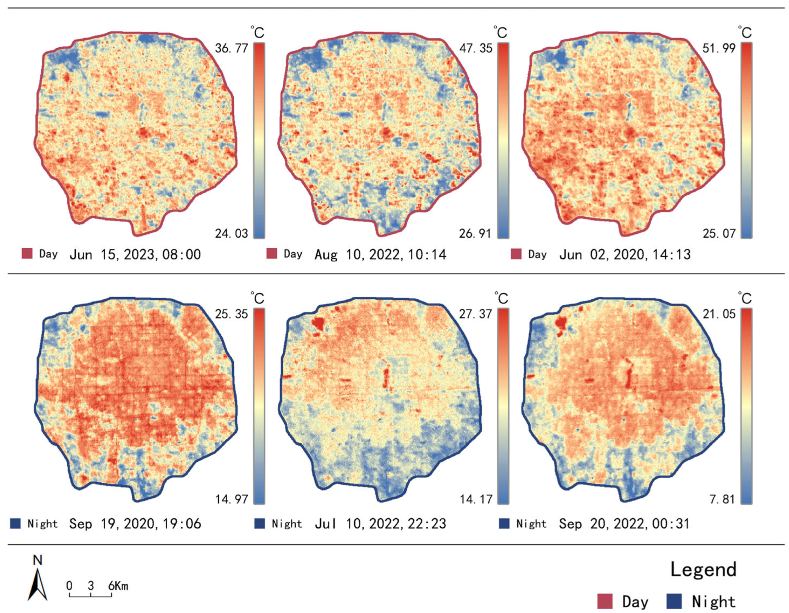
This study employs the ECOSTRESS Level-2 Land Surface Temperature and Emissivity (LST&E) product (NASA LP DAAC; https://lpdaac.usgs.gov/), derived using a physics-based Temperature Emissivity Separation (TES) algorithm. The product provides atmospherically corrected LST data from five thermal infrared bands at 70 m resolution, with validation showing global accuracy within ~1 K and an average uncertainty of 0.988 K. Each swath spans ~400 km, enabling high-resolution LST mapping. Given ECOSTRESS’s 3–5 day revisit cycle, LST measurements at different times were not acquired on the same day; thus, the results capture approximate diurnal patterns of urban influences on LST rather than exact same-day variations. To investigate UHI mitigation strategies, we focused on the four warmest months (June–September) of the year. Following the methodological framework of Chang et al. [3], Q. Wang et al. [22], and Y. Yan et al. [23], we selected six high-quality, cloud-free images acquired at approximately equal intervals. The image selection process followed a rigorous quality control protocol: (1) cloud cover ≤ 10% within the study area; (2) acquisition time falling within the warm season (June–September) to ensure consistency in seasonal thermal behavior; (3) temporal distribution spanning dawn, morning, afternoon, and evening to capture diurnal cycles; and (4) visual inspection to exclude images with residual cloud contamination or sensor anomalies. Although the selected images were not from the same day, they represent typical clear-sky conditions during the study period, minimizing potential bias from weather variability. The acquisition times were 20 September 2022, at 00:31; 15 June 2023, at 08:00; 10 August 2022, at 10:14; 2 June 2020, at 14:13; 19 September 2020, at 19:06; and 10 July 2022, at 22:23 (Figure 2).

2.3. Urban Characteristics

In this study, three datasets available on the Google Earth Engine (GEE) cloud platform—ESA WorldCover 2020, NOAA VIIRS DNB Monthly, and WorldPop—were used to obtain land cover, nighttime light, and population density data, respectively. Urban characteristics are inherently complex; therefore, to analyze their relationship with land surface temperature (LST), we quantified them into 18 metrics representing three dimensions: blue–green space, urban form, and population activities (

Table 1. Comprehensive information about the selected indicators.

Categories	Factors	Abbreviation	Description
Blue–green space	Normalized difference vegetation index	NDVI	The average NDVI in a block.
	Percentage of landscape area occupied by trees	TPLAND	The proportional abundance of tree land within a statistical unit.
	Percentage of landscape area occupied by crops	CPLAND	The proportional abundance of crop land within a statistical unit.
	Percentage of landscape area occupied by water	WPLAND	The proportional abundance of water areas within a statistical unit.
Urban form	Building height	BH	The average building height (m) in a statistical unit.
	Building density	BD	The proportional building footprints in a statistical unit.
	Sky view factor	SVF	The average SVF value in a statistical unit.
Population activities	Nighttime light	NTL	The mean value of NTL in a statistical unit for the detection of human activity.
	Population density	POP	Population counts in a statistical unit.

). The selection of these metrics was not arbitrary but was based on prior research findings and urban design considerations. Data mining and metric computation were performed primarily using Python 3.10 and ArcGIS Pro 3.3. Landscape pattern metrics and building-related factors were derived from land cover maps retrieved from the GEE platform. The imagery was imported into RStudio 4.4.20 for land use classification at a spatial resolution of 10 m, resulting in the identification of eight land cover classes: forest, shrubland, grassland, cropland, impervious surface, bare land, built-up land, and water bodies. Previous research [24] has shown that the relationships between percentage of landscape (PLAND), aggregation index (AI), landscape shape index (LSI), normalized difference vegetation index (NDVI), and LST are influenced by diurnal variations. Based on these findings, this study selected three landscape metrics—PLAND, AI, and LSI—for seven land cover types (excluding built-up land). The calculation formulas for these metrics are as follows:

$$PLAND={\displaystyle \frac{P_i}{A}}\times 100$$

(1)

$P_i$ is the proportion of landscape occupied by class i; $A$ is the total landscape area (m²).

All derived metrics were calculated at the community unit level to ensure spatial consistency. To validate the accuracy of the land cover classification, we performed a random sampling of 300 points across the study area and compared them with high-resolution Google Earth imagery. The overall accuracy reached 88.7%, with a Kappa coefficient of 0.85, indicating reliable classification results. Nighttime light and population density data were resampled to match the community unit boundaries using zonal statistics in ArcGIS Pro.

To mitigate the impact of multicollinearity on parameter estimation and inference, this study employed the variance inflation factor (VIF) to diagnose and screen candidate independent variables. We first calculated the VIF for each variable and iteratively removed those with excessively high VIF values (such as BVD and FAR). After each removal, the VIF of the remaining variables was recalculated. All retained variables ultimately had VIF values less than 5, indicating no significant multicollinearity in the dataset. The final set of variables included BH, SVF, NTL, BD, POP, NDVI, C_PLAND, T_PLAND, and W_PLAND. Using this filtered variable set, we proceeded with subsequent model fitting and SHAP (SHapley Additive exPlanation) interpretability analysis.

2.3.1. Blue–Green Space Variables

Blue–green space variables refer to areas covered by vegetation (green spaces) and water bodies (blue spaces), which represent natural elements within urban or landscape environments. They play a critical role in regulating urban thermal conditions and mitigating the UHI effect. Given the strong correlation between vegetation, water bodies, and LST, this study selected nine landscape indices with high correlations to analyze urban vegetation design. All these indices were derived from land cover maps. The normalized difference vegetation index (NDVI), calculated from remote sensing satellite data, is a widely used green space index in UHI studies and can be used to quantify the extent of green space in a two-dimensional spatial context [25]. The NDVI is calculated as follows:

$$NDVI={\displaystyle \frac{R_{NIR}-R_{RED}}{R_{NIR}+R_{RED}}}$$

(2)

$R_{NIR}$ is the reflectance in the near-infrared band; $R_{RED}$ stands for the reflectance in the red band.

2.3.2. Urban Form Variables

Seven urban form metrics were selected: building height (BH), building density (BD), built volume density (BVD), sky view factor (SVF), floor area ratio (FAR), bare land percentage (B_PLAND), and impervious surface percentage (I_PLAND). These indices reflect the spatial structure, density, and morphology of the built environment. The SVF, representing the proportion of sky visible from the ground, was calculated as follows:

$$SVF=1-\sum _{i=1}^n \mathrm{s}\mathrm{i}\mathrm{n}{\gamma }_i/n$$

(3)

${\gamma }_i$ stands for the elevation angle of the relief horizon, which can be calculated by computing the horizontal distance and elevation difference between the horizon and the vantage point; $n$ denotes the number of directions used to estimate $\gamma$. $SVF$s vary between 0 and 1. Values close to 1 represent open views from almost all angles, which is the case in exposed areas. In contrast, values close to 0 indicate views of the sky from deep urban canyons [26].

2.3.3. Population Activity Variables

Two indicators were used: population density (POP) and nighttime light intensity (NTL). NTL data from the VIIRS sensor provides a proxy for anthropogenic activity and energy use, while POP data from the WorldPop project offers high-resolution estimates of population distribution (100 m × 100 m).

2.4. LCZ Classification

The Local Climate Zone (LCZ) framework, originally proposed by Stewart and Ok, classifies urban areas into 17 standard types based on surface structure, cover, and human activity. However, the generic LCZ system may not fully capture the unique urban morphology of Chinese megacities such as Beijing, where neighborhood types are often shaped by regulatory detailed planning and historical preservation policies.

In contrast to previous LCZ mapping efforts in Beijing, such as the study by Zhou et al. [27], which used 300 × 300 m grid units and open data primarily for heat risk and population exposure assessment, the present study adopts a community-scale LCZ classification scheme following Chang et al. [3]. This approach integrates urban planning data and employs community units—the fundamental spatial units for urban management in China—as delineation boundaries to enhance planning applicability and support mechanistic analysis of the thermal environment.

We obtained building footprint data from the Beijing Municipal Planning and Natural Resources Commission, which includes building height and base area. For each community unit, we computed three key indicators: mean building height, mean building density, and percentage of green coverage. These values were compared against the thresholds defined in

Table 2. LCZ mapping scheme using planning data (‘–’ indicates that LCZ classes were mainly constrained by other metrics).

LCZ Classes	Built Types	Mean Building Height	Mean Building Density	Percentage of Green Coverage	Land Use Type
1	Compact high-rise	>30 m	>20%	–	–
2	Compact mid-rise	10–30 m	>20%	–	–
3	Compact low-rise	≤10 m	>20%	–	–
4	Open high-rise	>30 m	≤20%	–	–
5	Open mid-rise	10–30 m	≤20%	–	–
6	Open low-rise	≤10 m	≤20%	–	–
B	Scattered trees (e.g., urban park)	≤10 m	≤20%	>35%	Green land

to assign each community unit to one of the seven LCZ types.

To validate the LCZ classification, we conducted a visual comparison with high-resolution Google Earth imagery and performed a random sample check of 100 community units. The overall accuracy was 87%, with a Kappa coefficient of 0.83, confirming the reliability of the classification scheme. Although subclasses (e.g., LCZ 1A, 1B) were not included due to data granularity limitations, the seven-class system sufficiently captures major thermal contrasts within Beijing’s urban fabric, as supported by the observed LST variations in Section 3.2.

2.5. Research Framework

This study primarily employed the XGBoost regression model and (SHAP) to analyze the relationships between urban characteristic variables and LST.

2.5.1. XGBoost Regression Model

This study employed the XGBoost (eXtreme Gradient Boosting) algorithm to construct a regression model for analyzing the complex nonlinear relationships between urban characteristic variables and land surface temperature (LST). XGBoost is an efficient gradient boosting decision tree algorithm capable of effectively handling high-dimensional features and capturing interaction effects between variables [28,29].

This study implemented the XGBoost model using the XGBoost package in Python. We utilized 9 urban characteristic variables to predict LST and trained separate models for each of the six observation time points.

The dataset containing 9 urban characteristic variables was first preprocessed by uniformly replacing null values, spaces, and NaN values with 0, and converting all features to float type to ensure data consistency. The dataset was randomly split into training and testing sets in a 7:3 ratio using random sampling, with a random seed set to 42 to ensure reproducibility. Model training was carried out through the Python interface of XGBoost. To optimize model performance while preventing overfitting, the following hyperparameters were adopted: a learning rate of 0.01 and 200 boosting iterations. The predictive performance was assessed using the coefficient of determination (R²) and the root mean square error (RMSE). Across all six observation time points, the model achieved an average R² of 0.50 and an average RMSE of 0.76. These findings demonstrate that the XGBoost model provides consistent and effective predictive capability for LST throughout the diurnal cycle.

2.5.2. SHapley Additive exPlanation (SHAP)

This study employed SHAP, an interpretable machine learning approach [29,30]. Although machine learning models generally achieve high predictive accuracy, they are inherently opaque algorithms. In other words, such models often lack interpretability and are prone to overfitting due to sensitivity to the training data. By emphasizing interpretability and explanatory power, SHAP enhances the fairness of decision-making outcomes and can partially address the aforementioned issues [18]. SHAP primarily uses SHAP values to quantify the relative importance of independent variables on the dependent variable, calculated as the mean absolute SHAP value across all samples. In addition, SHAP can analyze the interaction effects between features and outcomes, i.e., the combined influence of two independent variables on the target. Specifically, it enables the quantification of the interaction effect of any feature pair (e.g., NDVI and FAR) for each sample. At present, SHAP is among the most widely used frameworks for interpreting machine learning results and has been extensively applied in recent studies [31].

XGBoost is a gradient boosting machine learning algorithm that builds an ensemble of decision trees to predict target variables. It is well-suited for evaluating the relative importance of multiple predictors and modeling nonlinear relationships [28,29]. In this study, the XGBoost model was trained using the 18 urban characteristic variables to predict LST at each of the six observation times.

3. Results

3.1. The LCZ Classification

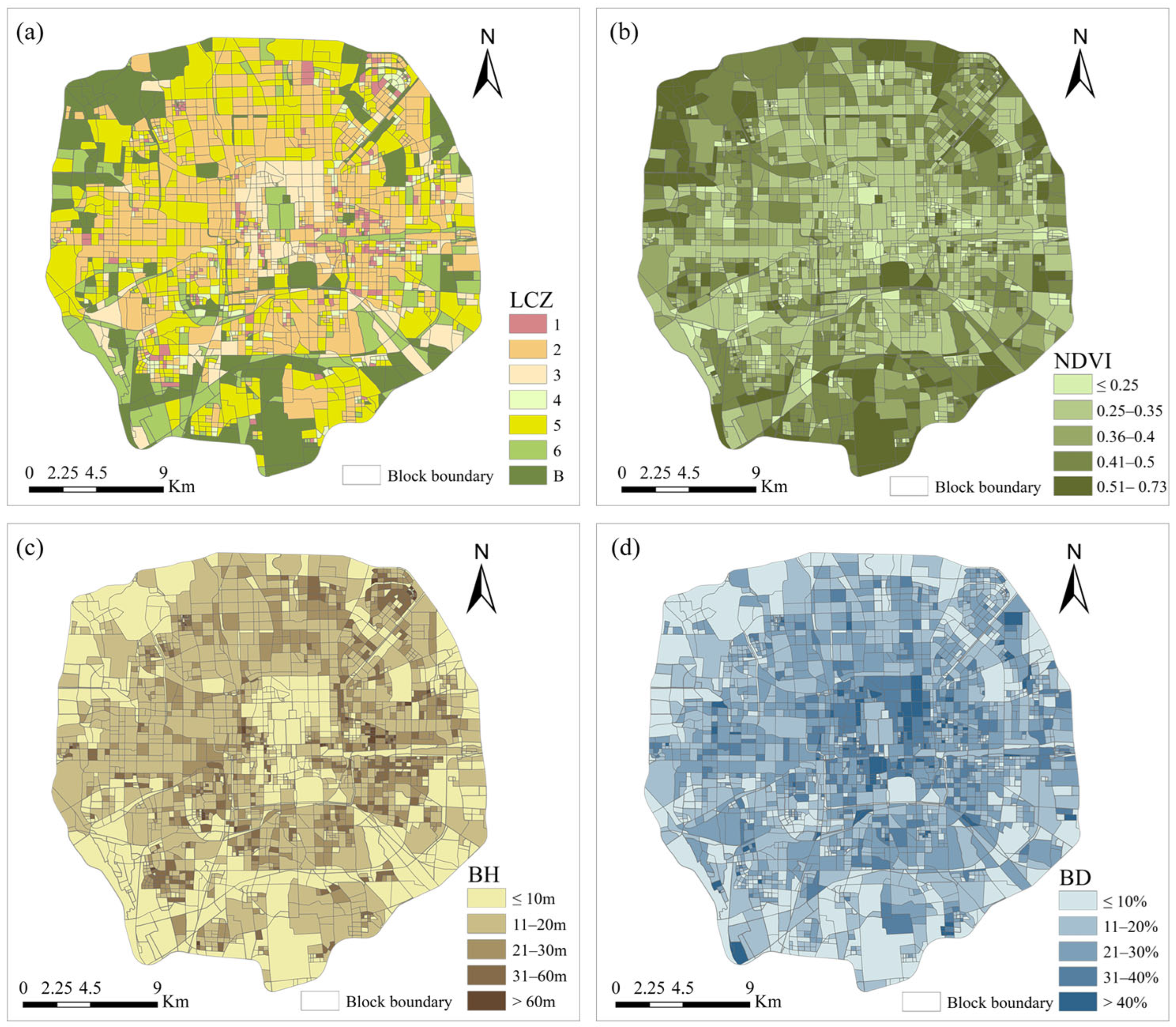
The study area was classified into seven LCZ types (Figure 3): compact high-rise (LCZ 1), compact mid-rise (LCZ 2), compact low-rise (LCZ 3), open high-rise (LCZ 4), open mid-rise (LCZ 5), open low-rise (LCZ 6), and scattered trees (LCZ B). LCZ 2 was predominantly located between the Second and Fourth Ring Roads, accounting for approximately half of the total LCZ area. This zone lies in the core of Beijing and has historically served as the city’s economic, commercial, and cultural hub. With the progression of urbanization, the municipal government adopted a relatively compact urban development model to optimize land use efficiency. Under this planning framework, mid-rise buildings became the preferred development form, meeting the growing residential demand while ensuring adequate transportation and public service infrastructure.

LCZ 3 was mainly distributed within the Second Ring Road, corresponding to the city’s historic core. To preserve clusters of ancient architectural heritage within the UNESCO World Heritage protection zone, building heights in this area are strictly regulated. This zone hosts a large concentration of historical structures, notably courtyard houses and alleyways dating back to the Ming and Qing dynasties.

LCZ 1 and LCZ 4 were sparsely distributed within the Fifth Ring Road, while LCZ 6 and LCZ B were concentrated on the urban periphery. As Beijing’s urbanization advanced, the original urban–rural fringe gradually transformed into newly developed urban and suburban districts. Open low-rise buildings typically appeared in these peripheral areas, which were formerly agricultural lands or relatively undeveloped zones. With the ongoing expansion of the urban edge, low-rise building development has become the dominant construction form in these locations.

3.2. Characteristics of Diurnal Variations in LST Across LCZ

This study analyzed and compared the spatial distribution of land surface temperature at six different times of the day based on the LCZ classification and LST data. The diurnal LST sequence followed the order of afternoon > morning > evening > dawn. This pattern reflects the daytime heat accumulation across all LCZs, followed by heat release during nighttime. These findings indicate that mitigation strategies targeting the urban heat island (UHI) effect should primarily focus on the daytime period when temperatures reach their peak.

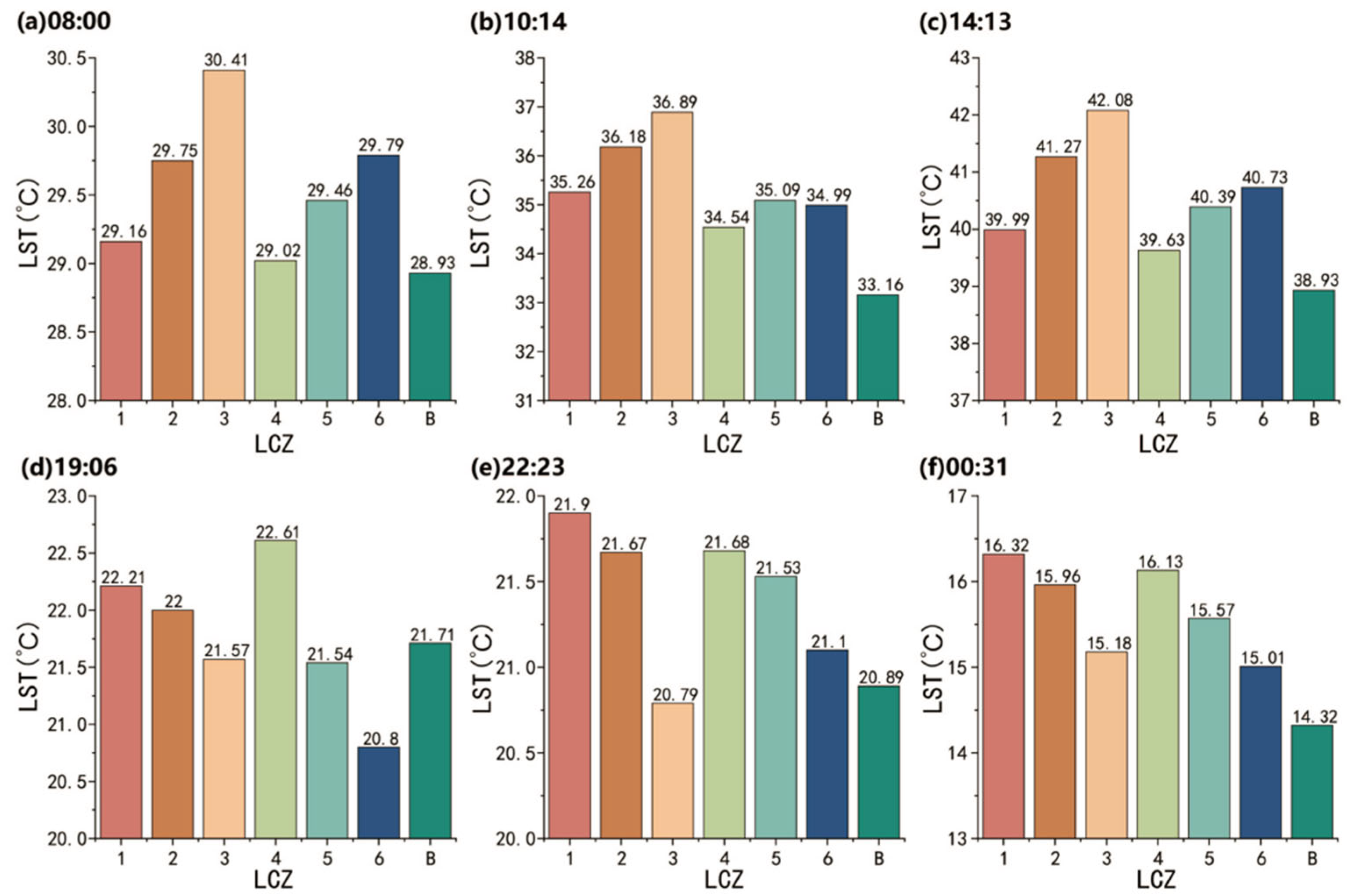
Figure 4 presents the statistical LST values for each LCZ at all observation times. During the daytime (08:00, 10:14, and 14:13), the seven LCZ types exhibited similar thermal patterns. LCZ 3 recorded the highest mean LST, followed by LCZ 2, LCZ 6, LCZ 5, LCZ 1, LCZ 4, and LCZ B. LCZ 3 had the highest mean LST because it typically comprises compact building clusters with limited vegetation, where artificial surfaces such as concrete and asphalt absorb and store more solar radiation. These materials generally have high heat capacity and thermal conductivity, causing them to rapidly accumulate heat during the day, resulting in elevated LST.

In contrast, LCZ B contains abundant green space and trees, which remove heat effectively through transpiration, thereby reducing surface temperatures. Vegetation provides significant cooling benefits, particularly during daytime, as evapotranspiration consumes a substantial amount of heat, leading to the lowest LST in these areas. As shown in

Table 3. Statistical analysis of LST for different LCZs at different observation times.

LCZ	1	2	3	4	5	6	B
Average temperature	27.47	27.81	27.82	27.27	27.26	27.07	26.32
Maximum temperature	39.99	41.27	42.08	39.63	40.39	40.73	38.93
Lowest temperature	16.32	15.96	15.18	16.13	15.57	15.01	14.32
Temperature difference	23.67	25.31	26.90	23.49	24.83	25.72	24.61

, LCZ 3 recorded the highest mean and maximum temperatures, LCZ B had the lowest mean and minimum temperatures, LCZ 3 exhibited the largest diurnal temperature range, and LCZ 1 displayed the smallest range. LCZ 1 consists mainly of high-rise buildings, which often use highly reflective materials (e.g., glass, aluminum) that absorb less heat during the day. Moreover, their tall structures limit direct sunlight exposure at ground level, slowing the rate of temperature increase.

The results also revealed temporal differences in LST between built-up and natural cover types. At 00:31, 08:00, 10:14, and 14:13, built-up surfaces consistently exhibited higher temperatures than natural cover types. However, at 19:06 and 22:23, the LST of some built-up areas fell below that of natural covers. This may be attributed to the rapid radiative cooling of hard surfaces in urban areas at night, resulting in lower temperatures, whereas vegetated surfaces—with higher moisture content and lower reflectivity—release heat more slowly through radiation, thereby maintaining relatively higher temperatures.

3.3. Results of the XGBoost Regression Model and SHAP

Based on previous studies, we selected variables that showed significant correlations with LST, including nine blue–green space variables, seven urban form variables, and two population activity variables. These variables were input into the XGBoost regression model, which was trained to obtain the optimal model. Finally, SHAP was used to calculate both the SHAP values and SHAP interaction values for the above variables [32], enabling the analysis of their relative importance and interaction effects on LST.

3.3.1. Relative Importance Ranking

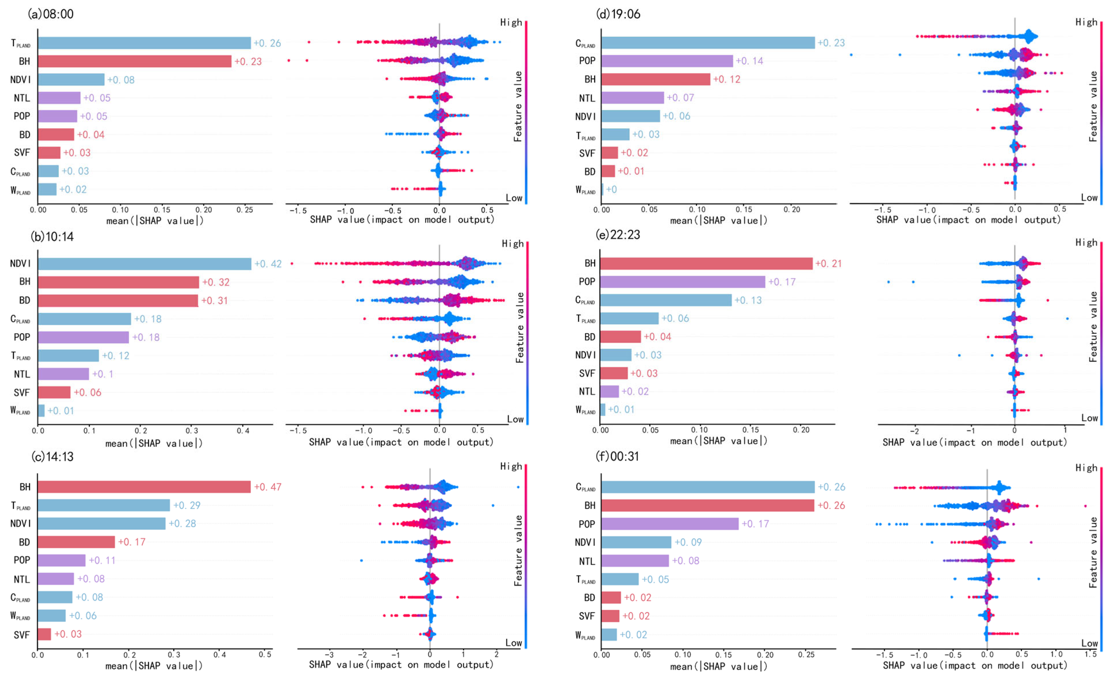
Figure 5 illustrates the SHAP-based interpretability results for the effects of urban characteristic variables on LST at six observation times, revealing the relative importance of different variables and their temporal variations. The left panel of the figure shows the ranking of variable importance, while the right panel uses a blue-to-red gradient to represent the range from the lowest to the highest feature values. For blue–green space variables, C_PLAND ranked first in relative importance at 00:31 and 19:06, T_PLAND ranked first at 08:00, and NDVI ranked first at 10:14. For urban form variables, BH ranked first in relative importance at 14:13 and 22:23. Across the six time points, BH appeared among the top three variables six times. For population activity variables, none ranked first at any time point; however, population density (POP) appeared among the top three variables three times.

Overall, the relative importance rankings can be broadly divided into two temporal patterns:

• Daytime (08:00–14:13), where T_PLAND, NDVI, and BH were the top three factors, although their order varied. These patterns suggest a strong association between vegetation, building height, and LST during daytime hours.
• Nighttime (19:06–00:31), where C_PLAND and BH were the top three factors. Notably, the importance of POP increased significantly at night, implying a potential link between human activities and nocturnal warming.

In addition, SVF and W_PLAND had relatively minor effects on LST.

3.3.2. Interaction Effects of Variables on LST

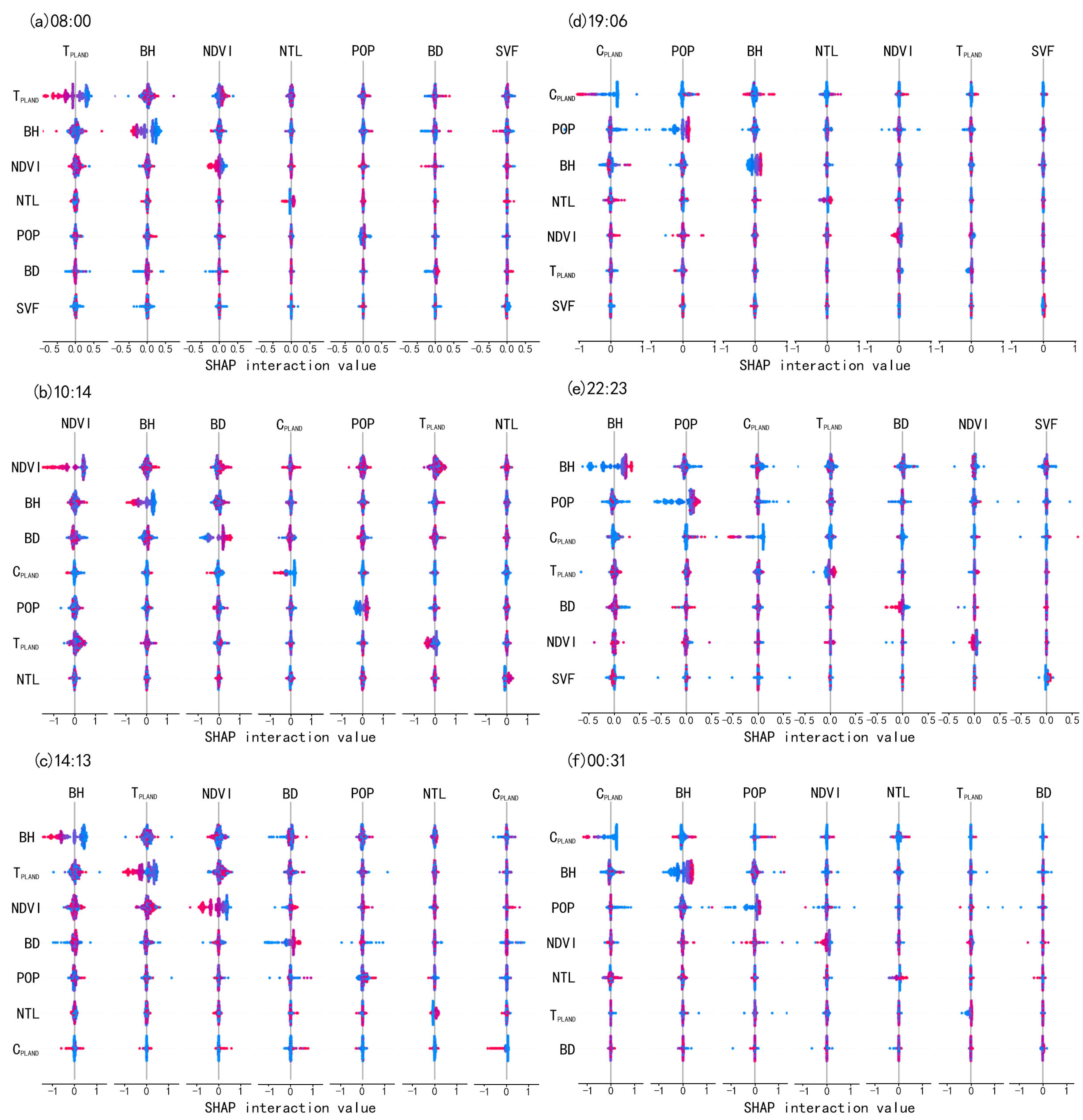
As shown in Figure 6, interaction effects exist between urban characteristic variables in relation to LST. The diagonal cells represent the effects of individual features, while the off-diagonal cells indicate the interaction effects between feature pairs. The results demonstrate strong interactions between T_PLAND–NDVI, C_PLAND–POP, T_PLAND–BH, and several other feature combinations.

During the daytime, notably strong interaction effects were observed for feature pairs such as T_PLAND–BH, NDVI–BD, and NDVI–T_PLAND. At night, strong interactions were found for C_PLAND–BH, C_PLAND–POP, and POP–BH.

These findings indicate that examining only the relationship between single variables and LST, as in many previous studies, is insufficient for fully understanding urban thermal dynamics. There is a pressing need to investigate the interaction effects of characteristic variables on LST, particularly those between (1) blue–green space variables, (2) blue–green space and urban form variables, and (3) blue–green space and population activity variables. These conclusions further underscore the necessity and novelty of this study.

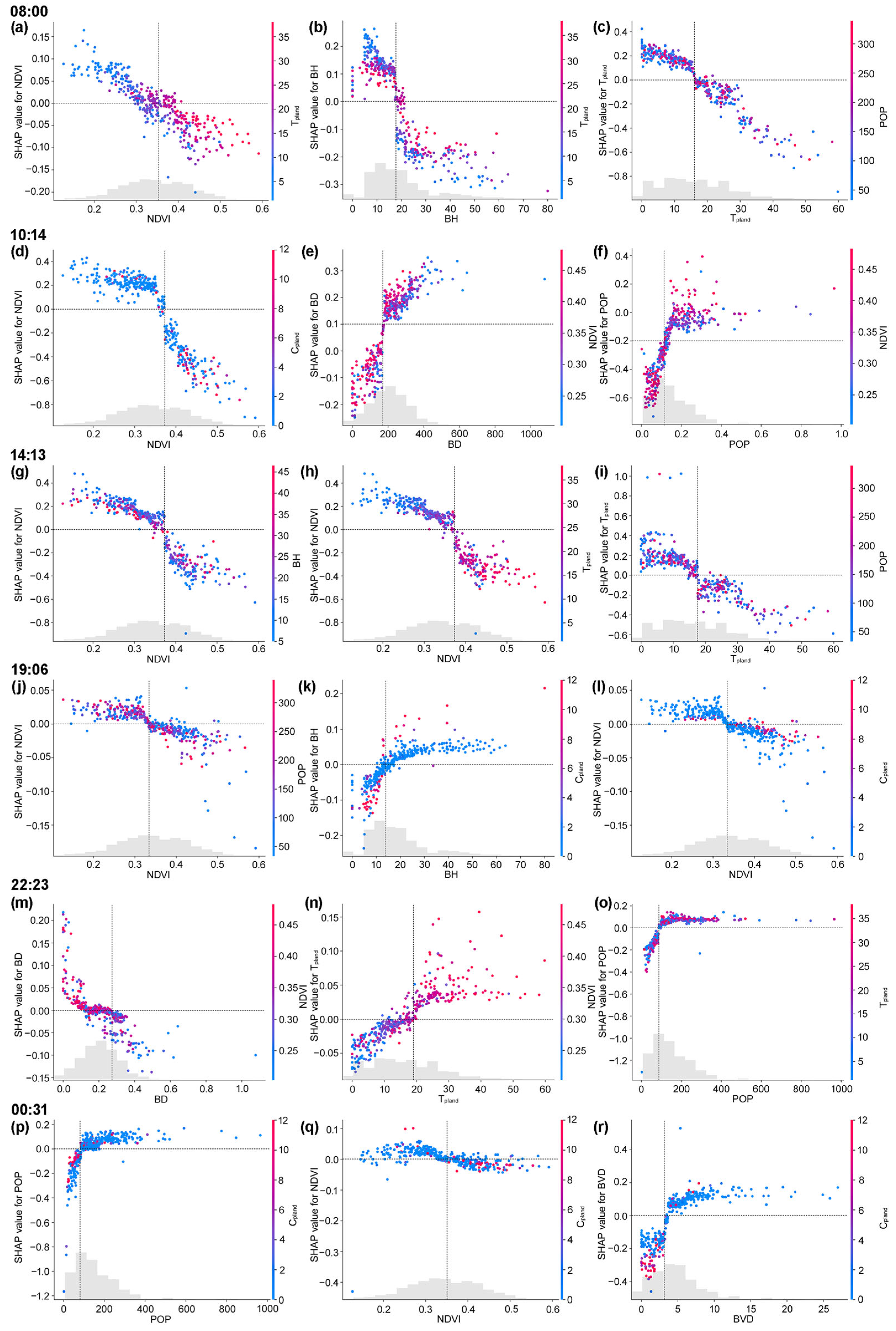
Based on the SHAP analysis of interaction effects between urban characteristics and LST and considering both the relative importance of individual variables and the strength of pairwise interactions, 18 representative feature pairs (e.g., NDVI and T_PLAND) were selected to examine their interaction effects on LST (Figure 7). It should be noted that these interaction plots are derived from machine learning model predictions and are intended to reveal potential patterns rather than establish causal relationships. In the plots, the SHAP interaction values are represented on the left Y-axis, the X-axis denotes the value of the first feature, and the right Y-axis represents the value of the second feature, with colors ranging from blue (low) to red (high). The feature pairs were classified into three categories: blue–green space and blue–green space, blue–green space and urban form, and blue–green space and population activity. For each category, three representative pairs were selected for the six observation times to investigate their interaction effects on LST.

(1) Blue–green space and blue–green space pairs: As shown in Figure 7a, at 08:00, when NDVI exceeded 0.36 and TPLAND exceeded 20%, LST decreased. A similar effect was observed at 14:13 when NDVI exceeded 0.37 and TPLAND exceeded 20% (Figure 7h). However, at 22:23, when NDVI exceeded 0.35 and TPLAND exceeded 20%, LST increased (Figure 7n). This is because vegetation cools the surface during the day through evapotranspiration and reflection, but, at night, when transpiration weakens, vegetation tends to retain heat, leading to higher LST in vegetated areas, thus confirming the inference in Section 3.2. In addition, at 10:14, when NDVI exceeded 0.37 and C_PLAND was below 8%, LST decreased (Figure 7d). A similar pattern was observed at 19:06 when NDVI exceeded 0.34 and C_PLAND was below 4% (Figure 7k). Since high NDVI generally indicates healthy vegetation, these results suggest that, even with a low proportion of cropland, healthy vegetation can effectively absorb heat and cool the surface through evapotranspiration. Therefore, urban planning should prioritize the management of vegetation health and quality rather than only increasing green coverage.

(2) Blue–green space and urban form pairs: At 10:14, when BD was below 0.18 and NDVI exceeded 0.35, LST decreased (Figure 7e). However, at 22:23, when BD was below 0.24 and NDVI exceeded 0.35, LST increased (Figure 7m). This diurnal reversal can be explained by contrasting the physical processes governing surface energy balance between day and night. During the daytime, low BD implies fewer buildings and more exposed surfaces, allowing greater penetration of solar radiation. Vegetation (high NDVI) provides shading and facilitates evapotranspiration, both of which reduce sensible heat flux and lower LST. The combined effect of reduced heat storage from built structures and active cooling from vegetation leads to a net cooling effect. However, at nighttime, the absence of solar radiation shifts the dominant process to longwave radiative cooling and convective heat loss. In low-BD areas, the lack of building mass results in lower thermal inertia, allowing surfaces to cool rapidly. However, vegetation canopies trap outgoing longwave radiation and impede ventilation near the surface, thereby reducing the rate of radiative cooling and convective heat dissipation. Additionally, vegetation itself releases stored moisture and heat slowly through nighttime evapotranspiration, further slowing the cooling process. Consequently, even with low building density, the presence of dense vegetation (high NDVI) can lead to higher nocturnal LST compared with more open or paved surfaces that cool more efficiently. These findings underscore the need for urban planning strategies that account for the diurnal shift in thermal regulation mechanisms. For instance, in low-BD areas with high vegetation cover, incorporating open sky exposure and enhancing nighttime ventilation through strategic landscape design could help mitigate nocturnal heat retention.

(3) Blue–green space and population activity pairs: At 08:00, when TPLAND exceeded 16% and POP was below 250 persons/ha, LST decreased (Figure 7c). A similar effect occurred at 14:13 when T_PLAND exceeded 17% and POP was below 200 persons/ha (Figure 7i). However, at 22:23, when TPLAND exceeded 15% and POP exceeded 180 persons/ha, LST increased (Figure 7o). During the day, trees significantly reduce LST through transpiration, shading, and reflection. In low-POP areas, reduced building mass limits heat absorption and storage, enhancing the cooling effect of vegetation. However, at night, accumulated heat from buildings and impervious surfaces (e.g., streets, rooftops) is gradually released. Higher POP typically corresponds to greater building density, traffic, and human activity, which contribute to additional heat release into the environment. Consequently, even in areas with high T_PLAND, the release of heat from built structures can lead to LST increases. Therefore, in high-POP areas such as city centers, temperature management strategies should include rooftop greening, permeable pavements, and high-reflectance building materials to mitigate nighttime warming.

4. Discussion

4.1. The Impacts of LCZ Spatial Patterns on Thermal Environment

Considering the specific urban context of Beijing, a typical megacity in China, this study adopted a simple and efficient LCZ delineation method: the community-based LCZ scheme. The results indicate that the spatial patterns of LST in urban areas vary across different times of the day. Such variation is primarily attributed to the capacity of buildings and other impervious surfaces to store more radiative energy during the day, leading to a gradual decline in LST as the stored heat is released [5,33]. Compact building zones heat up more rapidly than open building zones, and their LST is generally higher. This is because open-form buildings allow better ventilation, which facilitates convective heat transfer from the ground and building surfaces into the atmosphere [34].

Furthermore, this study revealed that, during the daytime, the LST in compact building zones is significantly higher than in open building zones; however, at night, the LST of the two tends to converge. At night, when solar radiation ceases, heat stored at the surface dissipates via radiative cooling [3]. Due to their higher building density, compact building zones accumulate more heat during the day, which is released more rapidly at night [5]. In contrast, open building zones, with fewer buildings and more green and open spaces, tend to release heat more gradually.

Additionally, during the daytime, low-rise LCZs within compact building zones exhibit significantly higher LST than high-rise LCZs, whereas, in open building zones, high-rise LCZs have higher LST than low-rise LCZs. This difference can be explained by the fact that high-rise buildings generally cast more shade than low-rise structures, thereby reducing the amount of solar radiation reaching the ground [3]. The pronounced urban canyon effect in high-rise areas also contributes to lower LST in compact building zones [26]. Consequently, previous studies have recommended increasing building height to provide greater shading [35,36,37], although this recommendation applies mainly to compact building zones. Overall, these findings enhance our understanding of how complex urban landscapes influence the spatial heterogeneity of LST in metropolitan environments.

4.2. Spatial Effects of Urban Features on LST

LST is influenced by a wide range of intra-urban factors and thus requires a multidimensional perspective for comprehensive assessment. This study primarily examined the relative importance and interaction effects of urban characteristics on LST, providing empirical insights and recommendations to support urban surface heat balance and regional sustainable development. Previous studies have consistently demonstrated that LST is highly sensitive to human activities and urban morphology. Building on this foundation, our work incorporates diverse vegetation landscape pattern characteristics and explores the spatial effects of urban characteristics on LST from three perspectives: blue–green space, urban form, and human activity.

The results indicate that C_PLAND, T_PLAND, NDVI, and BH are the key determinants of LST. C_PLAND, T_PLAND, and NDVI exhibit strong negative correlations with LST, particularly during the daytime. Numerous studies have confirmed that the cooling effect of blue–green spaces is primarily attributed to plant transpiration, canopy shading, and the high specific heat capacity of water bodies [38,39,40,41]. Therefore, where spatially and economically feasible in central urban areas and zones with high population density, it is recommended to strengthen green infrastructure development by increasing vegetation coverage through the establishment of urban parks, green belts, and rooftop gardens.

BH shows a negative correlation with LST during the day but a positive correlation at night. In daytime conditions, taller buildings typically provide more shading, thereby reducing direct solar radiation on the ground and lowering surface temperatures in their vicinity [3], especially in densely built-up areas [41]. Moreover, high-rise buildings possess greater heat capacity, enabling them to absorb more solar radiation and thermal energy during the day. Consequently, at night, as the stored heat is released, areas with higher building density exhibit elevated temperatures compared with areas with lower building density [35]. In residential neighborhoods and other areas with intensive nighttime activities, it is advisable to evaluate the potential benefits of regulating high-rise building density and exploring the integration of mid- and low-rise structures or ventilation corridors to facilitate heat dissipation while balancing other urban development goals.

4.3. Strategies to Improve the Beijing Thermal Environment in Future Development

The urban heat island (UHI) effect is an anthropogenic phenomenon that has emerged alongside urbanization. This implies that adaptation strategies within urban planning can alter the urban energy balance and improve thermal environments. Considering that extreme temperatures occur more frequently in summer, this study focuses on developing mitigation strategies for UHI during this critical season, though their efficacy may vary under different climatic and urban contexts.

4.3.1. Optimizing Urban Form

The results of this study indicate that compact building zones—particularly compact high-rise areas (LCZ 1)—exhibit significantly higher daytime LST than open high-rise areas (LCZ 4). Therefore, future urban planning should prioritize the development of open high-rise configurations and reasonably control building density in compact areas. Increasing open spaces may enhance heat dissipation and help alleviate the UHI effect, though the specific design and scale of such interventions should be tailored to local morphological and climatic conditions.

4.3.2. Expanding Blue–Green Infrastructure

The findings of this study show that large vegetated patches, especially in urban cores, can substantially reduce daytime LST. Accordingly, future planning should emphasize integrating large green areas with public spaces such as plazas, commercial districts, and residential neighborhoods to create multifunctional ecosystems [42]. However, the cooling efficacy of blue–green infrastructure is influenced by local climate, vegetation type, irrigation practices, and maintenance levels. Moreover, vegetation quality (e.g., NDVI) in this study appears more critical than mere coverage percentage. Healthy vegetation can effectively absorb heat and lower LST even in areas with relatively low coverage. Urban planners should thus consider prioritizing vegetation health maintenance and enhancement, rather than focusing solely on increasing green area extent.

To effectively expand blue–green infrastructure, urban planning requires not only technical design but also supportive policy instruments. First, regulatory instruments such as zoning codes and land use regulations can mandate minimum green coverage ratios, protect existing water bodies, and prevent further loss of ecological land. Second, economic instruments, including subsidies, tax incentives, and green financing schemes, can encourage private developers and communities to invest in rooftop gardens, permeable pavements, and urban wetlands. Third, planning and strategic instruments such as long-term ecological masterplans and integrated water–green infrastructure strategies can provide systematic guidance for incorporating blue–green elements into new developments and urban renewal projects. Finally, collaborative instruments involving public–private partnerships, community participation, and environmental stewardship programs are essential to ensure sustainable maintenance and enhance public awareness. In the context of Beijing, combining top-down regulations (e.g., municipal green quotas) with bottom-up initiatives (e.g., community park co-management) may create synergies that maximize both ecological and social benefits. By adopting a comprehensive mix of regulatory, economic, and participatory policy tools, cities can better institutionalize the role of blue–green infrastructure in mitigating the urban heat island effect and fostering climate-resilient urban environments.

4.3.3. Regulating Population Density and Human Activities

POP and NTL are key determinants of LST, particularly at night. High-population-density areas are often associated with increased energy consumption, vehicle emissions, and anthropogenic heat release from buildings, all of which contribute to elevated LST. To address this, urban planners could consider implementing strategies to mitigate heat emissions in densely populated zones, such as promoting energy-efficient buildings, encouraging public transportation, and enforcing green building standards. Additionally, incorporating rooftop greening and permeable pavements in high-density areas can enhance nighttime heat dissipation. The feasibility and effectiveness of these measures depend on local socio-economic conditions, governance structures, and existing infrastructure.

4.3.4. Balancing Daytime Cooling and Nighttime Heat Release

This study reveals that factors influencing LST differ between day and night, necessitating a balanced approach to daytime cooling and nighttime heat release. For example, while increasing BH can provide shading during the day, it may also lead to elevated nighttime temperatures. To mitigate this trade-off, planners could employ low-heat-capacity materials in high-rise construction or design buildings with enhanced nighttime ventilation to facilitate heat release. Further empirical research is needed to evaluate the real-world performance, cost-effectiveness, and scalability of these strategies.

4.4. Limitations of This Study and Future Work

Our analysis has several limitations and uncertainties that should be considered when interpreting the results and their generalizability.

First, this study relied solely on satellite-derived land surface temperature (LST). While LST is a valuable indicator of surface thermal patterns, it differs from air temperature (T~a~), which is more directly related to human thermal comfort and the canopy layer urban heat island (UHI) effect. The relationship between LST and T~a~ can be complex and varies with surface properties and meteorological conditions. The absence of concurrent air temperature measurements limits our ability to fully assess the human-scale heat island dynamics. Future studies should integrate satellite LST with in situ air temperature sensors or mobile measurements to provide a more comprehensive understanding of urban thermal environments.

Second, this study focuses solely on Beijing and its specific humid continental climate. Therefore, the findings and resulting policy recommendations presented in this study are most directly applicable to cities with similar climatic conditions and urban morphological characteristics (e.g., high-density, rapid urbanization). The transferability of these findings to cities in drastically different climatic zones (e.g., arid, tropical) or with distinct urban forms (e.g., highly sprawling cities) may be limited. Future research should extend the analysis to multiple cities across different climatic zones to further validate and generalize the relationships between urban characteristics and LST.

Third, while this study controlled for a wide range of urban morphological and cover characteristics, other potential confounding factors were not explicitly accounted for. Socio-economic heterogeneity (e.g., income levels, energy consumption patterns not captured by NTL or POP), urban management policies (e.g., differential irrigation practices in green spaces, waste heat management), and subtle remote sensing anomalies (e.g., undetected sub-pixel clouds, seasonal variations in vegetation phenology beyond NDVI) could influence the observed LST patterns. Although the machine learning approach can capture complex associations, causal inferences should be made with caution.

Furthermore, while the SHAP analysis revealed compelling interaction patterns between urban variables and LST, it is important to note that these relationships are based on correlational data and model outputs. The mechanisms suggested here should be further validated through controlled experiments or physical modeling before definitive causal conclusions can be drawn.

Regarding LCZ classification, we adopted a community-based LCZ mapping scheme and did not incorporate LCZ subclasses. Future work could refine the LCZ classification to better capture thermal differences and diurnal variations among urban landscape units.

Moreover, subsequent research could further explore the links between built environments and LST across the Beijing–Tianjin–Hebei region or investigate the mechanisms of LST variation in megacities located in different building–climate zones, thereby strengthening the evidence for the importance of urban characteristic variables in regulating LST. In addition, future studies should take into account the potential impacts of ongoing climate change in Beijing on urban thermal heterogeneity. In recent decades, Beijing has experienced a notable warming trend, with more frequent and intense heatwaves as well as shifts in precipitation patterns. These climatic changes may exacerbate intra-urban temperature contrasts by amplifying the cooling demand of densely built-up areas while simultaneously altering the performance of blue–green infrastructure. For instance, prolonged droughts could weaken the evapotranspiration capacity of urban vegetation, whereas extreme rainfall events may temporarily enhance surface cooling but also increase surface runoff and reduce infiltration efficiency. Therefore, future research should integrate climate change projections and long-term monitoring data to assess how evolving climatic conditions interact with urban morphology and land cover. This approach would provide more robust and forward-looking evidence for developing climate-resilient strategies to mitigate the urban heat island effect in Beijing and similar megacities.

5. Conclusions

This study employed LST data from the ECOSTRESS sensor onboard the International Space Station to investigate the diurnal variation in the urban thermal environment in Beijing, China, and examine the influence of urban characteristics on LST. A community-based LCZ classification scheme was adopted to facilitate the analysis of thermal effects in spatially heterogeneous urban landscapes. We then assessed the thermal behavior of different LCZs at multiple daytime and nighttime periods and evaluated both the relative importance and interaction effects of various urban characteristic variables on LST using XGBoost and SHAP analysis. While similar integrative approaches have begun to emerge in recent urban climate literature, this study contributes to the growing body of evidence by applying this framework to a high-density Asian megacity with a humid continental climate.

The main findings of this study are as follows:

• Significant differences in LST across LCZ types: Compact building zones (LCZ 1, LCZ 2, and LCZ 3) exhibited higher daytime LST compared with open building zones (LCZ 4, LCZ 5, and LCZ 6), while nighttime temperature differences between the two were notably smaller. The scattered trees zone (LCZ B) provided strong daytime cooling through evapotranspiration, but its effect diminished at night.
• Diurnal variation in the importance of blue–green infrastructure, urban morphology, and human activity variables: Blue–green space variables had the strongest influence on daytime LST, with NDVI ranking first in relative importance at 10:14 and T_PLAND ranking first at 08:00, indicating that vegetation significantly reduced daytime LST through evapotranspiration and shading. Urban morphology variables were more influential at night, with BH ranking first at both 14:13 and 22:23, suggesting that tall buildings affect LST differently through shading in the daytime and heat storage at night. Human activity variables contributed significantly to nighttime LST increases, with POP ranking second and third at 19:06 and 00:31, respectively, implying that population-related heat emissions from energy use and traffic substantially elevate nocturnal LST.
• Strong interaction effects between variable types, varying between day and night: During the day, blue–green space and urban morphology variables interacted significantly: when NDVI exceeded 0.35 and BD was below 0.18, LST decreased markedly, indicating that low BD combined with high NDVI effectively reduced surface temperatures. However, at night, when NDVI exceeded 0.35 and BD was below 0.24, LST increased, suggesting that heat release from buildings and the thermal retention effect of vegetation jointly contributed to higher nocturnal temperatures. Interactions between blue–green space and human activity variables also displayed diurnal variation: during the day, high-TPLAND and lowPOP areas showed substantial cooling, while at night, high T_PLAND combined with high POP was associated with elevated LST. Interactions between urban morphology and human activity variables were particularly evident at night, as heat stored by tall buildings during the day and anthropogenic heat from nighttime activities jointly intensified nocturnal LST.

Overall, our results demonstrate that combining ECOSTRESS LST data with machine learning can substantially improve understanding of how blue–green infrastructure and other urban characteristics influence LST dynamics across the diurnal cycle. By analyzing multi-temporal data within a 24-h period, this study reveals the temporal shifts in variable importance and their nonlinear effects, addressing limitations of previous research that relied on single time points, single factors, or linear assumptions. The findings provide context-specific insights for urban planning and UHI mitigation strategies in cities with similar climatic and morphological characteristics. However, the generalizability of these results to other megacities—particularly those in different climatic zones or with distinct urban forms—requires further validation through multi-city comparative studies. Future research should expand this integrative approach to diverse urban settings to develop more universally applicable and resilient strategies for sustainable urban thermal management.

References

1. Kovats, R.S.; Campbell-Lendrum, D.; Matthies, F. Climate Change and Human Health: Estimating Avoidable Deaths and Disease. Risk Anal. 2005, 25, 1409–1418. [Google Scholar] [CrossRef] [PubMed]
2. Bečić, D.; Gašparović, M. Urban Heat Islands and Land-Use Patterns in Zagreb: A Composite Analysis Using Remote Sensing and Spatial Statistics. Land 2025, 14, 1470. [Google Scholar] [CrossRef]
3. Chang, Y.; Xiao, J.; Li, X.; Middel, A.; Zhang, Y.; Gu, Z.; Wu, Y.; He, S. Exploring Diurnal Thermal Variations in Urban Local Climate Zones with ECOSTRESS Land Surface Temperature Data. Remote Sens. Environ. 2021, 263, 112544. [Google Scholar] [CrossRef]
4. Xu, J.; Xuan, L.; Li, C.; Wu, T.; Wang, Y.; Wang, Y.; Wang, X.; Wang, Y. Effect of Landscape Architectural Characteristics on LST in Different Zones of Zhengzhou City, China. Land 2025, 14, 1581. [Google Scholar] [CrossRef]
5. Zhao, L.; Lee, X.; Smith, R.B.; Oleson, K. Strong Contributions of Local Background Climate to Urban Heat Islands. Nature 2014, 511, 216–219. [Google Scholar] [CrossRef] [PubMed]
6. Mishra, A.; Arya, D.S. Assessment of Land-Use Land-Cover Dynamics and Urban Heat Island Effect of Dehradun City, North India: A Remote Sensing Approach. Environ. Dev. Sustain. 2024, 26, 22421–22447. [Google Scholar] [CrossRef]
7. Naikoo, M.W.; Rihan, M.; Ishtiaque, M.; Shahfahad. Analyses of Land Use Land Cover (LULC) Change and Built-up Expansion in the Suburb of a Metropolitan City: Spatio-Temporal Analysis of Delhi NCR Using Landsat Datasets. J. Urban Manag. 2020, 9, 347–359. [Google Scholar] [CrossRef]
8. Naim, M.N.H.; Kafy, A.A. Assessment of Urban Thermal Field Variance Index and Defining the Relationship between Land Cover and Surface Temperature in Chattogram City: A Remote Sensing and Statistical Approach. Environ. Chall. 2021, 4, 100107. [Google Scholar] [CrossRef]
9. Stewart, I.D.; Oke, T.R. Local Climate Zones for Urban Temperature Studies. Bull. Am. Meteorol. Soc. 2012, 93, 1879–1900. [Google Scholar] [CrossRef]
10. Cai, M.; Ren, C.; Xu, Y.; Dai, W.; Wang, X.M. Local Climate Zone Study for Sustainable Megacities Development by Using Improved WUDAPT Methodology—A Case Study in Guangzhou. Procedia Environ. Sci. 2016, 36, 82–89. [Google Scholar] [CrossRef]
11. He, S.; Zhang, Y.; Gu, Z.; Su, J. Local Climate Zone Classification with Different Source Data in Xi’an, China. Indoor Built Environ. 2019, 28, 1190–1199. [Google Scholar] [CrossRef]
12. Peiró, M.N.; Sánchez, C.S.G.; González, F.N. Source Area Definition for Local Climate Zones Studies. A Systematic Review. Build. Environ. 2019, 148, 258–285. [Google Scholar] [CrossRef]
13. Jenerette, G.D.; Harlan, S.L.; Buyantuev, A.; Stefanov, W.L.; Declet-Barreto, J.; Ruddell, B.L.; Myint, S.W.; Kaplan, S.; Li, X. Micro-Scale Urban Surface Temperatures Are Related to Land-Cover Features and Residential Heat Related Health Impacts in Phoenix, AZ USA. Landsc. Ecol. 2016, 31, 745–760. [Google Scholar] [CrossRef]
14. Luo, P.; Yu, B.; Li, P.; Liang, P.; Liang, Y.; Yang, L. How 2D and 3D Built Environments Impact Urban Surface Temperature under Extreme Heat: A Study in Chengdu, China. Build. Environ. 2023, 231, 110035. [Google Scholar] [CrossRef]
15. Greene, C.S.; Millward, A.A. Getting Closure: The Role of Urban Forest Canopy Density in Moderating Summer Surface Temperatures in a Large City. Urban Ecosyst. 2017, 20, 141–156. [Google Scholar] [CrossRef]
16. Sun, Y.; Gao, C.; Li, J.; Li, W.; Ma, R. Examining Urban Thermal Environment Dynamics and Relations to Biophysical Composition and Configuration and Socio-Economic Factors: A Case Study of the Shanghai Metropolitan Region. Sustain. Cities Soc. 2018, 40, 284–295. [Google Scholar] [CrossRef]
17. Chen, X.; Wang, Z.; Yang, H.; Ford, A.C.; Dawson, R.J. Impacts of Urban Densification and Vertical Growth on Urban Heat Environment: A Case Study in the 4th Ring Road Area, Zhengzhou, China. J. Clean. Prod. 2023, 410, 137247. [Google Scholar] [CrossRef]
18. Wei, X.; Guan, F.; Zhang, X.; Van de Weghe, N.; Huang, H. Integrating Planar and Vertical Environmental Features for Modelling Land Surface Temperature Based on Street View Images and Land Cover Data. Build. Environ. 2023, 235, 110231. [Google Scholar] [CrossRef]
19. Xu, H.; Li, C.; Hu, Y.; Li, S.; Kong, R.; Zhang, Z. Quantifying the Effects of 2D/3D Urban Landscape Patterns on Land Surface Temperature: A Perspective from Cities of Different Sizes. Build. Environ. 2023, 233, 110085. [Google Scholar] [CrossRef]
20. Peel, M.C.; Finlayson, B.L.; McMahon, T.A. Updated World Map of the Köppen-Geiger Climate Classification. Hydrol. Earth Syst. Sci. 2007, 11, 1633–1644. [Google Scholar] [CrossRef]
21. Oke, T.R.; Mills, G.; Christen, A.; Voogt, J.A. Urban Climates; Cambridge University Press: Cambridge, UK, 2017; ISBN 978-0-521-84950-0. [Google Scholar]
22. Wang, Q.; Wang, X.; Meng, Y.; Zhou, Y.; Wang, H. Exploring the Impact of Urban Features on the Spatial Variation of Land Surface Temperature within the Diurnal Cycle. Sustain. Cities Soc. 2023, 91, 104432. [Google Scholar] [CrossRef]
23. Yan, Y.; Jian, W.; Wang, B.; Liu, Z. Multi-Scale Effects of LCZ and Urban Green Infrastructure on Diurnal Land Surface Temperature Dynamics. Sustain. Cities Soc. 2024, 117, 105945. [Google Scholar] [CrossRef]
24. Liu, W.; Zhang, L.; Hu, X.; Meng, Q.; Qian, J.; Gao, J.; Li, T. Nonlinear Effects of Urban Multidimensional Characteristics on Daytime and Nighttime Land Surface Temperature in Highly Urbanized Regions: A Case Study in Beijing, China. Int. J. Appl. Earth Obs. Geoinf. 2024, 132, 104067. [Google Scholar] [CrossRef]
25. Yang, J.; Dong, J.; Xiao, X.; Dai, J.; Wu, C.; Xia, J.; Zhao, G.; Zhao, M.; Li, Z.; Zhang, Y.; et al. Divergent Shifts in Peak Photosynthesis Timing of Temperate and Alpine Grasslands in China. Remote Sens. Environ. 2019, 233, 111395. [Google Scholar] [CrossRef]
26. Li, J.; Song, C.; Cao, L.; Zhu, F.; Meng, X.; Wu, J. Impacts of Landscape Structure on Surface Urban Heat Islands: A Case Study of Shanghai, China. Remote Sens. Environ. 2011, 115, 3249–3263. [Google Scholar] [CrossRef]
27. Zhou, Y.; Zhang, G.; Jiang, L.; Chen, X.; Xie, T.; Wei, Y.; Xu, L.; Pan, Z.; An, P.; Lun, F. Mapping Local Climate Zones and Their Associated Heat Risk Issues in Beijing: Based on Open Data. Sustain. Cities Soc. 2021, 74, 103174. [Google Scholar] [CrossRef]
28. Chen, T.; Guestrin, C. XGBoost: A Scalable Tree Boosting System. In Proceedings of the 22nd ACM SIGKDD International Conference on Knowledge Discovery and Data Mining, San Francisco, CA, USA, 13–17 August 2016; pp. 785–794. [Google Scholar]
29. Lan, H.; Hou, H.; Gou, Z. A Machine Learning Led Investigation to Understand Individual Difference and the Human-Environment Interactive Effect on Classroom Thermal Comfort. Build. Environ. 2023, 236, 110259. [Google Scholar] [CrossRef]
30. Hou, L.; Dai, Q.; Song, C.; Liu, B.; Guo, F.; Dai, T.; Li, L.; Liu, B.; Bi, X.; Zhang, Y.; et al. Supplementary Materials for Revealing Drivers of Haze Pollution by Explainable Machine Learning. Environ. Sci. Technol. Lett. 2022, 9, 112–119. [Google Scholar] [CrossRef]
31. Zheng, G.; Zhang, Y.; Yue, X.; Li, K. Interpretable Prediction of Thermal Sensation for Elderly People Based on Data Sampling, Machine Learning and SHapley Additive exPlanations (SHAP). Build. Environ. 2023, 242, 110602. [Google Scholar] [CrossRef]
32. Doan, Q.C.; Ma, J.; Chen, S.; Zhang, X. Nonlinear and Threshold Effects of the Built Environment, Road Vehicles and Air Pollution on Urban Vitality. Landsc. Urban Plan. 2025, 253, 105204. [Google Scholar] [CrossRef]
33. Li, X.; Zhou, Y.; Asrar, G.R.; Imhoff, M.; Li, X. The Surface Urban Heat Island Response to Urban Expansion: A Panel Analysis for the Conterminous United States. Sci. Total Environ. 2017, 605–606, 426–435. [Google Scholar] [CrossRef]
34. Zhang, J.; Li, Z.; Wei, Y.; Hu, D. The Impact of the Building Morphology on Microclimate and Thermal Comfort-a Case Study in Beijing. Build. Environ. 2022, 223, 109469. [Google Scholar] [CrossRef]
35. Han, D.; An, H.; Wang, F.; Xu, X.; Qiao, Z.; Wang, M.; Sui, X.; Liang, S.; Hou, X.; Cai, H.; et al. Understanding Seasonal Contributions of Urban Morphology to Thermal Environment Based on Boosted Regression Tree Approach. Build. Environ. 2022, 226, 109770. [Google Scholar] [CrossRef]
36. Wang, Q.; Wang, X.; Zhou, Y.; Liu, D.; Wang, H. The Dominant Factors and Influence of Urban Characteristics on Land Surface Temperature Using Random Forest Algorithm. Sustain. Cities Soc. 2022, 79, 103722. [Google Scholar] [CrossRef]
37. Zeng, P.; Sun, F.; Liu, Y.; Tian, T.; Wu, J.; Dong, Q.; Peng, S.; Che, Y. The Influence of the Landscape Pattern on the Urban Land Surface Temperature Varies with the Ratio of Land Components: Insights from 2D/3D Building/Vegetation Metrics. Sustain. Cities Soc. 2022, 78, 103599. [Google Scholar] [CrossRef]
38. Hidalgo-García, D.; Arco-Díaz, J. Modeling the Surface Urban Heat Island (SUHI) to Study of Its Relationship with Variations in the Thermal Field and with the Indices of Land Use in the Metropolitan Area of Granada (Spain). Sustain. Cities Soc. 2022, 87, 104166. [Google Scholar] [CrossRef]
39. Huang, J.; Wang, Y. Cooling Intensity of Hybrid Landscapes in a Metropolitan Area: Relative Contribution and Marginal Effect. Sustain. Cities Soc. 2022, 79, 103725. [Google Scholar] [CrossRef]
40. Yin, S.; Liu, J.; Han, Z. Relationship between Urban Morphology and Land Surface Temperature—A Case Study of Nanjing City. PLoS ONE 2022, 17, e0260205. [Google Scholar] [CrossRef]
41. Zhang, Y.; Middel, A.; Turner, B.L. Evaluating the Effect of 3D Urban Form on Neighborhood Land Surface Temperature Using Google Street View and Geographically Weighted Regression. Landsc. Ecol. 2019, 34, 681–697. [Google Scholar] [CrossRef]
42. Ding, Z.; Wang, H. What Are the Key and Catalytic External Factors Affecting the Vitality of Urban Blue-Green Space? A Case Study of Nanjing Main Districts, China. Ecol. Indic. 2024, 158, 111478. [Google Scholar] [CrossRef]
Figure 1. Location of study area.
Land 14 01813 g001
Figure 2. Spatial distribution of LST at multiple times of day in the central urban area of Beijing, China.
Land 14 01813 g002
Figure 3. The urban surface features: LCZ classifications (a), NDVI (b), building density (c), and building height (d) of the community units in Beijing, China.
Land 14 01813 g003
Figure 4. Statistical results of surface temperature in the LCZ at different time points.
Land 14 01813 g004
Figure 5. The relative importance of urban characteristic variables on LST.
Land 14 01813 g005
Figure 6. The SHAP interaction value of urban features on LST. Note: The color intensity represents the strength of the interaction effect; however, these values should be interpreted as relative indicators rather than absolute effect sizes due to the model-based nature of SHAP analysis.
Land 14 01813 g006
Figure 7. The interaction effects of urban characteristic variables on LST. (a) The interaction effects of NDVI and TPLAND on LST at 08:00. (b) The interaction effects of BH and TPLAND on LST at 08:00. (c) The interaction effects of TPLAND and POP on LST at 08:00. (d) The interaction effects of NDVI and CPLAND on LST at 10:14. (e) The interaction effects of BD and NDVI on LST at 10:14. (f) The interaction effects of POP and NDVI on LST at 10:14. (g) The interaction effects of NDVI and BH on LST at 14:13. (h) The interaction effects of NDVI and TPLAND on LST at 14:13. (i) The interaction effects of TPLAND and POP on LST at 14:13. (j) The interaction effects of NDVI and POP on LST at 19:06. (k) The interaction effects of BH and CPLAND on LST at 19:06. (l) The interaction effects of NDVI and CPLAND on LST at 19:06. (m) The interaction effects of BD and NDVI on LST at 22:23. (n) The interaction effects of TPLAND and NDVI on LST at 22:23. (o) The interaction effects of POP and TPLAND on LST at 22:23. (p) The interaction effects of POP and CPLAND on LST at 00:31. (q) The interaction effects of NDVI and CPLAND on LST at 00:31. (r) The interaction effects of BVD and CPLAND on LST at 00:31.
Land 14 01813 g007