Abstract
Urban microclimates depend on the city’s features, geographical position, climatic conditions, solar irradiance, and building materials. Many urban elements delay heat dissipation, giving rise to the urban heat island (UHI) phenomenon. (1) In Mexico City, UHIs occur mainly during the dry season (April–May) and likely increase in energy consumption in buildings. (2) Computational fluid dynamics models such as Ansys Fluent provide detailed flow field data related to atmospheric parameters and building surface fluctuations. With the data generated, a mitigation technique is proposed that displaces heat away from buildings, using air turbulence to actively cool them by examining the performance of w. (3) An experimental analysis was carried out to simulate thermal and aerodynamic scenarios throughout the day around three modules of different sizes, configurations, and albedo values. All modules showed a decrease in the difference between the building temperature and the air temperature, becoming colder with differences from −0.46 to −0.76 °C, while w presented values from −1.3 to 0.59 m·s−1, indicating some turbulence. (4) Therefore, it is necessary to consider mitigating UHIs in urban planning through efficient use of the properties and construction materials of each building and their arrangement in each block.
1. Introduction
Contrats in urban microclimates depend on the city’s characteristics, geographical position, and climatological conditions. Solar radiation and construction materials are also factors that influence air temperature. Architectural structures absorb more short-wave radiation that is emitted as long-wave radiation, meaning that energy dissipation is slow in urban or suburban areas. This gives rise to the urban heat island phenomenon (UHI) [1,2], which is caused by temperatures that are higher in city centers than in the periphery [3,4,5,6]. The UHI phenomenon is one of the best-known contributors to climate change [7,8]. It is a result of the relationship between thermal energy and a building’s performance elements [9,10], such as its morphology (height and width ratios, densities, and sky view factor); high building densities can store more heat [11,12,13]. In addition, the phenomenon is driven by the interaction with local meteorological phenomena (heat fluxes, cloud cover, and precipitation) [13,14], as well as the influence of wind circulation and patterns [12,15,16]. This complex urban interaction modifies the urban energy balance [4,6,17,18]; owing to the conversion of solar radiation, latent heat flux is reduced and sensible heat flux is increased [19].
Proposals to reduce high temperatures have been made that include green infrastructure, such as vegetation on walls and roofs, and bodies of water [20,21,22]. However, expanding mitigation proposals that employ natural advantages such as the wind (similar to the implementation of vegetation) and the effects of anthropogenic activity, such as the morphology of a city, remains necessary, given rapid urbanization.
Mexico City is a metropolitan area located in the intertropical zone, and UHIs occur mainly during the dry season (April and May). Furthermore, as extreme heat events become more frequent, they increase the likelihood of overheating inside buildings [10]. The UHI phenomenon has contributed to the need to artificially cool buildings, driving a considerable increase in energy use to counter human thermal discomfort. In the domestic sector, energy consumption is 1.6 × 10⁴ GWh, which is 13% of the total consumption [23,24,25] by ventilation systems and air conditioning. These systems are deficient, circulating indoor heat outdoors and contributing to an increase in the urban temperature [6,18,26].
When developing designs for modular urban systems, air temperature will be reduced, directly impacting human thermal comfort through a reduction or even mitigation of thermal pollution and a consequent decrease in energy demand. With increased urbanization, people experience thermal pollution caused by the resulting high temperatures [27]; it is imperative to reduce this cause of human discomfort. Thus, buildings should be designed, retrofitted, and operated to mitigate the risk of overheating under extreme climatic conditions [10]. We propose that emissions from the heat stored by buildings and surface heat can promote air convection. This convective movement intensifies turbulence [9]; this turbulence can, for instance, be generated by natural ventilation and indoor cooling, which improves human thermal comfort and displaces heat and pollutants outdoors [28,29]. Simulations using computational fluid dynamics modeling, especially those involving turbulent flow, accurately predict flow and heat distribution and mass transfer [30,31]. These simulations also contribute to devising spatial and temporal solutions for variables such as temperature, wind, and pollutant dispersion [32]. They also offer a detailed stream of field data related to atmospheric parameters and fluctuations in building surfaces [33,34].
The objective of this work is to use turbulence as a passive form of cooling building interiors by examining the behavior of w. We apply computational fluid dynamics (CFD) modeling techniques, such as the Ansys Fluent program, to simulate the distribution of air temperature and w intensities throughout the day around three modules (three blocks) of different sizes, configurations, and albedos. Using this analysis, it will be possible to propose a new mitigation technique and explore its effectiveness as a way to displace heat flows, and thus, enhance UHI mitigation scenarios in Mexico City.
2. Materials and Methods
2.1. Study Site
Mexico City is a metropolitan area (19° 25′ N, 99°100′ W) located 2245 m asl in central Mexico; it is a relief valley interrupted by mountains to the south [35]. Its climate corresponds to a highland tropical, subhumid to dry template. The mean annual temperature is 19.5 °C. Extreme maximum and minimum temperatures are registered in May and June (31.1 °C and 32.8 °C) and January and December (9.2 °C and 8.2 °C). Mean annual precipitation (29 years; 1991–2020) is 846.9 mm, and almost 84% occurs during the rainy season (June–October) [36]. Winds are predominantly from the northeast.
2.2. Module Selection
Simulations, determinations, and data observations were made for three blocks (module systems) distributed in Mexico City. The study sites corresponded to the highest temperatures registered inside the UHI area and were chosen through an analysis of surface temperatures determined from satellite images (Landsat 8 (TIRS)) (Figure 1). These images corresponded to band 10 thermal infrared with a long wave of 10.60 to 11.19 mm and 100 m resolution. They were used to locate sites with the highest temperatures inside the city in the dry (May and April) and wet hot seasons (June) and the dry and wet cool seasons (March and November) in 2019, 2020, and 2021.
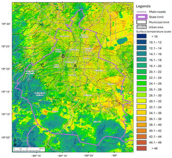
Figure 1.
Landsat (8 TIRS 2020/03/04) satellite image showing the distribution of surface temperature (°C) and the location of the modules studied in the districts of Narvarte (A), Escandón (B) and Santa Fe (C).
Three modules were selected within Mexico City: Narvarte (19°22′57″ N, 99°09′00″ W, 2240 m asl; area 99 m × 150 m; NAR), Escandón (19°24′15″ N, 99°10′34″ W; 2261 m asl; area 145 m × 116 m; ESC) and Santa Fe (19°21′36″ N, 99°16′08″ W; 2702 m asl; area 1016 m × 244 m; SFE). Land use in the three modules is given in Table 1. NAR and ESC exhibit similar architectural structures, mainly red surfaces such as red acrylic waterproofing and gray surface concrete roof cover, respectively (Figure 2A,B); however, NAR contains more light colors (white paint surface density and beige) than ESC. The material construction in SFE contains white surfaces (white acrylic waterproof) and glass in all buildings (Figure 2C).

Table 1.
Land use in each of the three modules, Narvarte (NAR), Escandon (ESC) and Santa Fe (SFE) in Mexico City.
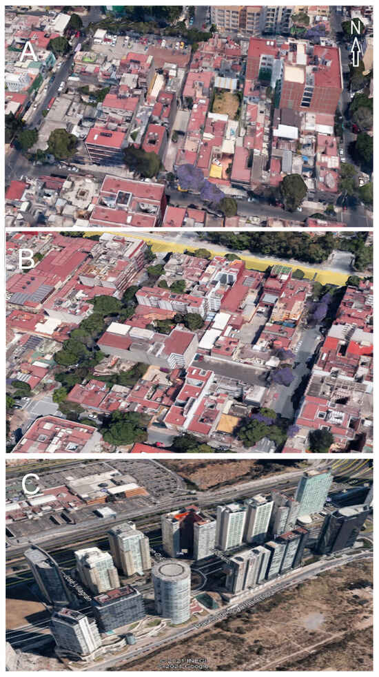
Figure 2.
Three-dimensional images of the selected blocks as depicted by Google Earth Pro: Narvarte (A), Escandón (B), and Santa Fe (C).
2.3. Module Parameters
Morphology was calculated in each module to determine building width and height corresponding to the block area and urban geometry (forms and discontinuities) to determine the soil cover. The dimensions of the block were thus obtained to establish the total area of the module and the planar area that corresponded to the area of the building envelope. Information georeferenced was obtained from Google Earth Pro, which helped to localize the modules in the INEGI web page, where zoned characteristics such as parks, urban areas, building land use (commercial, habitational, etc.), and the surrounding neighborhood information are given [37]. To classify land use, it was necessary to apply the “grid method”, which helped to determine the vegetal cover and “residue” corresponding to the habitational type and arrive at the land-use allocation classification.
Urban density was estimated from the dimensionless relationships proposed by Oke et al. [38], which determine how densely urbanized a given area is. Climatologically, the city’s morphology is characterized regarding the height, width, and density of its buildings. Grimmond and Oke [39] defined this morphometry of the study area (AT) as surface dimensions as follows:
where λF and λP denote the densities of the frontal and plane constructions, respectively; AP is the flat area of the element; AF is the front (vertical) area of the element; LX and LY are the length and width of the element, respectively; DX is the length and DY is width of the total area (including trees, streets, and other elements); and ZH is the height of the element. This characterization is not limited and may include houses of different shapes, winding streets, and dispersed trees that are typical of cities. These parameters were obtained using the Google Earth Pro program, with which the morphometry of the study sites was prepared.
λP = APAT = LXLY/DXDY and λF = AFAT = ZHLY/DXDY
From Equation (1), only λP was used for urban density since it defines the density in a given area horizontally. To obtain λP for a given site, blocks were characterized based on their shared physical characteristics, mainly length and width. Three study sites were described: NAR, ESC, and SFE, with a radius of 1.5 km around the micrometeorological stations that comprise the different forms of urban planning and land use. The characterization consisted of typical blocks within the study sites utilized to obtain the main urban parameters.
We estimated aerodynamic resistance using the formulation of the logarithmic wind profile on rough surfaces typical of cities as follows:
where rA is the aerodynamic resistance, u is the wind speed, k is the von Karman’s constant (≈0.41), ZW is the height where wind was measured, Z0 is the roughness length and d is the height of zero displacement height.
2.4. Computational Fluid Dynamics
Three-dimensional computer simulations of the three selected modules in Mexico City were performed using Ansys Fluent software 2019 R2. Ansys Fluent is a computational fluid dynamics (CFD) program. This software is a critical tool to optimize heat exchange performance by selecting the most appropriate materials and predicting durability and duration. Heat exchanger simulation application capabilities provide reliability, conjugate heat transfer, and can include fluid–structure interaction [40]. CFD models are capable of resolving physical phenomena, can reproduce the detailed microclimate in a neighborhood, and are coupled with models to analyze the physical environment within the city [10]. The Ansys Fluent model was applied to analyze thermal fluxes, w, and energy transport.
Three-dimensional solid prototype models were built using AutoCAD 2016 software. Model images, widths, heights, and the superficial areas of buildings were obtained from Google Earth Pro software 2022. Modules were exported to a .SAT extension file and imported into Ansys Design Modeler.
Domain discretization was employed with the “meshing tool”, using a hexahedral Cartesian mesh (Table 2). The values in Table 2 indicate that the number of mesh elements was appropriate, since the orthogonal quality values were very close to 1, which demonstrates that the flow, turbulence, and heat transfer are faithfully represented and errors are minimal. Although the bias values were low for Escandon and Santa Fe, we had a good quality mesh with a refinement concentrated towards the end of the domain.
Table 2.
Characteristics of the mesh or computational domain corresponding to the three modules under study: Narvarte Escandon and Santa Fe in Mexico City.
To obtain the wind speeds and temperatures within the domain, the equations of motion were solved using Ansys Fluent with boundary conditions given by the ambient temperature, wind speed, and radiative properties of the surfaces.
2.4.1. Processing Characteristics
Characteristics Considered for Analysis to Model Processing in Ansys Fluent
Since we used CFD software to simulate the turbulence and temperatures of the modules under study, we selected the following steps from the model:
- Temporal formulation: Transient state, analysis every hour.
- The orientation of the mesh: North-“x”, east- “z”, and gravity acceleration- “z”.
- Radiation: Surface to surface (S2S) with solar change calculated from the geographical coordinates of the chosen study sites, date, and hour of analysis.
- Turbulence: Dissipation model of k-epsilon energy with improved wall treatment.
- Analysis with heat transfer employing the energy equation and density modeled with the ideal gas law, which is not comprehensible for the density calculation.
Wind behavior was decomposed into north, south, east, and west, with an incidence angle (θw) and its velocity ():
Wind Data to Ventilation Analysis in Spaces with Ansys and Calibration
Natural ventilation analysis in building envelopes requires valid data to determine the real distribution of the ventilation in all gaps in the building because, in the envelope, wind direction as well as the global radiation are constantly changing in the gap. For this reason, the analysis was designated as “transient”. Wind and temperature data were obtained from the RedMet, as well as the geographical coordinates and urban characteristics of the neighborhood.
Radiative Properties
The thermal properties of urban construction material in combination with the three-dimensional geometry of built-up surfaces can modify neighborhood air temperatures. The thermal inertia of urban material construction is greater than in rural environments [41]. For this, we considered the radiative properties of every element (building) in the module, and the types of albedos of superficial radiative properties were analyzed.
Each building contained in each module was listed (Table 3). Each building was classified as walls and roofs, and these were assigned their radiative property. In addition, each element contained in the walls and roofs was considered and classified. A number was assigned to each building according to the coloration and analogies of its radiative properties.
Table 3.
Radiative properties of the material compilation of all wall and roof construction elements for each module analyzed. The glass values presented correspond to 6 mm thick glass [42].
2.4.2. Simulation Model Validation
Simulations for all modules were made hourly and calibrated with data measurements from the Meteorological Network (RedMet) in Mexico City (SIMAT, 2022). These simulations corresponded to the highest and the lowest temperatures registered during the year of analysis for the selected module (5 January and 23 March 2020) from 06:00 to 19:00 local time (LT). Data was collected from the station nearest to the point of the module: ESC from Miguel Hidalgo station, NAR from Benito Juarez station, and SFE from Santa Fe station. A comparison was made between the RedMet air temperatures and those generated by the Ansys Fluent model during at least 15 iterative steps of one hour each. A regression analysis of the air temperature generated by the model TM against the temperature measured by the RedMet instrumentation (TA) gave the following formulation: TM = 0.90007TA + 2.308; r2 = 0.988, p < 0.05; the RMSE was 0.67 °C, and a fairly small relative error of 3% was found.
2.4.3. Statistical Analysis
The results of the temperature simulations were plotted using images from the three modules. The Surfer program (Golden software 19.2) was useful when creating isotherm contours, applying kriging interpolation, and on top surface maps. We used a one-way ANOVA (T or w) without interactions, since the comparisons were always made at the same time, and we applied an F test, using p < 0.05 as significant, to compare all temperature and wind speed simulation results. Graphs were made using the Sigma Plot 12.0 statistical program.
3. Results and Discussion
3.1. Radiative Properties or Spectrophotometry
Each element found in the roof of each building comprising the module was quantified by color or by construction material, with the purpose of determining radiative behavior as solar absorptance and infrared emittance. Radiative properties are an important variable, and Ansys Fluent input conditions to calculate the temperature and wind behavior in the building envelope in the simulations. ESC roofs were made of 44.4% gray material as concrete; 40.3% red waterproof acrylic; 8.3% white waterproof acrylic; 2.8% beige color; and 1.4% each of orange to yellow, copper, and brown linoleum. NAR roofs were made of 34.2% red waterproof acrylic, 40.8% gray concrete material, 11.8% white waterproof acrylic, 7.9% beige color, and 2.6% each of brown and pinkish linoleum.
SFE consists of 17.9% white waterproof acrylic, 46.2% gray material or concrete, 25.6% red waterproof acrylic, and 5.1% each of beige and crystal material. This information, along with that contained in Table 4, was used to perform the simulations, representing the model constitution of the modules.
Table 4.
Urban aerodynamic parameters in each module.
3.2. Air Temperature Behavior, Numerical Simulation
Figure 3 shows the average temperature distribution in the three modules studied, NAR, ESC, and SFE. The temperature for ESC ranged in March from 23.6 to 24.9 °C with an average temperature of 24.3 °C. Average building roof temperatures were significantly different (F(37, 1025) = 10.0, p = 0.000). The average roof temperatures in January also differed (F(37, 1025) = 16.26, p = 0.000). Roof temperatures ranged from 14.1 to 12.9 °C (13.5 °C average roof temperature).
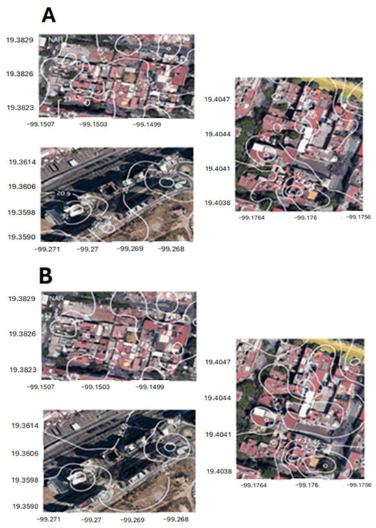
Figure 3.
Temperature distribution simulations (°C) on the roofs of the modules in (A) 23 March 2020, and (B) 6 January 2020. Modified from Google Earth Pro.
NAR roof temperatures also differed between buildings (F(37, 1025) = 12.45, p = 0.000); in January, roof temperatures ranged from 12.6 to 13.4 °C with an average temperature of 13.0 °C, while in March roof temperatures ranged from 22.7 to 23.6 °C with an average temperature of 23.1 °C (F(37, 1025) = 8.67, p = 0.000).
For SFE, roof temperatures also varied. In January, values ranged from 10.7 to 11.6 °C with an average temperature of 11.2 °C (F(15, 430) = 10.39, p = 0.000), and in March, roof temperatures ranged from 20.2 to 21.3 °C (F(37, 1025) = 8.80, p = 0.000).
Temperatures near 23.0 °C were mainly located on concrete roofs. On the NAR roofs, temperature differences were as high as 1.0 °C (22.7 to 23.6 °C). The lowest temperature corresponded to the gray material. On the northeast side, temperatures reached 22 °C, coinciding with an 18 m high building where the temperature rose to 23.5 °C, as well as on the south side, with buildings from 10 to 14 m high. In SFE, the highest simulated temperature (21.3 °C) was near the lowest temperature in the other two modules. The temperature varied between 20.2 and 21.3 °C (a difference of 1.5 °C). The lowest temperature was found near the street (in what would be the canyon), coinciding with the shadows generated by the buildings on the south-facing facades. Upon exiting the canyon, we encountered higher temperatures related to buildings made of materials such as glass and with white paint on the facades. However, when solid materials were encountered, they were painted white or black, resulting in temperatures ranging from 21.0 to 21.3 °C (Figure 3).
Air roof temperatures (ΔTA-R) also varied (F(2, 4515) = 54.59, p = 0.000) with averages of −0.77, −0.54, and −0.47 °C for NAR, ESC, and SFE, respectively, indicating that the building roofs were colder than the air. Although the temperature differences were small, these values indicate a clear cooling effect on the roofs due to turbulence.
The results showed that the highest temperature recorded for SFE was also the lowest for NAR. Only results for 23 March 2020, at 15:00 LT, are presented, as all other scenarios were very similar, and this was also the month with the highest temperatures (Figure 4). There were remarkable temperature differences between colored roofs on the one hand, and the gray and white roofs on the other hand, which behaved similarly, with a temperature 1 °C lower than the main simulation record (24.9 °C) for the red roof. Moreover, the temperature inside and around buildings was lower for SFE (30.0 °C) than ESC (33.0 °C), and NAR had an intermediate temperature (32.0 °C). It is also relevant to note that the structures for SFE were distinct between the three modules, as they were made primarily of glass walls, but all buildings were, of course, reinforced with concrete, mostly painted white.
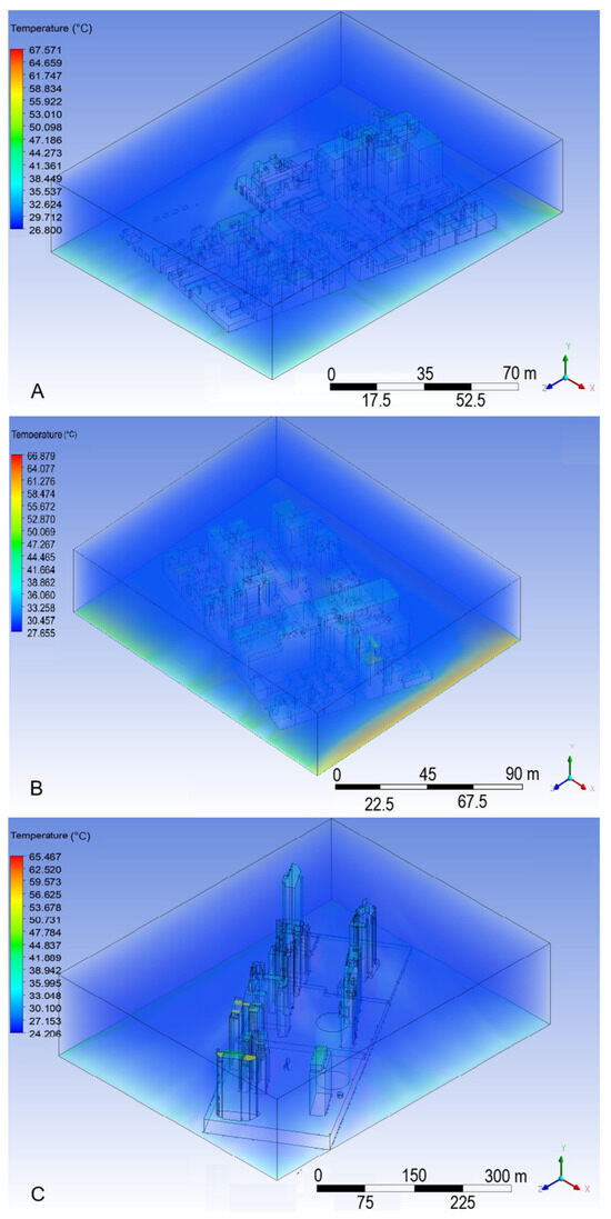
Figure 4.
Ansys Fluent temperature field output at 15:00 LT on 23 March 2020, in the Narvarte (A), Escandón (B), and Santa Fe (C) modules.
Figure 4 shows one of the outputs of the temperature distribution across the entire domain on March 23rd at 15:00 LT (one of the warmest months and the highest daily temperature near the maximum temperature of the day). In the Narvarte domain, the temperature was approximately 28 °C, and the roof temperatures ranged from 35 to 46 °C. The highest temperatures (>41 °C) were localized on the northern part of the module, and apparently, the height of the buildings did not influence these temperatures. However, it can be noted that a building approximately 20 m high obstructs the passage of solar radiation, shading another building. It is worth noting that the roof may be brown, white, or red, with brown predominantly affecting its temperature (Figure 4A). The temperature recorded in the Escandon module was approximately 30 °C, while roof temperatures ranged from 18 to 50 °C, especially in the southern part of the module. Although this module was located next to a wide, open avenue, the highest temperatures (>47 °C) were concentrated in the tallest buildings in the southern area of the module (Figure 4B). In Santa Fe, the domain temperature was 27 °C, and the warmest roofs were located on the west side with temperatures ranging from 40 to 53 °C, with no apparent effect of the radiative properties. Notably, the more open solar path in Santa Fe allowed these roofs to experience higher temperatures than the other two modules, as they received unobstructed solar radiation throughout the day (Figure 4C). The radiative characteristics of the roofs apparently did not matter in any of the three modules but rather depended more on the daytime solar path.
3.3. Vertical Wind Behavior
Wind simulations indicated how turbulence was present in all modules but was slightly higher in NAR. These turbulences were caused by two factors: first, differences or discontinuities in the building heights, and, second, radiative differences in the construction materials. Turbulence in the ESC module was presented mainly between a 20 m high building (Figure 5B, referenced position points 15, 16, 17) and a 9 m high building (Figure 5B, referenced position 20), together with their red and gray roof radiative characteristics. In NAR, one building (Figure 5B position 32) was 20 m high and experienced turbulence with its neighboring building 23 (Figure 3B, 6 m high), which had another tall neighboring building (36, 5 m high). In Figure 3B, position 36 has a gray roof with a gray parking lot, and positions 32 and 39 have red roofs, as well as building 23. SFE was totally different because all buildings were very tall (averaged at 91 m high); the wind blows from the northwest and exerts a dragging motion across the street canyon, where the turbulence appears at a great height. Because the distance between buildings was wide (east to west), the turbulence was stronger, and in the street canyon, the wind takes a higher speed towards the west side (Figure 5; Figure S1).
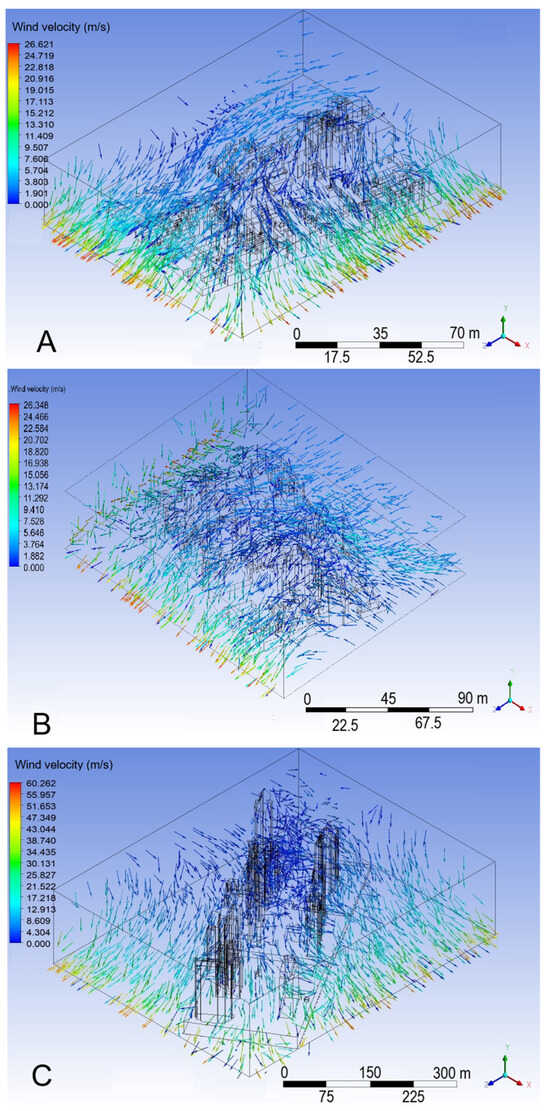
Figure 5.
Ansys Fluent wind field output at 15:00 LT on 23 March 2020, in the Narvarte (A), Escandón (B), and Santa Fe (C) modules.
Figure 6 shows the intensity of w in the modules studied, where it can be observed that w was more intense in the NAR module, with intensities of up to 7.7 m·s−1 in March at point 7, while in January, the value was almost 7.0 m·s−1. It is noteworthy that the positive values predominated in different positions on the roof. Only six points with negative values were presented (points 20, 32, 34, 36, 38, and 40, Figure S1), the highest being −0.73 m·s−1. In the ESC module, there were also values of up to 3.85 and 2.07 m·s−1 in March and January, respectively, at point 10. In general, w was different in the three sites, suggesting non-homogeneous groups, with differences of −0.353 m·s−1 between ESC and NAR, 1.74 m·s−1 between ESC and SFE, and 2.09 m·s−1 between NAR and SFE (F(2,6508) = 383; p < 0.000), and averages of 0.9, 0.56, and −1.19 m·s−1 in NAR, ESC, and SFE, respectively. Note the signs of w, two of which were positive (NAR, ESC) and one negative (SFE), indicating that in NAR and ESC the air rises, transporting heat to the upper layers of the atmosphere, while in SFE it descends, transferring the heat to the sides of buildings. This behavior likely led to greater cooling in NAR and ESC than in SFE, mainly due to mechanical turbulence, as shown in Figure 5 and Figure 6.
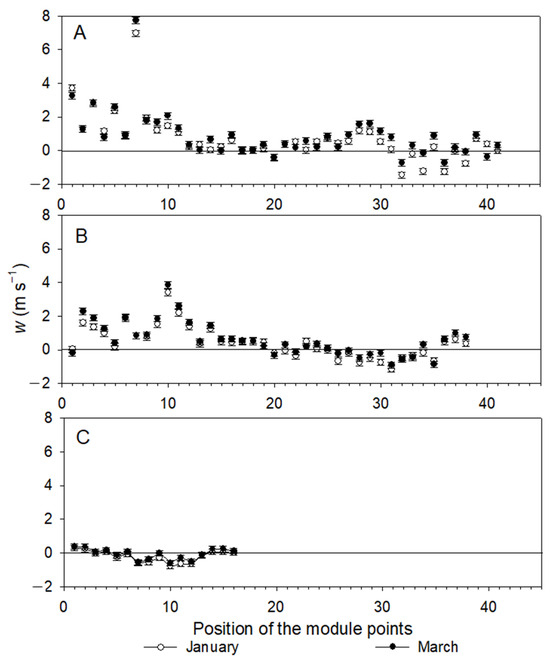
Figure 6.
Calculated w between building roof points in Narvarte (A), Escandón (B), and Santa Fe (C). Open and closed symbols correspond to 6 January and 23 March (see Supplemental Figure S1 for the point positions).
It is also possible to observe in Figure 6 that the highest values of the w wind speed were higher at the given position points between 1 and 10 and from 24 to 31 in NAR and from 1 to 15 in ESC, which coincided with large discontinuities in the structure of the building complex of the modules, while in SFE the structure was more homogeneous (Figure S1). Although NAR and ESC were similar in their dynamic characteristics (Table 4), it is important to note that the disposition of NAR against the wind direction presented a high building barrier, emulating a windbreak, thereby making the turbulence greater in NAR than in ESC. The aerodynamic characteristics of the SFE module were evident in its height (z), which was up to 12-fold higher than that of the NAR and ESC modules. This gave it a much higher roughness length (z0) and zero displacement (d), suggesting that turbulence was lower and negative in the SFE, as observed in Figure 6.
To our knowledge, this research is groundbreaking when applied to mitigating concentrated heat in cities. Some studies, such as Shirzadi and Tominaga’s [43], have used Ansys Fluent to analyze a scaled-down set of buildings that could easily be city blocks or fully enclosed towers without protrusions or cavities and only showed surface currents and the effect of a tall tower. Using four fully enclosed buildings of the same height, Gagliano et al. [44] studied the mitigation of UHIs with CFD by analyzing the spaces between the buildings (street canyons) with apparently good results for the temperature of the facades. Furthermore, the studies carried out on urban microclimates that include CFD have been mainly limited to urban canyons, completely open spaces, and blocks with multiple buildings with generic structures [45].
These results can support the first step in building an urban landscape that mitigates the heat from both buildings and the air. Wind and turbulence increase convective exchange and evacuate the accumulated heat in the distributions of buildings that make up a block, reducing their temperatures. According to the temperature reductions of the NAR module, this effect is due to the great discontinuity presented by this architectural arrangement. The air temperature is reduced at the block scale where buildings act as windbreakers and also in concavities that reach the surface level, increasing turbulence, as shown in position points 5, 6, 7, and 8 (Figure S1), where w reaches a speed of up to 7 m·s−1. This demonstrates that air turbulence is a passive way of cooling buildings and that it depends on their architectural characteristics, although it seems that the vertical structure is not as important as the horizontal one and that it not only requires a set of buildings of different heights, but also cavities or hollows. Thus, the construction of the urban landscape must be such that it increases the heat flux mainly upwards, which can be achieved using architectural projects similar to the NAR design. However, this design was achieved completely at random since, as the city grew, buildings were added in the different districts according to the legal requirements of the time in which they were built. By increasing positive w, it is also possible to mitigate the urban heat island effect since by dragging heat upwards, surfaces are cooled, in this case, the roofs of buildings.
The results from one city should not be generalized to others; they should be adapted to each climate and urban environment studied [10]. However, landscape elements must be considered in the planning process for their effectiveness in reducing temperature to achieve human thermal comfort [46,47,48,49]. One advantage of environmental analysis through simulations with microclimate models is that it leads to evaluating the best mitigation method to apply in a region and selecting the most appropriate method to be devised, approved, and implemented [50]. This will not only encompass the heat flows in the modules already stipulated but will also incorporate the design where the appropriate turbulence is generated to achieve the greatest possible cooling, contributing to mitigating/adapting to the urban heat island, thus leading to a more sustainable city.
4. Conclusions
As we have shown, turbulence can affect the modules’ cooling. The discontinuity in module morphology is as significant regarding building height as the distance between the buildings, generating turbulence that significantly increases w. In the case of SFE, we only considered the distances between buildings; however, in ESC and NAR, we observed how the parking areas create turbulence as areas of discontinuity, which was greater in NAR due to a current windbreak. This information is valuable and can help us increase ventilation and the transport of heat and pollutants. It is important to locate parking outside and/or next to buildings, regardless of their height. Another recommendation is to build a mixed configuration of high and low buildings to increase turbulence and to consider albedos. The color difference can decrease the temperature up to 1 °C. This information will facilitate adapting to UHI, decreasing air temperature, and improving our health and air quality through pollutant transportation.
It is important to note that w depends on the building structures and construction materials or radiative properties of each module. It is necessary to consider UHI mitigation in urban planning by making adequate use of urban elements in module arrangements to generate greater heat exchange.
Supplementary Materials
The following supporting information can be downloaded at: https://www.mdpi.com/article/10.3390/land14102013/s1, Figure S1. Distribution of the different position points on the roofs of the buildings in the Narvarte (A), Escandon (B) and Santa Fe (SFE) modules as “seen” by Ansys Fluent model. Modified from Google Earth Pro.
Author Contributions
Conceptualization, M.B., V.L.B., A.L.-O. and J.G.O.S.; methodology, M.B., V.L.B. and A.L.-O.; software, M.B. and S.R.S.V.-M.; validation, S.R.S.V.-M.; formal analysis, M.B., V.L.B. and A.L.-O.; investigation, M.B., V.L.B., A.L.-O., S.R.S.V.-M. and J.G.O.S.; resources, A.L.-O. and J.G.O.S.; data curation, M.B., V.L.B. and S.R.S.V.-M.; writing—original draft preparation, M.B. and V.L.B.; writing—review and editing, M.B. and V.L.B.; supervision, A.L.-O. and J.G.O.S.; project administration, A.L.-O. and J.G.O.S.; funding acquisition, A.L.-O. and J.G.O.S. All authors have read and agreed to the published version of the manuscript.
Funding
This work was supported by Universidad Nacional Autónoma de México Postdoctoral Program (Posdoc).
Data Availability Statement
The original contributions presented in this study are included in the article/Supplementary Material. Further inquiries can be directed to the corresponding authors.
Acknowledgments
The first author thanks Universidad Nacional Autónoma de México Postdoctoral Program (Posdoc). We would like to thank Pablo Leautaud for his technical support in the analysis of satellite images.
Conflicts of Interest
The authors declare no conflicts of interest.
References
- Solecki, W.D.; Rosenzweig, C.; Parshall, L.; Pope, G.; Clark, M.; Cox, J.; Wiencke, M. Mitigation of the heat island effect in urban New Jersey. Glob. Environ. Change Part B Environ. Hazards 2005, 6, 39–49. [Google Scholar] [CrossRef]
- Díaz, M. Cálculo del Cambio de Temperatura Atmosférica Debido al Cambio de Albedo. Aplicación Para la Ciudad de México Mediante la Implementación de “Techos Verdes”. Bachelor’s Thesis, Facultad de Ciencias, UNAM, Mexico City, Mexico, 2008. [Google Scholar]
- Chandler, T.J. London’s urban climate. Geogr. J. 1962, 8, 279–298. [Google Scholar] [CrossRef]
- Oke, T.R. The heat island of the urban boundary layer: Characteristics, causes and effects. In Wind Climate in Cities, 1st ed.; Cermak, J.E., Davenport, A.G., Plate, E.J., Viegas, D.X., Eds.; Springer: Dordrecht, The Netherlands, 1995; Volume 277, pp. 81–197. [Google Scholar]
- Santamouris, M.; Synnefa, A.; Karlessi, T. Using advanced cool materials in the urban built environment to mitigate heat islands and improve thermal comfort conditions. Sol. Energy 2011, 85, 3085–3102. [Google Scholar] [CrossRef]
- Ballinas, M.; Barradas, V.L. The urban tree as a tool to mitigate the urban heat island in Mexico City: A simple phenomenological model. J. Environ. Qual. 2016, 45, 157–166. [Google Scholar] [CrossRef] [PubMed]
- Ballinas, M. Mitigación de la Isla de Calor Urbana: Estudio de Caso de la Zona Metropolitana de la Ciudad de México. Master’s Thesis, Centro de Ciencias de la Atmósfera-Instituto de Ecología, UNAM, Mexico City, Mexico, 2011. [Google Scholar]
- Jauregui, E. Impact of land-use changes on the climate of the Mexico City region. Investig. Geogr. 2012, 46. [Google Scholar] [CrossRef]
- Valger, S.A.; Fedorova, N.N. Numerical simulation of heat and mass transfer in air in vicinity of bluff body. J. Phys. 2018, 1105, 12–17. [Google Scholar] [CrossRef]
- Hayes, A.T.; Jandaghian, Z.; Lacasse, M.A.; Gaur, A.; Lu, H.; Laouadi, A.; Ge, H.; Wang, L. Nature-based solutions (nbss) to mitigate urban heat island (UHI) effects in Canadian cities. Buildings 2022, 12, 925. [Google Scholar] [CrossRef]
- Takebayashi, H.; Okubo, M.; Danno, H. Thermal environment map in street canyon for implementing extreme high temperature measures. Atmosphere 2020, 11, 550. [Google Scholar] [CrossRef]
- Hong, T.; Xu, Y.; Sun, K.; Zhang, W.; Luo, X.; Hooper, B. Urban microclimate and its impact on building performance: A case study of San Francisco. Urban Clim. 2021, 38, 100871. [Google Scholar] [CrossRef]
- Coutts, A.M.; Beringer, J.; Tapper, N.J. Impact of increasing urban density on local climate: Spatial and temporal variations in the surface energy balance in Melbourne, Australia. J. Appl. Meteorol. Clim. 2007, 46, 477–493. [Google Scholar] [CrossRef]
- Pattacini, L. Climate and urban form. Urban Des. Int. 2012, 17, 106–114. [Google Scholar] [CrossRef]
- Baklanov, A.; Molina, L.T.; Gauss, M.M. Megacities, air quality and climate. Atmos. Environ. 2016, 126, 235–249. [Google Scholar] [CrossRef]
- Ryu, Y.H.; Baik, J.J.; Lee, S.H. A new single-layer urban canopy model for use in mesoscale atmospheric models. J. Appl. Meteorol. Clim. 2011, 50, 1773–1794. [Google Scholar] [CrossRef]
- Barradas, V.L. Evidencia del efecto de la isla térmica en Jalapa, Veracruz, México. Geofisica 1987, 26, 125–135. [Google Scholar]
- Ballinas, M.; Barradas, V.L. Transpiration and stomatal conductance as potential mechanisms to mitigate the heat load in Mexico City. Urban For. Urban Green. 2016, 20, 152–159. [Google Scholar] [CrossRef]
- Bonifacio-Bautista, M.; Ballinas, M.; Jazcilevich, A.; Barradas, V.L. Estimation of anthropogenic heat release in Mexico City. Urban Clim. 2022, 43, 101158. [Google Scholar] [CrossRef]
- Kumar, P.; Debele, S.E.; Khalili, S.; Halios, C.H.; Sahani, J.; Aghamohammadi, N.; de Fatima Andrade, M.; Athanassiadou, M.; Bhui, K.; Calvillo, N.; et al. Urban heat mitigation by green and blue infrastructure: Drivers, effectiveness, and future needs. Innovation 2024, 5, 100588. [Google Scholar] [CrossRef]
- Irfeey, A.M.M.; Chau, H.W.; Sumaiya, M.M.F.; Wai, C.Y.; Muttil, N.; Jamei, E. Sustainable mitigation strategies for urban heat island effects in urban areas. Sustainability 2023, 15, 10767. [Google Scholar] [CrossRef]
- Aboelata, A.; Sodoudi, S. Evaluating the effect of trees on UHI mitigation and reduction of energy usage in different built-up areas in Cairo. Build. Environ. 2020, 168, 106490. [Google Scholar] [CrossRef]
- Internacional Energy Agency (IEA). Manual de Estadísticas Energéticas. Available online: https://www.iea.org/reports/energy-statistics-manual-2 (accessed on 15 July 2025).
- Ramos-Gutiérrez, L.D.J.; Montenegro-Fragoso, M. La generación de energía eléctrica en México. Tecnol. Cienc. Agua 2012, 3, 197–211. [Google Scholar]
- Secretaría del Medio Ambiente de la Ciudad de México. Calidad del Aire en la Ciudad de México, Infograma: El Consumo Energético en la Ciudad de México. Dirección General de Calidad del Aire, Dirección de Monitoreo de Calidad del Aire. Available online: http://www.aire.cdmx.gob.mx/descargas/publicaciones/simat-infograma-consumo-energetico.pdf (accessed on 25 July 2025).
- Ramos, G.; Heard, C.; Viveros, A.S. Simulación de escenarios de ahorro y uso eficiente de energía con medidas de control pasivo. Rev. FIDE 1998, 7, 17–29. [Google Scholar]
- Ballinas, M.; Morales-Santiago, S.I.; Barradas, V.L.; Lira, A.; Oliva-Salinas, G. Is PET an adequate index to determine human thermal comfort in Mexico City? Sustainability 2022, 14, 12539. [Google Scholar] [CrossRef]
- Kosutova, K.; Van Hooff, T.; Vanderwel, C.; Blocken, B.; Hensen, J. Cross-ventilation in a generic isolated building equipped with louvers: Wind-tunnel experiments and CFD simulations. Build. Environ. 2019, 154, 263–280. [Google Scholar] [CrossRef]
- Geetha, N.B.; Velraj, R.J.E.E.S. Passive cooling methods for energy efficient buildings with and without thermal energy storage—A review. Energy Educ. Sci. Technol. Part A Energy Sci. Res 2012, 29, 913–946. [Google Scholar]
- Nikou, M.K.; Ehsani, M.R. Turbulence models application on CFD simulation of hydrodynamics, heat and mass transfer in a structured packing. Int. Commun. Heat Mass Transf. 2008, 35, 1211–1219. [Google Scholar] [CrossRef]
- Ahmad, A.H.; Abu Bakar, A.F.; Osman, S.A. CFD Analysis of Thermal Conditions and Airflow Patterns in Commercial Laundry Facility using ANSYS Fluent Simulation. J. Adv. Res. Fluid Mech. Therm. Sci. 2025, 126, 106–126. [Google Scholar] [CrossRef]
- Li, Y.; Nielsen, P.V. CFD and ventilation research. Indoor Air 2011, 21, 442–453. [Google Scholar] [CrossRef]
- Thordal, M.S.; Bennetsen, J.C.; Koss, H.H.H. Review for practical application of CFD for the determination of wind load on high-rise buildings. J. Wind. Eng. Ind. Aerodyn. 2019, 186, 155–168. [Google Scholar] [CrossRef]
- Mittal, H.; Sharma, A.; Gairola, A. A review on the study of urban wind at the pedestrian level around buildings. J. Build. Eng. 2018, 18, 154–163. [Google Scholar] [CrossRef]
- Instituto Nacional de Estadística y Geografía (INEGI). Aspectos Geográficos de Ciudad de México: Compendio 2022. Ciudad de México. 2022. Available online: http://www.inegi.org.mx/contenidos/productos/prod_serv/contenidos/espanol/bvinegi/productos/nueva_estruc/889463912972.pdf (accessed on 30 July 2025).
- Servicio Meteorológico Nacional (SMN). Normales Climatológicas. Ciudad de México. 2025. Available online: https://smn.conagua.gob.mx/es/climatologia/informacion-climatologica/normales-climatologicas-por-estado (accessed on 15 July 2025).
- Instituto Nacional de Estadística y Geografía (INEGI). Síntesis Metodológica y Conceptual de la Infraestructura y Características del Entorno Urbano del Censo de Población y Vivienda 2010; INEGI: Ciudad de México, Mexico, 2019. [Google Scholar]
- Oke, T.R.; Cleugh, H.A. Urban heat storage derived as energy balance residuals. Bound.-Layer Meteorol. 1987, 39, 233–245. [Google Scholar] [CrossRef]
- Grimmond, C.S.B.; Oke, T.R. Aerodynamic properties of urban areas derived from analysis of surface form. J. Appl. Meteorol. 1999, 38, 1262–1292. [Google Scholar] [CrossRef]
- Ansys. Available online: www.ansys.com (accessed on 8 August 2025).
- Perera, N.G.R.; Samanthilaka, K.P.P.R. Effect of street canyon materials on the Urban Heat Island phenomenon in Colombo. In Proceedings of the Conference Cities, People Places—ICCPP-2014, Colombo, Sri Lanka, 31 October–2 November 2014. [Google Scholar]
- Hernández Bernardino, J.C. Análisis Integral de Materiales de Azotea, Para la Construcción de Una Política Pública de Mitigación de la Isla de Calor Urbana, para la Ciudad de México, un Enfoque Desde la Sostenibilidad. Master’s Thesis, Posgrado en Ciencias de la Sostenibilidad, Instituto de Ecología, UNAM, Ciudad de México, Mexico.
- Shirzadi, M.; Tominaga, T. CFD evaluation of mean and turbulent wind characteristics around the Urban Heat Island. Build. Eviron. 2022, 225, 109637. [Google Scholar]
- Gagliano, A.; Nocera, F.; Aneli, S. Computational Fluid Dynamics analysis for evaluating the Urban Heat Island effects. Energy Procedia 2017, 134, 508–517. [Google Scholar] [CrossRef]
- Toparlar, Y.; Blockena, B.; Maiheub, B.; van Heijstd, G.J.F. A review on the CFD analysis of urban microclimate. Renew. Sustain. Energy Rev. 2017, 80, 1613–1640. [Google Scholar] [CrossRef]
- Yahia, M.W.; Johansson, E. Landscape interventions in improving thermal comfort in the hot dry city of Damascus, Syria—The example of residential spaces with detached buildings. Landsc. Urban Plan. 2014, 125, 1–16. [Google Scholar] [CrossRef]
- Yahia, M.W.; Johansson, E.; Thorsson, S.; Lindberg, F.; Rasmussen, M.I. Effect of urban design on microclimate and thermal comfort outdoors in warm-humid Dar es Salaam, Tanzania. Int. J. Biometeorol. 2018, 62, 373–385. [Google Scholar] [CrossRef]
- Salata, F.; Golasi, I.; de Lieto Vollaro, R.; de Lieto Vollaro, A. Urban microclimate and outdoor thermal comfort. A proper procedure to fit ENVI-met simulation outputs to experimental data. Sustain. Cities Soc. 2016, 26, 318–343. [Google Scholar] [CrossRef]
- Yang, W.; Lin, Y.; Li, C.Q. Effects of landscape design on urban microclimate and thermal comfort in tropical climate. Adv. Meteorol. 2018, 2809649. [Google Scholar] [CrossRef]
- Mohaher, H.R.H.; Ding, L.; Santamouris, M. Developing heat mitigation strategies in the urban environment of Sydney, Australia. Buildings 2022, 12, 903. [Google Scholar] [CrossRef]


Disclaimer/Publisher’s Note: The statements, opinions and data contained in all publications are solely those of the individual author(s) and contributor(s) and not of MDPI and/or the editor(s). MDPI and/or the editor(s) disclaim responsibility for any injury to people or property resulting from any ideas, methods, instructions or products referred to in the content. |
© 2025 by the authors. Licensee MDPI, Basel, Switzerland. This article is an open access article distributed under the terms and conditions of the Creative Commons Attribution (CC BY) license (https://creativecommons.org/licenses/by/4.0/).