Abstract
Quantitative analysis of ecosystem services (ESs) supply–demand dynamics, and identifying its dominant drivers and the spatial non-stationarity of driving mechanisms, is a crucial prerequisite for effective regional ESs management and the formulation of scientific ecological conservation plans. Previous related studies have primarily focused on the supply–demand balance of specific ESs and the driving analysis of ESs supply. Comprehensive analysis of ESs supply–demand dynamics and research on their spatially heterogeneous response mechanisms remain relatively scarce. In this study, we assessed the supply, demand, and supply–demand matching relationships of ESs on the Loess Plateau (LP) from 1990 to 2023 using a land-cover-based ESs supply–demand quantitative matrix. We then employed Geodetector and Geographically weighted regression model to explore the dominant driving factors and their spatially varying effects on ESs supply–demand relationships. The results revealed that over the past three decades, the continuous decline in ESs supply coupled with the annual increase in ESs demand has led to a worsening trend in ESs supply–demand relationships towards deficit. Fortunately, the LP still maintained a supply-surplus state at present. The proportion of construction land, population density, GDP density, and the proportion of forestland and grassland were identified as key drivers of changes in ESs supply–demand relationships. The expansion of construction land was the most crucial driver of the deterioration in ESs supply–demand relationships on the LP, exhibiting a universally negative inhibitory effect. The proportion of forestland and grassland exerted a regionally wide positive spatial effect, highlighting the critical role of vegetation restoration in improving ESs relationships. The influences of population density and GDP density exhibited a coexistence of positive promoting and negative inhibitory effects across space. Our results emphasize that ESs management policies on the LP must account for the spatial heterogeneity of driving mechanisms, requiring more localized and targeted land use strategies and management policies to enhance ESs sustainability.
1. Introduction
The sustenance and enhancement of human well-being fundamentally rely on the diverse benefits provided by natural ecosystems [1,2], known as ecosystem services (ESs). In the process of entering the “Anthropocene”, living standards are gradually improving, and the sense of well-being derived from ecological benefits is increasing [3,4]. However, it is undeniable that with global population growth, economic expansion, and accelerated urbanization, the total volume and diversity of societal demands for ESs are also escalating [5,6,7]. Simultaneously, multiple pressures including land-cover change, over-exploitation of natural resources, environmental pollution, and climate change are causing significant degradation in ecosystem structure and function, threatening their capacity to sustainably provide ESs [8,9]. Empirical evidence indicates that approximately 60% of global ESs are in decline [10], while total human demand has surged by over 300% in the past 50 years [11]. This has triggered an increasing imbalance between ESs supply and demand, which will further impact the realization of the Sustainable Development Goals aimed at global shared prosperity, human well-being, and planetary sustainability [12]. The global imbalance in ESs supply–demand has evolved into a core contradiction threatening regional security and sustainable development [13]. Against this backdrop, conducting research on the dynamics of regional ESs supply–demand matching relationships and further revealing their underlying driving mechanisms is of paramount importance for coordinating ecological conservation and social development and enhancing ecosystem management effectiveness.
ESs supply is generally defined as the various products and services provided by the ecosystem to humans at a specific location and time [14], while ESs demand refers to the quantity of ESs consumed or desired by human society [15]. Although incorporating ESs demand into ESs assessment can help identify mismatches (in space and time) between ESs supply and demand and provide a basis for designing effective ESs management strategies [16], the past few decades have often seen more attention given to ESs supply [17,18]. Fortunately, with the development of quantitative methods for determining ESs supply and ESs demand, recent research has gradually shifted from quantifying ESs supply capacity to exploring ESs supply, demand, and their matching relationships [6,13,19].
Numerous methods have been developed to quantify ESs supply and demand. For instance, models like InVEST, RUSLE, CASA, and various empirical models are used to calculate the supply and demand of specific ESs such as water yield, soil retention, and carbon sequestration [20,21]. These models typically require extensive foundational data (e.g., meteorological, soil, land use, socio-economic data) for the assessment of specific ESs, and the involved model parameters are often complex and poorly transferable, making it difficult to achieve a comprehensive assessment of ESs supply–demand relationships [22]. Subsequently, a land-cover-based and expert-scoring-based ESs supply–demand quantitative matrix was proposed. This matrix incorporates a wider range of ESs types, enabling a more comprehensive quantification of ESs supply, demand, and supply–demand matching. It also facilitates cross-regional comparisons of ESs supply–demand situations and requires only land use data and the scoring matrix [23]. This method has proven to be a convenient and effective measurement tool both domestically and internationally, with well-received applications in countries including Germany [24], Thailand [25], Finland [26], Southeast Asia [27], and China [28,29,30].
ESs supply–demand matching relationship ultimately depend on the impacts of social–ecological drivers [2,15,16]. However, previous studies mostly stopped at the stage of supply–demand assessment, and further exploration of driving forces of supply–demand matching is still very limited [9,13]. Though researchers have recently realized this knowledge gap, these few existing studies are often limited to considering only natural ecological factors and lacking socio-economic factors [31], which may bring considerable uncertainty to ESs management decisions. In addition, since the uneven distribution of ESs across space, and factors that are potentially correlated, such as climate, terrain, socio-economy, etc., often vary with space, spatial heterogeneity of the ESs supply–demand or driving forces is inherent, that is, the property and intensity of the influence of the drivers affecting the ESs supply–demand matching relationship may vary in different spatial positions [9,31,32]. Therefore, current popular methods such as correlation analysis and ordinary multiple linear regression to reveal key influencing factors can only reflect the “average” or “global” status of the influence [9,20], masking the spatially differentiated response characteristics of supply–demand relationship to various driving factors, and thus cannot provide sufficient knowledge information for formulating regional spatial differentiation protection strategies.
The Chinese Loess Plateau (LP) is one of the regions in China where the contradictions between population, resources, and environment are most concentrated [33]. It is also the main area for implementing the major national strategy of ecological protection and high-quality development of the Yellow River Basin [34]. Consequently, it has become an ideal region for conducting ESs-related research and has yielded fruitful research outcomes. Unfortunately, to our knowledge, existing LP case studies have predominantly focused on the evolutionary trajectory of ESs from the supply side [20,35,36], rarely considering ESs supply–demand relationships, let alone further investigation into driving mechanisms. Therefore, addressing the deficiencies in the aforementioned field and focusing on the scientific needs of the LP, we selected the LP as the study target area to evaluate changes in ESs supply, demand, and supply–demand matching relationships, and further analyze the driving mechanisms of ESs supply–demand relationships on the LP. Specifically, the objectives of this study are as follows: (1) to evaluate the spatiotemporal characteristics of supply, demand, and supply–demand matching relationships for multiple ESs types on the LP over the past three decades using the land-cover-based ESs supply–demand quantitative matrix method; (2) to identify key driving factors of ESs supply–demand matching relationships changes by combining the Geodetector model; (3) to quantitatively reveal the spatially non-stationary response mechanisms of ESs supply–demand matching relationships to key driving factors by established Geographically weighted regression (GWR) model.
2. Materials and Methods
2.1. Study Area
The LP is located in northern China (Figure 1a), with a geographical coverage of 33°20′ N–41°43′ N and 100°41′ E–114°38′ E. It is the largest loess accumulation area in the world, encompassing 334 counties across seven provinces: Shanxi, Inner Mongolia, Henan, Shaanxi, Gansu, Ningxia, and Qinghai (Figure 1b). The land area is approximately 62.5 × 10⁴ km2, accounting for about 6.51% of China’s terrestrial area. The topography of the LP is complex. The northwestern part mainly consists of Agricultural irrigation region, sandy, and desert regions. The central part is dominated by loess hilly and gully region. The southwestern part features Loess Plateau gully region. The southeastern part primarily comprises River valley plain region, and the eastern part is mainly Rocky mountain region (Figure 1c). The terrain generally slopes from high in the northwest to low in the southeast, with elevation ranging from 61 m to 5208 m (Figure 1c). The climate of the LP is predominantly arid and semi-arid continental monsoon, with an average annual precipitation ranging from approximately 111 mm to 878 mm, decreasing from southeast to northwest (Figure 1d).
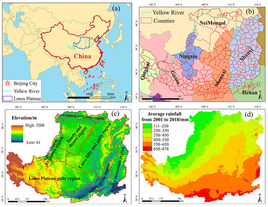
Figure 1.
Study area: (a) location of the LP, (b) administrative division, (c) elevation, (d) rainfall.
The LP serves as an important ecological barrier for the Yellow River Basin and is a vital component of China’s “Three Zones and Four Belts” ecological security strategic pattern. It plays a significant role in safeguarding the safety of the Yellow River and the North China Plain, as well as ensuring the security of energy base and food [33,34]. Simultaneously, the LP supports a population of 120 million people. Rapid economic development and accelerating urbanization have caused severe disturbance to the ecological environment, intensifying the contradiction between humans and land [37]. Therefore, evaluating ESs supply–demand matching relationships and improving ESs supply capacity are crucial for achieving sustainable development in this region.
2.2. Data Preparation
We collected land use data, foliage vegetation cove (FVC) data, digital elevation model (DEM) data, climate-related date and socio-economic data, all of which are sourced from authoritative data platforms and official publications in China. The details of data are presented in Table 1. It should be noted that our analysis was conducted within the county-level scale. In China, many formal ecological management decisions are made at the county-level scale. Therefore, we aggregated the latent social–ecological drivers at the grid scale to the “mean values” at county-level scale through Zonal Statistics tools in ArcGIS 10.2 platform.

Table 1.
Detailed description of the data.
2.3. Assessing ESs Supply, Demand, and Their Relationship
2.3.1. Measuring ESs Supply and Demand
Burkhard et al. pioneered the land-cover-based ESs supply–demand quantitative matrix [38], providing a simple, rapid, and effective method for quantifying ESs supply, demand, and their balance. This method has been widely applied by numerous scholars in ESs supply–demand relationship research [24,25,26,27,28,29,30,38], playing a significant role in advancing the concept of ESs from theoretical research to management practice. To enhance the applicability of the ESs supply–demand quantitative matrix, Jiang et al. scored the ESs supply and demand levels for secondary land use types specific to the LP [39], establishing an ESs supply–demand quantitative matrix tailored to the LP. Matrix scores range from 0 to 5, representing no relevance, extremely low, low, medium, high, and extremely high levels of ESs supply or demand, respectively. This matrix has effectively addressed the issue of the difficulty in unifying dimensions caused by the complexity and difficulty in obtaining ESs supply and human demand data, building a “bridge” for quantifying the relationship between ESs supply and human demand on the LP. This study, in combination with the research results of Jiang et al. [39], quantifies the supply and demand of ESs in the LP using the matrix shown in Figure 2. The calculation formula is as follows:
where ES, ED represent the ESs supply value and ESs demand value, respectively. Ek is the quantitative matrix values for ESs supply or ESs demand of land use type k. Sk is the area of land use type k.

Figure 2.
Quantitative matrix of ESs (a) supply and (b) demand for different land use types in the LP (after Jiang et al. [39]).
2.3.2. Sensitivity Test for Land-Cover-Based Approach
The sensitivity coefficient reflects the dependence of total ESs value to quantitative value and evaluates the rationality of the method. The sensitivity coefficient was calculated using Formula (2).
where SC is the sensitivity coefficient. VESa and VESb are the original and adjusted total ESs values, respectively. VLSa and VLSb are the original and adjusted quantitative values. The adjustment quantity was ±50%. The larger the SC, the higher the sensitivity of the total ESs values to quantitative values, that is, the stronger the uncertainty of the adopted quantitative matrix for the ESs supply and demand. If SC > 1, it indicates that the quantitative matrix for the ESs supply and demand we have adopted has unacceptable uncertainty. By contrast, if SC ≤ 1, it indicates that the uncertainty of the quantitative matrix we adopted is acceptable, which reflected that the method was reasonable [40].
2.3.3. Mapping ESs Supply–Demand Relationship
Based on the obtained ESs supply value and ESs demand values for each county of the LP, the ESs supply–demand matching index (ESSD), calculated using Equation (3), can be used to reflect the ESs supply–demand matching status in different counties of the LP.
where ESSD is the ESs supply–demand matching index. If ESSD > 0, it indicates supply exceeds demand (surplus state), if ESSD = 0, it indicates supply equals demand (balanced state), if ESSD < 0, it indicates supply is less than demand (deficit state).
2.4. Identifying Drivers of ESs Supply–Demand Relationship
2.4.1. Latent Social–Ecological Drivers Selection
Based on different systems and research purposes, the selection results of latent social–ecological drivers are often different. In our study, the latent social–ecological drivers were selected based on the following principles: (1) variables that directly or indirectly drive the ESs supply–demand matching relationship as identified in the relevant literature [9,32,39,40,41]; or (2) variables could reflect an important aspect of natural geography, climate, economy, society; plus (3) quantitative data for the variables had to be available. Ultimately, we selected eleven latent drivers that are important for determining the ESs supply–demand balance (Table 2).
Table 2.
Details of variables examined to investigate influences on ESs supply–demand matching relationship.
Figure 3 shows the spatial distribution of the selected drivers. It can be found that the dependent variable and the independent variables have obvious spatial heterogeneity, that is, the property and intensity of the influence of each independent variable on the dependent variable may vary at different spatial positions, which to some extent reflects the necessity of identifying the response characteristics of spatial differentiation for the dependent variable to the independent variables.
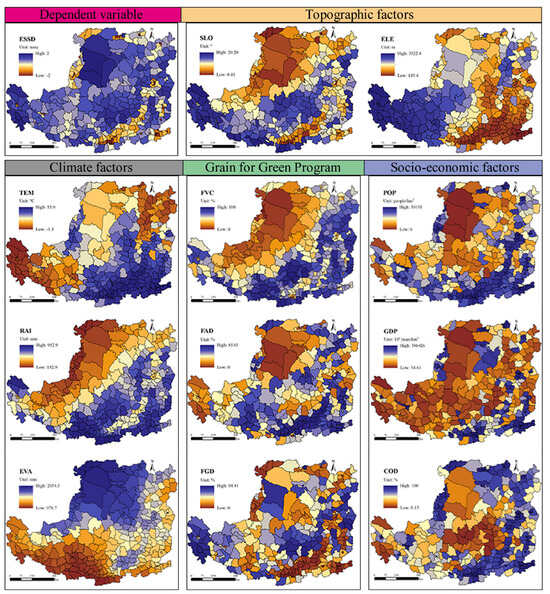
Figure 3.
Spatial distribution of the selected drivers on the LP (SLO: average slope; ELE: average elevation; TEM: annual average temperature; RAI: annual average rainfall; EVA: annual average evapotranspiration; FVC: foliage vegetation cover; FAD: proportion of farmland; FGD: proportion of forestland and grassland; POP: population density; GDP: GDP density; COD: proportion of construction land).
2.4.2. Geodetector
This study employed the Geodetector model [42] proposed by Wang and Xu to identify key driving factors of ESs supply–demand relationship changes in 2023. Geodetector is a novel statistical method based on spatial differentiation theory, utilizing spatial statistics to reveal underlying driving factors. It can analyze whether interactions exist between factors, as well as the strength, direction, linearity, and non-linearity of such interactions [43]. In this study, taking the ESSD for the year of 2023 as the dependent variable and the potential socio-ecological drivers as independent variables, we input them into the Geodetector for quantitative analysis of the influence of the driving factors. The model formula is
where represents the influence intensity of the latent socio-ecological driver on the ESs supply–demand matching relationship, with values ranging from 0 to 1. A larger q value indicates a stronger influence of the driver on the supply–demand matching relationship. is the number of strata of the variable. and are the number of samples in stratum and the total number of samples, respectively. and are the variance of stratum and the total variance of the entire region, respectively.
2.4.3. GWR Model
The GWR model is a local regression method based on Ordinary least squares that operate at different spatial scales [36]. It applies a spatial weight matrix to the linear regression model, allowing model coefficients to better explain the spatial heterogeneity of geographical elements and more effectively address the issue of spatial non-stationarity. Based on the results from the Geodetector model, we further employed the GWR model to reveal the spatial heterogeneity characteristics of the impact of several key influencing factors on the ESs supply–demand matching relationship. The model formula is
For county , is the ESSD. is the coefficient to be estimated. is the spatial geographic coordinate. is the influencing factor . is the random error term.
3. Results
3.1. Characteristics of ESs Supply and Demand
3.1.1. ESs Supply
Based on the ESs supply–demand quantitative matrix and land use data, we quantified and mapped the supply of three ESs categories (including provision services, regulating services, and cultural services) and total ESs for eight periods (1990, 1995, 2000, 2005, 2010, 2015, 2020, and 2023), as shown in Figure 4. For total ESs supply, a spatial distribution pattern characterized by high values in the southeast and low values in the northwest was generally observed. However, the River valley plain region in the southeastern LP was also a low-value area for total ESs supply. Temporally, total ESs supply fluctuated, decreasing between 1990 and 2000, increasing from 2000 to 2020, and then decreasing again. Overall, total ESs supply decreased by 0.65% during the study period. For the three ESs categories, the spatial patterns of their supply were similar across all eight periods. Specifically, the supply level of provision services exhibited a spatial pattern decreasing from southeast to northwest and showed a continuous downward trend over time, decreasing by 2% during the study period. Regulating services and cultural services both showed spatial distribution patterns similar to total ESs supply and exhibited consistent directional changes in stages. However, regulating services showed a slight overall decrease (0.007%) while cultural services showed an overall increase (0.28%) because of their increase–decrease fluctuating characteristics during the study period. Overall, the supply levels of the three ESs categories were characterized as regulating services > provision services > cultural services, accounting for 43.99%~44.31%, 34.77%~35.34%, and 20.69%~20.91% of total ESs supply during the study period, respectively.

Figure 4.
Spatiotemporal maps showing the ESs supply of provision services, regulating services, cultural services, and total ESs in the LP from 1990 to 2023.
3.1.2. ESs Demand
We also quantified and mapped the demand for the three ESs categories and total ESs on the LP for the eight periods, as shown in Figure 5. For the three categories and total ESs, the spatial patterns for each type of ESs demand were similar across the eight periods but exhibited significant spatial differences. Regarding total ESs demand, high-demand areas were mainly located in the River valley plain region and Agricultural irrigation region of the LP, while low-demand areas were primarily in sandy and desert regions. Temporally, total ESs demand showed a trend of annual increase, with demand levels growing by 11.66% during the study period. Looking at the demand for the three ESs categories, provision, regulating, and cultural services all exhibited similar spatial distribution patterns, generally high in the southeast and low in the northwest. The Agricultural irrigation region in the northwestern LP was also a high-demand area for all three ESs categories. Temporally, the demand for provision and cultural services showed consistent annual increasing trends with total ESs demand, increasing by 23.14% and 74.93%, respectively, during the study period. In contrast, regulating service demand showed a temporal characteristic of first increasing, then decreasing, and then increasing again, with demand levels increasing by 3.33% overall during the study period. Overall, the demand levels of the three ESs categories were characterized as regulating services > provision services> cultural services, accounting for 59.75~64.56%, 32.90~36.28%, and 2.54~3.97% of total ESs demand during the study period, respectively.
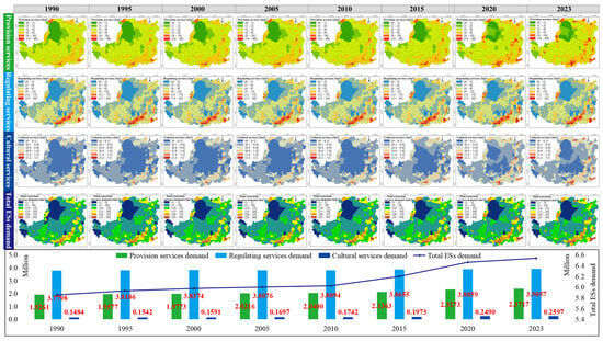
Figure 5.
Spatiotemporal maps showing the ESs demand of provision services, regulating services, cultural services, and total ESs in the LP from 1990 to 2023.
3.2. ESs Supply–Demand Relationship
3.2.1. Temporal Variations in ESSD
We aggregated the supply and demand values for the three ESs categories and total ESs across all counties on the LP for the eight periods to obtain the temporal characteristics of the ESs supply–demand matching status for the entire LP, as shown in Figure 6. It can be observed that the ESSD values for the three ESs categories and total ESs were consistently positive throughout the study period, indicating that all types of ESs and total ESs on the LP were in a supply-surplus state. Specifically, the supply of total ESs, provision services, and regulating services decreased while demand increased. Consequently, the surplus status of total ESs, provision, and regulating services overall showed a deteriorating trend. Although the supply of cultural services slightly increased, the surplus status also deteriorated due to a sharp increase in demand. Overall, the deterioration trend was greatest for cultural services, followed by provision services, and then regulating services, primarily related to the substantial increases in demand for cultural and provision services.

Figure 6.
The temporal trends of supply, demand, ESSD of provision services, regulating services, cultural services, and total ESs in the LP from 1990 to 2023 (ESSD: ESs supply–demand matching index).
3.2.2. Spatial Characteristics of ESSD
Figure 7 shows the spatial distribution and changes in ESSD for provision services, regulating services, cultural services, and total ESs on the LP from 1990 to 2023. For all ESs types, the ESSD of the vast majority of counties on the LP was positive (i.e., supply exceeds demand), especially for cultural services, which showed an almost universal positive state across the region. ESSD for provision services and total ESs showed negative values (i.e., demand exceeds supply) in scattered counties along the southeastern and northwestern borders of the LP. ESSD for regulating services showed concentrated contiguous negative characteristics in the Guanzhong Plain of the LP, with a few additional counties along the northwestern and northeastern borders also exhibiting supply deficits.

Figure 7.
Spatial distribution maps showing the ESSD of provision services, regulating services, cultural services, and total ESs in the LP from 1990 to 2023 (ESSD: ESs supply–demand matching index).
3.3. Drivers of ESs Supply–Demand Relationship
3.3.1. Detection of Key Influencing Factors via Geodetector
To better reveal the driving mechanisms behind changes in ESs supply–demand matching relationships on the LP, this study used the Geodetector model to explore the key influencing factors of ESSD. Based on the eleven latent drivers selected from different dimensions, the factor detection module of Geodetector was used to measure the influence intensity of these latent drivers on ESSD at the county scale. The results are shown in Table 3. It can be seen that the p values for all latent drivers were significant at the 0.001 level, indicating that the selected factors have sufficient explanatory power for ESSD on the LP. Ranking the explanatory power (q value) of the latent drivers on ESSD: COD > POP > GDP > FGD > SLO > ELE > RAI > TEM > EVA > FVC > FAD. Overall, COD had the strongest influence on ESSD, with a q value as high as 0.871. This was followed by POP, GDP, and FGD, with q values of 0.775, 0.763, and 0.753, respectively. The influence of other factors on ESSD was relatively weak. Therefore, COD, POP, GDP, and FGD are the main drivers influencing ESs supply–demand matching relationships on the LP.
Table 3.
The result of factor detector for ESSD in the LP.
3.3.2. Spatial Driving Intensity Analysis via GWR
This study further employed the GWR model to explore the spatial mechanisms of the impact of the four key drivers on ESs supply–demand matching relationships. When constructing the GWR model, we selected the Fixed gaussian function as the kernel function and used the Akaike information criterion to determine the optimal bandwidth. As shown in Figure 8a, regions with a deviance residual value between −2.5 and 2.5 almost occupied the entire study area, which indicates that the relationship between each of four drivers and the dependent variable is robust. In addition, the resulting goodness-of-fit R2 and adjusted R2 were 0.991 and 0.988, respectively, indicating that the constructed GWR model could explain over 98.8% of the variation in ESs supply–demand matching relationships. Figure 8 also shows the spatial differences in the influence of the four key drivers on ESs supply–demand matching relationships. The results showed that the local regression coefficients for FGD, POP, GDP, and COD varied among counties on the LP, fully reflecting the spatial heterogeneity of ESs supply–demand relationships of the LP. A positive regression coefficient indicates that an increase in the driver will improve the ESs supply–demand relationship, while a negative coefficient indicates that an increase in the driver will cause the ESs supply–demand relationship to deteriorate. Specifically, FGD exhibited a significant positive effect on ESSD across the LP during the study period. The influences of POP and GDP on ESSD exhibited a coexistence of positive promoting and negative inhibitory effects across the LP. COD primarily exerted a negative inhibitory effect on ESSD across the LP.

Figure 8.
Spatial distributions of impact coefficients for main influencing factors (FGD: proportion of forestland and grassland; POP: population density; GDP: GDP density; COD: proportion of construction land).
4. Discussion
4.1. Advantages and Uncertainties in Land-Cover-Based Approach
Quantifying ESs supply and ESs demand is an important aspect of ESs research [6,13]. Due to the issue of inconsistent dimensions between supply-side and demand-side assessments of ESs, it is difficult to achieve absolute supply–demand balance calculations, and the vast majority of studies can only achieve relative supply–demand balance measurements [9]. The land-cover-based ESs supply–demand quantitative matrix provides a unified and comparable measurement basis for supply and demand [28], thereby laying a methodological foundation for the systematic research of “quantitative assessment–characterization description–driver analysis–scenario simulation–regulation optimization” of absolute ESs supply–demand balance, and has been successfully applied in studies of many countries and regions [25,26,27,28,29,30]. It allows for rapid data acquisition, is highly adaptable, produces results with strong spatial visualization, and is suitable for regions of different scales, with data scarcity, and high complexity. It is also convenient to adjust ecosystem types, ESs classifications, and ESs supply–demand scores according to the specific study region [40]. Furthermore, although this method cannot fully depict the absolute levels of ESs supply and demand, it can fully represent the changing trends in ESs supply–demand relationships, thereby providing a certain scientific basis for alleviating regional ESs supply–demand contradictions.
Van Oudenhoven et al. [44] pointed out that indicators for evaluating ESs supply and demand must be quantifiable, sensitive to land use change, and scalable across spatial and temporal scales. However, quantifying human demand for ESs has become a challenge [9]. The ESs supply–demand quantitative matrix can meet the needs of current research to a certain extent. Nevertheless, this method highly depends on the experience, cognition, preferences, and attitudes of the experts surveyed, thus often possessing strong subjectivity and high uncertainty [28]. Although the scoring results for different ecosystem types in other countries or regions may differ from those for the LP, the relative rankings of ESs supply–demand scores among the three major land categories (construction land, agricultural land, ecological land) are relatively consistent, whether abroad, domestically, or on the LP. Additionally, we further measured the uncertainty level of the ESs supply–demand quantitative matrix adopted in this study using the sensitivity coefficient proposed in Section 2.3.2. The results are shown in Figure 9. The sensitivity coefficient for all land use types was less than 1, and even for many land use types, the sensitivity coefficient was far less than 1. This indicates that although the assignments in the quantitative matrix we adopted are empirical, the quantitative values in this study are reasonable, with low uncertainty.

Figure 9.
Sensitivity coefficient of different land use types (A1: paddy field; A2: arid land; B1: forestland; B2: shrub land; B3: wood land; B4: other forestlands; C1: highly covered grassland; C2: moderately covered grassland; C3: low covered grassland; D1: river and canals; D2: lakes; E1: bottom land; E2: swampland; F1: urban construction land; F2: rural settlements; F3: other construction land; G1: bare soil; G2: bare rock).
4.2. Key Factors Influencing ESs Supply–Demand Relationship
In this study, Geodetector and GWR models were used to capture the response characteristics of the dependent variable to the independent variables, including spatially non-stationary response characteristics. Our study indicates that ESs supply–demand matching relationships are closely related to topographic conditions (slope and elevation), climatic conditions (temperature, rainfall, and evapotranspiration), ecological restoration (foliage vegetation cover, proportion of farmland, and proportion of forestland and grassland), and socio-economic conditions (population density, GDP density, and proportion of construction land) (see Table 3). These results support and extend previous studies, demonstrating good explanatory power in selecting socio-ecological drivers to explain ESs supply–demand balance. Among all driving factors, the four factors, i.e., FGD, POP, GDP, and COD had much stronger influence intensities on ESs supply–demand matching relationships than other factors. This finding is similar to the results of Chen et al. [45] and Wen et al. [46]. Furthermore, we further discovered that the intensity and direction of the impact of these four factors on ESs supply–demand relationships exhibit significant spatial heterogeneity. This characteristic of spatially non-stationary responses of the dependent variable to the independent variables suggests that one-size-fits-all ESs management policies are difficult to apply universally. Interventions aimed at improving ESs supply–demand matching relationships may have little effect or even produce opposite effects in other areas.
Our results showed that COD had the highest influence (q = 0.871) and its regression coefficients were negative across the entire LP space, indicating that the expansion of construction land is the key driving force leading to the deterioration of the regional ESs supply–demand relationship (increased deficit risk or reduced surplus). This finding is consistent with the study of Dabasinskas and Sujetovienestudy [47]. The expansion of urbanization, industrial and mining development, and infrastructure construction directly encroaches on ecological lands like forestland and grassland that have high ESs supply potential (as shown in Figure 2, the ESs supply scores of these land types are much higher than construction land), causing “rigid” losses in supply capacity. On the other hand, the expansion of construction land is usually accompanied by population agglomeration and economic growth [48,49], further increasing regional demand for various ESs, creating a dual pressure of “decreasing supply–increasing demand”. Conversely, FGD exhibited significantly positive regression coefficients across the entire study area (i.e., increasing forest and grassland area helps improve supply–demand matching relationships). This result strongly validates the positive effects of long-term ecological projects implemented on the LP, such as the “Grain for Green Program” and “Natural Forest Protection Project” [50]. Forest and grass vegetation directly enhance the regional ESs supply capacity by strengthening key regulating services like water conservation, soil retention, and carbon sequestration. Our study revealed that the influences of POP and GDP on ESs supply–demand relationships exhibit more pronounced spatial heterogeneity, including reversals in the direction of influence. To some extent, this indicates the “dual effects” of population growth and economic development on ecosystems: while they can indeed impose pressure (even severe) on ecosystems [48,51], they may also allow more human resources, advanced technologies, and funds to be used for ecological management (e.g., ecological restoration projects, mine reclamation, pollution control) [9], thereby improving ecosystems. This phenomenon may be related to the existence of thresholds in the response of ESs to POP and GDP. This was also confirmed in the study of Peng et al. [52]. They found thresholds in the driving effects of population agglomeration and economic growth on ES, beyond which the direction of impact reversed. These findings once again strongly demonstrate that sustainable ESs management needs to consider the spatially differentiated intensity and nature of driving factors and implement more localized strategies.
4.3. Policy Implications
The findings regarding the key influence factors and their pronounced spatial heterogeneity on ESs supply–demand matching relationships within LP carry significant implications for regional land use planning and ecosystem management. These implications can be distilled into the following key recommendations:
- (1)
- Implementing strict spatial controls on construction land expansion. Our analysis unequivocally identifies COD as the factor exerting the strongest negative influence on ESs supply–demand balance across the entire LP. Construction expansion causes the loss of ecological lands while simultaneously driving increased ESs demand through associated population agglomeration and economic activity. Therefore, strictly controlling disorderly urban expansion, optimizing the spatial layout of construction land, and especially implementing strict development controls in ecologically sensitive areas and key areas for ESs supply, are crucial for maintaining regional ESs supply–demand balance.
- (2)
- Prioritizing continuous ecological restoration in high-demand or ecologically sensitive areas. The study demonstrates a consistent positive effect of FGD on improving ESs supply–demand relationships throughout the LP. However, there are also differences in the intensity of the positive effects of FGD, which indicates that its role in enhancing ESs supply and alleviating ESs supply–demand conflicts may be more critical in areas with fragile ecological foundations or where projects are intensively implemented. This further emphasizes the importance of continuous protection and restoration of forest–grass ecosystems in high-demand or ecologically sensitive areas.
- (3)
- Adopting spatially differentiated strategies for managing population and economic development pressures. Our analysis underscores the “dual effects” and potential threshold behaviors of socio-economic drivers. A uniform management approach is therefore inadequate. Policy interventions must be tailored based on local GWR results: (a) In spatial units where POP/GDP exert strong negative influences, strategies should focus on alleviating direct ecological burdens through stringent environmental regulations, resource efficiency promotion, pollution control, and potentially managing urban densification in sensitive fringes. (b) In spatial units where POP/GDP show positive influences, strategies should leverage available human and financial resources to actively channel efforts into ecological conservation, restoration projects, and fostering green economic development.
4.4. Limitations and Future Perspectives
This study also has some limitations that need to be pointed out, and further addressed in future research. First, similar to other studies, when constructing the ESSD to assess the ESs supply–demand relationship in this study, the spatial flow between ESs supply and demand cannot be reflected. Both the ESs supply and demand are fluid, and their flow processes are very complex [53]. However, due to the current lack of mature models for quantitatively characterizing the transfer process of ESs from supply areas to demand areas, particularly models for quantitatively simulating the flow paths, volumes, and consumption during flow, research on ESs supply–demand balance is limited. Furthermore, ESs can be generated at different spatiotemporal scales, and differences in ecological backgrounds and socio-economic conditions across scales can lead to variations in the types, capacity levels, and spatial characteristics of ESs supply and demand [21,48]. Future research could focus on multi-scale studies of supply–demand relationships and driving mechanisms to reveal scale effects and scale heterogeneity, which would help formulate more targeted and implementable regional ecosystem management strategies. Finally, comprehensive studies encompassing all types of ESs supply–demand face difficulties in identifying the dominant ESs supply–demand conflicts within a region. Future research could focus on the regional key ecological and environmental problems, selecting dominant ESs types for targeted studies to serve the practical needs of local ecological environment construction.
5. Conclusions
In this study, we employed a land-cover-based ESs supply–demand quantitative matrix to quantify and map ESs supply, demand, and their matching relationships on the LP from 1990 to 2023, and tested its rationality and reliability through sensitivity coefficients. We further focused on exploring key driving factors and the spatial non-stationarity of their impacts on ESs supply–demand relationships. Over the past three decades, although the overall ESs supply–demand matching on the LP remained in a supply-surplus state, the decrease in ESs supply and the increase in ESs demand led to a worsening trend in ESs supply–demand relationships towards deficit. Geodetector identified COD, POP, GDP, and FGD as key factors influencing changes in ESs supply–demand relationships, and their influence intensities exhibited spatial heterogeneity. COD had the strongest influence and exhibited a universally negative inhibitory effect on ESs supply–demand relationship changes, meaning that construction land expansion is the primary driver of the deterioration in ESs supply–demand relationships on the LP. FGD consistently exerted a significantly positive spatial effect on ESs supply–demand relationship changes, highlighting the critical role of vegetation restoration in improving ESs supply–demand relationships. The influences of POP and GDP exhibited a coexistence of positive promoting and negative inhibitory effects across space, indicating that the impacts of population growth and economic development on ESs have “dual effects” in the LP region. Overall, when formulating regional land use strategies and ecological management measures, the spatially differentiated intensity and direction of driving factors should be considered to achieve more localized sustainable management.
Author Contributions
Methodology, M.Y., M.W., L.C. and H.Z.; Software, M.Y.; Validation, H.N.; Formal analysis, M.W.; Investigation, M.Y., M.W., L.C. and H.N.; Writing—original draft, M.Y. and M.W.; Writing—review & editing, M.Y., M.W., L.C., H.Z. and H.N.; Project administration, L.C.; Funding acquisition, M.Y., L.C. and H.Z. All authors have read and agreed to the published version of the manuscript.
Funding
This work was jointly supported by the National Natural Science Foundation of China (42401384), the Humanities and Social Sciences Foundation of Ministry of Education of China (24YJCZH376), the Key Scientific Research Projects of Colleges and Universities in Henan Province (25A170008, 24B170003).
Data Availability Statement
The datasets that support the findings of this study are available from the corresponding author upon reasonable request.
Acknowledgments
The authors would like to thank the three anonymous reviewers for their helpful and constructive comments and suggestions which have substantially improved the quality of this manuscript.
Conflicts of Interest
The authors declare no conflict of interest.
References
- Costanza, R.; d’Arge, R.; de Groot, R.; Farber, S.; Grasso, M.; Hannon, B.; Limburg, K.; Naeem, S.; O’Neill, R.V.; Paruelo, J.; et al. The value of the world’s ecosystem services and natural capital. Nature 1997, 387, 253–260. [Google Scholar] [CrossRef]
- Ouyang, Z.; Zheng, H.; Xiao, Y.; Polasky, S.; Liu, J.; Xu, W.; Wang, Q.; Zhang, L.; Xiao, Y.; Rao, E.; et al. Improvements in ecosystem services from investments in natural capital. Science 2016, 352, 1455–1459. [Google Scholar] [CrossRef]
- Liu, Y.; Fu, B.; Wang, S.; Rhodes, J.R.; Li, Y.; Zhao, W.; Li, C.; Zhou, S.; Wang, C. Global assessment of nature’s contributions to people. Sci. Bull. 2023, 68, 424–435. [Google Scholar] [CrossRef] [PubMed]
- Ulrich, W.; Batáry, P.; Baudry, J.; Beaumelle, L.; Bucher, R.; Cerevková, A.; de la Riva, E.G.; Felipe-Lucia, M.R.; Gallé, R.; Kesse-Guyot, E.; et al. From biodiversity to health: Quantifying the impact of diverse ecosystems on human well-being. People Nat. 2023, 5, 69–83. [Google Scholar] [CrossRef]
- De Knegt, B.; Lof, M.E.; Le Clec’h, S.; Alkemade, R. Growing mismatches of supply and demand of ecosystem services in the Netherlands. J. Environ. Manag. 2025, 373, 123442. [Google Scholar] [CrossRef]
- Ding, H.; Sun, R. Supply-demand analysis of ecosystem services based on socioeconomic and climate scenarios in North China. Ecol. Indic. 2023, 146, 109906. [Google Scholar] [CrossRef]
- Elliot, T.; Goldstein, B.; Gomez-Baggethun, E.; Proenca, V.; Rugani, B. Ecosystem service deficits of European cities. Sci. Total Eviron. 2022, 837, 155875. [Google Scholar] [CrossRef] [PubMed]
- Sitotaw, T.M.; Willemen, L.; Meshesha, D.T.; Weldemichael, M.; Nelson, A. Modelling the impact of ecosystem fragmentation on ecosystem services in the degraded Ethiopian highlands. Ecol. Inform. 2025, 87, 103100. [Google Scholar] [CrossRef]
- Yang, M.; Zhao, X.; Wu, P.; Hu, P.; Gao, X. Quantification and spatially explicit driving forces of the incoordination between ecosystem service supply and social demand at a regional scale. Ecol. Indic. 2022, 137, 108764. [Google Scholar] [CrossRef]
- Millennium Ecosystem Assessment (MA). Ecosystems and Human Well-Being; Island Press: Washington, DC, USA, 2005. [Google Scholar]
- IPBES. Summary for Policymakers of the Global Assessment Report on Biodiversity and Ecosystem Services of the Intergovernmental Science-Policy Platform on Biodiversity and Ecosystem Services. 2019. Available online: https://www.ipbes.net/system/tdf/spm_global_unedited_advance.pdf?file=1&type=node&id=35245 (accessed on 12 March 2025).
- Wood, S.L.R.; Jones, S.K.; Johnson, J.A.; Brauman, K.A.; Chaplin-Kramer, R.; Fremier, A.; Girvetz, E.; Gordon, L.J.; Kappel, C.V.; Mandle, L.; et al. Distilling the role of ecosystem services in the Sustainable Development Goals. Ecosyst. Serv. 2018, 29, 70–82. [Google Scholar] [CrossRef]
- Zhang, J.; Wang, M.; Liu, K.; Chen, S.; Zhao, Z. Social-ecological system sustainability in China from the perspective of supply-demand balance for ecosystem services. J. Clean. Prod. 2025, 497, 145039. [Google Scholar] [CrossRef]
- De Groot, R.S.; Alkemade, R.; Braat, L.; Hein, L.; Willemen, L. Challenges in integrating the concept of ecosystem services and values in landscape planning, management and decision making. Ecol. Complex. 2010, 7, 260–272. [Google Scholar] [CrossRef]
- Casado-Arzuaga, I.; Madariaga, I.; Onaindia, M. Perception, demand and user contribution to ecosystem services in the Bilbao Metropolitan Greenbelt. J. Environ. Manag. 2013, 129, 33–43. [Google Scholar] [CrossRef]
- Bennett, D.E.; Gosnell, H. Integrating multiple perspectives on payments for ecosystem services through a social-ecological systems framework. Ecol. Econ. 2015, 116, 172–181. [Google Scholar] [CrossRef]
- Qu, Q.; Zhang, K.; Niu, J.; Xiao, C.; Sun, Y. Spatial-Temporal Differentiation of Ecosystem Service Trade-Offs and Synergies in the Taihang Mountains, China. Land 2025, 14, 513. [Google Scholar] [CrossRef]
- Huang, Z.; Wang, X.; Yuan, M.; Duan, W.; Xia, J.; Li, J.; Zhao, Y. Differential Response of Ecosystem Service to Restoration Methods and Restoration Time in Shallow Landslide-Prone Areas. Land Degrad. Dev. 2025, 36, 3051–3062. [Google Scholar] [CrossRef]
- Lu, Z.; Li, W.; Yue, R. Investigation of the long-term supply-demand relationships of ecosystem services at multiple scales under SSP-RCP scenarios to promote ecological sustainability in China’s largest city cluster. Sustain. Cities Soc. 2024, 104, 105295. [Google Scholar] [CrossRef]
- Yang, M.; Gao, X.; Zhao, X.; Wu, P. Scale effect and spatially explicit drivers of interactions between ecosystem services—A case study from the Loess Plateau. Sci. Total Environ. 2021, 785, 147389. [Google Scholar] [CrossRef]
- Cui, F.; Tang, H.; Zhang, Q.; Wang, B.; Dai, L. Integrating ecosystem services supply and demand into optimized management at different scales: A case study in Hulunbuir, China. Ecosyst. Serv. 2019, 39, 100984. [Google Scholar] [CrossRef]
- Liu, Y.; Yu, D.; Fu, B.; Cao, M.; Chen, J. Research progress on the biodiversity and ecosystem service scenario simulations. Acta Ecol. Sin. 2020, 40, 5863–5873. (In Chinese) [Google Scholar] [CrossRef]
- Shi, R.; Huang, X.; Wang, L.; Xiang, Y.; Huang, C. Land Use Changes and Sustainable Development Goals Alignment Through Assessing Ecosystem Service Supply and Demand Balance. Land Degrad. Dev. 2025, 36, 2651–2665. [Google Scholar] [CrossRef]
- Kandziora, M.; Burkhard, B.; Müller, F. Mapping Provisioning Ecosystem Services at the Local Scale Using Data of Varying Spatial and Temporal Resolution. Ecosyst. Serv. 2013, 4, 47–59. [Google Scholar] [CrossRef]
- Kaiser, G.; Burkhard, B.; Römer, H.; Sangkaew, S.; Graterol, R.; Haitook, T.; Sterr, H.; Sakuna-Schwartz, D. Mapping Tsunami Impacts on Land Cover and Related Ecosystem Service Supply in Phang Nga, Thailand. Nat. Hazard. Earth Sys. 2013, 13, 3095–3111. [Google Scholar] [CrossRef]
- Vihervaara, P.; Kumpula, T.; Tanskanen, A.; Burkhard, B. Ecosystem Services: A Tool for Sustainable Management of Human Environment Systems: Case Study Finnish Forest Lapland. Ecol. Complex. 2010, 7, 410–420. [Google Scholar] [CrossRef]
- Burkhard, B.; Müller, A.; Müller, F.; Grescho, V.; Anh, Q.; Arida, G.; Bustamante, J.V.; Chien, H.V.; Heong, K.L.; Escalada, M.; et al. Land Cover Based Ecosystem Service Assessment of Irrigated Rice Cropping Systems with Different Production Intensities in Southeast Asia: An Explorative Study. Ecosyst. Serv. 2015, 14, 76–87. [Google Scholar] [CrossRef]
- Lyu, Y.; Sheng, L.; Wu, C. Improving land-cover-based expert matrices to quantify the dynamics of ecosystem service supply, demand, and budget: Optimization of weight distribution. Ecol. Indic. 2023, 154, 110515. [Google Scholar] [CrossRef]
- Chen, W.; Chi, G. Spatial mismatch of ecosystem service demands and supplies in China, 2000–2020. Environ. Monit. Assess. 2022, 194, 295. [Google Scholar] [CrossRef]
- Zhang, Z.; Fang, F.; Yao, Y.; Ji, Q.; Cheng, X. Exploring the Response of Ecosystem Services to Socioecological Factors in the Yangtze River Economic Belt, China. Land 2024, 13, 728. [Google Scholar] [CrossRef]
- González-García, A.; Palomo, I.; González, J.A.; López, C.A.; Montes, C. Quantifying spatial supply-demand mismatches in ecosystem services provides insights for land-use planning. Land Use Policy 2020, 94, 104493. [Google Scholar] [CrossRef]
- Mashizi, A.K.; Sharafatmandrad, M. Investigating tradeoffs between supply, use and demand of ecosystem services and their effective drivers for sustainable environmental management. J. Environ. Manag. 2021, 289, 112534. [Google Scholar] [CrossRef]
- Wang, S.; Fu, B.; Wu, X.; Wang, Y. Dynamics and sustainability of social-ecological systems in the Loess Plateau. Resour. Sci. 2020, 42, 96–103. (In Chinese) [Google Scholar] [CrossRef]
- Fu, B.; Liu, Y.; Cao, Z.; Wang, Z.; Wu, X. Current conditions, issues, and suggestions for ecological protection and high-quality development in Loess Plateau. Bull. Chin. Acad. Sci. 2023, 38, 1110–1117. (In Chinese) [Google Scholar]
- Wang, X.; Peng, S.; Wu, J.; Zheng, K.; Wang, S.; Shangguan, Z.; Deng, L. Simulation of the Key Ecosystem Services Changes in China’s Loess Plateau under Various Shared Socioeconomic Pathways Scenarios. Ecosyst. Health Sustain. 2024, 10, 0200. [Google Scholar] [CrossRef]
- Yang, Q.; Qian, H.; Gao, Y.; Duan, Y.; Cao, Z.; Tian, P.; Li, K.; Yang, S.; Zhao, W.; Long, Q. Spatio-temporal evolution and driving mechanism of ecosystem services in typical hilly and gully areas of the loess Plateau: A case study in Yan’an Region, Shaanxi Province. Ecol. Indic. 2025, 177, 113773. [Google Scholar] [CrossRef]
- Fu, B.; Wang, S.; Liu, Y.; Liu, J.; Liang, W.; Miao, C. Hydrogeomorphic Ecosystem Responses to Natural and Anthropogenic Changes in the Loess Plateau of China. Annu. Rev. Earth Planet. Sci. 2017, 45, 223–243. [Google Scholar] [CrossRef]
- Burkhard, B.; Kroll, F.; Nedkov, S.; Müller, F. Mapping ecosystem service supply, demand and budgets. Ecol. Indic. 2012, 21, 17–29. [Google Scholar] [CrossRef]
- Jiang, C.; Yang, Z.; Wen, M.; Huang, L.; Liu, H.; Wang, J.; Chen, W.; Zhuang, C. Identifying the spatial disparities and determinants of ecosystem service balance and their implications on land use optimization. Sci. Total Environ. 2021, 793, 148472. [Google Scholar] [CrossRef]
- Wu, X.; Liu, S.; Zhao, S.; Hou, X.; Xu, J.; Dong, S.; Liu, G. Quantification and driving force analysis of ecosystem services supply, demand and balance in China. Sci. Total Environ. 2019, 652, 1375–1386. [Google Scholar] [CrossRef]
- Zhai, T.; Ma, Y.; Huang, L.; Lu, Y.; Li, L.; Chen, Y.; Chang, M.; Ma, Z. Research on the spatiotemporal evolution characteristics and driving mechanisms of supply-demand risks of ecosystem services in the yellow river basin integrating the hierarchy of needs theory. Ecol. Indic. 2025, 171, 113229. [Google Scholar] [CrossRef]
- Wang, J.; Xu, C. Geodetector: Principle and prospective. Acta Geogr. Sin. 2017, 72, 116–134. (In Chinese) [Google Scholar]
- Li, K.; Fan, H.; Ouyang, J.; Yao, P. Valuation of the 2020 gross ecosystem product of China and analysis of driving factors. J. Clean. Prod. 2025, 513, 145741. [Google Scholar] [CrossRef]
- Van Oudenhoven, A.P.E.; Petz, K.; Alkemade, R.; Hein, L.; de Groot, R.S. Framework for systematic indicator selection to assess effects of land management on ecosystem services. Ecol. Indic. 2012, 21, 110–122. [Google Scholar] [CrossRef]
- Chen, Y.; Qiao, X.; Yang, Y.; Zheng, J.; Dai, Y.; Zhang, J. Identifying the spatial relationships and drivers of ecosystem service supply-demand—Demand matching: A case of Yiluo River Basin. Ecol. Indic. 2024, 163, 112122. [Google Scholar] [CrossRef]
- Wen, Y.; Li, M.; Chen, Z.; Li, W. Changes in ecosystem services supply-demand and key drivers in Jiangsu Province, China, from 2000 to 2020. Land Degrad. Dev. 2024, 35, 4666–4681. [Google Scholar] [CrossRef]
- Dabasinskas, G.; Sujetoviene, G. Spatial and Temporal Changes in Supply and Demand for Ecosystem Services in Response to Urbanization: A Case Study in Vilnius, Lithuania. Land 2024, 13, 4. [Google Scholar] [CrossRef]
- Deng, L.; Yang, J.; Yin, X.; Jia, K.; Sun, J.; Shu, S.; Huang, A. Supply and demand of ecosystem services and its multi-spatial scale response to urbanization in Guangdong-Hong Kong-Macao Greater Bay Area. Acta Ecol. Sin. 2024, 44, 9094–9107. (In Chinese) [Google Scholar]
- Zhu, Z.; Fu, W.; Liu, Q. Correlation between urbanization and ecosystem services in Xiamen, China. Environ. Dev. Sustain. 2021, 23, 101–121. [Google Scholar] [CrossRef]
- Wu, X.; Wang, S.; Fu, B.; Feng, X.; Chen, Y. Socio-ecological changes on the Loess Plateau of China after Grain to Green Program. Sci. Total Environ. 2019, 678, 565–573. [Google Scholar] [CrossRef]
- Mehring, M.; Ott, E.; Hummel, D. Ecosystem services supply and demand assessment: Why social-ecological dynamics matter. Ecosyst. Serv. 2018, 30, 124–125. [Google Scholar] [CrossRef]
- Peng, J.; Tian, L.; Liu, Y.; Zhao, M.; Hu, Y.; Wu, J. Ecosystem services response to urbanization in metropolitan areas: Thresholds identification. Sci. Total Environ. 2017, 607, 706–714. [Google Scholar] [CrossRef]
- Qu, C.; Xu, J.; Li, W.; Zhai, Y.; Wang, Y.; Liu, B.; Yan, S. Integrating circuit theory and network modeling to identify ecosystem carbon sequestration service flow networks. Ecol. Inform. 2025, 87, 103077. [Google Scholar] [CrossRef]


Disclaimer/Publisher’s Note: The statements, opinions and data contained in all publications are solely those of the individual author(s) and contributor(s) and not of MDPI and/or the editor(s). MDPI and/or the editor(s) disclaim responsibility for any injury to people or property resulting from any ideas, methods, instructions or products referred to in the content. |
© 2025 by the authors. Licensee MDPI, Basel, Switzerland. This article is an open access article distributed under the terms and conditions of the Creative Commons Attribution (CC BY) license (https://creativecommons.org/licenses/by/4.0/).