Article

Spatio-Temporal Evolution and Driving Factors of Eco-Environmental Response to Land Use Transformation in China’s Southern Hilly Area During 2000–2020

1
Institute of Rural Development, Zhejiang Academy of Agricultural Sciences, Hangzhou 310021, China
2
New Quality Productive Forces Think Tank, Zhejiang Academy of Agricultural Sciences, Hangzhou 310021, China
3
School of Public Affairs, Zhejiang Gongshang University, Hangzhou 310018, China
*
Author to whom correspondence should be addressed.
Land 2025, 14(9), 1766; https://doi.org/10.3390/land14091766
Submission received: 5 August 2025 / Revised: 28 August 2025 / Accepted: 29 August 2025 / Published: 30 August 2025
(This article belongs to the Special Issue Landscape Ecological Risk in Mountain Areas)

Abstract

Hilly areas serve as critical ecological barriers yet face developmental challenges, drawing increasing attention to how land use transformation affects eco-environmental quality (EEQ). Systematic studies on EEQ drivers in complex terrains remain limited, particularly regarding nonlinear and interactive effects. This study examines Zhejiang’s hilly area—typical of southern China’s hills—using land use data from 2000, 2010, and 2020. Methods including land use transfer matrix, EEQI, hotspot analysis, and XGBoost-SHAP were applied to assess impacts and quantify drivers. Results show a slight but consistent decline in EEQ index (EEQI) (0.7635 to 0.7472), driven primarily by rapid built-up land (BL) expansion (276.41% increase). NDVI was the most influential factor (SHAP: 0.1226, >59%), followed by GDP per unit area and temperature. NDVI showed a threshold effect (>0.65 strengthens benefit), and strong interaction with per capita GDP. A slope-vegetation coupling mechanism was identified: on slopes > 30°, high NDVI significantly amplifies EEQ improvement, highlighting the importance of vegetation conservation on steep slopes. These findings provide a scientific basis for targeted land management in hilly regions of southern China and similar areas.

1. Introduction

Since the 21st century, China’s territorial spatial pattern has undergone profound restructuring under the dual objectives of rapid urbanization and ecological protection [1,2]. This process encompasses changes in land use types, structural adjustments, and multidimensional spatial reorganization [3,4]. Against the backdrop of ecological civilization construction being elevated to a national strategy in China, territorial spatial transformation has emerged as a core pathway for harmonizing human-land relationships and optimizing spatial structures [5]. As a critical indicator for assessing regional sustainable development levels, EEQ exhibits dynamic changes closely linked to land use patterns [6].
Significant scholarly achievements have accumulated regarding the eco-environmental effects of land use transformation, primarily concentrating on the development of EEQ evaluation methods, quantitative analyses of the impacts of land use transformation on EEQ, and investigations into spatial heterogeneity [7,8,9]. Commonly employed methodologies include the land use transfer matrix, ecological environment quality index (EEQI), ecosystem service value assessment models, and landscape pattern analysis [10,11,12]. Research indicates that early urban expansion often induced localized ecological degradation. However, following the advancement of China’s ecological civilization strategy, numerous regions have shifted towards quality-enhancing development models, resulting in a deceleration or even reversal of negative EEQ trends [13]. Spatially, pronounced ecological pressures are evident in the urbanized eastern coastal regions of China, whereas conditions in ecologically fragile central-western areas have improved due to policy interventions such as the Grain for Green Program [14,15,16]. Nevertheless, extensive research has focused on national, provincial, or plain/arid region scales, while systematic research targeting China’s southern hilly area remains relatively scarce. This region features fragmented terrain, diverse ecosystems, and a sensitive human-land relationship, resulting in a potential EEQ response mechanism that may significantly differ from other areas.
EEQ dynamics are co-driven by multiple factors, encompassing natural conditions and socioeconomic development [17]. Among these, natural elements such as topography and climate define the baseline conditions and sensitivity of regional ecosystems. Socioeconomic factors, including population density and GDP growth, influence ecological environment quality both directly and indirectly through land use transformation [18,19]. In recent years, scholars have widely adopted multiple regression models, geographical detector models, geographically weighted regression (GWR), structural equation modeling (SEM), and machine learning approaches to identify and quantify the influence and underlying mechanisms of various drivers on EEQ [20,21]. However, these approaches typically exhibit certain limitations: (1) They often struggle to effectively capture complex nonlinear relationships among variables, leading to an insufficiently profound understanding of driving mechanisms; (2) Analyses of interactions between driving factors remain relatively inadequate; (3) While capable of handling complex relationships, the “black-box” nature of machine learning methods poses challenges to model interpretability. A novel framework synergistically integrating XGBoost (for elucidating nonlinear relationships) and the SHAP explainer method (addressing “black-box” interpretability issues, quantifying importance, and revealing interactions) can circumvent these limitations, enabling the identification and quantification of key drivers influencing EEQ.
Although some studies have focused on the eco-environmental response mechanisms in the eastern plains of China, relatively less attention has been paid to the hilly regions in the south [22]. The eastern plains, characterized by gentle terrain and relatively homogeneous spatial factors, exhibit spatial agglomeration patterns dominated primarily by a single gradient of development intensity. In contrast, the hilly areas of southern China are marked by high topographic fragmentation, significant slope variability, rich biodiversity, high erosion sensitivity, and notable topographic constraints on construction activities. The superposition of vertical gradients along terrain features and horizontal gradients of urbanization has led to systematic differences in how EEQ responds to land use transformation compared to the eastern plains. However, there remains a lack of systematic research on the response of EEQ and its driving factors within complex hilly terrains, particularly regarding nonlinear influences and interaction effects.
The hilly area of Zhejiang serves as an ideal window for observing the complexity of eco-environmental responses. Since the implementation of the “Thousand Village Demonstration, Ten Thousand Village Improvement” project in 2003, Zhejiang has achieved remarkable success in integrating village restructuring, ecological restoration, and high-quality development, establishing itself as a national model [23]. Conducting a systematic study on the relationship between land use transformation and EEQ in the hilly area of Zhejiang as a typical case will not only help reveal the ecological effects of land use changes in complex geographical settings but also provide valuable insights and references for other hilly area in southern China.
Building upon this foundation, the hilly area of Zhejiang Province were selected as the study area. Land use data from 2000, 2010, and 2020 were utilized, and methods including the land use transfer matrix, EEQI, hotspot analysis, and other spatial analysis techniques were employed to reveal the response of EEQ to territorial spatial transformation. The XGBoost-SHAP method was innovatively introduced to analyze the nonlinear influences of driving factors. This study was designed to: (1) systematically examine the spatiotemporal response of EEQ to land use changes in hilly area; (2) quantitatively evaluate the relative importance of various driving factors, identify thresholds of their nonlinear effects, and quantify interaction effects between key factors by integrating the XGBoost machine learning model with the SHAP interpretability framework. The limitations of traditional linear models in capturing complex relationships were overcome through this methodology, which represents the core innovation of this research.

2. Materials and Methods

2.1. Overview of the Study Area

China’s southern hilly area represents a globally significant ecological region characterized by its vast coverage of subtropical evergreen broad-leaved forests, which play a crucial role in carbon sequestration, biodiversity conservation, and water regulation. This region is typified by complex topography and long-standing human-land interactions. Focusing on this broader context, this study selects the hilly area of Zhejiang Province as a representative case. Zhejiang, located on China’s southeastern coast, lies within the subtropical monsoon climate zone and is characterized predominantly by hilly terrain. The study area comprises 26 hilly counties, covering the entire prefectures of Lishui and Quzhou, as well as parts of Hangzhou, Wenzhou, Jinhua, and Taizhou. This region exemplifies the low-relief hilly landscapes typical of southern China (Figure 1) and represents a core implementation zone of Zhejiang’s “Thousand-Village Demonstration, Ten-Thousand-Village Renovation” project and rural revitalization strategy.
The area possesses a sound ecological foundation, with forest coverage generally exceeding 70% and abundant water resources. However, it also exhibits relatively high ecological vulnerability and is particularly sensitive to land use changes. Over the past two decades, driven by ecological civilization strategies and continuous rural policy implementation, the region has undergone significant land use transformation. This includes the consolidation and optimization of rural residential areas, spatial restructuring of built-up land, and shifts in agricultural land use types. These changes have profoundly influenced both socioeconomic development and EEQ.
The period from 2000 to 2020 was selected to cover the critical phase of ecological restoration policies and investigate the medium—to long-term impacts of land use transformation.

2.2. Data Sources

Land use data (2000, 2010, 2020; spatial resolution: 30 m × 30 m) [24] and GDP per unit area data (spatial resolution: 1 km × 1 km) [25] were obtained from the Data Center for Resources and Environmental Sciences, Chinese Academy of Sciences (https://www.resdc.cn/, accessed on 10 April 2023 and 21 April 2025). DEM data (spatial resolution: 30 m × 30 m) were acquired from the Geospatial Data Cloud (http://www.gscloud.cn/, accessed on 18 April 2025). Temperature data (spatial resolution: 1 km × 1 km) were sourced from the National Tibetan Plateau/Third Pole Environment Data Center (http://data.tpdc.ac.cn, accessed on 18 April 2025) [26]. NDVI data (spatial resolution: 1 km × 1 km) were downloaded from NASA’s EarthData portal (https://www.earthdata.nasa.gov/, accessed on 5 August 2024) [27]. Population density data (spatial resolution: 1 km × 1 km) were provided by WorldPop (https://www.worldpop.org/, accessed on 21 April 2025). Following established methodologies [28] and considering regional characteristics, land use types were classified into six categories: Cropland (CL), Forestland (FL), Grassland (GL), Water Bodies (WB), Built-up Land (BL), and Unused Land (UL). All datasets were uniformly reprojected to the “WGS_1984” coordinate system and resampled to a 1km grid resolution.

2.3. Methods

2.3.1. Land Use Transformation

(1)
Land Use Transfer Matrix
Land Use Transfer Matrix is a widely employed quantitative analytical tool for identifying mutual transformation relationships and intensities between different land use categories [29]. This method uses a two-dimensional matrix to capture land use gains and losses, revealing dynamic change processes. Specifically, the rows represent land use types in the initial year, the columns represent land use categories in the terminal year, and each element within the matrix quantifies the area transitioning from one land use category to another. This method enables the identification of dominant land use transformation directions, key categories experiencing net loss or gain, and provides foundational data for supporting subsequent eco-environmental impact assessments. Its mathematical expression is given by:
s i j = s 11 s 12 s 1 n s 21 s 22 s 2 n s n 1 s n 2 s n n
where n denotes the total number of land use categories in the study area, and sij represents the area converted from category i to category j during the study period.
(2)
Gravity Model
The gravity center model is a widely applied spatial analysis technique that integrates temporal and spatial information to visually represent the dynamic evolution of regional elements [30,31]. In this study, the gravity center model was employed to compare the coordinates of the gravity centers for each land use category at the three time points, thereby determining the spatial expansion direction and migration velocity of land use changes. Its calculation formula is expressed as follows:
x ¯ = i = 1 n M t i x i i = 1 n M t i , y ¯ = i = 1 n M t i y i i = 1 n M t i
where x ¯ and y ¯ denote the longitude and latitude coordinates, respectively, of the geographic gravity center for a specific land use category in year t; n represents the total number of spatial units; x i and y i are the geometric center coordinates of the i-th spatial unit; and Mti signifies the attribute value (e.g., area) of the land use category within the i-th spatial unit in year t.
(3)
Standard Deviational Ellipse (SDE)
SDE method is a spatial econometric analysis technique capable of revealing the overall morphological characteristics of spatial element distributions [32,33]. This method generates an elliptical shape by calculating the projections of the standard deviations of a land use type’s spatial distribution onto its major and minor axes. It provides a visual representation of the directional trend and concentration level of the land use distribution [34]. The relevant formulas are:
tan θ = i = 1 n x i ¯ 2 i = 1 n y i ¯ 2 + i = 1 n x i ¯ 2 i = 1 n y i ¯ 2 2 + 4 i = 1 n x i ¯ y i ¯ 2 2 i = 1 n x i ¯ y i ¯
σ x = i = 1 n x i ¯ cos θ y i ¯ sin θ 2 n , σ y = i = 1 n x i ¯ sin θ y i ¯ cos θ 2 n
The center of the SDE corresponds to the geographic gravity center of a specific land use category. The rotation angle of the ellipse, denoted by θ, represents the clockwise angle between true north and the major axis and is derived from Equation (3). The semi-axis lengths of the SDE, σ x and σ y , are calculated using Equation (4). The direction of the major axis indicates the orientation of greater dispersion, while the minor axis indicates the direction of higher aggregation. Consequently, an elongated ellipse signifies a discrete distribution of the land use category. Conversely, an ellipse approaching a circular shape indicates minimal difference between the lengths of the major and minor axes and reflects a more concentrated distribution.

2.3.2. Eco-Environmental Response

(1)
EEQI
EEQI is a land-use-classification-based metric widely applied for assessing regional EEQ [35]. It primarily reflects the EEQ during a specific period by integrating the EEQ value of each land use category and its proportional area [36]. This indicator not only considers the functional differences in various land use types within ecosystems but also captures the comprehensive impact of structural changes in land use on the eco-environment. The formula is expressed as:
E V t = i = 1 n A k i R i T A
where EVt denotes the EEQI value in year t, Ri represents the EEQI weight assigned to the i-th land use category (Table 1, values referenced from [9]), n signifies the total number of land use categories, Aki indicates the area of the i-th land use category, and TA is the total area. In this study, the EEQI classification was established using the natural breaks (Jenks) method in ArcGIS 10.8, supplemented by relevant literature [15]. The index values were categorized into five levels: lowest (0 ≤ EEQI < 0.2), low (0.2 ≤ EEQI < 0.5), moderate (0.5 ≤ EEQI < 0.7), good (0.7 ≤ EEQI < 0.85), and excellent (0.85 ≤ EEQI ≤ 1.00).
(2)
Hot spot analysis
Hot spot analysis, based on the Getis-Ord Gi* statistic, is a spatial statistical method used to identify statistically significant spatial clusters of high values (hot spots) or low values (cold spots) within a dataset [37]. Its fundamental principle involves calculating the correlation between the attribute value of each spatial unit and the values within its neighborhood to determine whether it is significantly higher or lower than the surrounding area [38]. In this study, hot spot areas typically represent regions with notable ecological environment improvement, while cold spot areas potentially face ecological degradation risks. This method facilitates the identification of spatial heterogeneity in eco-environmental responses. The formula is expressed as:
G i * = j = 1 n W i j Y j / j = 1 n Y j
where Gi* denotes the hot spot statistic for spatial unit i, Yj represents the attribute value at spatial unit j, Wij is the spatial weight matrix defining the relationship between units i and j, and n signifies the total number of spatial units. A significantly positive Gi* value (Gi* > 0) indicates a hot spot, while a significantly negative value (Gi* < 0) identifies a cold spot. This study employed the Getis-Ord Gi* tool in ArcGIS 10.8 to perform hotspot analysis. The spatial relationship was determined using the fixed distance band method, with Euclidean distance selected as the distance method. Clusters with p-values < 0.1, <0.05, and <0.01 were identified as having 90%, 95%, and 99% confidence levels, respectively.

2.3.3. Driving Factors

(1)
Driving factors selection
Changes in EEQ are influenced by numerous factors. Based on relevant studies [39,40] and the specific context of the study area, natural factors and social factors were selected as the two primary categories of explanatory variables. To avoid multicollinearity among multiple explanatory variables [41,42], eight potential driving factors were chosen and tested for variance inflation factor (VIF) using SPSS 26. The results indicated that all VIF values were below 5, confirming the absence of multicollinearity, as presented in Table 2.
(2)
XGBoost
XGBoost is an ensemble learning algorithm based on decision trees. This method iteratively trains multiple Classification and Regression Trees (CART), adjusting weights based on residuals in each iteration to minimize the loss function [43]. Compared to traditional machine learning algorithms, XGBoost significantly enhances training and prediction speeds through algorithmic optimization and parallel processing. It offers advantages in efficiency, accuracy, and the capability to model complex nonlinear relationships [44], and is widely applied in fields such as environmental science, remote sensing monitoring, and land use change studies [45]. The objective function is expressed as:
O b j θ = i = 1 n L y i , y ^ i + k = 1 K Ω f k
where O b j θ denotes the objective function, L y i , y ^ i represents the loss function between predicted values and true values, Ω f k is the regularization term that controls model complexity to prevent overfitting, and fk signifies the output function of the k-th decision tree. The machine learning modeling and interpretation were conducted in Python 3.13. The XGBoost algorithm was implemented using the xgboost library.
(3)
SHAP
The SHAP interpretability model originates from the concept of Shapley values in cooperative game theory. SHAP assigns each feature a contribution score, known as the SHAP value, to quantify its impact on the model’s output [46]. This model can further decompose each feature’s contribution into its main effect and interaction effects, establishing SHAP as a universal framework for interpreting diverse algorithms [47]. This study employs the SHAP method to measure the relative importance of driving factors, their partial dependence relationships, and interaction effects. The SHAP values were calculated using the shap library.

3. Results

3.1. Spatio-Temporal Evolution of Land Use Transformation

3.1.1. Changes in Land Use in Study Area

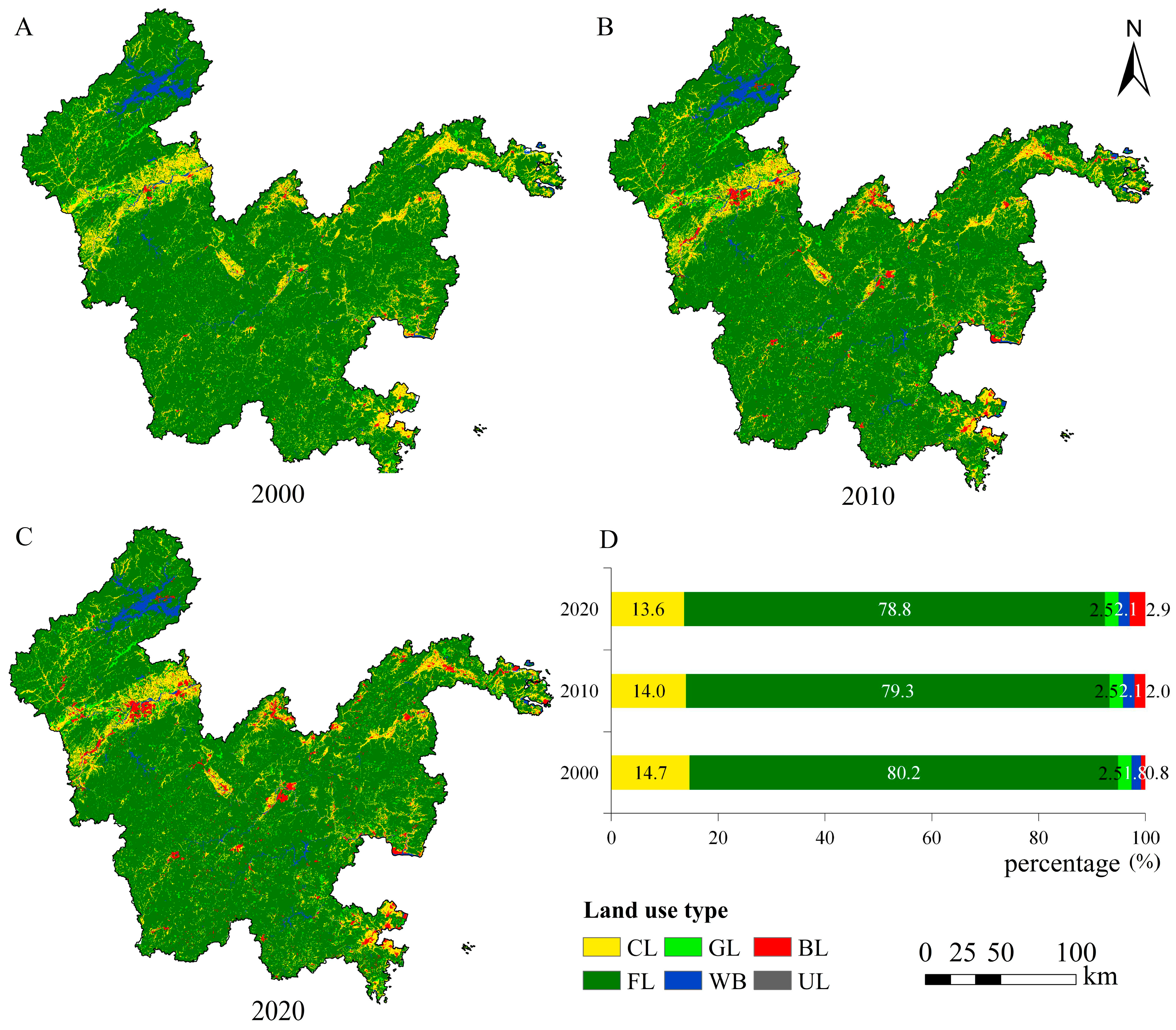
The two predominant land use categories within the study area were FL and CL, collectively accounting for between 92.42% and 94.85% of the total area. FL experienced the largest decline, decreasing by 617.76 km2. This was followed by CL, which decreased by 462.87 km2. The proportions of GL and UL remained stable at 2.5% and 0.05%, respectively. WB area increased by 124.89 km2, a growth of 15.10%. BL area expanded rapidly, increasing by 967.12 km2, with a growth rate of 276.41%. Regarding phased changes, all six land use categories showed notably greater change magnitudes during 2000–2010 compared to 2010–2020 (Figure 2).

3.1.2. Characteristics of Land Use Transformation

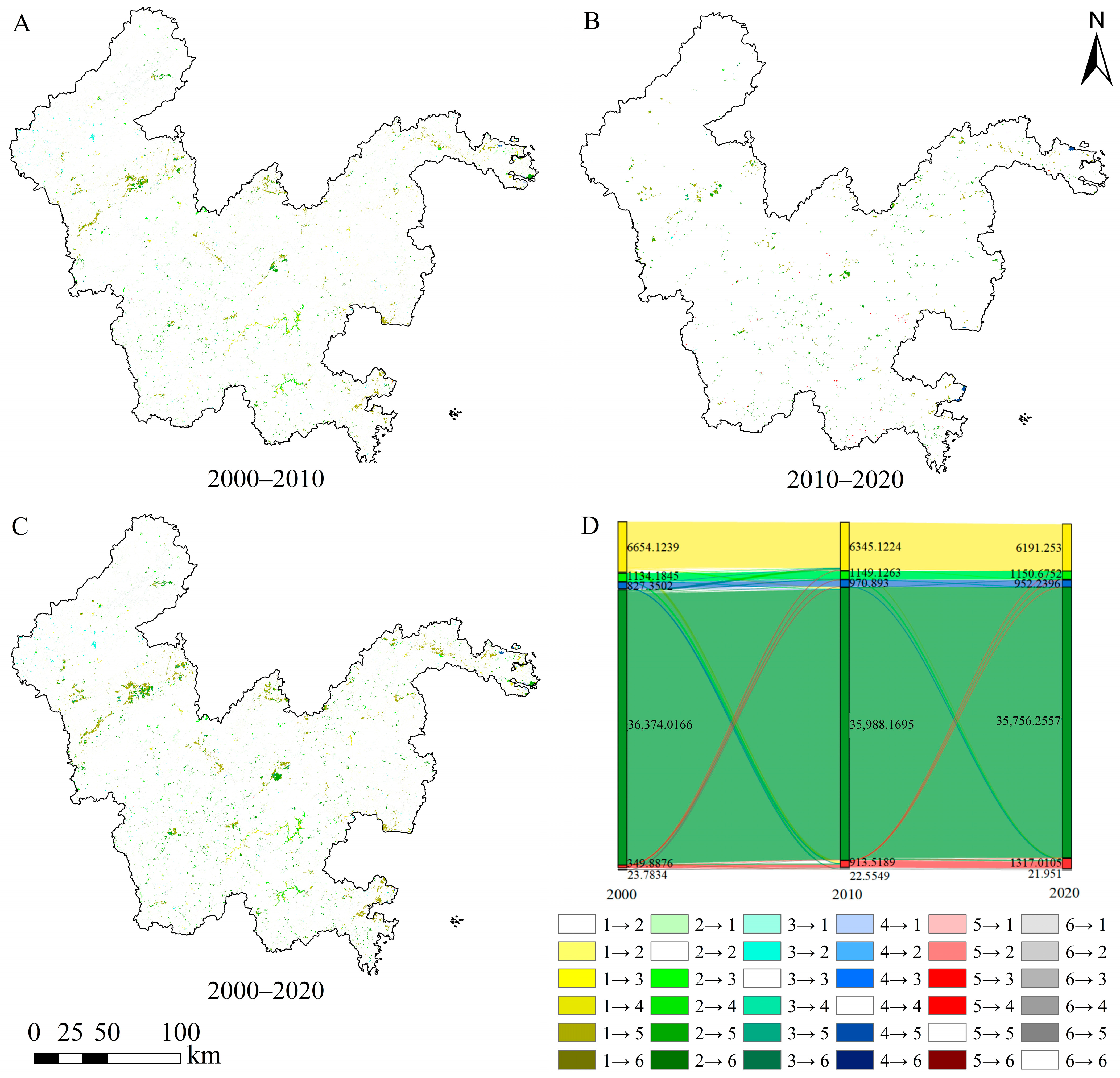
A total of 1815.70 km2 underwent land use transfer during the study period, accounting for 4.00% of the study area. The predominant transitions involved outflows from CL and FL and inflows to BL (Table 3). Specifically, the largest transferred area was from CL to BL (27.61% of total transfers), followed by FL to BL (23.16%) and FL to CL (15.24%). This indicates that encroachment on cropland and forests during industrial development and urban expansion was the primary driver of land use transformation. Examining phased changes, the 2000–2010 period recorded 1421.06 km2 of transfers—representing an era of rapid transformation—dominated by CL to BL (24.62%), FL to CL (19.72%), and FL to BL (14.35%). Although the magnitude of change decreased during 2010–2020, transitions became more concentrated, predominantly featuring FL to BL (51.41%) and CL to BL (33.77%) (Figure 3).
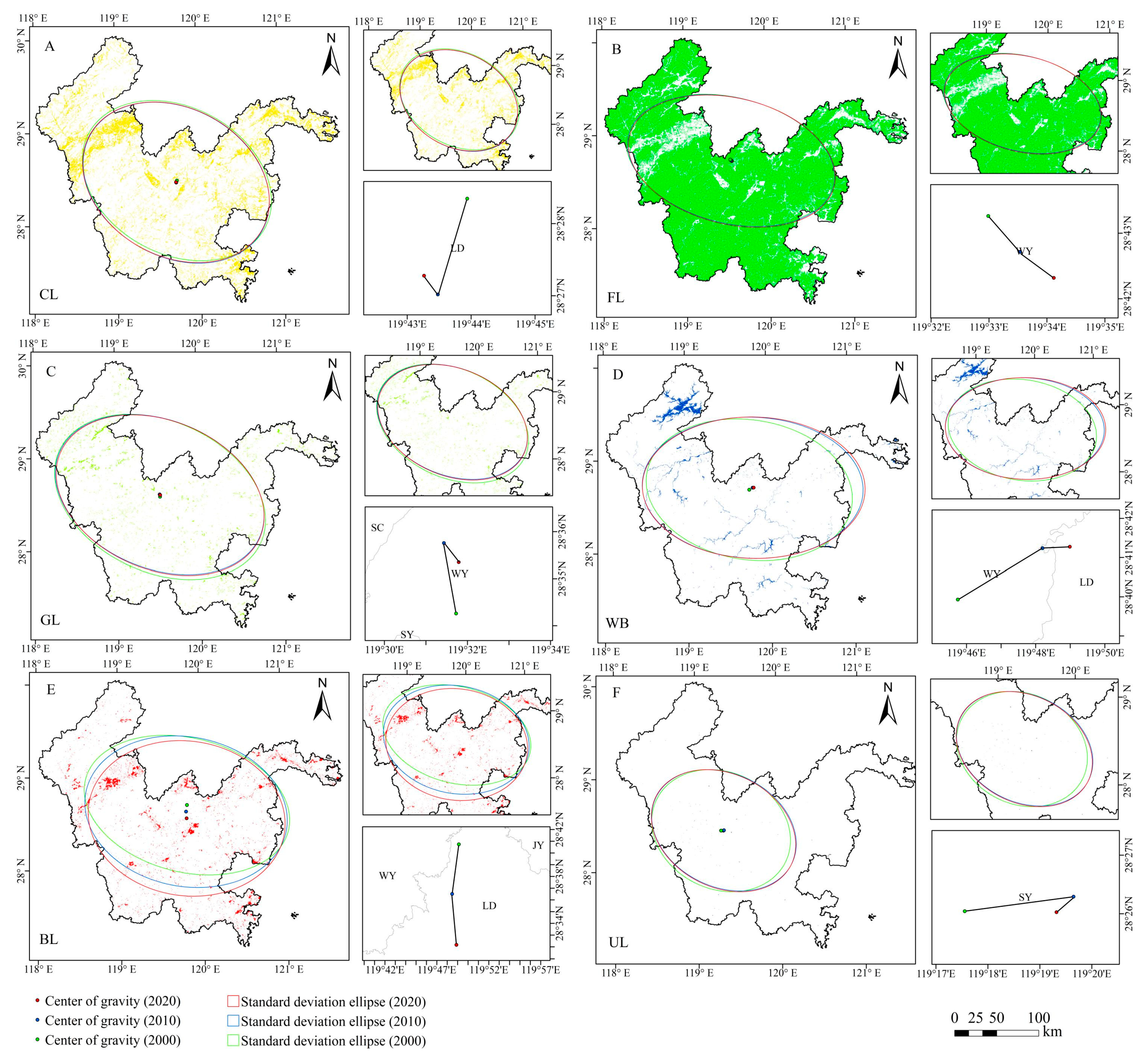
This study further applied the SDE and gravity center models to analyze the spatial characteristics and spatiotemporal evolution of land use categories, with results shown in Figure 4. From 2000 to 2020, the SDE for all land use categories covered most areas, demonstrating relatively stable spatial differentiation patterns. The major axes consistently exhibited a northwest-southeast orientation, indicating greater dispersion of land use distributions along this direction due to the region’s topographic characteristics of higher elevation in the southwest and lower elevation in the northeast. Temporally, SDE underwent significantly greater changes during 2000–2010 than 2010–2020, confirming the earlier decade as the period of more intensive land use transitions. Spatially, BL’s ellipse shifted substantially southward while its minor axis elongated, reflecting more balanced urban-rural development along the north–south dimension driven by accelerated urbanization in southern hilly areas (Figure 4E). Gravity center analysis revealed southward migration for CL, FL, and BL (Figure 4A,B,E), northward migration for GL (Figure 4C), and eastward migration for WB and UL (Figure 4D,F).

3.2. Eco-Environmental Response to Land Use Transformation

3.2.1. Spatio-Temporal Evolution of EEQI

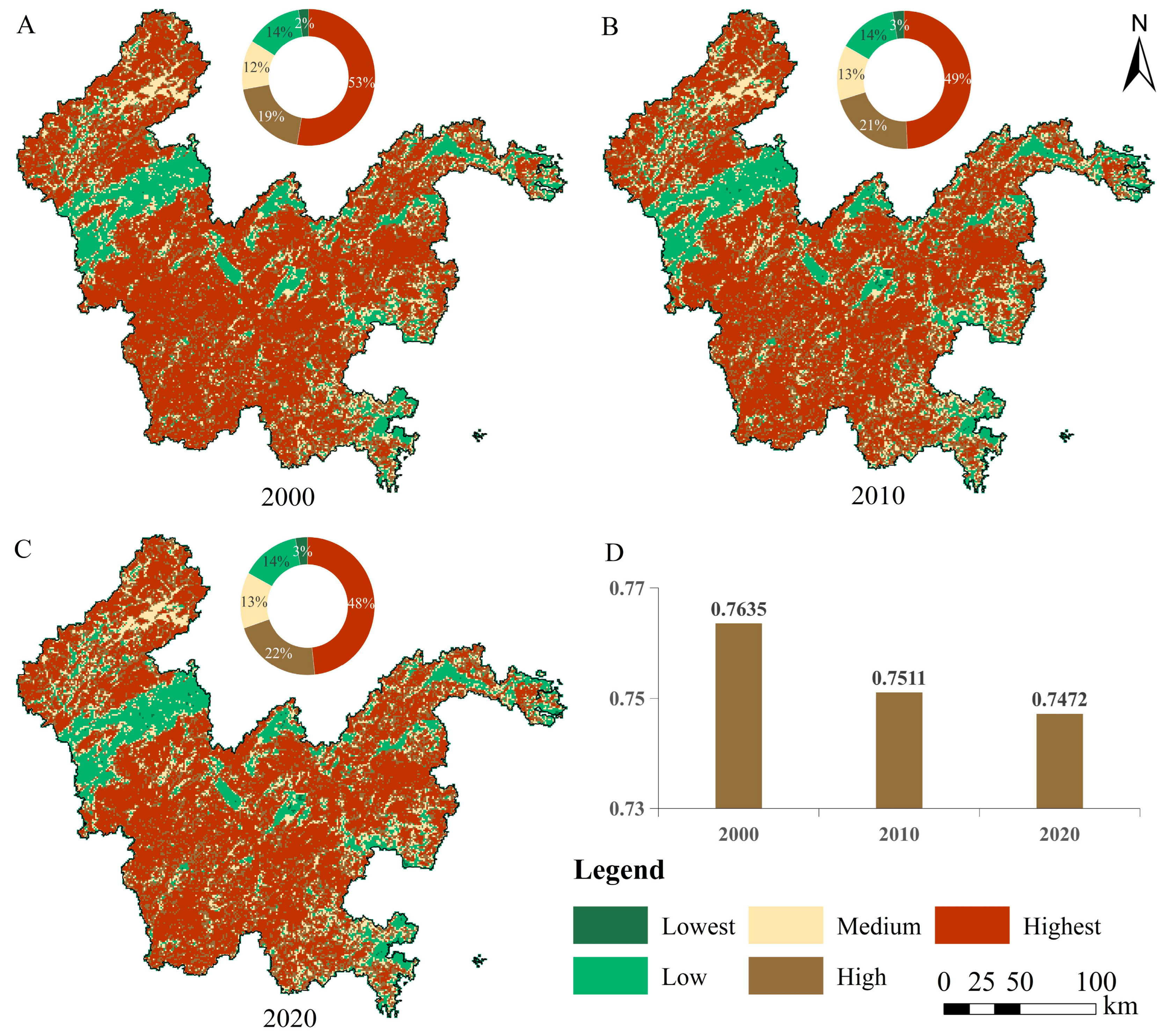
The overall EEQI for the study area was 0.7635, 0.7511, and 0.7472 in 2000, 2010, and 2020, respectively, consistently classified as high level. This indicates generally favorable EEQ conditions across the region. Temporally, EEQI exhibited a slight declining trend over the study period, though the rate of decrease decelerated (Figure 5D). Spatially, grid cells classified as high and highest levels accounted for 19% and 53% of the total area in 2000, while low and lowest levels covered 14% and 2% (Figure 5A). By 2010, the proportion of highest-level grids decreased by 4 percentage points to 49%, and lowest-level grids increased by 1 percentage point to 3% (Figure 5B). In 2020, highest-level grids further declined by 1 percentage point to 48% (Figure 5C). Geographically, EEQI values were notably higher in the southwestern areas and lower in urbanized zones.

3.2.2. Hot Spots of EEQI

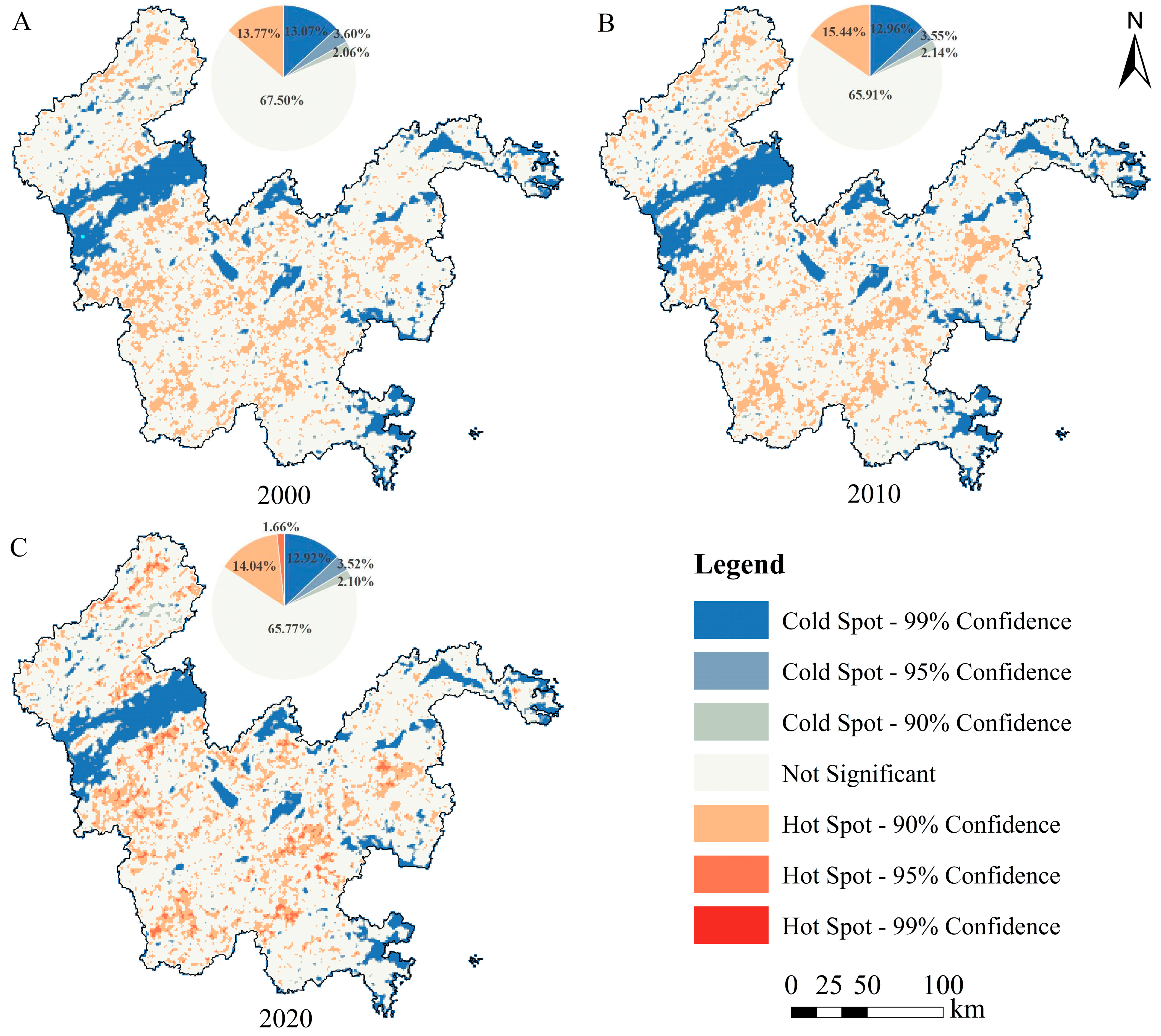
The spatial agglomeration dynamics of EEQI exhibited distinct evolutionary patterns: hot spots demonstrated a qualitative transition from 90% confidence expansion to 95% confidence emergence, while cold spots revealed a paradoxical trend of areal contraction with persistent 99%-confidence resistance (Figure 6). Structurally, hot spots underwent optimization as 90%-confidence hot spot area showed fluctuating growth, indicating expanding ecological improvement. Notably, the inaugural emergence of 95%-confidence hot spots in 2020 marked a transition from quantitative to qualitative improvement in core ecological zones like southwestern Zhejiang (Lishui), evidencing successful conservation in key ecological functional areas. Conversely, cold spots displayed entrenched persistence: 99%-confidence cold spots declined minimally (−0.15%), 95%-confidence cold spots decreased by 0.09%. This pattern signifies a deep-seated lock-in effect of ecological degradation in intensively developed regions.

3.3. Driving Factors of EEQI

3.3.1. Relative Importance Analysis

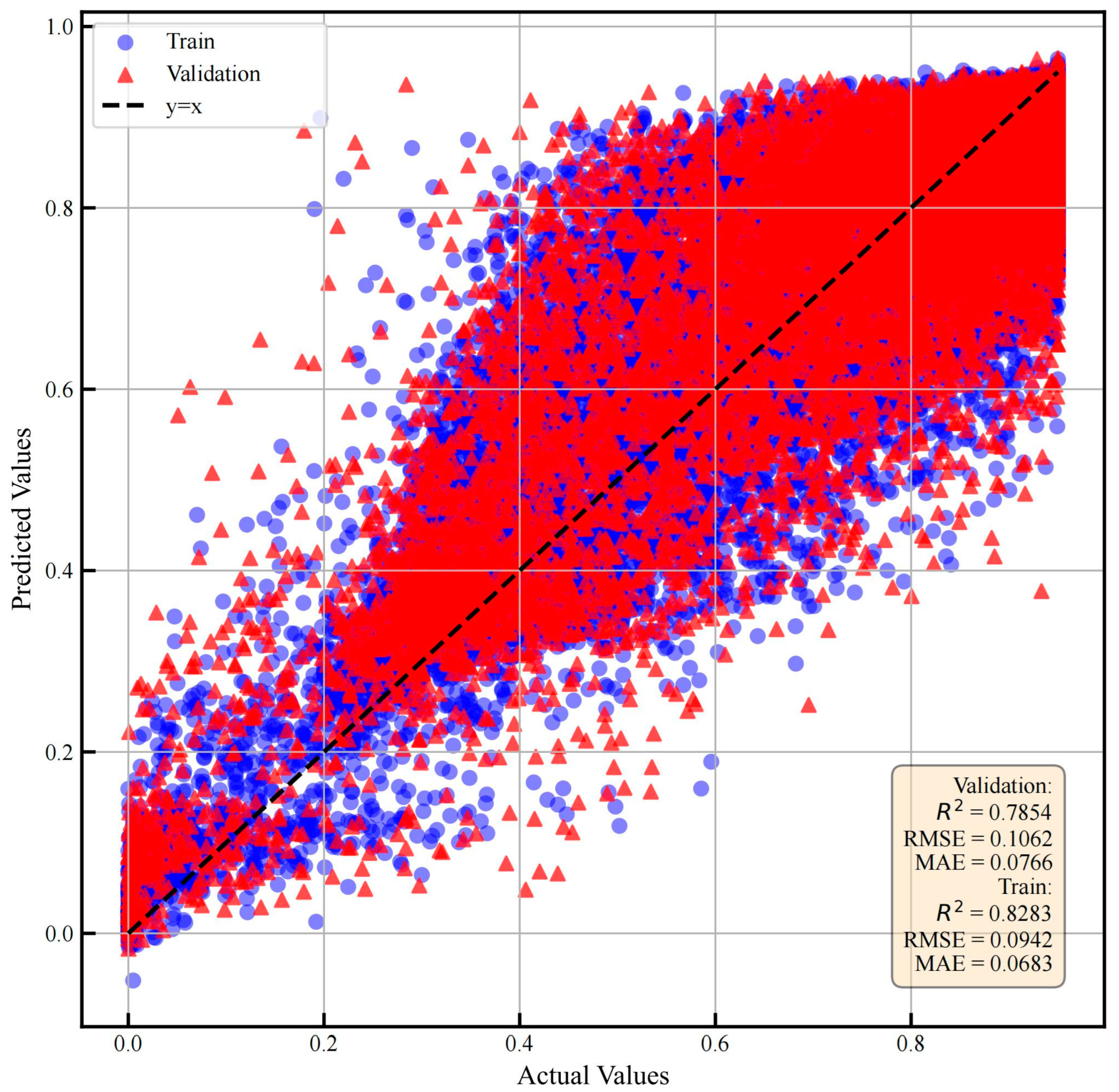
In this study, 70% of the samples were allocated for training the XGBoost model, with the remaining 30% reserved for validation. Automated hyperparameter tuning was performed using GridSearchCV, ultimately identifying the optimal parameter set yielding the highest score (lowest negative mean squared error). The optimized parameters were: learning_rate = 0.05; max_depth = 5; n_estimators = 500. Model accuracy was evaluated by calculating the coefficient of determination (R2) and Root Mean Squared Error (RMSE) for both training and validation sets, where higher R2 and lower RMSE values indicate superior performance. As shown in Figure 7, the XGBoost model achieved R2 = 0.83 (RMSE = 0.09) on the training set and R2 = 0.79 (RMSE = 0.11) on the validation set, demonstrating high predictive accuracy.
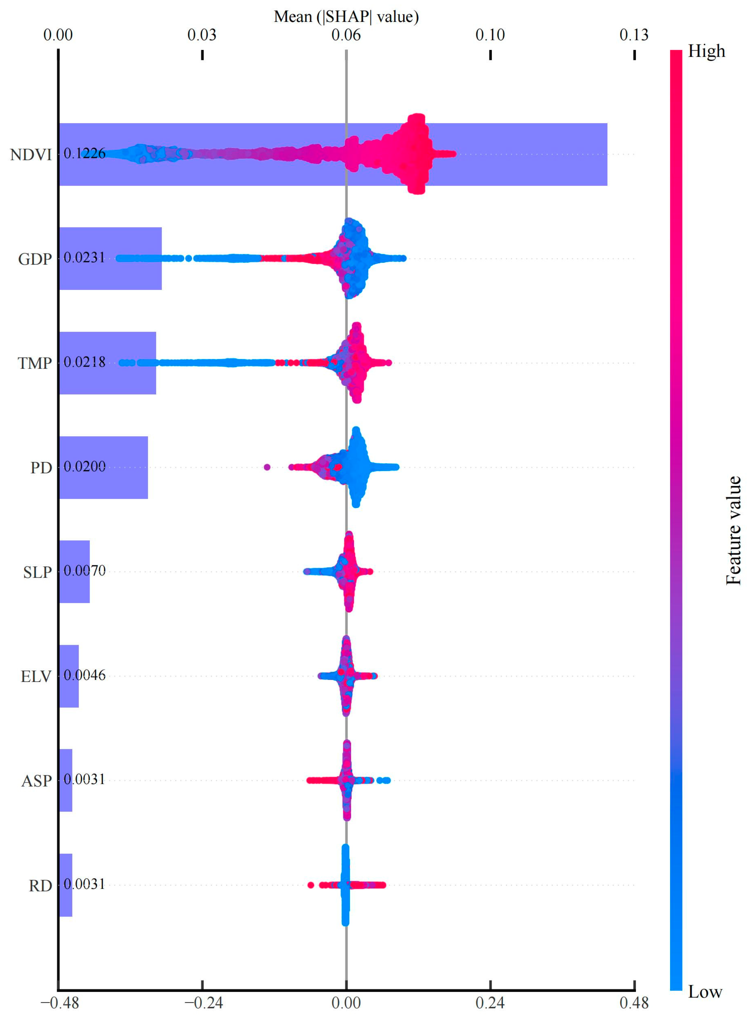
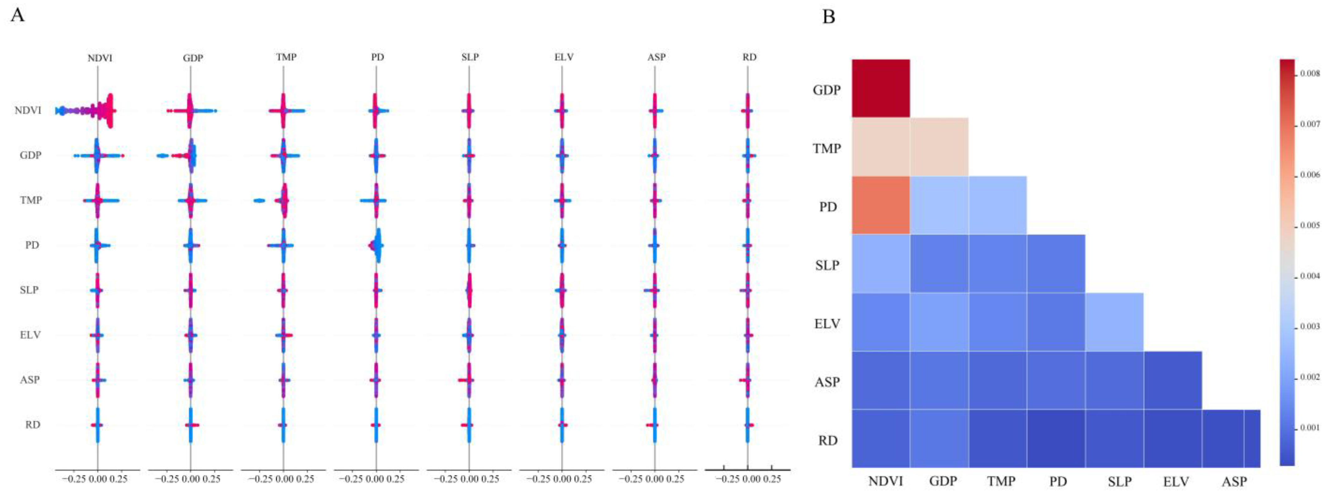
The histogram in Figure 8 presents SHAP-based feature rankings, indicating the relative importance of driving factors on EEQI during the study period, where higher SHAP values denote stronger influence. Ranked by mean absolute SHAP value in descending order, the factors are NDVI, GDP, TMP, PD, SLP, ELV, ASP, RD. NDVI emerged as the most influential factor (SHAP = 0.1226), accounting for over 59% of the total impact, followed by per-unit-area GDP (11.25%) and temperature (10.62%). In the accompanying beeswarm plot, each point represents a sample’s SHAP value, with the x-axis indicating effect direction: left of the vertical line signifies negative impacts and right indicates positive impacts. Red/blue coloring denotes high/low feature values, respectively. Distribution patterns reveal factor effects: NDVI and SLP exhibit positive influences (characterized by right-clustered red points and left-clustered blue points), while PD and ASP show negative influences (right-clustered blue points and left-clustered red points). GDP, TMP, ELV, and RD demonstrate complex nonlinear relationships, evidenced by scattered distributions across both SHAP domains.

3.3.2. Partial Dependence Relationship Between Driving Factors and EEQI

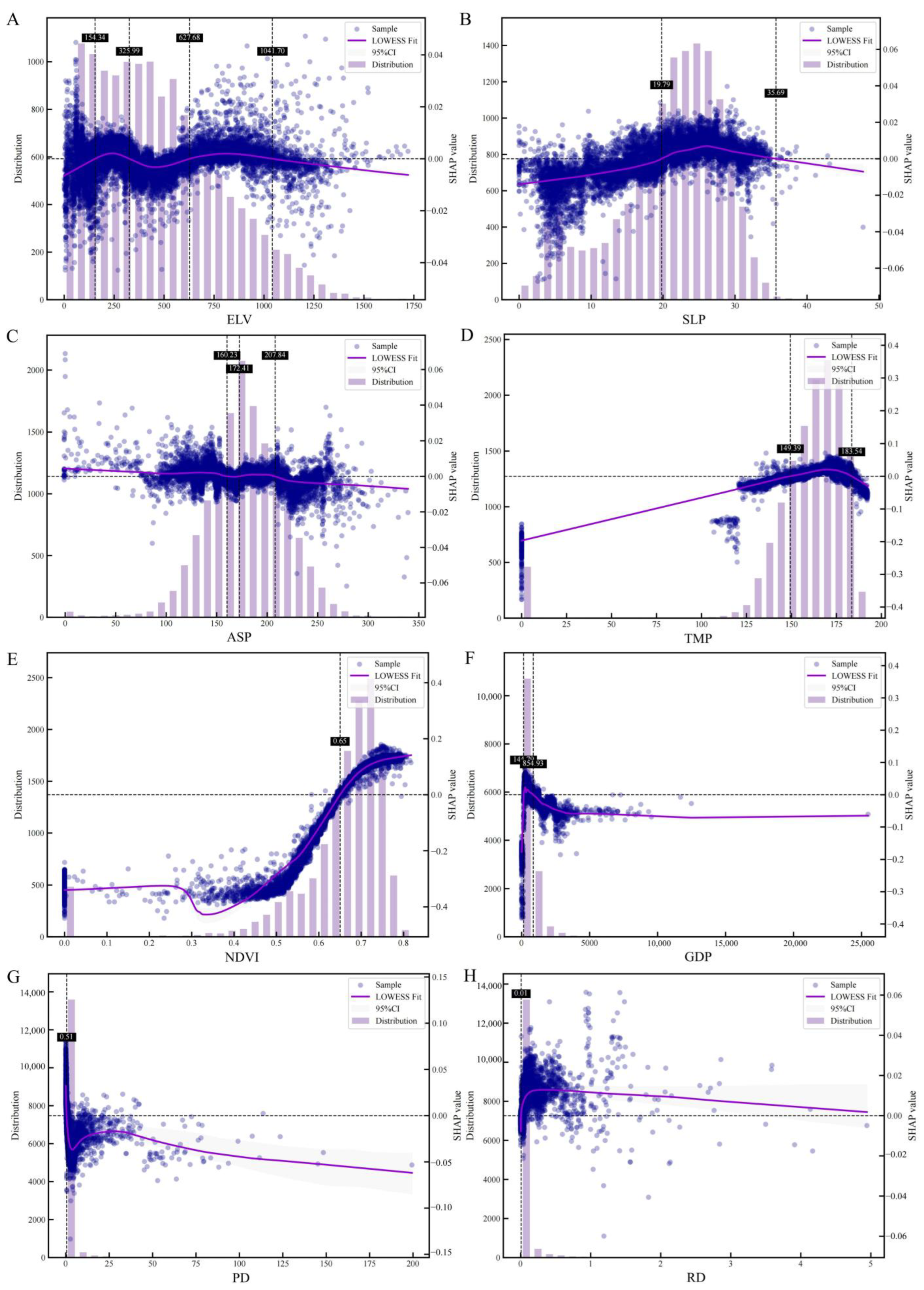
To further elucidate the nonlinear relationships between driving factors and EEQI, Figure 9 presents SHAP dependence plots for eight factors, incorporating scatter points, fitted curves, and density histograms. The x-axis represents feature values of driving factors, while the y-axis denotes corresponding SHAP values. Confidence intervals were estimated using a bootstrap method [48], with fitted curves generated through moving window-based locally estimated scatterplot smoothing (LOWESS) regression [49]. Results reveal: ELV exhibits significant nonlinearity, positive effects occur within 154.34–325.99 m and 627.68–1041.70 m ranges, but negative impacts prevail outside these thresholds. Notably, when ELV exceeds 1041.70 m, SHAP values decrease with increasing elevation (Figure 9A). SLP positively influences EEQI between 19.79 and 35.69°, with negative effects below 19.79° or above 35.69° (Figure 9B). ASP shows a negative correlation with EEQI (Figure 9C). TMP demonstrates positive effects within 149.39–183.54 (units: 0.1 °C), transitioning to negative impacts beyond this range (Figure 9D). NDVI maintains a positive correlation overall, though negative effects emerge when NDVI < 0.65, shifting to positive impacts when NDVI > 0.65 (Figure 9E). Per capita GDP and PD consistently suppress EEQI, while RD enhances it (Figure 9F–H).

3.3.3. Interactions of Driving Factors

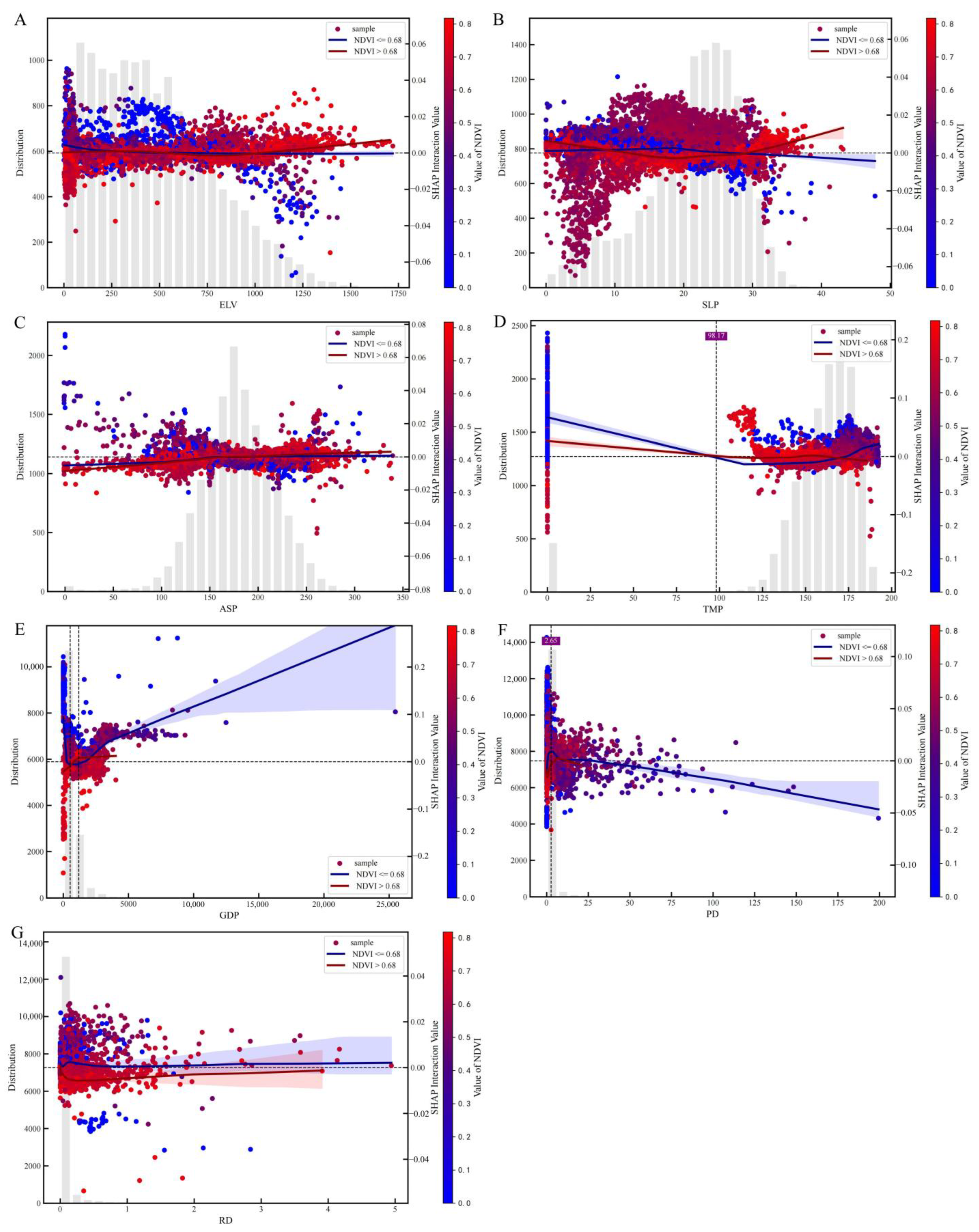
To elucidate the mechanisms through which driving factors influence EEQI, this study evaluated interaction effects among these factors (Figure 10). Results revealed the strongest interaction between per-unit-area GDP and NDVI, followed by PD-NDVI, TMP-NDVI, and TMP-GDP interactions, indicating NDVI’s pronounced interactive role with other variables. Further investigation through interaction plots (Figure 11) visualized NDVI’s interplay with other factors: the x-axis represents alternate factor values, while the right y-axis shows interaction SHAP values. Point coloration reflects NDVI magnitude (red: high NDVI; blue: low NDVI). Samples were stratified into high-value (NDVI > 0.68) and low-value (NDVI ≤ 0.68) groups based on the NDVI median, with separate LOWESS curves fitted for each (red: high group; blue: low group). Interaction effects demonstrated weak positive correlations with ELV and ASP (Figure 11A,C), suggesting synergistic positive impacts on EEQ. The steepest positive slope occurred when per-unit-area GDP exceeded 1187 with low NDVI values (Figure 11E). Conversely, negative correlations emerged with TMP and PD (Figure 11D,F), particularly pronounced in the low-NDVI/PD interaction. RD-NDVI interaction was negligible (Figure 11G). Notably, SLP-NDVI interactions exhibited divergent trends across groups (Figure 11B): high-NDVI samples showed positive correlation with SLP, while low-NDVI samples displayed negative correlation, with an interaction shift threshold near SLP = 30°. This implies cooperative positive EEQ effects for high NDVI on steep slopes (>30°), but antagonistic effects for low NDVI, underscoring the critical importance of vegetation enhancement in steep terrain for ecological resilience.

4. Discussion

4.1. Interpretation of Results and Theoretical Contributions

This study established a “process-effect-driver” analytical framework, revealing the mechanisms of land use transformation and EEQ responses in China’s southern hilly area under the coupled context of “high vegetation cover baseline + rapid urbanization pressure.” This framework advances research on territorial spatial transformation and EEQ in typical hilly ecosystems. By integrating XGBoost and SHAP methods, we overcame limitations of traditional statistical models in identifying nonlinear relationships, quantifying contribution rates and pathways of EEQI drivers in hilly areas, thereby providing theoretical support for adaptive governance of human-land systems. Specific contributions are threefold:
Deciphering ecological effects of land use transformation in hilly areas. Rapid expansion of BL is the core driver of the slight decline in EEQ, primarily through its encroachment on CL and FL. The spatial heterogeneity of EEQI within the region was significant. The result highlights urbanization’s squeeze on ecological spaces and the success of key ecological zone policies, with hotspots marking a shift to substantive restoration.
Unveiling nonlinear mechanisms of EEQI drivers. This study effectively deciphered complex relationships that are difficult to capture with traditional linear models: NDVI is the primary driver of EEQ in hilly areas, exhibiting a significant positive correlation with EEQI and a threshold effect—specifically, when NDVI > 0.65, the positive influence strengthens. This threshold corresponds to the minimum vegetation coverage required for effective soil conservation, microclimate regulation, and biodiversity maintenance. Socioeconomic factors demonstrated a dual-edged effect: per capita GDP and PD generally suppressed EEQ, yet the impact of GDP showed inflection points across intervals, suggesting potential room for coordination between economic development and ecological protection. The study also revealed pronounced nonlinear characteristics in natural topographic factors, providing precise target areas for ecological restoration on steep slopes.
Quantifying nonlinear interaction effects: The NDVI-GDP interaction showed the strongest contribution, indicating vegetation cover can buffer economic development’s ecological costs. The SLP-NDVI synergy proved critical: when SLP>30°, high NDVI substantially amplified EEQ gains. This discovery deepens understanding of the “topography-vegetation” coupling mechanism and provides a theoretical anchor for soil-water conservation and biodiversity protection in hilly area.

4.2. Comparative Analysis

The mechanisms of EEQ response to territorial spatial transformation and its drivers in China’s southern hilly area, as revealed in this study, engage with existing literature through multidimensional dialog while highlighting regional specificity and theoretical innovation. Key comparative insights are:
This study found that the rapid expansion of BL led to a slight decline in EEQ, with cold spots concentrated predominantly in urban belts. This finding is consistent with research in multiple urbanized regions, which identifies construction land expansion as a core driver of EEQ degradation [29]. Meanwhile, ecological policies were observed to exert a buffering effect: despite the encroachment of BL, hotspot areas increased, confirming the effectiveness of policies such as the Grain for Green Program and the development of ecological functional zones. This aligns with the findings of related studies [50,51], underscoring the significant benefits of ecological restoration initiatives on EEQ. Regarding regional heterogeneity, unlike studies conducted in arid areas [52], this region—characterized by high vegetation coverage—experiences simultaneous urbanization pressure and ecological restoration, presenting a more complex “squeeze-restoration” equilibrium model.
Traditional linear models, such as geographical detector and GWR, often overlook threshold effects and complex interactions among driving factors [53,54]. This study overcame these limitations through the XGBoost-SHAP model, which not only confirmed the dominant role of NDVI in influencing EEQI but also identified a significant threshold effect. This finding is consistent with multiple studies [55]. Previous research has shown that high vegetation coverage enhances ecosystem stability by improving soil-water conservation and carbon sequestration capacity, thereby exerting a positive influence on EEQ [56,57]. Regarding socioeconomic factors, existing studies have discussed the effects of GDP and PD on EEQI, revealing generally negative impacts [58,59,60], which aligns with the results of this study. In contrast, RD was found to have a positive effect on EEQI, which can be attributed to improved infrastructure and management practices in hilly areas over the past two decades. Within the context of Zhejiang’s “Beautiful Countryside” initiative, higher road density is often associated with ecological management, nature-based tourism development, and village renovation projects that include greening and environmental protection measures [61]. This suggests that under specific policy conditions, infrastructure construction can be synergistically aligned with environmental improvement. Moreover, the complex nonlinear characteristics of topographic factors identified in this study have also been observed in recent related research [62].
This study revealed that when SLP > 30°, the positive contribution of high NDVI to EEQI is significantly amplified. This SLP threshold represents a critical gradient where human disturbance diminishes and natural vegetation becomes dominant. It also indicates that vegetation restoration on steep slopes can effectively reduce erosion and enhance ecological resilience, highlighting the importance of slope-vegetation coupling. Related studies have similarly identified a range of 25–69.7° within which SLP exerts improving effects on EEQ, consistent with the findings of this research [63].

4.3. Policy Evolution and Phased Characteristics of EEQ Response

Due to data availability constraints, this study primarily considered natural and socioeconomic drivers of EEQI without quantifying policy impacts. Nevertheless, Zhejiang’s hilly areas underwent profound territorial spatial transformation during 2000–2020, where phased policy orientations significantly shaped land use patterns and EEQI dynamics. Based on documented policy practices, we interpret policy influences on EEQI as follows:
2000–2010: Preliminary balance between gentle slope development and ecological protection. The policy focus centered on resolving conflicts between CL preservation and urbanization through gentle slope development to expand construction space. Specifically, pilot initiatives launched in 2005 promoted industrial park development on gentle slopes (6–15°). While reducing encroachment on plain CL, this triggered substantial FL-to-BL conversion, becoming a primary contributor to EEQI decline. Concurrently, preliminary ecological conservation measures emerged: the 2008 Zhejiang Land Use Master Plan designated ecological source areas in hilly area as “provincial ecological barriers and riverhead protection zones”, enabling counties with high forest coverage (e.g., Longquan, Suichang) in southwestern Zhejiang to maintain stable EEQ.
2010–2020: Policy upgrading under ecological priority. Policies shifted toward ecological value realization and refined governance, arresting EEQI degradation. The “Slope Village-Town” initiative (2015 pilot) adopted a “point-based layout, vertical development” model under the principle of “zero cropland occupation, minimal agricultural land conversion”, pursuing triple objectives of conserving cultivated land, ecology, and development. Simultaneously, deepened forest tenure reforms introduced innovations like forest-right mortgages, promoting forest area expansion and demonstrating the beneficial effects of vegetation cover on steep slope ecological restoration.
Over the past two decades, Zhejiang has implemented policies such as the “Thousand-Village Demonstration and Ten-Thousand-Village Improvement” project to synergistically advance land consolidation, ecological restoration, and rural revitalization. This approach is now being promoted in other regions across China. Zhejiang’s experience demonstrates that integrating ecological priorities into land use planning and policy implementation can effectively mitigate environmental degradation while supporting sustainable development. Practices such as slope-based development controls, forest tenure reforms, and ecological protection redlines offer valuable insights for other hilly areas in southern China and beyond—particularly those undergoing rapid urbanization and ecological transition. Moreover, this model provides a reference for similar regions globally, demonstrating a viable pathway to balance ecological conservation with economic development.

4.4. Limitations and Future Research Directions

This study systematically revealed the spatiotemporal response characteristics of EEQI to territorial spatial transformation and its nonlinear driving mechanisms in China’s southern hilly area, yet several limitations persist: Insufficient integration and quantification of policy drivers obscure direct contributions of policy interventions and their coupling effects with land use transformation. The decadal interval may overlook short-term dynamics and transitional phases, while future scenario projections (e.g., land use evolution under climate change) remain unexplored. Analysis at the 1 km grid scale potentially overlooks finer ecological processes and mechanisms at the parcel level. The composite index approach cannot disentangle pathways and tradeoffs/synergies of land use transformation impacts on specific ecosystem services.
Future research should prioritize: constructing policy indicator systems using text mining and causal analysis to quantify policy intensity and orientation; capturing short-term EEQI fluctuations and simulating future trajectories under diverse scenarios (ecological/economic priority, balanced development) to inform proactive spatial planning; conducting high-resolution case studies in typical watersheds to validate macro-scale mechanisms; integrating EEQI with ecosystem service models (e.g., InVEST) to quantify impacts on service flows and spatial tradeoffs/synergies, enabling precision conservation.

5. Conclusions

This study established an integrated analytical framework to decipher the spatio-temporal evolution and driving factors of EEQ in China’s southern hilly area. The core findings are: (1) Rapid BL expansion, at the expense of CL and FL, was the primary driver of a slight but persistent decline in EEQI, with clear spatial disparities between urbanizing zones (degradation) and ecological conservation areas (improvement). (2) Driving factors exhibited complex nonlinear relationships, with NDVI identified as the dominant positive factor, exhibiting a critical threshold effect (>0.65). (3) Significant factor interactions were identified, most notably the coupling mechanism between slope and vegetation: on steeper slopes (>30°), high vegetation cover substantially amplified ecological benefits.
The application of the XGBoost-SHAP framework proved highly effective in uncovering these complex, nonlinear mechanisms, offering a superior approach compared to traditional linear models for human-land system research. These insights highlight the critical importance of protecting and restoring vegetation on steep slopes and suggest that economic development can be better coordinated with ecological conservation. The findings provide a scientific basis for precise land-use planning and ecological restoration strategies not only in the study area but also in other hilly regions facing similar development pressures.

Author Contributions

Conceptualization, Z.X.; methodology, Z.X.; software, Z.X.; validation, Z.X.; formal analysis, Z.X.; investigation, Z.X.; resources, Z.X.; data curation, Z.X.; writing—original draft preparation, Z.X.; writing—review and editing, Z.X.; visualization, Z.X. and H.Z.; supervision, Z.X. and F.K.; project administration, Z.X. and J.Y.; funding acquisition, Z.X. and F.K. All authors have read and agreed to the published version of the manuscript.

Funding

This research was funded by Zhejiang Academy of Agricultural Sciences, grant number 2025R18Y11E11.

Conflicts of Interest

The authors declare no conflicts of interest. The funders had no role in the design of the study; in the collection, analyses, or interpretation of data; in the writing of the manuscript; or in the decision to publish the results.

Abbreviations

The following abbreviations are used in this manuscript:
EEQEco-environment quality
EEQIEco-environment quality index
CLCropland
FLForestland
GLGrassland
WBWater Bodies
BLBuilt-up Land
ULUnused Land
SDEStandard Deviational Ellipse
XGBoostExtreme Gradient Boosting
SHAPSHapley Additive exPlanations

References

  1. Zhou, G.; Long, H. Explanation of land-use system evolution: Modes, trends, and mechanisms. Land Use Policy 2025, 150, 107470. [Google Scholar] [CrossRef]
  2. Zhu, T.; Qin, X. Urbanization path: The fundamental problem of changes in land use patterns. Sci. Geogr. Sin. 2012, 32, 1348–1352. [Google Scholar]
  3. Liu, Y.S.; Zang, Y.Z.; Yang, Y.Y. China’s rural revitalization and development: Theory, technology and management. J. Geogr. Sci. 2020, 30, 1923–1942. [Google Scholar] [CrossRef]
  4. Xu, X.B.; Yang, G.S.; Tan, Y. Identifying ecological red lines in China’s yangtze river economic belt: A regional approach. Ecol. Indic. 2019, 96, 635–646. [Google Scholar] [CrossRef]
  5. Tao, J.; Lu, Y.; Ge, D.; Dong, P.; Gong, X.; Ma, X. The spatial pattern of agricultural ecosystem services from the production-living-ecology perspective: A case study of the huaihai economic zone, China. Land Use Policy 2022, 122, 106355. [Google Scholar] [CrossRef]
  6. Dadashpoor, H.; Azizi, P.; Moghadasi, M. Land use change, urbanization, and change in landscape pattern in a metropolitan area. Sci. Total Environ. 2019, 655, 707–719. [Google Scholar] [CrossRef]
  7. Cao, Y.; Zhang, M.Y.; Zhang, Z.Y.; Liu, L.; Gao, Y.; Zhang, X.Y.; Chen, H.J.; Kang, Z.W.; Liu, X.Y.; Zhang, Y. The impact of land-use change on the ecological environment quality from the perspective of production-living-ecological space: A case study of the northern slope of tianshan mountains. Ecol. Inform. 2024, 83, 102795. [Google Scholar] [CrossRef]
  8. Sun, T.; Yang, Y.; Wang, Z.; Yong, Z.; Xiong, J.; Ma, G.; Li, J.; Liu, A. Spatiotemporal variation of ecological environment quality and extreme climate drivers on the qinghai-tibetan plateau. J. Mt. Sci. 2023, 20, 2282–2297. [Google Scholar] [CrossRef]
  9. Zhang, Y.; Liu, Y.; Gu, J. Land use/land cover change and its environmental effects in wuhan city. Geogr. Sci. 2011, 31, 1280–1285. [Google Scholar]
  10. Gari, S.R.; Newton, A.; Icely, J.D. A review of the application and evolution of the DPSIR framework with an emphasis on coastal social-ecological systems. Ocean Coast. Manag. 2015, 103, 63–77. [Google Scholar] [CrossRef]
  11. Hu, X.S.; Xu, H.Q. A new remote sensing index for assessing the spatial heterogeneity in urban ecological quality: A case from fuzhou city, China. Ecol. Indic. 2018, 89, 11–21. [Google Scholar] [CrossRef]
  12. Yang, L.; Liu, Y.; Liu, Y.; Liu, R. Spatial-temporal dynamics and drivers of ecosystem service interactions along the yellow river area in shaanxi province. J. Clean. Prod. 2025, 496, 145095. [Google Scholar] [CrossRef]
  13. Yu, B.B. Ecological effects of new-type urbanization in China. Renew. Sust. Energ. Rev. 2021, 135, 110239. [Google Scholar] [CrossRef]
  14. Wang, J.T.; Peng, J.; Zhao, M.Y.; Liu, Y.X.; Chen, Y.Q. Significant trade-off for the impact of grain-for-green programme on ecosystem services in north-western yunnan, China. Sci. Total Environ. 2017, 574, 57–64. [Google Scholar] [CrossRef]
  15. Yang, L.; Shi, L.; Wei, J.; Wang, Y. Spatiotemporal evolution of ecological environment quality in arid areas based on the remote sensing ecological distance index: A case study of yuyang district in yulin city, China. Open Geosci. 2021, 13, 1701–1710. [Google Scholar] [CrossRef]
  16. Zhang, Y.; Peng, C.H.; Li, W.Z.; Tian, L.X.; Zhu, Q.Q.; Chen, H.; Fang, X.Q.; Zhang, G.L.; Liu, G.M.; Mu, X.M.; et al. Multiple afforestation programs accelerate the greenness in the ‘three north’ region of China from 1982 to 2013. Ecol. Indic. 2016, 61, 404–412. [Google Scholar] [CrossRef]
  17. Li, K.; Wu, W.; Tian, S.; Li, L.; Li, Z.; Cao, Y. Geographical feature and method factors significantly influence the reliability of ecological source information transmission at multi-scale. Ecol. Indic. 2025, 170, 113029. [Google Scholar] [CrossRef]
  18. Chen, Y.; Lu, Y.; Meng, R.; Li, S.; Zheng, L.; Song, M. Multi-scale matching and simulating flows of ecosystem service supply and demand in the wuhan metropolitan area, China. J. Clean. Prod. 2024, 476, 143648. [Google Scholar] [CrossRef]
  19. Su, X.Y.; Fan, Y.M.; Wen, C.H. Systematic coupling and multistage interactive response of the urban land use efficiency and ecological environment quality. J. Environ. Manag. 2024, 365, 121584. [Google Scholar] [CrossRef] [PubMed]
  20. Li, C.; Jin, Z.; Jiang, C.C.; Shen, Y.J.; Wang, R.; Peng, J.B. Coupled mutual feedback and interaction mechanisms among the geological environment, ecological environment and human activities in the qinling mountains. Sci. China Earth Sci. 2025, 68, 2663–2682. [Google Scholar] [CrossRef]
  21. Song, Y.; Wang, J.; Ge, Y.; Xu, C. An optimal parameters-based geographical detector model enhances geographic characteristics of explanatory variables for spatial heterogeneity analysis: Cases with different types of spatial data. GISci. Remote Sens. 2020, 57, 593–610. [Google Scholar] [CrossRef]
  22. Chen, W.Y.; Zhao, R.F.; Lu, H.T. Response of ecological environment quality to land use transition based on dryland oasis ecological index (DOEI) in dryland: A case study of oasis concentration area in middle heihe river, China. Ecol. Indic. 2024, 165, 112214. [Google Scholar] [CrossRef]
  23. Xu, Z.; Ke, F.; Yu, J. Spatio-temporal evolution and influencing factors of rural production-living-ecological function: A case study of mountainous counties in zhejiang province, China. Front. Environ. Sci. 2025, 13, 1495778. [Google Scholar] [CrossRef]
  24. Ning, J.; Liu, J.Y.; Kuang, W.H.; Xu, X.L.; Zhang, S.W.; Yan, C.Z.; Li, R.D.; Wu, S.X.; Hu, Y.F.; Du, G.M.; et al. Spatiotemporal patterns and characteristics of land-use change in China during 2010–2015. J. Geogr. Sci. 2018, 28, 547–562. [Google Scholar] [CrossRef]
  25. Xu, X. 1 km-Grid Dataset of Spatial Distribution of China’s GDP. Available online: https://www.resdc.cn/DOI/DOI.aspx?DOIID=33 (accessed on 21 April 2025).
  26. Peng, S. 1-km Monthly Mean Temperature Dataset for China (1901–2023); National Tibetan Plateau Data Center: Beijing, China, 2024. [Google Scholar]
  27. Didan, K. MOD13a3 MODIS/Terra Vegetation Indices Monthly l3 Global 1km SIN Grid v006; NASA EOSDIS Land Processes Distributed Active Archive Center: Sioux Falls, SD, USA, 2015. [Google Scholar]
  28. Yang, Q.; Duan, X.; Wang, L.; Jin, Z. Land use transformation based on ecological-production-living spaces and associated eco-environment effects: A case study in the yangtze river delta. Sci. Geogr. Sin. 2018, 38, 97–106. [Google Scholar]
  29. Hu, C.; Song, M.; Zhang, A. Dynamics of the eco-environmental quality in response to land use changes in rapidly urbanizing areas: A case study of wuhan, China from 2000 to 2018. J. Geogr. Sci. 2023, 33, 245–265. [Google Scholar] [CrossRef]
  30. Hilgard, J.E. The advance of population in the united states. Scribner’s Mon. 1872, 4, 214–218. [Google Scholar]
  31. Zhang, G.; Zhang, N.; Liao, W. How do population and land urbanization affect CO2 emissions under gravity center change? A spatial econometric analysis. J. Clean. Prod. 2018, 202, 510–523. [Google Scholar] [CrossRef]
  32. Sherman, J.E.; Spencer, J.; Preisser, J.S.; Gesler, W.M.; Arcury, T.A. A suite of methods for representing activity space in a healthcare accessibility study. Int. J. Health Geogr. 2005, 4, 24. [Google Scholar] [CrossRef]
  33. Wachowicz, M.; Liu, T. Finding spatial outliers in collective mobility patterns coupled with social ties. Geogr. Inf. Syst. 2016, 30, 1806–1831. [Google Scholar] [CrossRef]
  34. Du, Q.; Zhou, J.; Pan, T.; Sun, Q.; Wu, M. Relationship of carbon emissions and economic growth in China’s construction industry. J. Clean. Prod. 2019, 220, 99–109. [Google Scholar] [CrossRef]
  35. Li, X.; Fang, C.; Huang, J.; Mao, H. The urban land use transformations and associated effects on eco-environment in nothwest China arid region: A case study in hexi region, gansu province. Quat. Sci. 2003, 23, 280–290. [Google Scholar]
  36. Lv, L.; Zhou, S.; Zhou, B.; Dai, L.; Chang, T.; Bao, G.; Zhou, H.; Li, Z. Land use transformation and its eco-environmental response in process of the regional development: A case study of jiangsu province. Sci. Geogr. Sin. 2013, 33, 1442–1449. [Google Scholar]
  37. Getis, A.; Ord, J.K. Local spatial statistics: An overview. In Spatial Analysis: Modeling in a GIS Environment; Longley, P., Batty, M., Eds.; Geoinformation International: Cambridge, UK, 1996; pp. 261–277. [Google Scholar]
  38. Zhang, L.; Fang, C.; Zhao, R.; Zhu, C.; Guan, J. Spatial–temporal evolution and driving force analysis of eco-quality in urban agglomerations in China. Sci. Total Environ. 2023, 866, 161465. [Google Scholar] [CrossRef]
  39. Li, J.S.; Sun, W.; Li, M.Y.; Meng, L.L. Coupling coordination degree of production, living and ecological spaces and its influencing factors in the yellow river basin. J. Clean. Prod. 2021, 298, 126803. [Google Scholar] [CrossRef]
  40. Huang, J.T.; Zhang, Y.C.; Zhang, J.Q.; Qi, J.W.; Liu, P. Study on the ecological environment quality and its driving factors of the spatial transformation of production-living-ecological space in baishan city. Sci. Rep. 2024, 14, 18709. [Google Scholar] [CrossRef]
  41. Hayes, A.F.; Cai, L. Using heteroskedasticity-consistent standard error estimators in OLS regression: An introduction and software implementation. Behav. Res. Methods 2007, 39, 709–722. [Google Scholar] [CrossRef]
  42. Guo, J.; Liao, W.; Qimuge, H.; Xu, Y.; Wang, J. Seasonal analysis of spatial and temporal variations in NDVI and its driving factors in inner mongolia during the vegetation growing season (1999–2019). Front. For. Glob. Change 2025, 8, 1555385. [Google Scholar] [CrossRef]
  43. Chen, T.; Guestrin, C. XGBoost: A scalable tree boosting system. In Proceedings of the 22nd ACM Sigkdd International Conference on Knowledge Discovery and Data Mining, San Francisco, CA, USA, 13–17 August 2016; Association for Computing Machinery: New York, NY, USA, 2016; pp. 785–794. [Google Scholar]
  44. Ma, M.; Zhao, G.; He, B.; Li, Q.; Dong, H.; Wang, S.; Wang, Z. XGBoost-based method for flash flood risk assessment. J. Hydrol. 2021, 598, 126382. [Google Scholar] [CrossRef]
  45. Wu, N.; Zhou, Y.; Yin, S.; Gong, H.; Zhang, C. Revealing the nonlinear impact of environmental regulation on ecological resilience using the XGBoost-SHAP model: Evidence from the yangtze river delta region, China. J. Clean. Prod. 2025, 514, 145700. [Google Scholar] [CrossRef]
  46. Lundberg, S.M.; Lee, S. A unified approach to interpreting model predictions. In Proceedings of the Advances in Neural Information Processing Systems 30 (NIPS 2017), Long Beach, CA, USA, 4–9 December 2017; NIPS Foundation: Red Hook, NY, USA, 2017; pp. 4768–4777. [Google Scholar]
  47. Qi, J.; Xiong, W.; Li, J.; Zheng, J.; Ye, Q.; Hu, M. Investigating non-linear and synergistic effects of urban functional zone morphology on land surface temperature. Sust. Cities Soc. 2025, 130, 106546. [Google Scholar] [CrossRef]
  48. Li, Z. Extracting spatial effects from machine learning model using local interpretation method: An example of SHAP and XGBoost. Comput. Environ. Urban Syst. 2022, 96, 101845. [Google Scholar] [CrossRef]
  49. Zhang, X.; Lin, E.S.; Tan, P.Y.; Qi, J.; Ho, R.; Sia, A.; Waykool, R.; Song, X.P.; Olszewska-Guizzo, A.; Meng, L.; et al. Beyond just green: Explaining and predicting restorative potential of urban landscapes using panorama-based metrics. Landsc. Urban Plan. 2024, 247, 105044. [Google Scholar] [CrossRef]
  50. Yu, Z.Y.; Deng, X.Z.; Cheshmehzangi, A. The grain for green program enhanced synergies between ecosystem regulating services in loess plateau, China. Remote Sens. 2022, 14, 5940. [Google Scholar] [CrossRef]
  51. Jiang, L.; Liu, Y.; Wu, S.; Yang, C. Analyzing ecological environment change and associated driving factors in China based on NDVI time series data. Ecol. Indic. 2021, 129, 107933. [Google Scholar] [CrossRef]
  52. Liu, H.J.; Chen, B.Z.; Xia, Q.Q.; Zabi, G.; Li, G.F. Study on the complex relationship of tourism-economy-ecological environment in arid zones: The case of xinjiang, China. Front. Environ. Sci. 2024, 12, 1435660. [Google Scholar] [CrossRef]
  53. Liu, J.C.; Xie, T.; Lyu, D.; Cui, L.; Liu, Q.M. Analyzing the spatiotemporal dynamics and driving forces of ecological environment quality in the qinling mountains, China. Sustainability 2024, 16, 3251. [Google Scholar] [CrossRef]
  54. Yang, H.H.; Yu, J.; Xu, W.Z.; Wu, Y.; Lei, X.Y.; Ye, J.N.; Geng, J.W.; Ding, Z. Long-time series ecological environment quality monitoring and cause analysis in the dianchi lake basin, China. Ecol. Indic. 2023, 148, 110084. [Google Scholar] [CrossRef]
  55. Dang, L.; Zhao, F.; Teng, Y.; Teng, J.; Zhan, J.; Zhang, F.; Liu, W.; Wang, L. Scale dependency of trade-offs/synergies analysis of ecosystem services based on bayesian belief networks: A case of the yellow river basin. J. Environ. Manag. 2025, 375, 124410. [Google Scholar] [CrossRef]
  56. Lu, Y.; Yu, Y.; Sun, L.; Li, C.; He, J.; Guo, Z.; Duan, L.; Zhang, J.; Yu, R. NDVI based vegetation dynamics and responses to climate change and human activities at xinjiang from 2001 to 2020. Sci. Rep. 2025, 15, 25848. [Google Scholar] [CrossRef]
  57. Xu, J.; Hang, N.T.; Ran, M.; Kong, J. Spatiotemporal dynamics and drivers of vegetation carbon sinks in zhejiang province: A case study in rapidly urbanizing subtropical ecosystems. Plants 2025, 14, 1151. [Google Scholar] [CrossRef] [PubMed]
  58. Chen, X.F.; Liu, C.; Yu, X.H. Urbanization, economic development, and ecological environment: Evidence from provincial panel data in China. Sustainability 2022, 14, 1124. [Google Scholar] [CrossRef]
  59. Fan, Z.M.; Bai, X.Y.; Zhao, N. Explicating the responses of NDVI and GDP to the poverty alleviation policy in poverty areas of China in the 21st century. PLoS ONE 2022, 17, e0271983. [Google Scholar] [CrossRef] [PubMed]
  60. Ren, Y.T.; Zhang, F.; Zhao, C.L.; Cheng, Z.Q. Attribution of climate change and human activities to vegetation NDVI in jilin province, China during 1998–2020. Ecol. Indic. 2023, 153, 110415. [Google Scholar] [CrossRef]
  61. Zhao, Y.; Li, R. Coupling and coordination analysis of digital rural construction from the perspective of rural revitalization: A case study from zhejiang province of China. Sustainability 2022, 14, 3638. [Google Scholar] [CrossRef]
  62. Li, T.; Wang, X.; Jia, H. Evaluate water yield and soil conservation and their environmental gradient effects in fujian province in south China based on InVEST and geodetector models. Water 2025, 17, 230. [Google Scholar] [CrossRef]
  63. Wang, X.; Liu, G.; Xiang, A.; Xiao, S.; Lin, D.; Lin, Y.; Lu, Y. Terrain gradient response of landscape ecological environment to land use and land cover change in the hilly watershed in south China. Ecol. Indic. 2023, 146, 109797. [Google Scholar] [CrossRef]
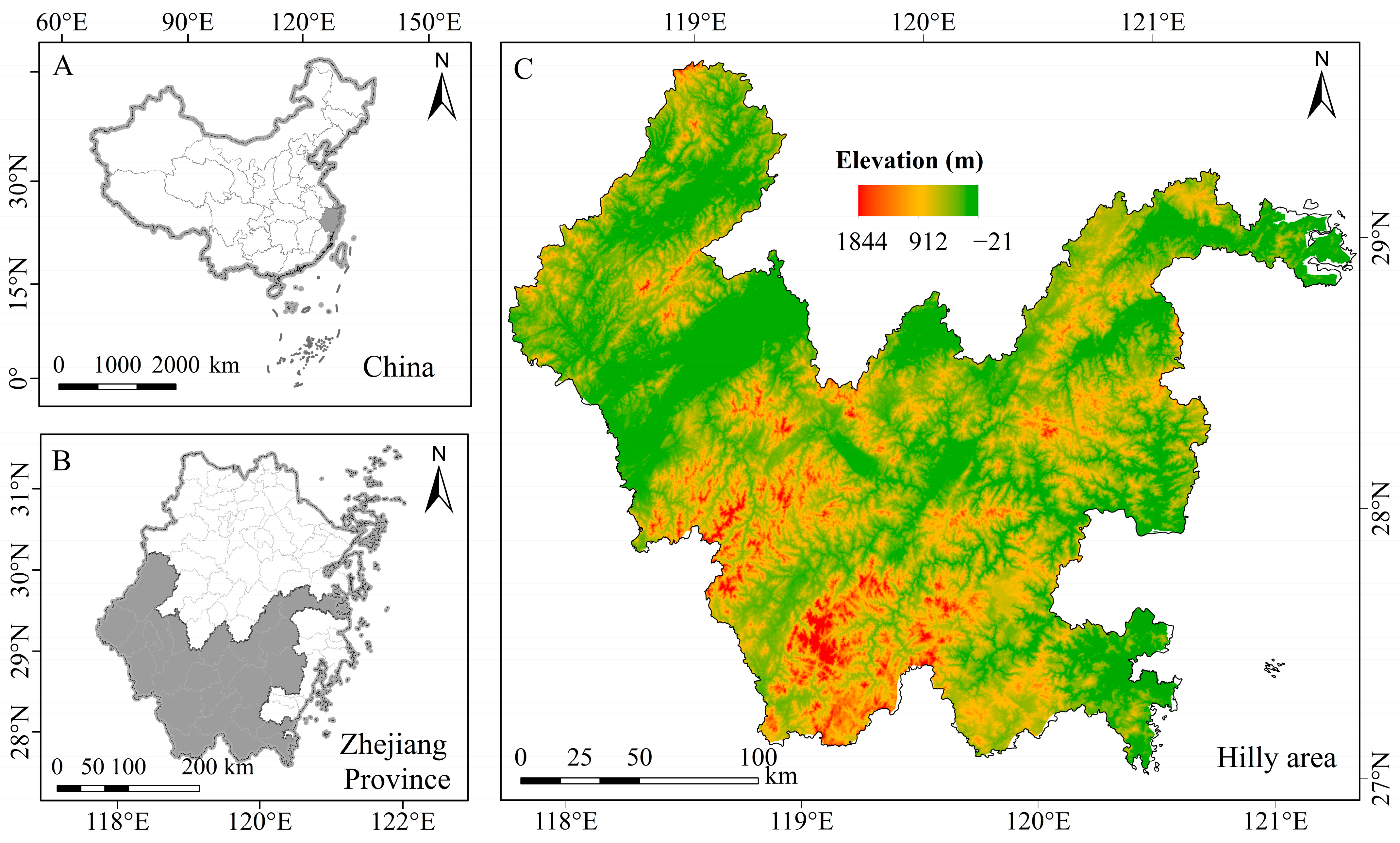
Figure 1. Study area. (A) The location of Zhejiang Province in China; (B) The location of the study area in Zhejiang Province; (C) DEM of study area. Note: This figure was created based on the standard map of China (Approval No. GS(2019)1822) downloaded from the Standard Map Service website of the Ministry of Natural Resources of China. No modifications were made to the base map, and this applies to all subsequent figures.
Land 14 01766 g001
Figure 2. Distribution pattern of land use (2000–2020).
Land 14 01766 g002
Figure 3. Characteristics of land use transformation (2000–2020). Notes: 1: CL; 2: FL; 3: GL; 4: WB; 5: BL, 6: UL.
Land 14 01766 g003
Figure 4. The center of gravity transfer of land use (2000–2020). Notes: LD: Liandu; WY: Wuyi; JY: Jinyuan; SY: Songyang.
Land 14 01766 g004
Figure 5. Distribution of EEQI (2000–2020). (A) EEQI in 2000; (B) EEQI in 2010; (C) EEQI in 2020; (D) The overall EEQI for the study area.
Land 14 01766 g005
Figure 6. Hot spots of EEQI (2000–2020).
Land 14 01766 g006
Figure 7. The performances of XGBoost-SHAP model.
Land 14 01766 g007
Figure 8. SHAP feature summary and relative importance of driving factors (2000–2020).
Land 14 01766 g008
Figure 9. Partial dependence plot of driving factors on EEQ (2000–2020). (A) ELF; (B) SLP; (C) ASP; (D) TMP; (E) NDVI; (F) GDP; (G) PD; (H) RD.
Land 14 01766 g009
Figure 10. Interaction of driving factors. (A) SHAP interaction summary plot; (B) Interaction effects among factors.
Land 14 01766 g010
Figure 11. The interaction between NDVI and other factors. (A) ELF; (B) SLP; (C) ASP; (D) TMP; (E) GDP; (F) PD; (G) RD.
Land 14 01766 g011
Table 1. EEQI weight of every land use category.
Land Use CategorySecondary ClassificationEEQI Weight
CLPaddy field0.30
Dry land0.25
FLForest0.95
Scrubland0.65
Sparse forest0.45
Other forest0.40
GLHigh coverage grassland0.75
Medium coverage grassland0.45
Low coverage grassland0.20
WBInland waterway0.55
Natural lake0.75
Artificial water0.55
Intertidal flat0.45
Floodplain0.55
BLUrban land0.20
Rural residential area0.20
Other construction land0.15
ULMarshland0.65
Bare soil0.05
Bare rock0.01
Table 2. Driving factors of EEQ.
TypeFactorsAbbreviationVIF
Natural factorsElevationELV1.627
SlopeSLP1.629
AspectASP1.034
TemperatureTMP1.414
NDVINDVI1.449
Socioeconomic factorsPer capita GDPGDP1.340
Population densityPD1.323
Road densityRD1.021
Table 3. Land use transfer matrix at each stage (Unit: km2).
YearsTypeCLFLGLWBBLULLoss
2000–2010CL6038.33 175.02 7.63 83.18 349.86 0.11 615.80
FL280.19 35,716.31 100.97 69.76 203.93 2.86 657.70
GL6.54 74.60 1035.91 2.17 14.45 0.51 98.28
WB10.65 10.64 1.97 796.51 7.52 0.07 30.84
BL8.34 3.80 0.18 1.33 336.23 0.00 13.65
UL0.04 2.10 1.54 0.42 0.68 18.99 4.79
Gain305.77 266.16 112.29 156.85 576.44 3.55 1421.06
2010–2020CL6191.00 0.27 1.14 152.71 154.12
FL 35,748.60 6.36 0.74 232.47 239.57
GL 3.65 1130.49 14.98 18.63
WB 949.90 20.99 20.99
BL0.25 4.01 13.55 0.46 895.25 18.26
UL 0.60 21.95 0.60
Gain0.25 7.66 20.18 2.34 421.76 0.00 452.18
2000–2020CL5888.73 172.02 7.79 84.23 501.24 0.11 765.39
FL276.80 35,488.81 114.57 70.50 420.50 2.84 885.20
GL6.30 74.13 1023.77 1.98 27.49 0.51 110.41
WB10.44 10.19 1.97 790.95 13.74 0.07 36.41
BL7.92 3.55 0.10 1.33 336.97 12.92
UL0.04 2.09 1.54 0.42 1.28 18.42 5.37
Gain301.50 261.98 125.98 158.46 964.25 3.53 1815.70
Disclaimer/Publisher’s Note: The statements, opinions and data contained in all publications are solely those of the individual author(s) and contributor(s) and not of MDPI and/or the editor(s). MDPI and/or the editor(s) disclaim responsibility for any injury to people or property resulting from any ideas, methods, instructions or products referred to in the content.