Article

Monitoring Spatiotemporal Dynamics of Farmland Abandonment and Recultivation Using Phenological Metrics

1
Institute of Geographic Sciences and Natural Resources Research, Chinese Academy of Sciences, Beijing 100101, China
2
College of Resource and Environment, University of Chinese Academy of Sciences, Beijing 100049, China
3
State Key Laboratory of Remote Sensing and Digital Earth, Aerospace Information Research Institute, Chinese Academy of Sciences, Beijing 100194, China
4
Business School, Beijing Technology and Business University, Beijing 100048, China
5
Institute for Cultural and Tourism Development, Beijing Technology and Business University, Beijing 100048, China
*
Author to whom correspondence should be addressed.
Land 2025, 14(9), 1745; https://doi.org/10.3390/land14091745
Submission received: 21 July 2025 / Revised: 26 August 2025 / Accepted: 26 August 2025 / Published: 28 August 2025
(This article belongs to the Special Issue Connections Between Land Use, Land Policies, and Food Systems)

Abstract

Driven by both natural and anthropogenic factors, farmland abandonment and recultivation constitute complex and widespread global phenomena that impact the ecological environment and society. In the Inner Mongolia Yellow River Basin (IMYRB), a critical tension lies between agricultural production and ecological conservation, characterized by dynamic bidirectional transitions that hold significant implications for the harmony of human–nature relations and the advancement of ecological civilization. With the development of remote sensing, it has become possible to rapidly and accurately extract farmland changes and monitor its vegetation restoration status. However, mapping abandoned farmland presents significant challenges due to its scattered and heterogeneous distribution across diverse landscapes. Furthermore, subjectivity in questionnaire-based data collection compromises the precision of farmland abandonment monitoring. This study aims to extract crop phenological metrics, map farmland abandonment, and recultivation dynamics in the IMYRB and assess post-transition vegetation changes. We used Landsat time-series data to detect the land-use changes and vegetation responses in the IMYRB. The Farmland Abandonment and Recultivation Extraction Index (FAREI) was developed using crop phenology spectral features. Key crop-specific phenological indicators, including sprout, peak, and wilting stages, were extracted from annual MODIS NDVI data for 2020. Based on these key nodes, the Landsat data from 1999 to 2022 was employed to map farmland abandonment and recultivation. Vegetation recovery trajectories were further analyzed by the Mann–Kendall test and the Theil–Sen estimator. The results showed rewarding accuracy for farmland conversion mapping, with overall precision exceeding 79%. Driven by ecological restoration programs, rural labor migration, and soil salinization, two distinct phases of farmland abandonment were identified, 87.9 kha during 2002–2004 and 105.14 kha during 2016–2019, representing an approximate 19.6% increase. Additionally, the post-2016 surge in farmland recultivation was primarily linked to national food security policies and localized soil amelioration initiatives. Vegetation restoration trends indicate significant greening over the past two decades, with particularly significant increases observed between 2011 and 2022. In the future, more attention should be paid to the trade-off between ecological protection and food security. Overall, this study developed a novel method for monitoring farmland dynamics, offering critical insights to inform adaptive ecosystem management and advance ecological conservation and sustainable development in ecologically fragile semi-arid regions.

1. Introduction

Land-use changes show impacts on global ecosystems [1,2] and human well-being [3,4]. Among its various forms, transitions between active cultivation and land abandonment have attracted considerable attention due to their significant ecological and socioeconomic consequences [5,6]. Farmland abandonment generally refers to a gradual decline in farming intensity, resulting in underutilization and eventual cessation of cultivation, the state of land left unmanaged and idle with no expectation of future agricultural use, or the permanent conversion of farmland into unmanaged grasslands, fallow fields, scrublands, or young forests [7,8]. Conversely, recultivation refers to the reinstatement of agricultural production on previously abandoned land, which reflects dynamic human responses to evolving resource demands, market forces, or policy incentives [9,10]. These bidirectional land-use transitions create spatially heterogeneous landscapes where ecological recovery competes with food production priorities. Thus, acquisition of their spatiotemporal dynamics is critical for reconciling environmental resilience and socioeconomic stability in marginal agricultural zones.
Two primary methodologies are employed in monitoring farmland abandonment and recultivation: statistical data analysis and remote sensing techniques. The former approach typically relies on questionnaire surveys conducted among farmers [11] or official statistics [12], such as FAOSTAT, to gather information on abandoned farmland. Nevertheless, such statistical data often lacks spatial information and fails to capture dynamic changes, such as the reduction in or expansion of abandonment [13]. Furthermore, the inherent subjectivity of questionnaire distributors and surveyed farmers introduces complexities and challenges in achieving high-precision monitoring of farmland abandonment. Remote sensing offers a powerful tool for mapping the spatiotemporal dynamics of farmland conversion. Case studies have focused on regions such as Central and Eastern Europe [14,15], Africa [16], and Central Asia [17,18]. In China, abandonment and recultivation mainly focus on ecologically fragile areas, urbanization-affected regions, and agropastoral ecotones, for example, the Loess Plateau [19,20,21].
Previous studies have used various remote sensing datasets to monitor farmland abandonment and recultivation [22,23,24,25,26]. The Moderate-Resolution Imaging Spectro-radiometer (MODIS) is widely employed for large-scale analyses due to its high temporal resolution and global coverage [27,28]. However, the coarse spatial resolution of MODIS (250–500 m) causes mixed-pixel effects, where fragmented abandoned fields are spectrally blended with adjacent land covers such as cropland, grassland, or shrubland, thereby hindering precise discrimination of internal land-use changes. More recently, Sentinel-2 data, with a higher spatial resolution of 10–20 m, have been increasingly applied to detect abandonment patterns [29,30]. Nonetheless, Sentinel-2 has only been available since 2015, limiting its use for the long-term temporal analyses necessary to capture extended trends in farmland dynamics. Alternatively, sensors like Landsat TM/ETM+/OLI offer a spatial resolution of 30 m and a revisit cycle of 16 days, providing a balance between spatial detail and historical continuity. This makes Landsat series data well suited for detecting fragmented farmland changes over large regions and long time series [31,32,33].
The analysis of remote sensing images possesses noteworthy benefits in rapidly mapping the temporal and spatial extents of cropland abandonment [34,35]. One commonly employed method involves assigning categorical values to pixels [36], determining whether a specific pixel qualifies as an “abandonment pixel” or a “recultivation pixel”. However, due to the fragmented nature of abandoned farmland, accurately capturing its complete coverage across an entire pixel can be challenging [37,38]. This fragmentation poses difficulties in discerning the internal components of image elements. More time series approaches have been explored, encompassing both time-series-based classification and trajectory-based methods [39]. Despite providing valuable insights into the intricate dynamics and transitions of farmlands, these techniques grapple with the challenge of mixed pixels, which encompass contributions from diverse land cover types within individual pixels, thereby introducing inaccuracies in the process of abandonment mapping. To further enhance the precision of farmland abandonment extraction, spectral mixture analysis methods have been introduced, like the Linear Mixture Model [40]. By decomposing the spectral signatures of pixels into their constituent components, it enables the identification of sub-pixel farmland abandonment. Nevertheless, in small and steep areas, the selection of appropriate end members remains a formidable task.
Phenological information derived from time-series remote sensing data has become an effective approach for identifying farmland abandonment due to its ability to capture temporal changes in vegetation growth cycles. By analyzing vegetation indices such as NDVI across the growing season, researchers can distinguish abandoned farmland, which typically exhibits altered or delayed phenological patterns compared to actively cultivated fields [41,42]. This method has been successfully applied in various regions, including temperate and semi-arid zones, to monitor abandonment and subsequent natural vegetation succession [43]. Moreover, phenology-based approaches facilitate differentiation between cropland and other land covers, improving classification accuracy [44]. However, the temporal resolution of the remote sensing data limits the precision of phenological metrics; for example, sensors with coarse revisit intervals may miss critical growth stages [45]. This limitation can be addressed by fusing data from multiple sensors with complementary temporal and spatial resolutions, such as combining MODIS with Landsat or Sentinel-2. Additionally, advanced interpolation algorithms, such as the Savitzky–Golay filter [46], can reconstruct continuous vegetation growth curves from sparse observations, reducing the impact of infrequent data acquisition on phenological metric extraction.
Farmland transitions are influenced by a complex interplay of natural, socioeconomic, and institutional variables. Many studies have highlighted that the biophysical environment, such as slope, soil quality, climate variability, and water availability, played a foundational role in shaping land suitability and abandonment risk [47]. For instance, steep terrain and low soil fertility are consistently linked with higher abandonment probability in both mountainous and arid regions. On the socioeconomic side, population aging, labor migration, rising off-farm employment opportunities, and land marginalization due to urbanization are frequently cited as key drivers of abandonment in rural areas [48,49,50]. In many regions, the decline in rural labor and the rising opportunity cost of farming have led to widespread underuse of agricultural land, especially in remote or economically less competitive zones [51,52,53]. Conversely, recultivation is often influenced by land policy interventions (e.g., land consolidation and subsidies), market incentives (e.g., crop price fluctuations), and improvements in agricultural technology and infrastructure [54]. In China, recent studies also emphasize the importance of institutional and policy frameworks, such as tenure security, land transfer mechanisms, and ecological compensation, in mediating abandonment and recultivation behaviors [55]. The interaction of these factors varies significantly across regions and scales.
Thus, to address critical gaps, this study takes the IMYRB as the research area and conducts a whole-chain analysis of bidirectional land use transitions (Figure 1). First, based on the phenological key nodes, we developed an extraction model to monitor farmland abandonment and recultivation and mapped their spatiotemporal distributions. Building on this, we tracked vegetation dynamics across these transition zones. Subsequently, we performed an in-depth analysis of the drivers underlying both land transitions and vegetation changes in abandoned, recultivated areas. Finally, we outline the adaptive responses required to mitigate resultant ecological impacts and guide future land management. Focusing on 1999–2022, this study pursues four integrated objectives.
(1)
Develop a framework to extract crop-specific phenological metrics from NDVI time-series data for major crops.
(2)
Map 1999–2022 spatiotemporal dynamics of farmland abandonment and recultivation, identify key temporal patterns and hotspots, and analyze policy and socio-economic drivers.
(3)
Evaluate vegetation recovery and degradation risks after land-use transitions. Monitor vegetation dynamics in transition zones to evaluate post-transition recovery trends and degradation risks
(4)
Explore trade-offs between ecological protection goals and food security implications and propose adaptive strategies for sustainable land management.
This study aims to provide novel insights into the mechanisms governing farmland conversion in ecologically vulnerable regions and offer practical guidance for balancing ecological restoration with agricultural sustainability. Beyond regional relevance, its findings hold global value: the phenology-based approach to tracking farmland transitions is adaptable to fragile agricultural systems worldwide, while the clarified ecological trade-offs and scalable strategies for reconciling ecology and food security contribute to advancing SDG goals.

2. Materials and Methods

2.1. Study Area

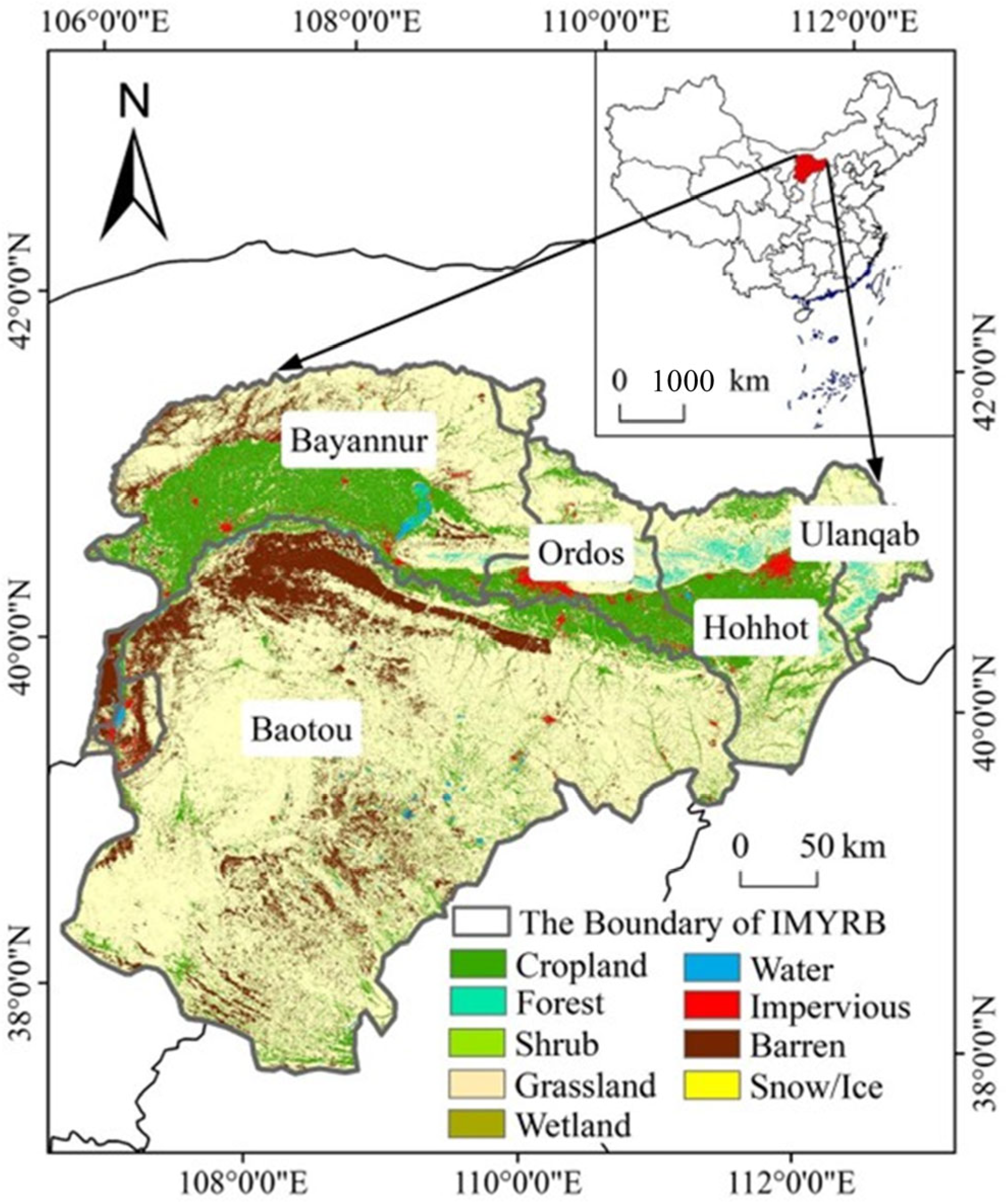
The Inner Mongolia section of the Yellow River Basin (IMYRB), situated at the northernmost tip of the Yellow River Basin, spans from 38°26′ N to 42°50′ N in latitude and 106°59′ E to 110°10′ E in longitude (Figure 2). This region encompasses multiple cities, including Alxa League, Wuhai City, Ordos, Baotou, and Hohhot, with a river course length of 843.5 km and a drainage area of 15,100 km2. IMYRB is not only an ecologically fragile area but also a key area for food security. On the one hand, due to natural factors such as an arid climate, uneven precipitation, and increasing human activities, the ecosystems in the IMYRB were severely degraded and showed vulnerability [56]. The Grain for Green (GFG) Program has been pivotal in ecological restoration in IMYRB, with the result that a significant amount of slope farmland has subsequently withdrawn from agricultural use. On the other hand, since the 2012 18th Party Congress, China has heightened its focus on food security, prioritizing stable grain production and arable land protection. As a key agricultural region, the IMYRB has adopted strict measures to prevent the non-agricultural conversion of farmland and improve cultivable land utilization.

2.2. Data

This study was conducted using various data (Table 1), including MODIS NDVI product, Landsat NDVI images, topography data, and validation data. Among this dataset, the MODIS NDVI product was processed to reveal the phenological rules, Landsat NDVI images were as the primary input to monitor the farmland and vegetation restoration, the topographical information was taken into account to enhance the accuracy of identifying farmland, and the validation was conducted at the spatial sampling sites.

2.2.1. MODIS NDVI Product

The time-series NDVI data is capable of revealing underlying attributes of farmland. In this study, the MOD13Q1, a MODIS NDVI product with a 16-day time composition and a spatial resolution of 250 m, was used to analyze crop phenological metrics (the sprouting period, utmost luxuriance period, and withering period) and vegetation restoration trends. Owing to the wide usage and high-frequency updating for MODIS products, well-designed data search platforms and auxiliary tools come into application [58]. The MOD13Q1 dataset was acquired from the EarthData system. The MODIS reprojection tool (MRT) was utilized to mosaic individual tiles and unify the map projection for consolidating the composite dataset in further analysis [59].

2.2.2. Landsat Images

After identifying the crop phenological metrics using MODIS data, Landsat images on specific phenological key periods were used for farmland conversion monitoring. Data acquisition and preprocessing were performed using Google Earth Engine (GEE) [60,61]. Landsat 5 imagery was used for the period 1999–2012, while Landsat 8 data covered 2013–2022. The processing of the Landsat dataset involved three main steps: cloud removal, NDVI calculation, and generation of gap-free images. First, cloud-contaminated pixels were removed. Second, by deriving land surface reflectance (LSR) in red and near-infrared (NIR) channels, the NDVI images for Landsat were calculated as follows:
μ i = ρ N I R , i ρ R e d , i ρ N I R , i + ρ R e d , i    
where the μ i is the calculated NDVI value for pixel i and ρ N I R , i and ρ R e d , i are the values of LSR for NIR and red channels, respectively.
Third, for each phenological key stage—namely the sprouting period, utmost luxuriance period, and withering period—Landsat NDVI images were generated using a five-year temporal sliding window. Within this window, missing NDVI values were filled based on the following three rules:
(1)
If the number of effective values was more than two, missing values were estimated using temporal linear interpolation.
(2)
If only one valid observation was present, its value was directly assigned to the missing pixel.
(3)
If no valid observations existed, the missing value was filled in using MOD13Q1 NDVI data from the temporally and spatially closest date. To ensure compatibility, the MOD13Q1 product was resampled to 30 m using bilinear interpolation prior to gap filling.

2.2.3. Topography Information

Topographic factors play a critical role in farmland changes [62]. Therefore, the SRTMGL1_003 digital elevation model (DEM) product was used to analyze the abandonment and recultivation, which was also derived from the GEE platform.

2.2.4. Sampling and Validation Data

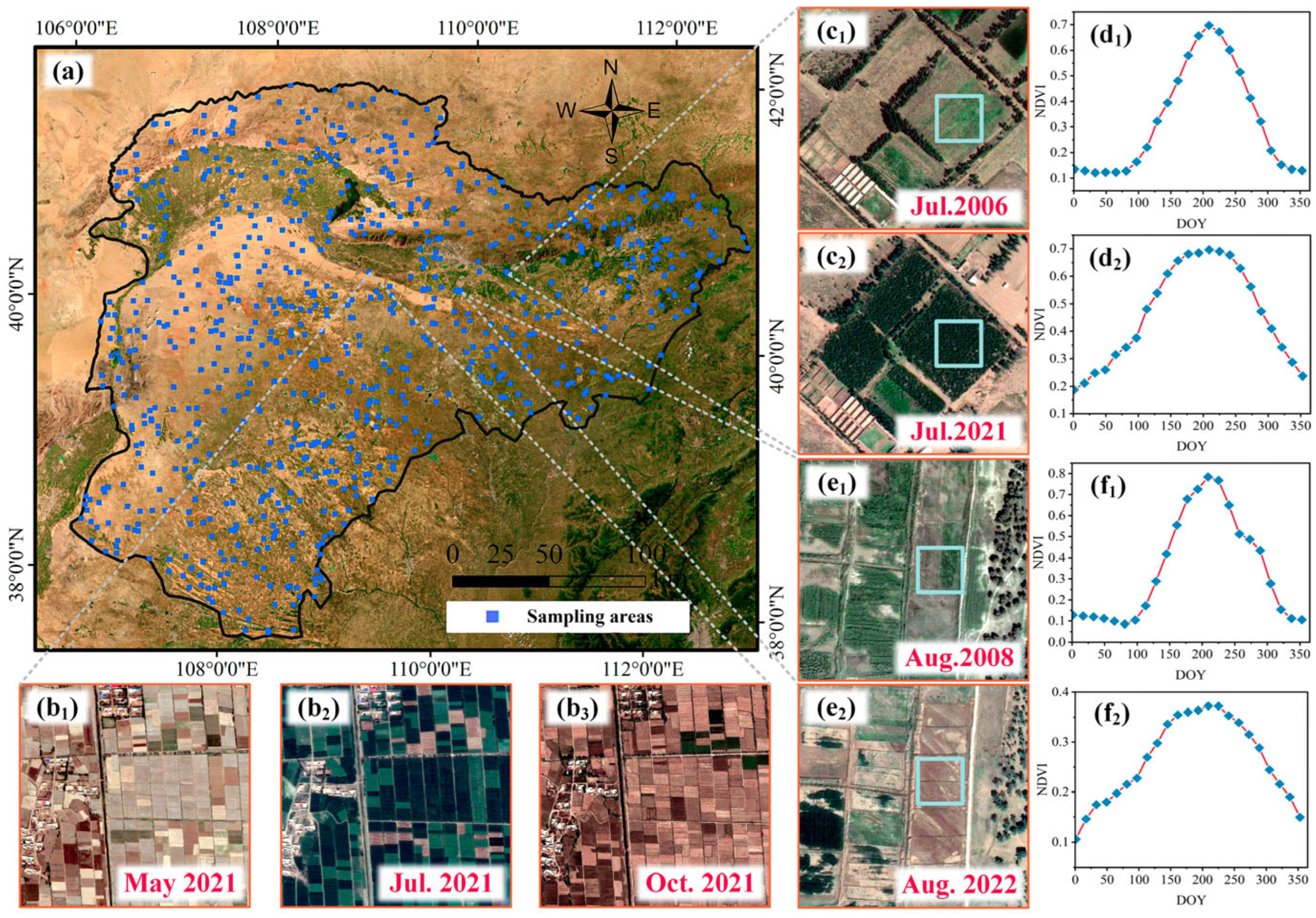
To ensure robust land cover classification and change detection, sampling and validation tend to rely on high-resolution imagery from Google Earth [63,64,65,66]. A total of 700 samples were generated randomly across the IMYRB (Figure 3a). For phenological and farmland dynamic monitoring, 100 random samples were selected to extract phenological metrics. Through visual interpretation and temporal analysis, key crop phenological stages were identified: sprouting in May, the utmost luxuriance period around July, and withering in October (Figure 3(b1–b3)). Sixty samples were used for active farmland analysis, and one hundred samples were selected to detect the abandonment and recultivation extent at the pixel level.
For validation, 200 samples were randomly employed to validate farmland using agricultural features in Google Earth imagery, including regular grid patterns, linear field boundaries, and seasonal vegetation dynamics (e.g., bare soil in fallow periods, greenness during growth, and senescence in October). An additional 100 samples were used to evaluate abandonment and recultivation. In this study, abandonment was defined as areas historically identified as farmland showing no crop cultivation in the study year and its preceding/following years or conversion to plantations. Recultivation was classified as non-cropland areas that exhibited continuous cropping for two continuous years starting from the study year.
Accuracy was further cross-checked against established land cover products (GLC30 and CLCD). Two hundred samples were generated for accuracy comparison of different products. Spectral validation involved comparing NDVI trajectories between farmland, forest, and bare land to characterize temporal dynamics (Figure 3(c1–f2)).

2.3. Methods

2.3.1. Time-Series NDVI Curve Smoothing

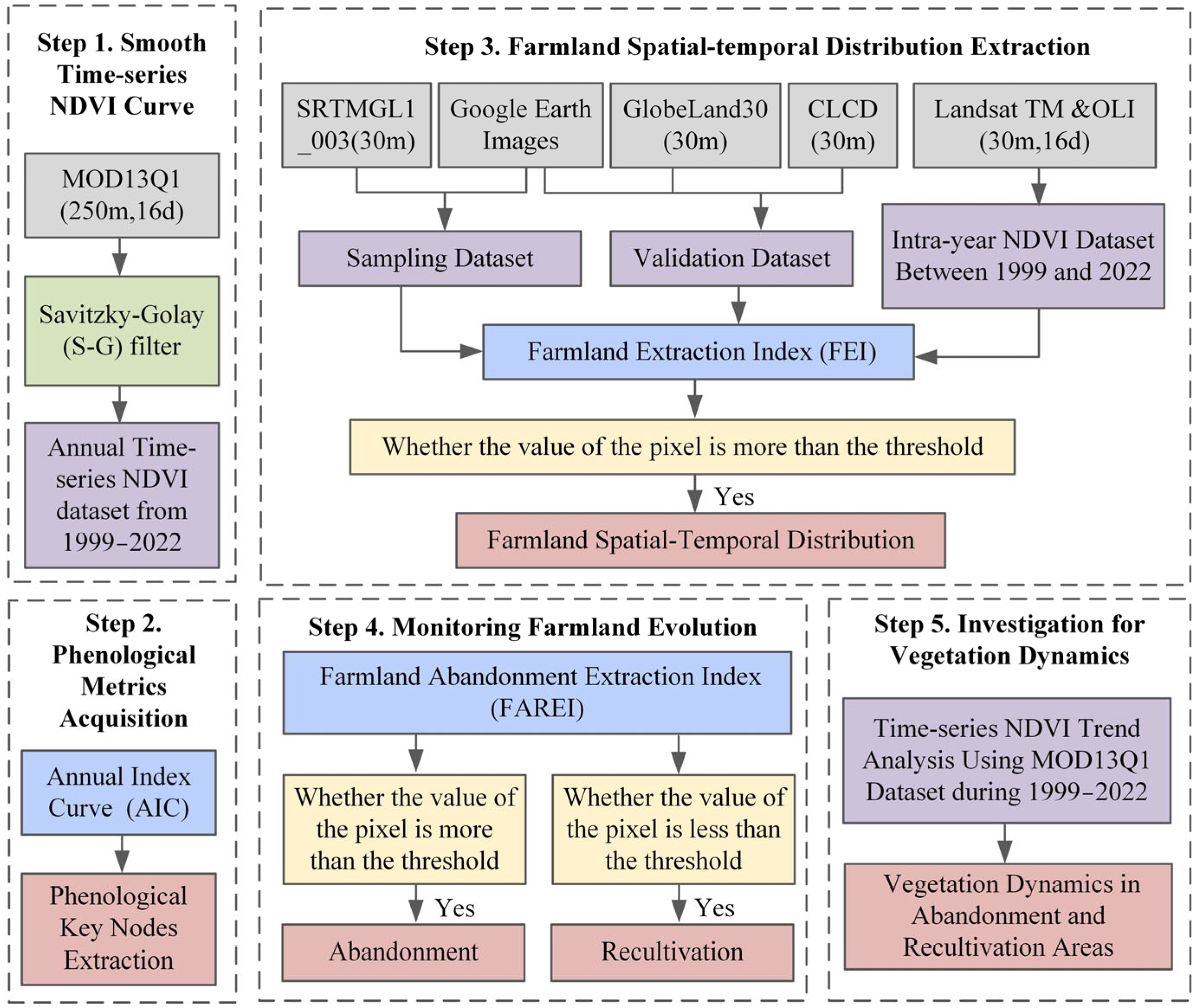
We proposed a framework for abandonment and recultivation extraction and vegetation response monitoring (Figure 4). In order to capture plain evolution trends of crop conditions, the Savitzky–Golay (S–G) filter was applied to smooth time-series NDVI curves. The S–G filter, a signal convolution algorithm with least squares estimation, can suppress the outliers in NDVI curves [67]. This algorithm is as follows.
μ k s m o o t h = 1 M i = m m C i μ k + i k H ,   k N +
where k and i represent the positions in NDVI curve and the window of the filter, respectively; μ k + i and μ k s m o o t h are original and smoothed NDVI, respectively; C i is the fitted coefficient; H is the length of the NDVI curve; the window size of this filter is expressed as N = 2 m + 1 ; and N is than H to meet the demand for least square fitting.

2.3.2. Phenological Metric Acquisition

Analyzing phenological indicators helps to understand crop growth patterns [68]. In the IMYRB, four typical crops (i.e., spring wheat, summer maize, potato, and sunflowers) were selected to derive detailed phenological information from multi-temporal NDVI curves. Spring wheat is planted in early April and harvested from late July to early August. The growth cycle of corn is from May to September. Sunflowers and potatoes have similar growth cycles, which are between May and October [69]. Growth cycles of these crops are mainly concentrated on the period from April to October. To monitor the interannual NDVI trend and capture the temporal growth nodes of typical crops, an empirical model for the Annual Index Curve (AIC) was built, i.e.,
μ t = δ α e x p μ α s i n π ω ( t m t ) + μ 0 + δ 0 ,   t t s μ α cos π ω · t m t 365 + μ 0 ,   t > t s
where μ is NDVI at DOY t ; μ 0 is the residual NDVI at the fallow stage; μ α is the NDVI amplitude; ω is the period of this model; t m is the DOY of the maximum NDVI; t s   is the DOY when NDVI begins to mutate; and δ α and δ 0 are the gain and offset at the fallow stage.

2.3.3. Farmland Extraction and Abandonment/Recultivation Monitoring

Crops exhibit distinct NDVI variations across growth stages, with marked differences between sprouting (Spr), utmost luxuriance (UL), and withering (Wit) periods—these effectively distinguish farmland from other land cover types [70]. In this study, the Farmland Extraction Index (FEI) was set as the core indicator for farmland extraction, which lays the foundation for subsequent statistics of abandoned and recultivated lands. The FEI can be expressed as follows.
F E I i = μ i U L μ i S p r + μ i U L μ i W i t = 2 × μ i U L ( μ i S p r + μ i W i t )
where F E I i is the farmland extraction index of pixel i and μ i S p r , μ i U L , and μ i W i t are the NDVI at sprouting, utmost luxuriance, and withering nodes, respectively.
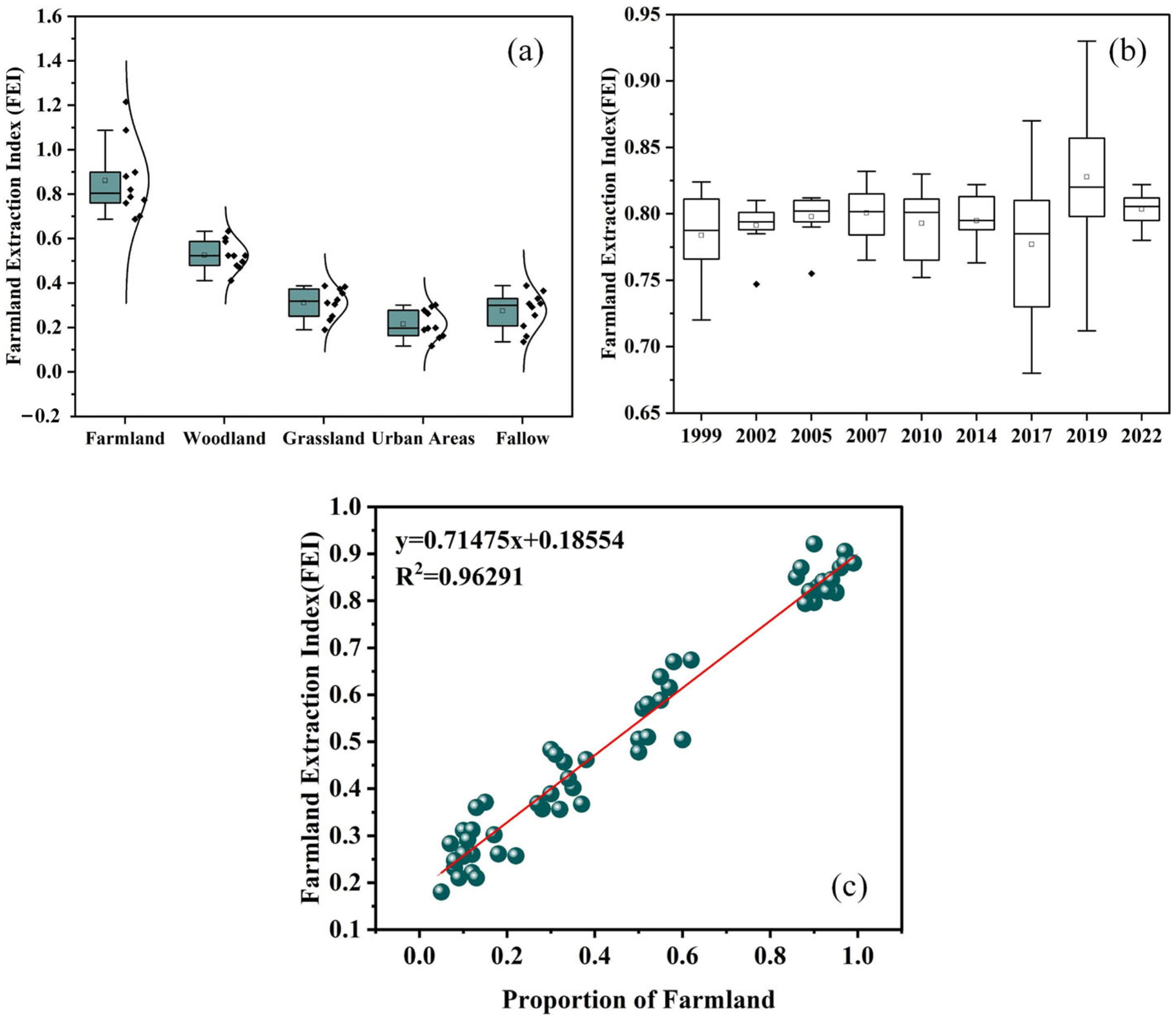
The farmland FEIs are valued from 0.68 to 1.22, and for woodland, grassland, urban area, and fallow, the FEIs are below 0.66 (Figure 5a). We also considered the temporal distribution of FEI. FEI values for farmland remained consistently above 0.72 from 1999 to 2022 (Figure 5b). However, many pixels may cover at least two types of surfaces, resulting in the occurrence of mixed pixels [71]. The correlation between FEI and the farmland proportion within Landsat pixels was monitored. A pixel with crop coverage exceeding 50% was defined as farmland [39,72]. To determine the threshold for active farmland identification, a total of 60 sample pixels with varying proportions of cropland were selected (Figure 5c). By analyzing the relationship between FEI values and the corresponding farmland proportions, a clear positive correlation was observed (R2 = 0.96291). The FEI threshold was identified as 0.54 for distinguishing active farmland.
FEI works because farmland crops have significantly higher NDVI in UL than in sprouting (Spr) and withering (Wit) stages—a pattern less pronounced in natural vegetation (e.g., grasslands, woodlands) or non-cultivated land, whose phenological curves show smaller variations. Thus, higher FEI values indicate a greater likelihood of farmland.
To monitor farmland abandonment and recultivation, we developed the Farmland Abandonment and Recultivation Extraction Index (FAREI) as the key indicator for quantifying farmland status transitions.
F A R E I i = F E I i N + 1 F E I i N
where F A R E I i is the index to indicate farmland variation in pixel i and F E I i N + 1 and F E I i N are the value of FEI for N and   N + 1 years, respectively.
FAREI captures shifts in farmland status through the difference between FEI in the previous year (N) and the subsequent year (N + 1) using the phenological differences between farmland and non-farmland vegetation. When farmland is abandoned, crops tend to be replaced by natural vegetation (e.g., weeds). This reduces NDVI peaks and narrows growth-stage differences, lowering FEI in year N + 1 compared to year N, resulting in a positive FAREI. Conversely, during recultivation, natural vegetation is replaced by crops, restoring the distinct NDVI curve and increasing the FEI in year N + 1 relative to year N, resulting in a negative FAREI value.
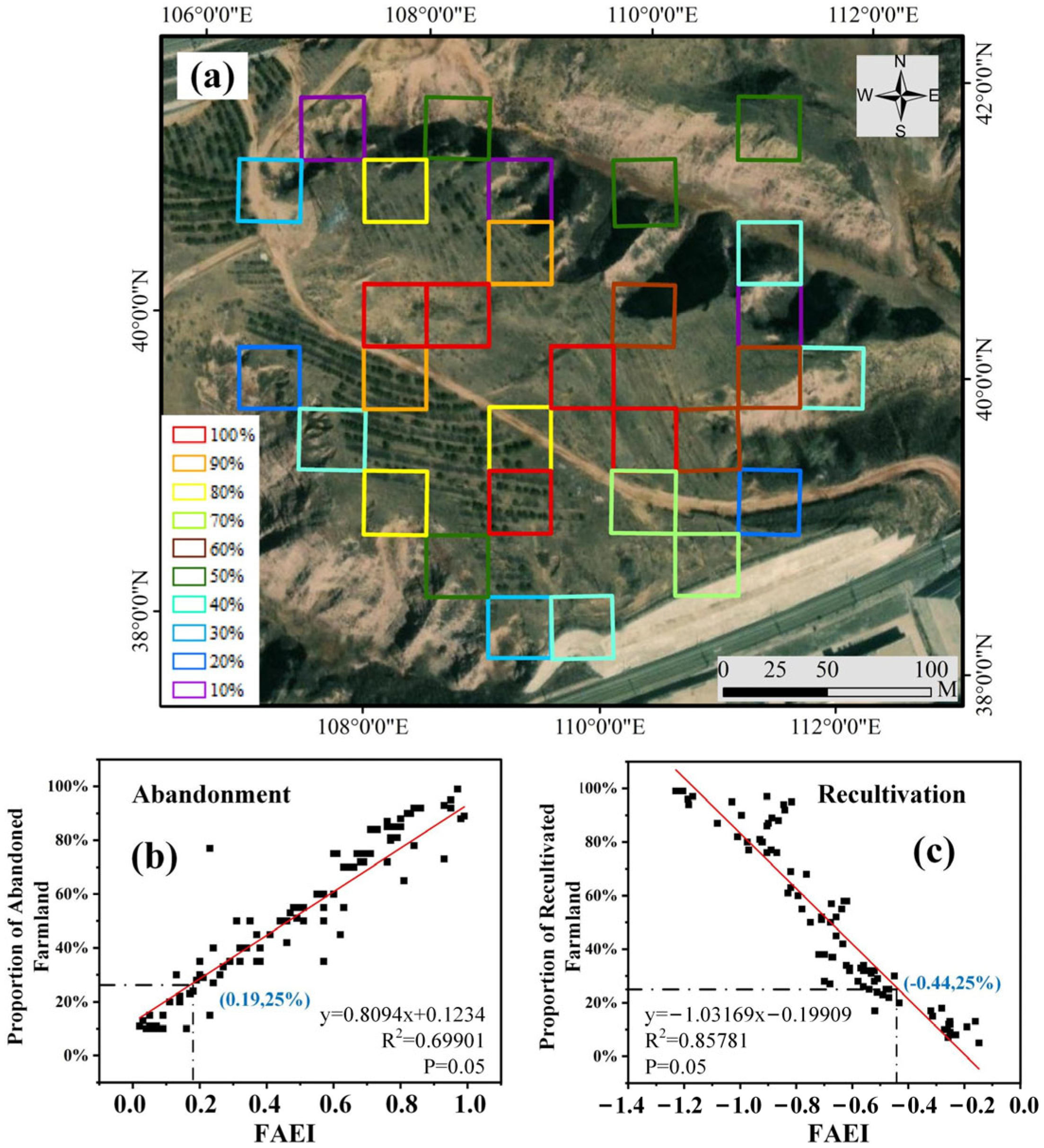
To determine the threshold for farmland abandonment and recultivation extraction, 100 samples were selected for each category. Following the approach of previous studies [39], a pixel was defined as abandoned or recultivated if the proportion of crop components decreased or increased by at least 25%, respectively. Based on the distribution of FAREI values derived from these samples, the abandonment and recultivation thresholds were determined to be 0.19 and −0.44, respectively (Figure 6).
Compared to traditional methods such as post-classification comparison, FAREI offers several advantages. It avoids subjective threshold setting and detects subtle early changes, including initial abandonment transitions. Additionally, it enables large-scale, long-term monitoring through straightforward derivation from time-series NDVI data. The effectiveness of FAREI depends on consistent phenological differences between crops and non-crop vegetation.

2.3.4. Investigation for Vegetation Restoration

The degree of vegetation restoration is a vital indicator to assess the farmland’s ecological condition [71,73]. This study integrated the Theil–Sen estimator and the Mann–Kendall test to explore the extent of vegetation restoration evolution dynamics in the abandonment and recultivation area [74,75,76]. To monitor vegetation restoration trends, the Theil–Sen estimator was employed as follows:
Q = M e d i a n μ b μ a b a ,   b > a
where M e d i a n   means the median of a sequence and μ b and μ a are the NDVI at nodes a and b , respectively. A positive Sen’s slope value (Q > 0) denotes an increasing trend in the time series, indicating vegetation restoration. Conversely, a negative Sen’s slope value (Q < 0) signifies a decreasing trend, representing vegetation degradation.
To evaluate the significance level of Sen’s slope, we first constructed the statistic S :
S = a = 1 n 1 b = a + 1 n S i g n ( μ b μ a )
where S is the value of statistics for each pixel; μ a and μ b are NDVI values at period a and b , respectively; n is the number of temporal nodes; and the Sign function is defined as
S i g n μ b μ a = + 1 ,   μ b > μ a 0 ,   μ b = μ a 1 ,   μ b < μ a
Then, we calculated the MK-Z value as follows:
Z = S 1 δ ( S ) ,   S > 0 0 ,   S = 0 S + 1 δ ( S ) ,   S < 0
in which
δ S = 1 18 n ( n 1 ) ( 2 n + 5 ) j = 1 m q j ( q j 1 ) ( 2 q j + 5 )
where n refers to the size of the time series; m is the number of tie groups, which means the subsets composed of a certain repeating element in a time-series NDVI sequence; and q j is the size of the tie group for element j . If the Z value is greater than 1.96, the trend of the time series is significant at a 95% confidence level. To evaluate vegetation changes in farmland conversion zones, we defined vegetation restoration as significant NDVI increases (Q > 0, Z > 1.96) and degradation as significant NDVI decreases (Q < 0, Z > 1.96) for both abandonment and recultivation areas.

2.4. Model Sensitivity Analysis

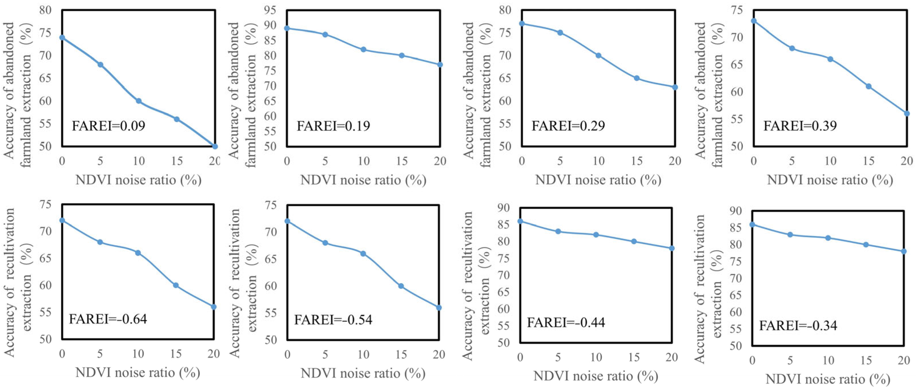
To evaluate the robustness of our farmland extraction framework, we performed model sensitivity analysis (Figure 7). Focusing on the optimal FAREI thresholds (0.19 for abandoned and −0.44 for recultivated farmland), we validated with 50 samples each. For abandoned farmland, we tested FAREI values of 0.09, 0.19, 0.29, and 0.39; for recultivated farmland, we tested FAREI values of −0.64, −0.54, −0.44, and −0.34. With NDVI noise gradients (0–20%) simulating data uncertainties, results showed that 0.19 and −0.44 outperformed neighboring values across noise levels. At 0% noise, they achieved 85% accuracy; even at 20% noise, their accuracies (77% for 0.19, 78% for −0.44) remained higher. These thresholds balance spectral differentiation, minimizing misclassification and proving robust to data variability, validating their reliability for farmland dynamics detection from remote sensing.

3. Results

3.1. Phenological Information Acquisition

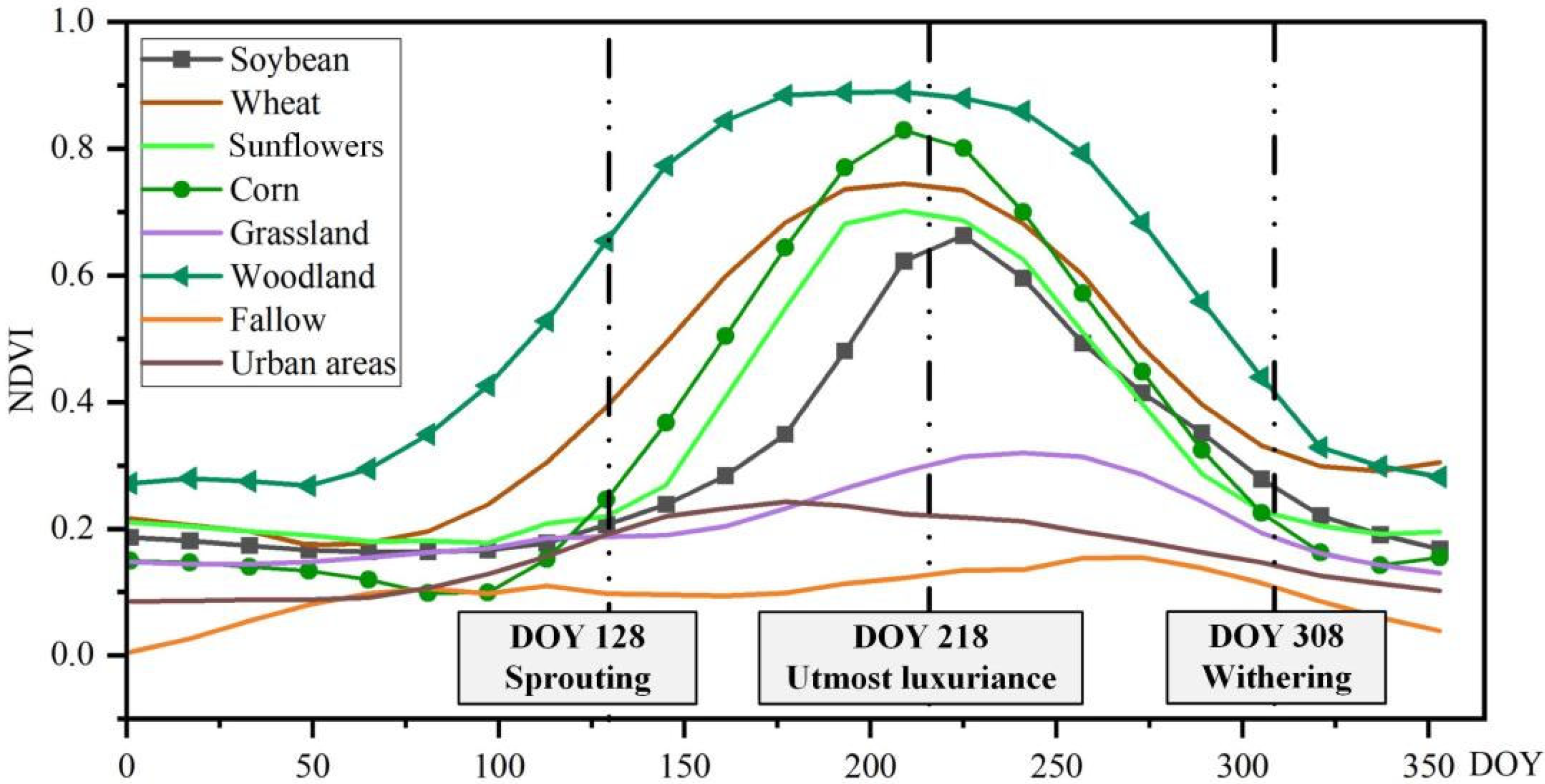
The temporally phenological characteristics usually refer to the node when the growth conditions of crops change significantly [68]. At the sprouting, utmost luxuriance, and withering stages of crops, three nodes were defined as the phenological metrics to recognize farmland. The coefficients of AIC were identified (Table 2). Based on the fitted coefficients of AIC, the values assigned to sprouting and utmost luxuriance nodes are t s (DOY 128) and t m (DOY 218), respectively; the μ ( t ) at the withering node is DOY 308. The interannual NDVI curves for various surface types were mapped for further phenological analysis (Figure 8). The NDVI curve of crops is significantly different from those of other land surface types, which demonstrates the effectiveness of time-series NDVI in capturing the phenological characteristics of farmland.

3.2. Accuracy Validation of Active Farmland, Abandonment, and Recultivation Extraction

The accuracy validation was performed using the 200, 200, and 100 sample points selected in Section 2.2.4, which were, respectively, used to verify the extraction accuracy of active farmland, different land use products, and farmland abandonment and recultivation. Validation of the Farmland Extraction Index (FEI) yielded high accuracy. Specifically, active farmland maps achieved an overall accuracy (OA) of 89.27~92.67%, with a user’s accuracy (UA) of 89.67~93.63% and a producer’s accuracy (PA) of 88.55~95.19% (Table 3). We compared the 2020 extraction results with CLCD and GLC30 data. FEI outperformed existing products with PA of 91.33%, UA of 94.48%, and OA of 89.50% (Table 4). For abandoned farmland, the Farmland Abandonment Extraction Index (FAREI) achieved peak OA of 91%, with a PA (78~94%) and a UA (79.59~91.84%) across temporal scales (Table 5).

3.3. Mapping Farmland Abandonment and Recultivation

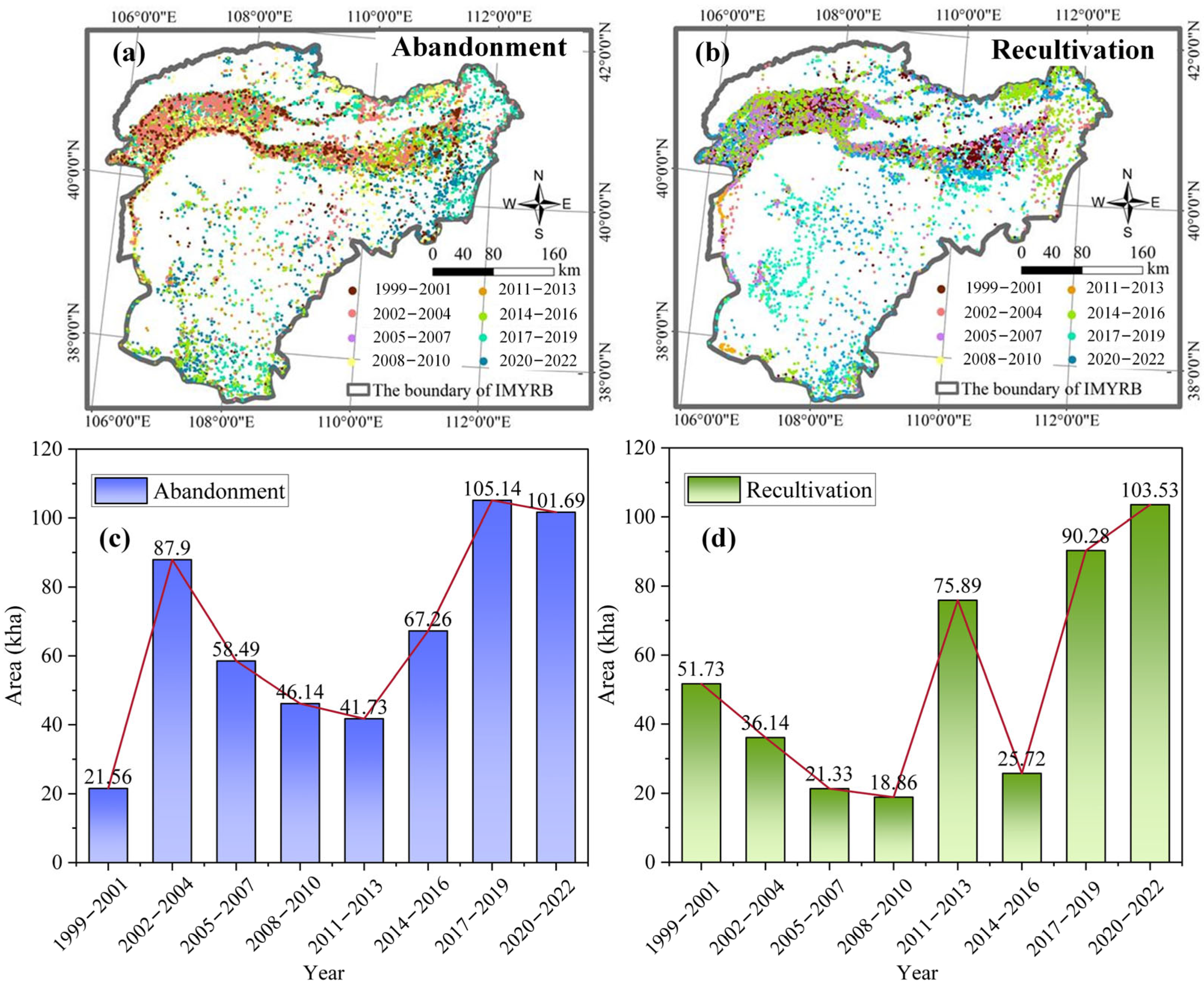
Using FAREI, the spatiotemporal patterns of farmland abandonment and recultivation in the IMYRB from 1999 to 2022 were mapped, and their areal dynamics were quantified. Spatially, abandonment and recultivation exhibited distinct temporal clustering (Figure 9a,b). Earlier phases were concentrated in the Hetao Irrigation District—an area dominated by corn, spring wheat, and sunflower cultivation due to irrigation advantages [77]. This spatial clustering likely reflects crop-specific responses. Corn (high water/management demands) was vulnerable to early ecological policy shifts (e.g., the GFG program), driving abandonment in this core irrigation zone. Sunflowers, though less water-intensive than corn, rely on stable market demand for oil. Early policy focus on ecology over economics may have reduced farmer incentives, contributing to subtle abandonment trends in sunflower-dominated plots. Meanwhile, later expansion areas align with regions where soybeans and minor crops are common; their lower resource dependence but higher sensitivity to market/soil changes could explain delayed abandonment/recultivation trends.
Temporally, farmland abandonment showed a bimodal trend (Figure 9c): the initial peak (2002–2004, 87.9 kha) coincided with large-scale ecological restoration (e.g., GFG) [78]. Here, spring wheat likely drove this peak, as ecological priorities often conflict with its intensive management needs. Additionally, sunflower fields—heavily dependent on consistent irrigation and market-driven planting decisions—may have contributed: policy-induced water reallocations for ecology could have disrupted sunflower cultivation, adding to abandonment in this phase. The later surge (2016–2019, 105.14 kha) aligns with the second GFG round, potentially targeting corn-dominated fragile lands, accelerating abandonment [79]. For sunflowers, this period’s intensified ecological scrutiny (e.g., stricter land-use regulations in marginal areas) might have accelerated abandonment in non-optimal sunflower plots, compounding the overall abandonment peak. Recultivation fluctuated in response to policies (Figure 9d). Early (1999–2005) low levels correlate with ecological dominance, where water-intensive crops like corn faced recultivation barriers. The 2011–2013 surge, driven by food security policies, likely prioritized spring wheat recultivation, boosted by local incentives. During 2016–2022, high recultivation on gentle slopes aligns with soybeans, corn and sunflowers: soybeans thrive on moderate slopes with lower irrigation; corn benefits from policy support in fertile zones; sunflowers, increasingly recognized for their drought tolerance [80] and economic value (e.g., biofuel applications) [81], began reclaiming gentle, well-drained slopes—reflecting the “ecology-food security-economic crop” balance in policy design.
The concurrent rise in farmland abandonment and recultivation after 2016 reflects synergistic policy design. The 2016 second-phase GFG program expanded ecological conversion zones and increased subsidies, accelerating abandonment in fragile landscapes (e.g., steep slopes and erodible terrain). Parallel to this, the 2017 designation of “Grain Production and Important Agricultural Product Protection Zones” prioritized agricultural intensification in suitable areas, with policy and financial incentives sustaining high recultivation rates on gentle, fertile slopes. Complementing these measures, the 2016 “Irrigation District Water-Saving Reform” in the IMYRB enhanced agricultural water-use efficiency, improving recultivation viability in water-constrained regions.
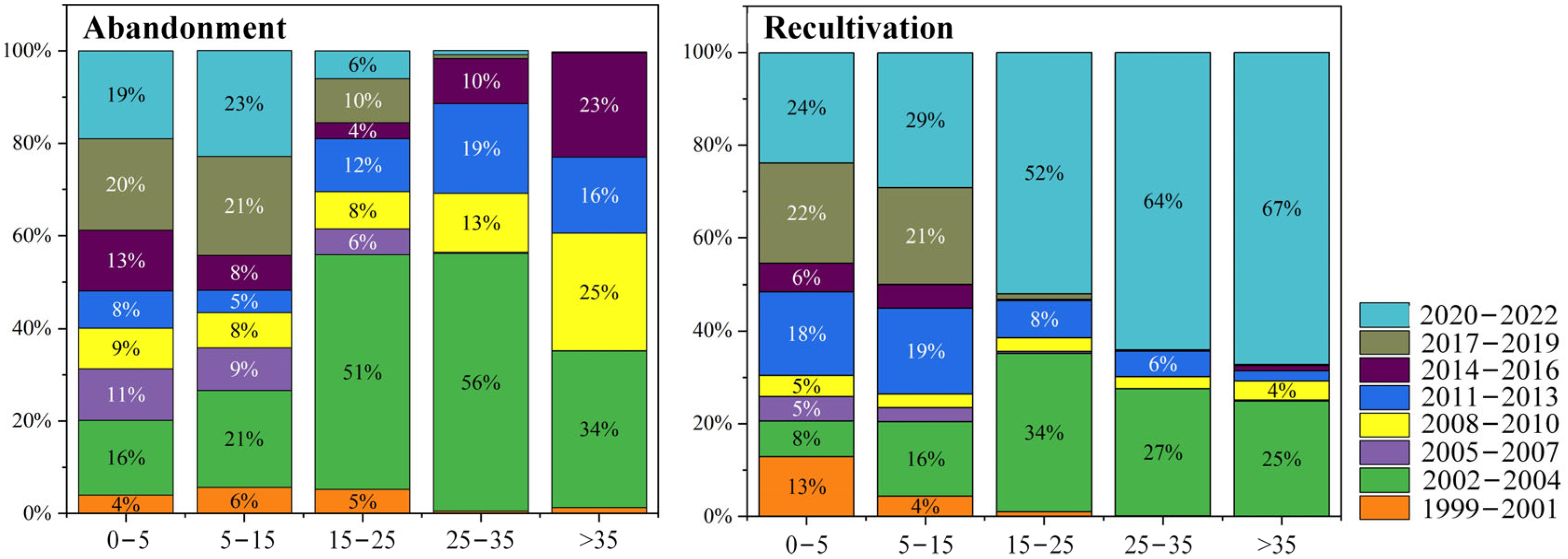
For farmland abandonment, this study found that the steeper slopes (15~25° and 25~35°) dominated the trends. Notably, 51% of abandonment occurred in the 15~25° slope class and 56% in the 25~35° class during peak periods. This result indicates that steeper terrains were more prone to abandonment, likely driven by challenges in agricultural practices (e.g., soil erosion, low productivity) and policy initiatives such as the GFG program (Figure 10). For recultivation, gentle slopes (0~5°) emerged as the primary focus, with 67% of recultivation occurring in this class during 2019–2022. Flat terrains are more conducive to farming due to easier cultivation, better water retention, and higher productivity, making them ideal for recultivation efforts aimed at boosting food security.

3.4. Monitoring Vegetation Restoration in Abandoned and Recultivated Areas

This study mapped vegetation restoration dynamics within areas of confirmed farmland abandonment or recultivation across two periods: 1999–2010 and 2011–2022 (Figure 11). Vegetation restoration is defined by NDVI trends, with distinct vegetation components: abandoned areas show restoration through natural vegetation, such as grasses, herbs, shrubs, and artificial forests planted under programs like GFG. Recultivated areas see restoration as crop growth recovery, primarily local staples such as wheat and maize, verified by Google imagery capturing crop phenology.
From 1999 to 2010, vegetation restoration covered 89.13% of conversion zones. Abandoned lands, which are characterized by natural and planted vegetation, made up 69.67% of restored areas, while recultivated lands, driven by crop growth, accounted for 30.33%. Degraded patches followed a similar pattern: 65.43% originated from abandoned lands where vegetation was stunted, and 34.57% from recultivated lands where crop growth was poor.
Between 2011 and 2022, restored areas decreased to 79.21% while degraded areas rose to 20.79%. Degraded regions shifted significantly: recultivated lands, which suffered from failed crop establishment, accounted for 73.33%, and abandoned lands, where vegetation had degraded, made up 26.67%. In restored areas, abandoned lands, which maintained persistent vegetation succession, kept a majority at 55.84%, while recultivated lands, with improved crop productivity, rose to 44.16%.

4. Discussion

4.1. Drivers of Farmland Abandonment, Recultivation, and Vegetation Dynamics

Regarding the reasons for abandonment, multiple interacting factors have contributed to the widespread fallowing of arable land in the IMYRB region. In the early 21st century, rapid urbanization and industrial expansion across northern China led to massive rural labor outmigration, as young and able-bodied workers sought better employment opportunities in urban centers, reducing the agricultural labor force and increasing the likelihood of farmland abandonment. At the same time, the implementation of large-scale ecological restoration policies, such as the Grain for Green Program (GFG) launched in 1999, led to the systematic retirement of farmland with poor soil fertility or located on steep slopes. The number of abandoned plots increased significantly during 2002–2005, marking the initial peak of GFG implementation. A second surge occurred around 2014 with the rollout of the program’s second phase (Figure 9), as part of broader national ecological rehabilitation strategies. In addition to these socioeconomic and policy-driven processes, natural environmental constraints have played an increasingly critical role. The IMYRB is situated in an arid and semi-arid climate zone and has long suffered from soil salinization, further degrading the agricultural suitability of marginal lands. Moreover, climate change has exacerbated these land-use pressures. Over the past several decades, rising temperatures in the IMYRB have intensified evapotranspiration, resulting in declining river runoff. These hydroclimatic shifts have, in turn, led to more frequent and severe drought events, collectively impairing soil moisture availability and exacerbating regional water scarcity [82,83].
Regarding the reasons for recultivation, on the one hand, our study showed that large-scale farmland abandonment posed a threat to China’s food security. In order to keep the red line of 1.8 billion mu of arable land, the 18th National Congress of China has further emphasized food security and advocated arable land recultivation. On the other hand, over the years, soil quality in irrigation areas has been improved through rational irrigation management and soil structure improvement, creating conditions for arable land reclamation.
Vegetation recovery in the IMYRB was driven primarily by large-scale ecological policies. Initiatives like GFG and the Three-North Shelter Forest Program boosted greening by establishing protective forests in erosion-prone hills and agroforestry systems in irrigated plains, particularly evident in the latter decade (2011–2022) as restored vegetation stabilized soils and improved microclimates. However, the vegetation in some areas has degraded. We analyzed the reasons for the degradation. Specifically, in the Loess Plateau, maturing GFG plantations increased soil water demand, depleting reserves and stressing drought-sensitive ecosystems [84]. Furthermore, fragmented fallow plots also posed management hurdles, especially in remote areas with limited technical support for farmers. Additionally, inadequate pest control knowledge among smallholders exacerbated vegetation decline in poorly managed sites. These trade-offs highlight the need to balance broad ecological ambitions with on-the-ground hydrological constraints and farmer capacity for long-term sustainability.

4.2. Policy Implications for Trade-Offs Between Ecological Protection and Food Security

This research found that the dual peaks of farmland abandonment and subsequent recultivation in the IMYRB region highlight the need for spatially targeted policies to balance ecological and agricultural goals. In ecologically vulnerable areas like the Loess Plateau, where soil erosion and water scarcity threaten long-term sustainability, prioritizing GFG with drought-resistant species, such as Caragana, can reduce soil moisture competition while maintaining erosion control [85]. Meanwhile, the research findings emphasize that in productive irrigation zones such as the Hetao District, fertile lands should be strictly protected under China’s arable land red line. The investments in water-efficient agriculture, including drip irrigation and salt-affected soil remediation, can help bolster food security without compromising ecological gains [86].
Additionally, this research highlights that adaptive management is critical to address the unintended consequences of large-scale interventions. For instance, the post-2016 surge in recultivation highlights the need to tie agricultural incentives to environmental outcomes. Subsidies for recultivated lands should be conditional on adopting sustainable practices like crop rotation or agroforestry, which maintain yields while delivering ecosystem benefits such as windbreaks and soil carbon sequestration. This ensures that efforts to boost food production do not undermine long-term ecological health. Furthermore, in regions where vegetation exacerbates water stress, such as the Loess Plateau, where mature forests increase soil moisture demand, shifting from water-intensive species to mixed plantings of drought-tolerant varieties can significantly reduce soil moisture stress. Such adjustments preserve key ecological functions like erosion control and carbon storage while alleviating pressure on local water resources. By tailoring interventions to specific biophysical and socioeconomic contexts, policymakers can mitigate trade-offs and foster more resilient land-use systems.
Furthermore, cross-sectoral collaboration is essential to navigate complex interdependencies. Regional monitoring platforms tracking soil salinity, vegetation health, and fallow land dynamics enable real-time policy adjustments, for example, deploying temporary fallow subsidies during droughts or reallocating ecological investments to degradation-prone areas. By integrating scientific evidence into policy design, stakeholders can transform conflicts between ecological and food security goals into synergies, ensuring sustainable land use that balances immediate needs with long-term environmental health, particularly in vulnerable regions like the IMYRB.

4.3. Robustness in Monitoring Abandonment and Recultivation Dynamics

The mapping of farmland abandonment and recultivation is crucial for effective land management and policy-making. We developed a rapid and efficient method to map abandonment and recultivation using annual Landsat time series data. Our approach utilized key phenological periods, such as growing and harvesting seasons, to simulate the proportion of cropland based on the rate of change in NDVI values. By setting appropriate thresholds, we effectively eliminated interference caused by other vegetation types, such as forests or grasslands.
Our method shows several advantages. Firstly, it requires only three images of key phenological periods, which greatly saves time and improves efficiency. Secondly, it can help reduce identification errors caused by conversion between crop types. Although the results in this study demonstrate improved classification accuracy compared to existing products, pixel-based methods remain susceptible to salt-and-pepper noise, which continues to contribute to local misclassification [87]. Such errors are particularly pronounced in areas dominated by grasslands. Thirdly, it can provide detailed spatial information at regional levels, which is critical for land managers and policymakers.
Besides, we considered that if the vegetation recovery is significantly improved after the farmland is no longer farmed, it should be due to manual intervention, such as planting artificial forests and artificial grasslands, while the areas with poor vegetation recovery tend to undergo the natural abandonment of farmland. To better understand the land use status of farmland after withdrawal from cultivation, we developed a discriminant model of cultivated land types based on vegetation restoration, using Mann–Kendall trend analysis to establish the time series and identify the type of abandoned farmland by overlaying the results with the extraction data.

4.4. Uncertainty and Limitations

First, data availability and resolution pose inherent constraints. High-quality Landsat data can be limited due to many factors, such as cloud cover, which can result in the need to use 2–3 years of data to cover the entire region. However, this introduces uncertainty into the extraction accuracy of returned farmland, as different years may have different land-use changes. To address this, future research could explore the use of higher-resolution data, such as Sentinel-2, which may provide a more accurate representation of land-use change.
Beyond data-related constraints, spatial scale limitations affect the analysis. This study only focused on mapping farmland abandonment at a regional level and did not consider local variations in the process. Future research could consider the impact of local factors, such as soil type. This could help to identify areas where farmland abandonment is most likely to occur and enable targeted interventions to prevent further abandonment.
Another key limitation lies in the classification and causal analysis of farmland transitions. This study did not distinguish between different scenarios of farmland abandonment and recultivation. For instance, abandoned land includes both land retired under ecological restoration programs and land fallowed due to socioeconomic factors, while recultivated land comprises both reclaimed fallowed land and newly cultivated natural land. Future research should classify these types more explicitly to enhance understanding of land-use trajectories. In addition, the analysis of driving factors was primarily qualitative. Thus, further studies are needed to conduct quantitative assessments of the key determinants influencing farmland transitions [1].
Additionally, the analysis overlooked crop-specific dynamics in farmland transitions. This study focused on general farmland bidirectional transitions without differentiating specific crop types in analyzing abandonment and recultivation. We fully recognize the value of crop-specific analysis for formulating precise agricultural policies—for example, distinguishing abandonment/recultivation trends of spring wheat, corn, and soybeans could help tailor interventions such as drought-resistant crop promotion and targeted subsidy policies to local agricultural needs. To address this gap, future research will explore crop-specific variations: we will integrate high-resolution remote sensing data to construct a crop type map of the study area and combine it with ground survey data to quantify how abandonment and recultivation dynamics differ across crop species, as well as the driving factors behind these differences.
Methodologically, the Farmland Abandonment and Recultivation Extraction Index (FAREI) relies on an untested assumption of phenological stability. To calculate FAREI’s core component—the Farmland Extraction Index (FEI)—we used 2020 MODIS NDVI data to obtain key phenological stages (sprouting, peak growth, and withering). While FAREI’s high mapping accuracy (>79%) shows it works well here, long-term climate change or big shifts in farm management could alter phenology and reduce the index’s performance. Future work will fix this by (1) using time-series data to build a dynamic phenology baseline and update FEI every year; (2) combining FAREI with regional climate models and crop growth models to measure how climate-driven phenology changes affect the index, then adjust FAREI accordingly; and (3) improving FAREI with crop-specific phenology to avoid mixing up crop-related phenology differences with real land-use changes.
A further limitation is the subjectivity of NDVI-based vegetation interpretation. While we cross-validated NDVI-derived vegetation status with high-resolution Google Earth imagery (e.g., verifying crop cover or natural vegetation), this relied on visual inspection rather than systematic classification. This introduces biases: vegetation types with overlapping NDVI ranges—such as annual weeds (recently abandoned fields) and perennial grasses (longer-term abandonment)—cannot be reliably distinguished, obscuring post-abandonment succession. Similarly, early-stage crop seedlings in recultivated areas may be misclassified as residual natural vegetation due to low NDVI amplitude, particularly with delayed planting. The subjectivity could indirectly affect FAREI accuracy: as FAREI depends on NDVI-derived phenological differences between farmland and non-farmland vegetation, misjudging vegetation types may blur these differences, especially in transitional zones. To address this, future work will integrate systematic classification—combining high-resolution Sentinel-2 data with field samples to train supervised models—to objectively differentiate key vegetation types, reducing subjectivity and enhancing FAREI reliability.

5. Conclusions

This study advances understanding of farmland dynamics in arid and semi-arid regions by developing a phenology-based FAREI to map 1999–2022 farmland abandonment and recultivation in the IMYRB using 30 m Landsat data, revealing spatiotemporal patterns and their ecological impacts, and proposing actionable strategies to balance food security and environmental protection.
Our key findings are as follows. First, NDVI-derived phenological metrics effectively captured crop growth stages, with the FAREI index achieving over 79% accuracy in identifying abandoned and recultivated areas. Second, farmland abandonment in the IMYRB peaked in 2002–2005 and 2014–2022, driven by ecological policies, rural migration, and soil salinization. Recultivation accelerated post-2010, spurred by food security strategies and irrigation-based soil improvements, thereby forming a spatially differentiated pattern. Third, vegetation responses were spatially variable: large-scale programs such as the Three-North Shelter Forest enhanced recovery in erodible hills, while fragmented fallows experienced degradation due to water competition and inadequate management, highlighting the complexities of policy impacts. Fourth, ecological–food-security trade-offs reflect the reallocation of land-use functions, and targeted policies coupled with cross-sectoral collaboration can transform such conflicts into synergies.
Theoretically, this work clarifies how dual policy drivers shape non-linear land transitions and challenges the assumption of uniform ecological outcomes. Methodologically, FAREI fills a critical gap in long-term, large-scale monitoring of farmland dynamics in arid regions.
Practical solutions include zoned governance such as ecological buffers with compensation mechanisms and agricultural zones supported by salt-tolerant crop subsidies, adaptive remote sensing monitoring systems, and cross-agency coordination frameworks to align land-use plans with basin-level strategies.

Author Contributions

Conceptualization, X.L. and S.W.; methodology, X.L., S.W. and X.Z.; software, X.L. and C.M.; validation, X.L.; formal analysis, X.L.; investigation, X.L.; data curation, X.L.; writing—original draft preparation, X.L.; writing—review and editing, X.L., S.W., L.Z., C.M., X.Z., S.Y.N. and H.L.; visualization, X.L.; supervision, S.W., L.Z. and K.L.; funding acquisition, X.Z. All authors have read and agreed to the published version of the manuscript.

Funding

This research was funded by the National Natural Science Foundation of China, grant number 42401357, and the Science Fund for Creative Research Groups of the National Natural Science Foundation of China, grant number 72221002.

Data Availability Statement

The data used in this study are available from the corresponding author upon reasonable request.

Acknowledgments

We thank the data providers of all the data used in this study and acknowledge the reviewers and editors for their insightful feedback and editorial support.

Conflicts of Interest

The authors declare no conflicts of interest.

References

  1. Liu, Z.J.; Wang, J.Y.; Wang, X.Y.; Wang, Y.S. Understanding the impacts of ‘Grain for Green’ land management practice on land greening dynamics over the Loess Plateau of China. Land Use Policy 2020, 99, 105084. [Google Scholar] [CrossRef]
  2. MacDonald, D.; Crabtree, J.R.; Wiesinger, G.; Dax, T.; Stamou, N.; Fleury, P.; Gutierrez Lazpita, J.; Gibon, A. Agricultural abandonment in mountain areas of Europe: Environmental consequences and policy response. Environ. Manag. 2000, 59, 47–69. [Google Scholar] [CrossRef]
  3. Guo, A.D.; Yue, W.Z.; Yang, J.; Xue, B.; Xiao, W.; Li, M.M.; He, T.T.; Zhang, M.X.; Jin, X.; Zhou, Q.S. Cropland abandonment in China: Patterns, drivers, and implications for food security. J. Clean. Prod. 2023, 418, 138154. [Google Scholar] [CrossRef]
  4. Zheng, Q.; Ha, T.; Prishchepov, A.V.; Zeng, Y.; Yin, H.; Koh, L.P. The neglected role of abandoned cropland in supporting both food security and climate change mitigation. Nat. Commun. 2023, 14, 6083. [Google Scholar] [CrossRef]
  5. Delang, C.O.; Yuan, Z. China’s Grain for Green Program; Springer International Publishing: Cham, Switzerland, 2016. [Google Scholar]
  6. Gu, L.; Gong, Z.W.; Du, Y.X. Evolution characteristics and simulation prediction of forest and grass landscape fragmentation based on the “Grain for Green” projects on the Loess Plateau, P.R. China. Ecol. Indic. 2021, 131, 108240. [Google Scholar] [CrossRef]
  7. García-Ruiz, J.M.; Lana-Renault, N. Hydrological and erosive consequences of farmland abandonment in Europe, with special reference to the Mediterranean region—A review. Agric. Ecosyst. Environ. 2011, 140, 317–338. [Google Scholar] [CrossRef]
  8. Rey Benayas, J.M.; Martins, A.; Nicolau, J.M.; Schulz, J.J. Abandonment of agricultural land: An overview of drivers and consequences. CABI Rev. 2007, 2, 57. [Google Scholar] [CrossRef]
  9. Yi, X.S.; Zhang, Y.; He, J.; Wang, Y.; Dai, Q.H.; Hu, Z.Y.; Zhou, H.; Lu, Y.H. Characteristics and influencing factors of farmland abandonment in the karst rocky desertification area of Southwest China. Ecol. Indic. 2024, 160, 111802. [Google Scholar] [CrossRef]
  10. Li, S.Z.; Xiao, J.; Lei, X.Y.; Wang, Y.H. Farmland abandonment in the mountainous areas from an ecological restoration perspective: A case study of Chongqing, China. Ecol. Indic. 2023, 153, 110412. [Google Scholar] [CrossRef]
  11. Li, S.F.; Li, X.B.; Xin, L.J.; Tan, M.H.; Wang, X.; Wang, R.J.; Jiang, M.; Wang, Y.H. Extent and distribution of cropland abandonment in Chinese mountainous areas. Resour. Sci. 2017, 39, 1801–1811. [Google Scholar] [CrossRef]
  12. Luo, K.; Moiwo, J.P. Rapid monitoring of abandoned farmland and information on regulation achievements of government based on remote sensing technology. Environ. Sci. Policy 2022, 132, 91–100. [Google Scholar] [CrossRef]
  13. Yin, H.; Brandão, A., Jr.; Buchner, J.; Helmers, D.; Iuliano, B.G.; Kimambo, N.E.; Lewińska, K.E.; Razenkova, E.; Rizayeva, A.; Rogova, N.; et al. Monitoring cropland abandonment with Landsat time series. Remote Sens. Environ. 2020, 246, 111873. [Google Scholar] [CrossRef]
  14. Ustaoglu, E.; Collier, M.J. Farmland abandonment in Europe: An overview of drivers, consequences, and assessment of the sustainability implications. Environ. Rev. 2018, 26, 396–416. [Google Scholar] [CrossRef]
  15. Kuemmerle, T.; Hostert, P.; Radeloff, V.C.; Linden, S.V.D.; Perzanowski, K.; Kruhlov, I. Cross-border comparison of post-socialist farmland abandonment in the Carpathians. Ecosystems 2008, 11, 614–628. [Google Scholar] [CrossRef]
  16. Blair, D.; Shackleton, C.M.; Mograbi, P.J. Cropland abandonment in South African smallholder communal lands: Land cover change (1950–2010) and farmer perceptions of contributing factors. Land 2018, 7, 121. [Google Scholar] [CrossRef]
  17. Löw, F.; Fliemann, E.; Abdullaev, I.; Conrad, C.; Lamers, J.P.A. Mapping abandoned agricultural land in Kyzyl-Orda, Kazakhstan using satellite remote sensing. Appl. Geogr. 2015, 62, 377–390. [Google Scholar] [CrossRef]
  18. Prishchepov, A.V.; Ponkina, E.V.; Sun, Z.L.; Bavorova, M.; Yekimovskaja, O.A. Revealing the intentions of farmers to recultivate abandoned farmland: A case study of the Buryat Republic in Russia. Land Use Policy 2021, 107, 105513. [Google Scholar] [CrossRef]
  19. Duan, C.X.; Li, J.B.; Wu, S.F.; Yu, L.M.; Feng, H.; Siddique, K.H.M. Monitoring abandoned cropland in the hilly and gully regions of the Loess Plateau using Landsat time series images. J. Integr. Agric. 2025. [Google Scholar]
  20. Wang, Y.W.; Song, W. Mapping Abandoned Cropland Changes in the Hilly and Gully Region of the Loess Plateau in China. Land 2021, 10, 1341. [Google Scholar] [CrossRef]
  21. Deng, L.; Wang, G.L.; Liu, G.B.; Shangguan, Z.P. Effects of age and land-use changes on soil carbon and nitrogen sequestrations following cropland abandonment on the Loess Plateau, China. Ecol. Eng. 2016, 90, 105–112. [Google Scholar] [CrossRef]
  22. He, S.; Shao, H.; Xian, W.; Zhang, S.; Zhong, J.; Qi, J. Extraction of Abandoned Land in Hilly Areas Based on the Spatio-Temporal Fusion of Multi-Source Remote Sensing Images. Remote Sens. 2021, 13, 3956. [Google Scholar] [CrossRef]
  23. Wang, M.H.; Huang, Y.M.; Wang, H.M.; Liu, G.S.; Yang, L.Y. Remote sensing extraction and feature analysis of abandoned farmland in hilly and mountainous areas: A case study of Xingning, Guangdong. Remote Sens. Appl. Soc. Environ. 2020, 20, 100403. [Google Scholar] [CrossRef]
  24. Wu, J.Y.; Jin, S.F.; Zhu, G.L.; Guo, J. Monitoring of cropland abandonment based on long time series remote sensing data: A case study of Fujian Province, China. Agronomy 2023, 13, 1585. [Google Scholar] [CrossRef]
  25. Long, Y.Q.; Sun, J.; Wellens, J.; Colinet, G.; Wu, W.B.; Meersmans, J. Mapping the spatiotemporal dynamics of cropland abandonment and recultivation across the Yangtze River Basin. Remote Sens. 2024, 16, 1052. [Google Scholar] [CrossRef]
  26. Dara, A.; Baumann, M.; Kuemmerle, T.; Pflugmacher, D.; Rabe, A.; Griffiths, P.; Hölzel, N.; Kamp, J.; Freitag, M.; Hostert, P. Mapping the timing of cropland abandonment and recultivation in northern Kazakhstan using annual Landsat time series. Remote Sens. Environ. 2018, 213, 49–60. [Google Scholar] [CrossRef]
  27. Alcantara, C.; Kuemmerle, T.; Prishchepov, A.V.; Radeloff, V.C. Mapping abandoned agriculture with multi-temporal MODIS satellite data. Remote Sens. Environ. 2012, 124, 334–347. [Google Scholar] [CrossRef]
  28. Zhu, X.; Xiao, G.; Zhang, D.; Guo, L. Mapping abandoned farmland in China using time series MODIS NDVI. Sci. Total Environ. 2021, 755, 142651. [Google Scholar] [CrossRef]
  29. Gong, Y.Y.; Li, Y.; Dong, L.; Li, L.R.; Yuan, J.; Xie, L.L.; Guo, Y.L.; Yin, P. Semantic Web Techniques for Extracting and Analyzing of Cropland Abandonment in Hilly Areas. Int. J. Semant. Web Inf. Syst. 2024, 20, 1–22. [Google Scholar] [CrossRef]
  30. Feng, S.; Jiang, S.; Liu, X.; Zhang, L.; Gan, Y.; Xia, N.; Wu, W.; Zhou, C. Extraction of Abandoned Cropland Using Multi-Source Remote Sensing Images in Suburban Regions: A Case Study of Zengcheng, Guangdong Province. IEEE J. Sel. Top. Appl. Earth Obs. Remote Sens. 2024, 18, 18055–18067. [Google Scholar] [CrossRef]
  31. Song, W. Mapping Cropland Abandonment in Mountainous Areas Using an Annual Land-Use Trajectory Approach. Sustainability 2019, 11, 5951. [Google Scholar] [CrossRef]
  32. Zhao, Z.; Wang, J.S.; Wang, L.M.; Rao, X.; Ran, W.J.; Xu, C.X. Monitoring and analysis of abandoned cropland in the Karst Plateau of eastern Yunnan, China based on Landsat time series images. Ecol. Indic. 2023, 146, 109828. [Google Scholar] [CrossRef]
  33. Bagan, H.; Millington, A.; Takeuchi, W.; Yamagata, Y. Spatiotemporal analysis of deforestation in the Chapare region of Bolivia using LANDSAT images. Land Degrad. Dev. 2020, 31, 3024–3039. [Google Scholar] [CrossRef]
  34. Li, L.; Pan, Y.Z.; Zheng, R.B.; Liu, X.P. Understanding the spatiotemporal patterns of seasonal, annual, and consecutive farmland abandonment in China with time-series MODIS images during the period 2005–2019. Land Degrad. Dev. 2022, 33, 1608–1625. [Google Scholar] [CrossRef]
  35. Vintrou, E.; Desbrosse, A.; Bégué, A.; Traoré, S.; Baron, C.; Seen, D.L. Crop area mapping in West Africa using landscape stratification of MODIS time series and comparison with existing global land products. Int. J. Appl. Earth Obs. Geoinf. 2012, 14, 83–93. [Google Scholar] [CrossRef]
  36. Estel, S.; Kuemmerle, T.; Alcántara, C.; Levers, C.; Prishchepov, A.; Hostert, P. Mapping farmland abandonment and recultivation across Europe using MODIS NDVI time series. Remote Sens. Environ. 2015, 163, 312–325. [Google Scholar] [CrossRef]
  37. Hartvigsen, M. Land reform and land fragmentation in Central and Eastern Europe. Land Use Policy 2014, 36, 330–341. [Google Scholar] [CrossRef]
  38. Wu, T.X.; Zhao, X.; Wang, S.D.; Zhang, X.Y.; Liu, K.; Yang, J.Y. Phenology-based cropland retirement remote sensing model: A case study in Yan’an, Loess Plateau, China. Gisci Remote Sens. 2022, 59, 1103–1120. [Google Scholar] [CrossRef]
  39. Wuyun, D.J.; Duan, M.Q.; Sun, L.; Crusiol, L.G.T.; Wu, N.T.; Chen, Z.X. Pixel-wise parameter assignment in LandTrendr algorithm: Enhancing cropland abandonment monitoring using satellite-based NDVI time-series. Comput. Electron. Agric. 2024, 227. [Google Scholar] [CrossRef]
  40. Skakun, S.; Franch, B.; Vermote, E.; Roger, J.; Becker-Reshef, I.; Justice, C.; Kussul, N. Early season large-area winter crop mapping using MODIS NDVI data, growing degree days information and a Gaussian mixture model. Remote Sens. Environ. 2017, 195, 244–258. [Google Scholar] [CrossRef]
  41. Yoon, H.; Kim, S. Detecting abandoned farmland using harmonic analysis and machine learning. ISPRS J. Photogramm. Remote Sens. 2020, 166, 201–212. [Google Scholar] [CrossRef]
  42. Pastor-Guzman, J.; Dash, J.; Atkinson, P.M. Remote sensing of mangrove forest phenology and its environmental drivers. Remote Sens. Environ. 2018, 205, 71–84. [Google Scholar] [CrossRef]
  43. Zeng, L.; Wardlow, B.D.; Xiang, D.X.; Hu, S.; Li, D. A review of vegetation phenological metrics extraction using time-series, multispectral satellite data. Remote Sens. Environ. 2020, 237, 111511. [Google Scholar] [CrossRef]
  44. Juszak, I.; Iturrate-Garcia, M.; Gastellu-Etchegorry, J.P.; Schaepman, M.E.; Maximov, T.C.; Schaepman-Strub, G. Drivers of shortwave radiation fluxes in Arctic tundra across scales. Remote Sens. Environ. 2017, 193, 86–102. [Google Scholar] [CrossRef]
  45. Gao, F.; Anderson, M.C.; Zhang, X.Y.; Yang, Z.W.; Alfieri, J.G.; Kustas, W.P.; Mueller, R.; Johnson, D.M.; Prueger, J.H. Toward mapping crop progress at field scales through fusion of Landsat and MODIS imagery. Remote Sens. Environ. 2017, 188, 9–25. [Google Scholar] [CrossRef]
  46. Yang, X.; Chen, J.; Guan, Q.F.; Gao, H.; Xia, W. Enhanced spatial-temporal Savitzky-Golay method for reconstructing high-quality NDVI time series: Reduced sensitivity to quality flags and improved computational efficiency. IEEE Trans. Geosci. Remote Sens. 2022, 60, 3190475. [Google Scholar] [CrossRef]
  47. Terres, J.M.; Scacchiafichi, L.N.; Wania, A.; Ambar, M.; Anguiano, M.; Buckwell, A.; Coppola, A.; Gocht, A.; Källström, H.N.; Pointereau, P.; et al. Farmland abandonment in Europe: Identification of drivers and indicators, and development of a composite indicator of risk. Land Use Policy 2015, 49, 20–34. [Google Scholar] [CrossRef]
  48. Prishchepov, A.V.; Müller, D.; Dubinin, M.; Baumann, M.; Radeloff, V.C. Determinants of agricultural land abandonment in post-Soviet European Russia. Land Use Policy 2013, 30, 873–884. [Google Scholar] [CrossRef]
  49. Yan, J.; Yang, Z.; Li, Z.; Li, X.; Xin, L.; Sun, L. Drivers of cropland abandonment in mountainous areas: A household decision model on farming scale in Southwest China. Land Use Policy 2016, 57, 459–469. [Google Scholar] [CrossRef]
  50. Lasanta, T.; Arnáez, J.; Pascual, N.; Ruiz-Flaño, P.; Errea, M.P.; Lana-Renault, N. Space-time process and drivers of land abandonment in Europe. Catena 2017, 149, 810–823. [Google Scholar] [CrossRef]
  51. Tian, Y.A.; Gao, Y.L.; Pu, C.X. Do agricultural productive services alleviate farmland abandonment? Evidence from China rural household panel survey data. Front. Environ. Sci. 2023, 11, 1072005. [Google Scholar] [CrossRef]
  52. Zhang, P.; Li, Y.X.; Yuan, X.F.; Zhao, Y.H. Effects of Off-Farm Employment on the Eco-Efficiency of Cultivated Land Use: Evidence from the North China Plain. Land 2024, 13, 1538. [Google Scholar] [CrossRef]
  53. Chaudhary, S.; Wang, Y.K.; Dixit, A.M.; Khanal, N.R.; Xu, P.; Fu, B.; Yan, K.; Liu, Q.; Lu, Y.F.; Li, M. A Synopsis of Farmland Abandonment and Its Driving Factors in Nepal. Land 2020, 9, 84. [Google Scholar] [CrossRef]
  54. Smaliychuk, A.; Müller, D.; Prishchepov, A.V.; Levers, C.; Kruhlov, I.; Kuemmerle, T. Recultivation of abandoned agricultural lands in Ukraine: Patterns and drivers. Global. Environ. Chang. 2016, 38, 70–81. [Google Scholar] [CrossRef]
  55. Lu, H.; Chen, Y.J.; Huan, H.T.; Duan, N. Analyzing cultivated land protection behavior from the perspective of land fragmentation and farmland transfer: Evidence from farmers in rural China. Front. Environ. Sci. 2022, 10, 901097. [Google Scholar] [CrossRef]
  56. Zhang, X.Y.; Wang, S.D.; Liu, K.; Huang, X.K.; Shi, J.L.; Li, X.K. Projecting Response of Ecological Vulnerability to Future Climate Change and Human Policies in the Yellow River Basin, China. Remote Sens. 2024, 16, 3410. [Google Scholar] [CrossRef]
  57. Yang, J.; Huang, X. The 30 m annual land cover dataset and its dynamics in China from 1990 to 2019. ESSD 2021, 13, 3907–3925. [Google Scholar] [CrossRef]
  58. Pringle, M.J.; Denham, R.J.; Devadas, R. Identification of cropping activity in central and southern Queensland, Australia, with the aid of MODIS MOD13Q1 imagery. Int. J. Appl. Earth Obs. 2012, 19, 276–285. [Google Scholar] [CrossRef]
  59. Dwyer, J.; Schmidt, G. The MODIS reprojection tool. Earth Sci. Satell. Remote Sens. 2006, 2, 162–177. [Google Scholar] [CrossRef]
  60. Ni, R.G.; Tian, J.Y.; Li, X.J.; Yin, D.M.; Li, J.W.; Gong, H.L.; Zhang, J.; Zhu, L.; Wu, D.L. An enhanced pixel-based phenological feature for accurate paddy rice mapping with Sentinel-2 imagery in Google Earth Engine. ISPRS J. Photogramm. Remote Sens. 2021, 178, 282–296. [Google Scholar] [CrossRef]
  61. Tamiminia, H.; Salehi, B.; Mahdianpari, M.; Quackenbush, L.; Adeli, S.; Brisco, B. Google Earth Engine for geo-big data applications: A meta-analysis and systematic review. ISPRS J. Photogramm. Remote Sens. 2020, 164, 152–170. [Google Scholar] [CrossRef]
  62. Ding, G.H.; Ding, M.D.; Xie, K.; Li, J.R. Driving Mechanisms of Cropland Abandonment from the Perspectives of Household and Topography in the Poyang Lake Region, China. Land 2022, 11, 939. [Google Scholar] [CrossRef]
  63. Olofsson, P.; Foody, G.M.; Herold, M.; Stehman, S.V.; Woodcock, C.E.; Wulder, M.A. Good practices for estimating area and assessing accuracy of land change. Remote Sens. Environ. 2014, 148, 42–57. [Google Scholar] [CrossRef]
  64. Yu, L.; Gong, P. Google Earth as a virtual globe tool for Earth science applications at the global scale: Progress and perspectives. Int. J. Remote Sens. 2012, 33, 3966–3986. [Google Scholar] [CrossRef]
  65. Liang, J.M.; Gong, J.H.; Li, W.H. Applications and impacts of Google Earth: A decadal review (2006–2016). ISPRS J. Photogramm. 2018, 146, 91–107. [Google Scholar] [CrossRef]
  66. Li, W.J.; Dong, R.M.; Fu, H.H.; Wang, J.; Yu, L.; Gong, P. Integrating Google Earth Imagery with Landsat Data to Improve 30-m Resolution Land Cover Mapping. Remote Sens. Environ. 2020, 237, 111563. [Google Scholar] [CrossRef]
  67. Savitzky, A.; Golay, M.J.E. Smoothing and differentiation of data by simplified least squares procedures. Anal. Chem. 1964, 36, 1627–1639. [Google Scholar] [CrossRef]
  68. Gao, F.; Zhang, X.Y. Mapping Crop Phenology in Near Real-Time Using Satellite Remote Sensing: Challenges and Opportunities. J. Remote Sens. 2021, 2021, 8379391. [Google Scholar] [CrossRef]
  69. Chen, X.G.; Huang, Q.Z.; Xiong, Y.W.; Yang, Q.R.; Li, H.Z.; Hou, Z.L.; Huang, G.H. Tracking the spatio-temporal change of the main food crop planting structure in the Yellow River Basin over 2001–2020. Comput. Electron. Agric. 2023, 212, 108102. [Google Scholar] [CrossRef]
  70. Zhao, X.; Wu, T.X.; Wang, S.D.; Liu, K.; Yang, J.Y. Cropland abandonment mapping at sub-pixel scales using crop phenological information and MODIS time-series images. Comput. Electron. Agric. 2023, 208, 107763. [Google Scholar] [CrossRef]
  71. Yang, Y.Y.; Wu, T.X.; Wang, S.D.; Li, H. Fractional evergreen forest cover mapping by MODIS time-series FEVC–CV methods at sub-pixel scales. ISPRS J. Photogramm. Remote Sens. 2020, 163, 272–283. [Google Scholar] [CrossRef]
  72. Zhang, X.Y.; Liu, K.; Wang, S.D.; Long, X.; Li, X.K. A rapid model (COV_PSDI) for winter wheat mapping in fallow rotation area using MODIS NDVI time-series satellite observations: The case of the Heilonggang region. Remote Sens. 2021, 13, 4870. [Google Scholar] [CrossRef]
  73. Abbas, S.; Qamer, F.M.; Ali, H.; Usman, M.; Ahmad, A.; Salman, A.; Akhter, A.M. Monitoring of large-scale forest restoration: Evidence of vegetation recovery and reversing chronic ecosystem degradation in the mountain region of Pakistan. Ecol. Inform. 2023, 77, 102277. [Google Scholar] [CrossRef]
  74. Partal, T.; Kahya, E. Trend analysis in Turkish precipitation data. Hydrol. Process. 2006, 20, 2011–2026. [Google Scholar] [CrossRef]
  75. Tabari, H.; Somee, B.S.; Zadeh, M.R. Testing for long-term trends in climatic variables in Iran. Atmos. Res. 2011, 100, 132–140. [Google Scholar] [CrossRef]
  76. Cannarozzo, M.; Noto, L.V.; Viola, F. Spatial distribution of rainfall trends in Sicily (1921–2000). Phys. Chem. Earth 2006, 31, 1201–1211. [Google Scholar] [CrossRef]
  77. Miao, Q.F.; Rosa, R.D.; Shi, H.B.; Paredes, P.; Zhu, L.; Dai, J.X.; Gonçalves, J.M.; Pereira, L.S. Modeling water use, transpiration and soil evaporation of spring wheat-maize and spring wheat-sunflower relay intercropping using the dual crop coefficient approach. Agric. Water Manag. 2016, 165, 211–229. [Google Scholar] [CrossRef]
  78. Liu, J.G.; Li, S.X.; Ouyang, Z.Y.; Chen, X.D. Ecological and socioeconomic effects of China’s policies for ecosystem services. Proc. Natl. Acad. Sci. USA 2008, 105, 9477–9482. [Google Scholar] [CrossRef]
  79. Delang, C.O. The second phase of the grain for green program: Adapting the largest reforestation program in the world to the new conditions in rural China. Environ. Manag. 2019, 64, 303–312. [Google Scholar] [CrossRef] [PubMed]
  80. Hussain, M.; Farooq, S.; Hasan, W.; Ul-Allah, S.; Tanveer, M.; Farooq, M.; Nawaz, A. Drought stress in sunflower: Physiological effects and its management through breeding and agronomic alternatives. Agric. Water Manag. 2018, 201, 152–166. [Google Scholar] [CrossRef]
  81. Antolın, G.; Tinaut, F.V.; Briceno, Y.; Castaño, V.; Pérez, C.; Ramĺrez, A.I. Optimisation of biodiesel production by sunflower oil transesterification. Bioresour. Technol. 2002, 83, 111–114. [Google Scholar] [CrossRef] [PubMed]
  82. Liu, L.; Ma, J.Q.; Luo, Y.; He, C.S.; Liu, T.G. Hydrologic Simulation of a Winter Wheat-Summer Maize Cropping System in an Irrigation District of the Lower Yellow River Basin, China. Water 2017, 9, 7. [Google Scholar] [CrossRef]
  83. Omer, A.; Zhuguo, M.; Zheng, Z.Y.; Saleem, F. Natural and anthropogenic influences on the recent droughts in Yellow River Basin, China. Sci. Total Environ. 2020, 704, 135428. [Google Scholar] [CrossRef]
  84. Chen, Y.P.; Wang, K.B.; Lin, Y.S.; Shi, W.Y.; Song, Y.; He, X.H. Balancing green and grain trade. Nat. Geosci. 2015, 8, 739–741. [Google Scholar] [CrossRef]
  85. Ma, C.C.; Gao, Y.B.; Guo, H.Y.; Wang, J.L.; Wu, J.B.; Xu, J.S. Physiological adaptations of four dominant Caragana species in the desert region of the Inner Mongolia Plateau. J. Arid. Environ. 2008, 72, 247–254. [Google Scholar] [CrossRef]
  86. Feng, Z.Z.; Miao, Q.F.; Shi, H.B.; Gonçalves, J.M.; Li, R.P. Water Saving and Environmental Issues in the Hetao Irrigation District, the Yellow River Basin: Development Perspective Analysis. Agronomy 2025, 15, 1654. [Google Scholar] [CrossRef]
  87. Hirayama, H.; Sharma, R.C.; Tomita, M.; Hara, K. Evaluating multiple classifier system for the reduction of salt-and-pepper noise in the classification of very-high-resolution satellite images. Int. J. Remote Sens. 2019, 40, 2542–2557. [Google Scholar] [CrossRef]
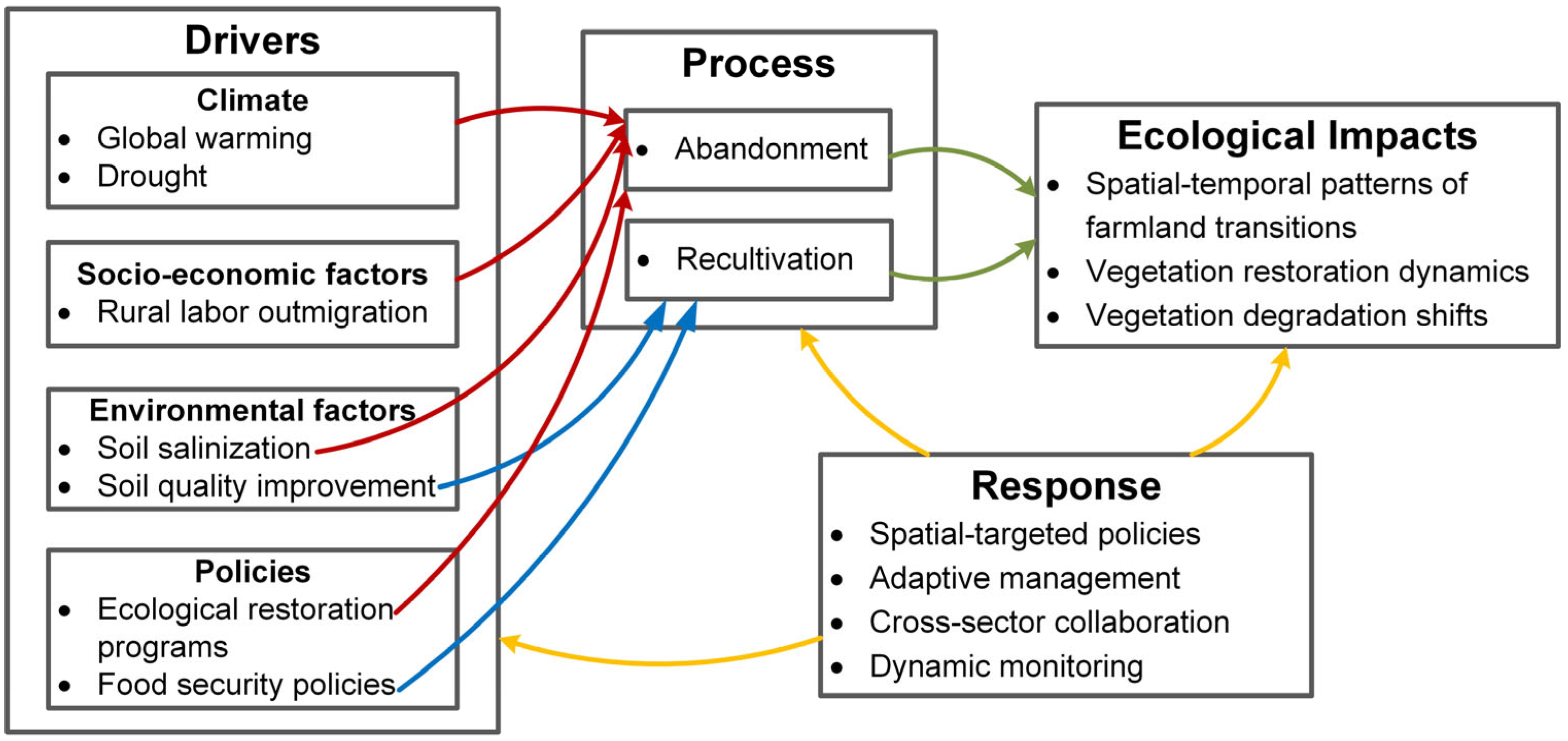
Figure 1. The conceptual framework. Red arrows denote drivers of abandonment; blue arrows signify drivers of recultivation; yellow arrows represent human–induced responses; and green arrows indicate the linkage from processes to ecological impacts.
Land 14 01745 g001
Figure 2. An overview of the Inner Mongolia section of the Yellow River Basin (IMYRB), derived from the 2021 annual China Land Cover Dataset (CLCD) [57].
Land 14 01745 g002
Figure 3. The overall view of sampling and validation sites. (a) The distribution of validation sites. (b1b3) The different temporal node in 2021. Focusing on the range of validation sites, both (c1,e1) are crops, while (c2,e2) are forest and bare soil, respectively. (d1,d2) and (f1,f2) are the interannual NDVI curves corresponding to (c1,c2) and (e1,e2).
Land 14 01745 g003
Figure 4. The flowchart of farmland abandonment and recultivation monitoring.
Land 14 01745 g004
Figure 5. FEI characteristics. (a) FEI values for different land cover types. (b) Temporal variation of FEI from 1999 to 2022. (c) The linear relationship between FEI values and the proportion of farmland.
Land 14 01745 g005
Figure 6. Empirical model for monitoring farmland abandonment and recultivation. (a) The abandonment ratio of farmland derived from Google Earth images. (b) The proportion of abandoned farmland as FAREI changes. (c) The proportions of recultivated farmland corresponding to various FAREIs.
Land 14 01745 g006
Figure 7. Sensitivity of farmland extraction accuracy to NDVI noise across FAREI thresholds.
Land 14 01745 g007
Figure 8. Interannual NDVI curves for various land surface types. Meanwhile, three temporally phenological nodes were also present.
Land 14 01745 g008
Figure 9. Spatiotemporal patterns and statistics of farmland abandonment and recultivation in the Inner Mongolia reach of the Yellow River Basin. (a,b) are the spatiotemporal distribution of abandonment and recultivation; (c,d) present the area statistics of abandonment and recultivation.
Land 14 01745 g009
Figure 10. Proportions of farmland abandonment and recultivation among topographic settings from 1999 to 2022.
Land 14 01745 g010
Figure 11. Vegetation restoration and degradation in the farmland abandonment area of the IMYRB from 1999 to 2022. The points shown in the figures do not represent actual pixel sizes. Instead, they were derived from raster-to-point conversion by ArcGIS, a procedure employed to improve visual clarity.
Land 14 01745 g011
Table 1. Details of data used in this paper.
Data
Collection
Temporal
Range
Spatial
Resolution
Spectral
Features
Product
Level
Access DateSources
MODIS2000 to 2022250 mNDVIMOD13Q1accessed on 23 March 2023https://ladsweb.modaps.eosdis.nasa.gov/
Landsat 51999 to 201230 mRed 1 and NIR 2 channelTM Reflectanceaccessed on 5 August 2023https://earthengine.google.com/
Landsat 82013 to 202230 mRed 3 and NIR 4 channelOLI Reflectanceaccessed on 22 August 2023https://earthengine.google.com/
SRTM30 mDEMSRTMGL1_003accessed on 13 May 2023https://earthengine.google.com/
CLCD1999 to 202130 mLand CoverVersion 1.0accessed on 6 July 2023https://doi.org/10.5281/zenodo.4417809
GLC30202030 mLand Coveraccessed on 9 July 2023http://www.webmap.cn/commres.do?method=globeIndex
Google Earth Image1999 to 2022Better than 15 mTrue coloraccessed on 10 September 2023https://earth.google.com/web/
Spectral range in wavelength for each channel, i.e., 1 0.63–0.69 µm, 2 0.76–0.90 µm, 3 0.63–0.68 µm, and 4 0.845–0.885 µm. All datasets were unified to UTM Zone 49N, WGS84.
Table 2. Coefficients of AIC.
CoefficientsValueCoefficientsValueCoefficientsValueCoefficientsValue
μ o 0.1672 ω 0.5479 t m 218 δ 0 −0.6059
μ α 0.5067 t s 128 δ α 0.6400
Table 3. Validation of farmland extraction accuracy.
Farmland
Extraction
Accuracy
(%)
YearPA (%)Margin of Error (PA, %)UA (%)Margin of Error (UA, %)OA (%)Margin of Error (OA, %)
199993.053.590.164.189.334.3
200295.192.993.193.592.673.6
200593.093.591.624.190.334.1
200892.393.590.054.189.843.7
201192.823.590.164.189.674.2
201493.223.589.674.289.274.2
201795.182.990.164.190.674.1
201993.333.590.064.189.334.3
202188.554.493.633.490.334.1
Note: Margin of error = half-width of a 95% Confidence interval (CI), n = 200.
Table 4. Accuracy comparison of different products.
This paperClassFarmlandNon-farmlandUser AccuracyMargin of Error (PA, %)Margin of Error (UA, %)Margin of Error (PA, %)
Farmland137894.48%3.93.24.3
Non-farmland134276.36%
Producer Accuracy91.33%84%Overall Accuracy 89.5%
GLC30ClassFarmlandNon-farmlandUser Accuracy4.84.55.1
Farmland1281788.28%
Non-farmland223360%
Producer Accuracy85.33%66%Overall Accuracy 80.5%
CLCDClassFarmlandNon-farmlandUser Accuracy5.24.95.5
Farmland1182781.38%
Non-farmland322341.82%
Producer Accuracy78.67%46%Overall Accuracy 70.5%
Note: Margin of error = half-width of a 95% Confidence interval (CI), n = 200.
Table 5. Validation of Farmland Abandonment and Recultivation Extraction Accuracy.
Farmland Abandonment and Recultivation Accuracy (%)YearPA (%)Margin of Error (PA, %)UA (%)Margin of Error (UA, %)OA (%)Margin of Error (OA, %)
1999–2002944.681.037.7866.8
2002–2005905.991.845.4915.6
2005–2008768.480.857.7798.1
2008–2011905.986.546.7886.4
2011–2014788.179.597.9798.1
2014–2017827.585.426.9847.2
2017–2019788.182.987.4817.7
2019–2022886.489.805.8896.2
Note: Margin of error = half-width of a 95% Confidence interval (CI), n = 100.
Disclaimer/Publisher’s Note: The statements, opinions and data contained in all publications are solely those of the individual author(s) and contributor(s) and not of MDPI and/or the editor(s). MDPI and/or the editor(s) disclaim responsibility for any injury to people or property resulting from any ideas, methods, instructions or products referred to in the content.