Abstract
Understanding food production (FP) supply–demand relationships is crucial for achieving Sustainable Development Goal 2 (SDG 2). Previous studies often assessed these relationships by overlaying supply and demand without considering food production flow (FPF). This study developed a framework from the perspectives of supply, demand, and flow to analyze the Agrifood System (AFS) of four major urban agglomerations in China: Beijing–Tianjin–Hebei, the Yangtze River Delta, the Pearl River Delta, and Chengdu–Chongqing. It applied the enhanced two-step floating catchment area model to simulate the magnitude and direction of four types of FPF—grains, vegetables, fruits, and meat—under three scenarios: intra-city flow, intra-provincial flow, and free flow. Results revealed mismatches in the FP supply–demand, and incorporating FPF improved these relationships. As flow restrictions eased, intra-city flows decreased, cross-regional flows expanded, and supply–demand imbalances were alleviated. Enhancing regional cooperation plays a key role in addressing the spatial mismatch between food supply and demand. These findings provide useful insights for addressing food supply–demand mismatches through more proper agricultural land allocation, better alignment of consumption patterns, and improvements in the flow system.
1. Introduction
In recent years, the achievement of SDG 2—to end all forms of hunger and malnutrition by 2030—has encountered unprecedented obstacles, driven by the compounded effects of extreme climate events, regional conflicts, and a deceleration in global economic growth. For example, the number of people suffering from hunger worldwide increased by 122 million in 2022 compared to pre-pandemic levels in 2019, with an estimated 9.2% of the global population undernourished, up from 7.9% in 2019 [1]. As the world’s largest developing country, China sustains nearly 20% of the global population with only 9% of the world’s arable land. In 2022, China produced 687 million tons of grain, of which 633 million tons were cereals, accounting for nearly 23% of the world’s total cereal output. By maintaining basic self-sufficiency in grain and absolute security in staple food, China has not only ensured domestic stability but also made significant contributions to global food security. However, with growing urbanization and regional disparities in production capacity and consumption demand, internal spatial mismatches in food supply and demand have become increasingly prominent. To further meet the growing demand for diverse food consumption and nutritional health, the Chinese government has proposed the “Big Food Version,” which aims to establish a diversified food supply system. Given the high population density in urban agglomerations, these regions are particularly vulnerable to food supply crises. Therefore, an in-depth analysis of food supply–demand relationships within Chinese urban agglomerations is not only essential for addressing the spatial mismatch between food supply and demand but also for providing critical support for the global achievement of SDG 2.
The Beijing–Tianjin–Hebei (BTH), Yangtze River Delta (YRD), Pearl River Delta (PRD), and Chengdu–Chongqing (CC) urban agglomerations have become the primary regions driving China’s urbanization [2]. However, rapid urban expansion and population concentration have severely challenged food supply security. In this context, applying a supply–demand–flow perspective enables a scientific understanding of how food transportation functions to address supply–demand mismatches. The specific objectives of this study are as follows: (1) Assess the FP static supply–demand relationships of four major food categories: grains, vegetables, fruits, and meat. (2) Simulate the flow direction and magnitude of FP under different administrative boundary constraint scenarios using a modified E2SFCA. (3) Reveal the FP dynamic supply–demand relationships from a supply–demand–flow perspective. The findings of this study will provide important scientific support for addressing the spatial mismatch between food supply and demand.
2. Literature Review
Food is one of the most essential provisioning services in ecosystem services [3,4], providing fundamental material resources for human survival. However, due to disparities in agricultural land endowments and socioeconomic development levels, a spatial mismatch exists between the supply and demand of FP. Existing studies predominantly analyzed the quantitative and spatial matching of FP based on local supply and demand, which were typically estimated using per capita consumption and total production data from statistical yearbooks [5,6,7,8,9,10] to identify and mitigate FP supply–demand imbalances [11].
FPF refers to the directional flow of food along transportation networks from Service Providing Areas (SPAs) to Service Benefiting Areas (SBAs) [12,13,14]. The SBAs maintain food supply–demand balances by integrating resources from both local and remote agricultural ecosystems. Unlike static supply–demand analyses that focus solely on food availability within administrative boundaries, the FPF framework highlights how surplus regions support deficit regions through spatial flows. By capturing the dynamic redistribution of food resources across space, it reveals how social systems derive sustenance from agricultural systems beyond their immediate locality, thus providing a more precise account of deficits, surpluses, and transfers from SPAs to SBAs [15].
Different FPF simulation methods focus on distinct dimensions, namely quantity, space, and process [16]. Quantity-based simulation methods generally define flow as the actual utilized FP, which can be directly measured by the amount of FP provided or indirectly inferred from the number of beneficiaries [17,18,19]. Space-focused simulation methods emphasize the direction and extent of FPF but do not consider the detailed flow process [20,21]. In contrast, process-based simulation methods offer a more comprehensive perspective by considering both the generation of FP and its quantity and spatial dynamics as it flows along specific pathways from SPAs to SBAs [11,22,23,24,25,26]. Since FP is a quantifiable material flow with clearly defined SPAs and SBAs, and follows specific transportation routes for directional flow, accessibility models based on transportation networks demonstrate strong applicability and scientific validity in simulating FPF. These spatial accessibility models primarily include the Gravity Model, the Breaking Point Model, and the Enhanced 2 Step Floating Catchment Area (E2SFCA) [27,28,29]. However, both the Gravity Model and the Breaking Point Model overlook the effective coverage of FP [30]. The E2SFCA, by incorporating distance thresholds, allows for a differentiated evaluation of FP supply capacity within the effective spatial range [30,31].
While recent research has attempted to address certain limitations in FP supply, demand, and flow [11,22,23,26], several key issues remain underexplored and warrant further attention. First, current assessments of food supply and demand remain limited in their consideration of food diversity and spatial heterogeneity. Many studies focus exclusively on grains, neglecting the complexity of diversified food systems [11,29]. Although some research has incorporated multiple food types [7,8,32], it often adopts simplistic aggregation methods based on weight or caloric content, overlooking the irreplaceability and spatial heterogeneity of different food types. This limitation has hindered the accurate representation of regional food production and consumption structures. Second, existing studies analyzing FP supply–demand dynamics have predominantly focused on local balance [15], failing to fully consider the role of FPF in mitigating supply–demand imbalances. This oversight may lead to misjudgments regarding FP supply–demand mismatches, as they are influenced not only by supply and demand but also by the spatial flows of FP, especially in regions with heavy reliance on interregional transport. Finally, current FPF simulations often disregard competition effects among SPAs and the surplus spillover [28,29]. When an SBA receives food from multiple SPAs, competition exists among these SPAs, meaning they collectively meet the SPAs’ demand rather than each independently supplying the full requirement. However, existing models fail to capture this competitive mechanism, leading to overestimation of demand. Furthermore, whether surplus food generated by competitive effects among SPAs can bridge demand gaps in other SBAs within a feasible transport range remains underexplored. Based on these gaps, this study seeks to address the following key question: from where do flows of various food categories originate, where do they ultimately reach, and to what extent do they alleviate supply–demand deficits in SBAs?
3. Materials and Methods
3.1. Study Area
China’s four national-level urban agglomerations—BTH, YRD, PRD, and CC—are located in the north, east, south, and west, respectively, and are designated as key growth engines under the national new-type urbanization strategy (Figure 1). These urban agglomerations, marked by strong economies, high population densities, and limited land resources, reflect a structural mismatch between population demand and land resource supply under specific spatiotemporal contexts, a typical manifestation of human–land conflict during rapid urbanization [33].
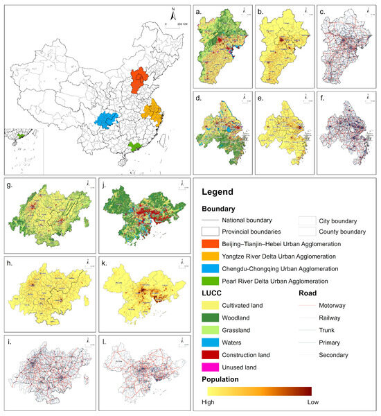
Figure 1.
Overview of the study area: (a–c) BTH; (d–f) YRD; (g–i) CC; (j–l) PRD.
Beijing–Tianjin–Hebei (BTH) comprises 3 provinces/municipalities (Beijing, Tianjin, and Hebei), covering 13 prefecture-level cities. While Beijing and Tianjin are densely populated and concentrate major socioeconomic activities, Hebei exhibits significant agricultural strengths. BTH has a population of approximately 110 million (7.8% of the national total) and 17.06 million hectares of agricultural land (2.5% of the national total). Its GDP reached RMB 10.03 trillion in 2022 (Table 1).

Table 1.
Socioeconomic status of the selected urban agglomerations.
The Yangtze River Delta (YRD) includes 3 provinces/municipalities (Shanghai, Jiangsu, and Zhejiang), covering 41 cities. It is a globally competitive urban agglomeration. It houses 16.8% of China’s population but has only 2.5% of national agricultural land (17.06 million ha), indicating a severe spatial mismatch between food demand and supply capacity. YRD leads the country in economic performance, with a GDP of RMB 24.25 trillion, accounting for nearly one-fifth of the national total.
The Pearl River Delta (PRD) consists of 9 cities in Guangdong Province. It has a population of about 78 million (5.5% of the national total), but only 4.10 million hectares of agricultural land (0.6% of the national total), rendering its human-land conflict particularly acute. Despite its limited land base, PRD’s GDP stands at RMB 10.47 trillion, underscoring its high economic density and resource pressure.
Chengdu–Chongqing (CC) includes 2 municipalities (Chengdu and Chongqing), with 16 prefecture-level cities. It accounts for 7.3% of the national population and 17.75 million hectares of agricultural land (2.6% of the national total), making it the most agriculturally abundant among the four urban agglomerations. Its GDP reached RMB 7.97 trillion.
3.2. Methodological Framework
To systematically analyze the spatial dynamics of Agrifood System (AFS), we established a supply–demand–flow framework that captures the interactions among food production, transportation, and consumption. As shown in Figure 2, this framework conceptualizes food-producing areas, food-consuming areas, and the directional flows of food between them. The E2SFCA was then employed to quantify the magnitude and direction of these flows, incorporating spatial impedance and supply–demand ratios.
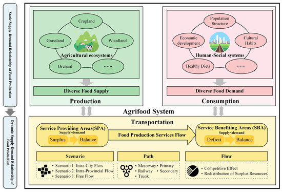
Figure 2.
Methodological framework.
AFS encompasses multiple stages, including food production, transportation, and consumption [34,35]. Agricultural ecosystems provide material support to social systems through the provision of diverse food products. Meanwhile, social systems generate complex food demands due to a multitude of factors, such as population structure, economic development, and cultural diets [36]. However, the spatial distribution of food production and consumption does not always overlap [11,15,28], resulting in a spatial mismatch between local supply and demand in the absence of food flows. When a region produces a food surplus after meeting its own consumption needs [25,37], it can serve as an SPA by exporting the excess food via transport networks. Conversely, regions with a net demand exceeding local supply are identified as SBAs [11,23,38]. In our research, each county is treated as an integrated unit and identified as either an SPA or an SBA for a given food type, based on its static supply–demand balance. This provides the basis for analyzing the FPF among counties within each urban agglomeration. Given the influence of cross-regional spatial flows of FPF [39], incorporating food supply, demand, and flow provides a more comprehensive representation of the spatial distribution and resource allocation of FP.
3.3. Simulation of Food Production Flows
This study employed E2SFCA to simulate the direction and magnitude of FPF for four types of food: grain, vegetables, fruits, and meat. The E2SFCA improves the traditional 2SFCA by incorporating a distance–decay function to better capture the attenuation of food supply capacity over space. This method enables a nuanced spatial analysis of how food produced in surrounding areas meets the demand of urban agglomerations, considering both supply intensity and spatial impedance. It is especially suited to quantify the food supply–demand balance under various flow patterns. The required data, including agricultural production, population distribution, land use, and road network information, as well as the construction of the network dataset, are detailed in Appendix A.
Step 1: SPAs and SBAs are determined based on the static supply–demand relationships, calculated using food production and local consumption data (see Appendix B). A search domain is established for a given food supply node , defined by the maximum reachable distance within a specified time threshold along the transportation network. Aggregate all the demand quantities within the search domain , assign weights based on the distance decay rule using a Gaussian function, and sum the weighted demand quantities to calculate the supply–demand ratio :
where denotes the deficitat a specific food demand node. represents the surplus at the supply node. represents the travel time between the supply node and the demand node, requiring the demand node to lie within the search domain. Considering factors such as shelf life and transportation losses for different types of foods, the thresholds are set to 48 h for grain, 12 h for vegetables, 24 h for fruits, and 12 h for meat. While no universal standards exist for these parameters, their settings reflect practical time constraints under normal logistics conditions. is the Gaussian decay function, given by the following equation:
Step 2: For any demand node of a certain food type, a search domain is established with its corresponding time threshold as the radius. All supply nodes within this domain are then identified, and their supply–demand ratios are aggregated using a Gaussian decay function to obtain the initial supply–demand ratio for that demand node:
Step 3: Considering that competition among supply nodes may result in the same demand being satisfied multiple times, for demand nodes with an initial supply–demand ratio > 1, the demand is proportionally adjusted based on and then redistributed to the respective supply nodes. The adjusted flow (, representing the flow from the supply node to the demand node, is calculated as the product of the adjusted demand and the supply–demand ratio .
Residual resources may remain at supply nodes due to the adjustments made to the flows between supply and demand nodes ( > 1). In such cases, if unmet demand still exists within the movement range, the above steps must be iteratively repeated to further allocate the surplus resources from the supply nodes to the demand nodes within the range, until the residual resources are maximally utilized or the demand gap is completely filled.
To analyze the impact of administrative boundary constraints (i.e., the institutional constraints on food circulation imposed by city- and province-level jurisdictions) on FPF, this study examined the FPF of four food types—grain, vegetables, fruits, and meat—under three scenarios: (1) Scenario 1: intra-city flow; (2) Scenario 2: intra-provincial flow; (3) Scenario 3: free flow. These scenarios represent progressively relaxed spatial constraints, simulating real-world food flow patterns under varying levels of administrative coordination. It is important to note that FPF was first restricted by this distance threshold to ensure realistic transport feasibility, meaning that circulation was only allowed if both counties were located within the specific transport distance in all scenarios. Additionally, crossing administrative boundaries may incur additional time costs, such as those resulting from passage inspections or administrative approvals. Therefore, buffer zones were established along both provincial and municipal boundaries and treated as polygon barriers, thereby simulating the resistance to cross-boundary flow.
3.4. Evaluation of Dynamic Supply–Demand Relationships in Food Production
By integrating the static supply–demand balance of FP with simulated flow patterns, this study evaluated the dynamic supply–demand relationships—specifically, the reconfigured spatial distribution of FP supply–demand relationships after accounting for FPF—under the three scenarios. The total from each supply node and the total to each demand node were aggregated to compute the final dynamic supply–demand relationships.
3.5. Analyzing the Agrifood System
This study employed three indicators—network density, the Gini coefficient, and average transport time—to assess the effectiveness of addressing the spatial mismatch between food supply and demand under various scenarios.
Network density is used as an indicator of the connectivity of the FPF network [40,41], which is directly related to the system’s stability under disturbances. A higher density indicates more alternative pathways between SPAs and SBAs, thereby enhancing buffering capacity during disruptions. Since this study assumes that food must first satisfy local demand, the maximum theoretical number of edges in the flow network is the product of the number of supply nodes and the number of demand nodes:
where represents network density, is the number of edges in the FPF network, is the number of supply nodes, and is the number of demand nodes.
By calculating the Gini coefficient of the FP dynamic supply–demand ratio across all counties within each urban agglomeration [42,43], this study quantifies the spatial equity of food allocation. A lower Gini coefficient indicates a more balanced distribution of food relative to demand among counties, suggesting a more equitable food access pattern.
where and represent the FP dynamic supply–demand ratio for supply and demand nodes, respectively. is the Gini coefficient, ranging from 0 to 1, with lower values indicating a higher level of equity within the AFS.
The efficiency of the FPF network is assessed by the average food transport time. A shorter average transport time indicates higher FP flow efficiency, reducing food loss and transportation costs.
4. Results
4.1. Food Production Flows and Dynamic Supply–Demand Relationships
The magnitude and direction of the FPF for the four food types at the county scale were analyzed under three flow scenarios: intra-city, intra-province, and free flow. Furthermore, the dynamic supply–demand relationships of the FPF, incorporating supply, demand, and flow factors, were examined to understand how the flow influences the relationships.
4.1.1. Scenario 1: Intra-City Flow Only
Regarding grain, the total flow in BTH was 2.63 × 10⁶ tons, distributed across all 14 cities except Hengshui (Figure 3). Compared to static supply–demand relationships (Appendix C), the FPF significantly alleviated the grain supply–demand imbalance in BTH, but 21.10% of the population remained in grain-deficit areas. In YRD, 1.78 × 10⁶ tons of grain participated in the flow, primarily concentrated in the eastern and northern regions. However, 62.39% of the population still resided in grain-deficit areas. The grain flow within cities in the PRD amounted to 2.96 × 10⁵ tons. The FPF led to a 5.67% reduction in the population living in grain-deficit areas in the PRD. The grain flow in CC reached 1.92 × 10⁶ tons, and currently, only the counties in central CC still exhibit a grain deficit, where 15.17% of the region’s population resides.
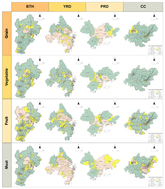
Figure 3.
FP flow and dynamic supply–demand relationships in different urban agglomerations under Scenario 1. Note: Line thickness indicates FPF magnitude (see legend).
In terms of vegetables, the flow in BTH was 3.35 × 10⁶ tons, with 22.93% of the population transitioning from vegetable-deficit to vegetable-surplus areas due to the FPF. Only the counties in central Beijing still exhibited a vegetable deficit. The total flow in YRD was 3.27 × 10⁶ tons, enabling 20.24% of the population to overcome the vegetable supply–demand imbalance. However, some counties in Wuxi, Shanghai, and Zhoushan still faced vegetable shortages. The total vegetable flow in PRD was 1.14 × 10⁶ tons, but 54.25% of the population in the central and southern regions remained in vegetable-deficit areas. In CC, 1.41 × 10⁶ tons of vegetables were involved in the flow, and all the previously deficit counties achieved supply–demand balances.
Regarding fruits, the total flow in BTH was 2.53 × 10⁶ tons, significantly alleviating the fruit supply–demand imbalance, with a 36.24% decrease in the population residing in fruit-deficit areas. The total flow in YRD was 1.36 × 10⁶ tons. Nevertheless, 37.06% of the population still lived in deficit areas, primarily in Shanghai and Jiangsu. In PRD, 7.29 × 10⁵ tons of fruits participated in the flow, which alleviated the fruit deficit for 24.51% of the population. The total fruit flow in CC was 9.74 × 10⁵ tons. Similar to vegetables, intra-city flow met the supply–demand gap in all deficit areas.
The meat flow in BTH was 6.47 × 10⁵ tons, addressing the supply–demand imbalance for 19.42% of the population, but severe imbalances in meat supply and demand persisted in Beijing, Tianjin, and Langfang. The total flow in YRD was 4.39 × 10⁵ tons, resolving the supply–demand deficit for only 6.51% of the population, while 76.77% still lived in meat-deficit areas. The situation was even worse in PRD, where 2.33 × 10⁵ tons of meat flow alleviated the supply–demand deficit for just 3.21% of the population, leaving 83.17% of the population’s meat demand still unmet. Similarly, the meat flow in CC was 3.33 × 10⁵ tons. However, 33.35% of the population—primarily in central Chengdu and southern Chongqing—remained in meat-deficit areas.
4.1.2. Scenario 2: Intra-Province Flow Only
Regarding grain, compared to Scenario 1, in the intra-province flow scenario, the grain deficit situation in BTH remained unchanged, while the deficit areas in YRD and CC shrank, but the deficit issue in PRD worsened (Figure 4). Specifically, the total grain flow in BTH was 2.63 × 10⁶ tons, with 62.45% of the flow being inter-city. The grain flow and dynamic supply–demand relationships were the same in Scenario 1 and Scenario 2. The total flow in YRD was 4.57 × 10⁶ tons, with 95.52% of the flow being inter-city. Compared to Scenario 1, the resident population in deficit areas decreased by 30.99 million people, but 44.35% of the population still lived in deficit areas, primarily in Shanghai and Zhejiang. In CC, 2.15 × 10⁶ tons of grain participated in the flow, with 62.45% being inter-city flow. In Scenario 2, the entire CC region solved the grain supply–demand deficit problem. PRD, being the only urban agglomeration located entirely in a single province, was not affected by provincial boundaries. However, the removal of flow restrictions did not fully resolve the grain deficit in any county in PRD. While external replenishment through FPF partially addressed the local grain demand gap, compared to Scenario 1, the extent of deficit areas in PRD expanded, as in the static supply–demand relationships (Appendix C).
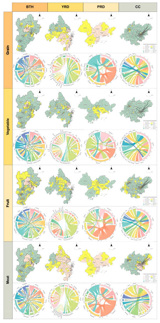
Figure 4.
FP flow and dynamic supply–demand relationships in different urban agglomerations under Scenario 2. Note: Line thickness indicates FPF magnitude (see legend).
Regarding vegetables, compared to Scenario 1, the supply–demand relationships in BTH remained unchanged, while the deficit issue in YRD improved, PRD eliminated deficits in all counties, and CC had already achieved vegetable supply–demand balances in Scenario 1. Specifically, in BTH, the total flow and dynamic supply–demand relationships in Scenario 1 and Scenario 2 were identical. The difference was that in Scenario 2, 41.33% of the flow was inter-city. In YRD, 3.43 × 10⁶ tons of vegetables were involved in the flow, with 72.40% being inter-city. Nevertheless, 12.95% of the population still lived in deficit areas. The total flow in PRD was 3.54 × 10⁶ tons, with 93.47% of the flow being inter-city, leading to the complete elimination of vegetable deficits across the region.
Regarding fruits, the supply–demand relationship between BTH and YRD improved, PRD eliminated fruit deficit areas across the region, and CC had already achieved self-sufficiency in Scenario 1. Specifically, the total flow in BTH was 2.60 × 10⁶ tons, with 77.49% being inter-city. Compared to Scenario 1, Scenario 2 only resolved the fruit deficit in Zhangjiakou. The expanded flow range did not significantly improve the supply–demand relationships. The fruit flow in YRD was 2.35 × 10⁶ tons, with 95.17% being inter-city. Compared to Scenario 1, the fruit demand gap was reduced by 38.00 million people. However, some counties in Shanghai and Zhoushan still faced deficits, where 14.95% of the population lived. In PRD, 2.30 × 10⁶ tons of fruit participated in the flow, with 94.98% being inter-city. Compared to Scenario 1, the fruit demand gap for 43.86 million people was filled, and PRD achieved fruit self-sufficiency across the entire region.
The meat situation was generally similar to that of grain. Specifically, in BTH, the flow and dynamic supply–demand relationships in Scenario 1 and Scenario 2 were identical, with 62.17% of the meat flowing inter-city. The total flow in YRD was 1.22 × 10⁶ tons, with 93.20% of the flow being inter-city. Compared to Scenario 1, the meat demand gap for only 4.6819 million people was resolved. However, 74.05% of the population’s meat demand in YRD remained unmet. The meat flow in CC was 8.12 × 10⁵ tons, with 84.21% of the flow occurring between cities. As a result, 21.31% of the population in previously meat-deficit counties achieved self-sufficiency through redistribution via the FPF network. However, most counties in Chongqing still faced deficit areas. In PRD, 7.10 × 10⁵ tons of meat were involved in the flow, with 96.93% of the flow being inter-city. Although both the flow and flow range increased compared to Scenario 1, 86.38% of the population in PRD still lived in meat supply–demand deficit areas. The meat FPF mitigated supply–demand imbalances in all previously deficit areas, but none of these areas transitioned into surplus or fully balanced status compared to the static supply–demand baseline (Appendix C).
4.1.3. Scenario 3: Free Flow
Under Scenario 3, various food types were allowed to flow freely across cities and provinces, as long as the transportation time between supply and demand nodes remained within the defined travel time thresholds (Figure 5). Since PRD was entirely located within Guangdong Province, its Scenario 2 and Scenario 3 outcomes were identical; thus, it was not discussed below. Overall, under Scenario 3, all regions achieved a balance in the supply and demand of all food types, except that YRD still exhibited a meat supply–demand imbalance.
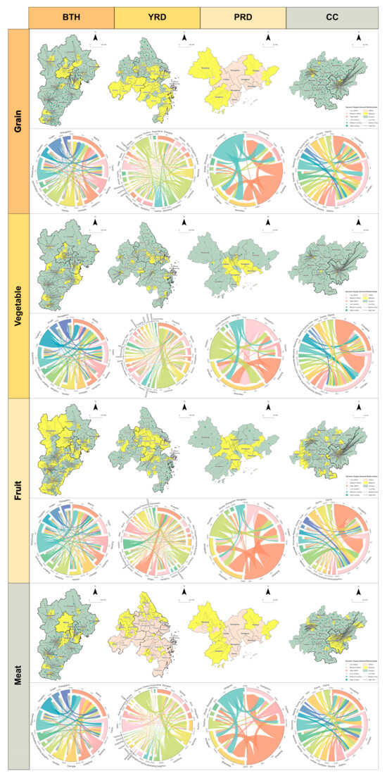
Figure 5.
FP flow and dynamic supply–demand relationships in different urban agglomerations under Scenario 3. Note: Line thickness indicates FPF magnitude (see legend).
In terms of grains, BTH eliminated its deficit areas, YRD essentially achieved grain self-sufficiency, and CC had already attained the overall supply–demand balance in Scenario 2. Specifically, the total grain flow in BTH was 4.29 × 10⁶ tons, of which 55.63% was inter-provincial flow. Compared to Scenario 2, the population in deficit areas decreased by 22.55 million, and the grain demand gap was fully met in all counties. In YRD, the total grain flow reached 9.81 × 10⁶ tons, with 76.59% being inter-provincial. However, because Zhoushan is located on an island and grain could not be transported by road or rail, 1.27% of the population remained in grain supply–demand deficit areas. CC had already attained food supply–demand equilibrium in Scenario 2. The distinction in Scenario 3, however, lies in the fact that 39.49% of the food was transferred across provincial boundaries.
The dynamic supply–demand relationships for vegetables and grains were similar. In BTH, the total vegetable flow was 3.76 × 10⁶ tons, with 58.68% constituting inter-provincial flow. Under this scenario, vegetable demand was met in all counties across the region. In YRD, 4.23 × 10⁶ tons of vegetables were involved in the flow, with 54.84% being inter-provincial. Considering both local supply and inflows from other counties within the YRD, vegetable deficits were resolved across most of the region, with the exception of Zhoushan. In CC, the vegetable deficit had already been resolved in Scenario 2. And under Scenario 3, 43.35% of the flow was inter-provincial.
Similarly, in terms of fruits, BTH had a total fruit flow of 4.11 × 10⁶ tons, with 44.21% of the flow consisting of inter-provincial FPF. The further expansion of the flow range completely resolved the regional deficit issues. Compared to Scenario 2, the population in deficit areas decreased by 33.9283 million, accounting for 31.75% of BTH’s total population. In YRD, the total fruit flow was 3.49 × 10⁶ tons, with the inter-provincial share reaching as high as 75.52%. Except for Zhoushan, YRD achieved fruit self-sufficiency across the region. In Scenario 2, CC had already fully met the fruit demand of all counties; however, under Scenario 3, 41.67% of the flow was inter-provincial.
In terms of meat, BTH and CC achieved meat self-sufficiency, whereas the dynamic supply–demand relationships in YRD deteriorated relative to Scenario 2. Specifically, BTH’s total meat flow was 1.33 × 10⁶ tons, with 64.32% representing the inter-provincial flow. Compared to Scenario 2, the deficit population in BTH decreased by 34.21 million people, thereby achieving meat self-sufficiency across the region. In CC, the total meat flow was 1.19 × 10⁶ tons, with inter-provincial flow accounting for 39.22%. The removal of inter-provincial flow restrictions eliminated meat supply–demand deficit areas throughout CC. In YRD, 1.33 × 10⁶ tons of meat flowed, with 54.67% being inter-provincial. However, compared to the static supply–demand relationships (Appendix C), the FPF did not substantially resolve the meat supply–demand deficit in any county, with 83.28% of the population still having unmet meat demand.
4.2. Analysing Agrifood Systems Across Different Scenarios
With the gradual lifting of flow restrictions, the AFS in the various urban agglomerations exhibited both common characteristics and regional differences. Overall, the FPF network showed stronger connectivity under constrained conditions, as indicated by increased network density; meanwhile, the spatial distribution of food became more balanced across regions, as reflected by changes in the Gini coefficient. However, average transportation time increased (Figure 6). Firstly, in terms of network density, the FPF network in YRD was the least resilient, whereas the levels in BTH, PRD, and CC were relatively similar. In terms of the magnitude of change, after the removal of municipal-level administrative boundary restrictions, the network density in BTH, PRD, and CC improved significantly, whereas the improvement in YRD depended more on the lifting of provincial-level administrative boundary restrictions. Secondly, regarding the Gini coefficient, PRD had the highest Gini coefficient, unequal food distribution, while CC exhibited the most equitable distribution, with BTH and YRD falling in between. From Scenario 1 to Scenario 2, the Gini coefficient decreased significantly in YRD, PRD, and CC, whereas the reduction in BTH mainly resulted from the removal of provincial-level administrative boundary restrictions. Finally, for average transportation time, YRD recorded the longest average transportation distance and the lowest flow efficiency, followed by BTH, while CC and PRD experienced shorter average transportation distances and relatively higher flow efficiency. After the removal of municipal-level administrative boundary restrictions, the average transportation time in BTH, PRD, and CC increased significantly, while YRD’s transportation time increased substantially, primarily due to the lifting of provincial-level administrative boundary restrictions.
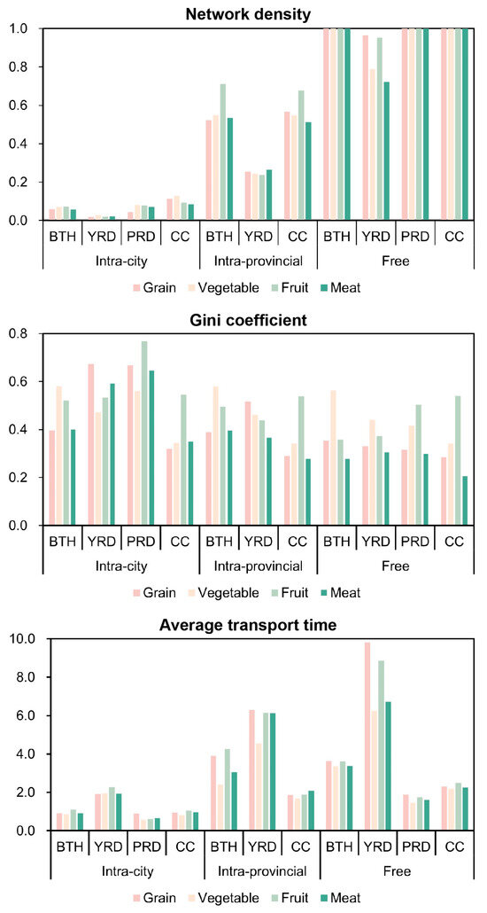
Figure 6.
Network Density, Gini Coefficient, and Average Transport Time of AFS in Four Urban Agglomerations under Different Scenarios.
5. Discussion
5.1. Integrating Supply, Demand, and Flows to Reveal Food Production Deficit
Understanding the diversified FP supply–demand relationships—shaped by regional disparities in production capacity, food-specific consumption patterns, and flow dynamics—is essential for fostering a sustainable AFS. However, existing studies have predominantly focused on grains [15,22,28,29,44] or have studied multiple food types as a whole [9,45,46], thereby overlooking the irreplaceability and spatial heterogeneity of different food categories. On the one hand, each food category provides essential nutrients indispensable for promoting a balanced diet and improving nutritional outcomes. On the other hand, our study revealed that the spatial distribution patterns of FP supply–demand relationships exhibited marked heterogeneity across different food categories.
AFS involves multiple stages of food production, transportation, and consumption. Understanding the challenges and dynamics at each stage—from optimizing agricultural land allocation and adjusting dietary demand patterns to enhancing food flow systems—enables policymakers to design integrated strategies that promote sustainable and resilient food systems. Notably, traditional static supply–demand analyses merely reflect local supply–demand matches. In reality, however, SBAs often rely on both local and external supplementation [11]. Unfortunately, due to the difficulty of obtaining historical food trade data [32], accurately evaluating FPF remains a challenge. Existing studies primarily employed the E2SFCA to assess grain ecosystem service flows [28,29]. However, this model overlooked the competitive effects among SPAs and the allocation of spillover FPF [47]. To address these issues, our study modified the E2SFCA. Specifically, our study reduced the external supplementation for SBAs with an initial supply–demand ratio and redistributed the resultant overflow food to simulate FPF more accurately and realistically. Furthermore, the study simulated FPF under different administrative boundary constraint scenarios, exploring how interregional collaboration could facilitate resource sharing to improve local food supply–demand imbalances. The results indicated that as administrative boundary restrictions were relaxed, the flow range gradually expanded, intra-urban flow diminished, and cross-regional flow increased. Administrative boundaries constituted, to some extent, institutional barriers to interregional resource flows, confining food allocation to relatively smaller areas. When these restrictions were progressively lifted, SBAs that once relied solely on local food supplies could bridge their supply–demand gaps through external supplementation, thereby preventing resource depletion in certain critical SPAs due to over-allocation.
Previous studies have typically analyzed food supply–demand deficits based on the FP static supply–demand relationships [9,15,45,48], yet they have overlooked the role of FPF in ameliorating supply–demand imbalances. In this study, in addition to assessing the static supply–demand relationships, flow considerations were incorporated to explore the FP dynamic supply–demand relationships under different scenarios. The results indicated significant differences between static and dynamic supply–demand relationships across various scenarios [11]. A horizontal comparison among four urban agglomerations revealed that core cities in each cluster generally exhibited FP static supply–demand deficits, as observed in Beijing, Shanghai, Guangzhou, and Shenzhen. However, as food flow restrictions were gradually relaxed, for urban agglomerations with adequate food sources, the number of people in deficit areas was gradually reduced, and the mismatch between food supply and demand was completely resolved. In contrast, four urban agglomerations with scarce food resources, although expanding the flow range did not entirely eliminate regional deficits, FPF still significantly alleviated the supply–demand contradictions in these deficit areas through the reallocation of resources.
5.2. Understanding Efficiency in Agrifood Systems Across Scenarios
This study compared the commonalities, differences, and variations in network density, the Gini coefficient, and average transportation time of AFS under different scenarios. Overall, as flow restrictions were gradually lifted, AFS across urban agglomerations generally exhibited increased network density and more balanced food distribution but longer transportation times. First, regarding network density, the expansion of flow increased the availability between SPAs and SBAs, enhancing the complexity and cohesion of the FPF network, and thereby improving overall network connectivity [22]. Consequently, when the system was subject to external disturbances, SBA could still obtain external supplies through alternative pathways even if certain SPAs or flow routes failed, demonstrating strong resilience. Regarding the Gini coefficient, the removal of flow restrictions facilitated the redistribution of food supplies over a broader spatial extent, leading to a general decline in the Gini coefficient of the supply–demand ratio. This indicated a gradual balancing of FP supply and demand within the system. However, in terms of average transportation time, the relaxation of flow constraint inevitably expanded the spatial scope of FPF, resulting in longer average transportation times. This change contributed to increased food loss, higher transportation costs, and greater carbon emissions [15,49,50,51], thereby reducing the efficiency of food transportation. In the context of China’s “Dual Carbon” goals—peaking carbon emissions before 2030 and achieving carbon neutrality by 2060—the increased emissions from long-distance food transportation raise important concerns. Therefore, improving the alignment between food supply and demand through coordinated planning and interregional cooperation is essential to reduce unnecessary transport distances while ensuring stable and equitable food access.
On the other hand, significant differences in these three indicators existed among the various urban agglomerations. The YRD exhibited the lowest network density and longest transport times among the four urban agglomerations. From the supply side, agricultural land resource endowments in the YRD varied considerably, with the main SPAs distributed along the northern and western margins. From the demand side, the population in the YRD was unevenly distributed; core cities concentrated large populations that generated substantial food demand, resulting in a high dependence on interregional food supply. In Scenario 1 and Scenario 2, the FPF network showed poor connectivity due to the constraints imposed by administrative boundaries. In Scenario 3, the uneven spatial distribution of SPAs and SBAs for various foods led to over 50% interprovincial FPF—a proportion that far exceeded that in other urban agglomerations. This resulted in the longest average food transportation times and the lowest efficiency in the YRD. Regarding the Gini coefficient, the PRD performed the worst, with its human-land conflicts being particularly pronounced among the four urban agglomerations. As the urban agglomeration with the highest urbanization rate in China, the concentration of population and the upgrading of dietary structures have driven increasingly diversified food demand. Meanwhile, the continuous expansion of construction land has encroached upon agricultural space, and the spatial distribution of agricultural land remains uneven. This has made it difficult for core cities such as Guangzhou and Shenzhen to achieve food self-sufficiency, forcing them to rely heavily on interregional FPF. Furthermore, the PRD faced severe supply–demand imbalances under all scenarios due to the relative scarcity of overall agricultural resources.
Finally, by comparing the magnitude of changes in the three indicators across different scenarios, it was evident that in most urban agglomerations, network density increased and the Gini coefficient decreased significantly following the removal of municipal administrative boundary restrictions. This stemmed from the relatively balanced allocation of resources among provincial administrative units within urban agglomerations, which enabled most provinces to achieve an internal equilibrium between food supply and demand. However, due to the expansion of the flow range and the constraints imposed by provincial administrative boundaries, some flow paths may become more circuitous, leading to a substantial increase in transportation time. Notably, after the removal of provincial administrative boundary restrictions, certain urban agglomerations exhibited significant changes in their indicators. There were great differences in resource endowments among provinces in YRD. As the main SBA, Shanghai and Zhejiang depended on the food supply of Jiangsu and Anhui. The removal of provincial border restrictions promoted inter-provincial food transportation, thus greatly enhancing network density. In terms of the Gini coefficient, the elimination of provincial boundary restrictions resulted in a marked reduction in the food distribution Gini coefficient in BTH. This outcome was attributable to the high population density and elevated urbanization levels in Beijing and Tianjin, which created a considerable gap in food demand. The lifting of provincial administrative boundary restrictions enabled Hebei’s food surplus to be allocated more efficiently to Beijing and Tianjin, thereby significantly balancing food distribution. For average transportation time, the average food transportation time in CC increased dramatically following the removal of provincial administrative division restrictions. Although the interprovincial FPF in CC had, to some extent, improved network density and reduced imbalance in food distribution, it only addressed the meat supply–demand imbalance in Chongqing. This suggests that for urban agglomerations with abundant food supplies, an expanded transportation range may not necessarily exert a positive impact on the overall performance of AFS.
5.3. Addressing the Spatial Mismatch Between Food Supply and Demand from the Perspective of Supply–Demand Flows
To improve the imbalances between food supply and demand, this study suggests that attention should be given to three specific areas: optimizing the allocation of agricultural land resources, adjusting demand patterns, and improving the flow system. These measures aim to strengthen the system’s ability to mitigate risks and accommodate diverse food needs. (1) Supply-Side Perspective: Agricultural land resource management should be systematically coordinated across three dimensions: quantity, quality, and ecology. In terms of quantity, it is essential to strictly protect high-quality agricultural land and restrict the encroachment of construction land into agricultural areas. Simultaneously, considering the diversification of food demand, spatial patterns, and functional zoning of agricultural land should be coordinated to improve the allocation of cropland, forestland, and grassland. Regarding quality, agricultural productivity can be improved through measures such as intensive and efficient land use, the development of high-standard farmland, and land reclamation and consolidation [52,53]. In terms of ecology, the ecological protection and restoration of cropland should be strengthened, and the negative impact of agricultural production on the environment should be mitigated to build a sustainable agricultural ecosystem. Meanwhile, considering the spatial limitations of land use in densely populated urban agglomerations, innovative agricultural models such as urban agriculture [54,55] and vertical farming [56] can provide viable alternatives for enhancing local food supply. These models utilize underused urban spaces (e.g., rooftops, abandoned buildings, and vertical structures) to grow food efficiently within cities, reducing transportation distances and improving local supply capacity. (2) Demand-Side Perspective: Given the Limited agricultural land resources in urban agglomerations that struggle to meet the growing demand for food, promoting healthy dietary habits is crucial to alleviating food supply–demand imbalances. Especially in YRD and PRD, even in the free-flow scenario, 83.28% and 86.38% of the population are still distributed in meat supply–demand deficit areas. However, according to the Chinese Dietary Guidelines [57], the recommended daily intake of livestock and poultry meat for adults is 40–75 g, whereas the per capita meat consumption in the YRD and PRD significantly exceeds this standard. This indicates an urgent need to shift dietary preferences toward more plant-based and diversified food sources. In line with China’s ‘Big Food Version ‘ strategy [58,59], efforts to address food supply–demand mismatches should not rely solely on cultivated land resources but should instead draw on the entirety of national land resources, promoting the diversified and multi-path food sources to meet the growingly diverse demands of food consumption. (3) Flow-Side Perspective: Improving food flow networks to address supply–demand mismatches should be guided by three principles: strengthening regional connectivity, balancing food distribution, and reducing transport time. To strengthen regional connectivity, it is necessary to enhance the agricultural product reserve system and the cold chain processing and distribution system to ensure timely responses to emergencies and maintain stable FPF. To balance food distribution, reducing administrative constraints—defined here as limitations on inter-jurisdictional food flows between cities and provinces—may help facilitate a more coordinated and efficient regional food flow system, thereby mitigating spatial mismatches in food supply and demand. However, based on our simulations under different administrative boundary scenarios, it becomes clear that differentiated coordination mechanisms are necessary across urban agglomerations. For BTH, where network connectivity and transport time are particularly sensitive to interprovincial constraints, priority should be given to enhancing cross-provincial institutional collaboration. In contrast, in YRD, PRD, and CC, most food flows can be effectively coordinated within provincial boundaries, so improving inter-municipal integration may yield more immediate and practical benefits. That said, special attention must be paid to municipalities like Shanghai and Chongqing. As centrally administered cities that do not belong to any province, their food inflows inevitably require cross-provincial transportation. Given their high urbanization levels and limited agricultural land, failure to strengthen interprovincial coordination could leave these key cities structurally isolated within otherwise internally coordinated regional food systems. To reduce transport time, a relatively balanced spatial arrangement of SPAs and SBAs should be pursued to ensure that SPAs are appropriately distributed around SBAs, minimizing reliance on long-distance transport and improving supply–demand alignment. These measures contribute to the long-term sustainability of the AFS.
6. Conclusions
Based on the AFS framework, this study explored the spatial flow characteristics and dynamic supply–demand relationships of FP for different food types in China’s four major urban agglomerations under various scenarios. The study focused on addressing the question: To what extent did the FPF, under different administrative boundary restrictions, improve the supply–demand relationships of FP? The results indicated that, at the county scale, the spatial distribution of the static supply–demand relationships of FP in BTH, YRD, PRD, and CC exhibited significant differences, with a large population residing in areas of imbalanced supply and demand. The FPF effectively alleviated these static imbalances. As administrative boundary restrictions were gradually relaxed, the flow range expanded, the scale of cross-boundary flow increased, and intra-city flow decreased. Urban agglomerations rich in food resources were able to address supply–demand mismatches through flow, whereas resource-scarce urban agglomerations primarily relied on flow to redistribute resources; although deficits were not entirely eliminated, the flow significantly alleviated supply–demand conflicts. Overall, these urban agglomerations exhibited a general trend of increased network connectivity and more balanced food distribution, but longer average transport times. Based on a supply, demand, and flow perspective, policy recommendations were proposed to address food supply–demand mismatches.
Nonetheless, this study has several limitations that should be acknowledged. First, the simulation assumes that surplus food can be fully reallocated within the transport time thresholds, without considering real-world factors such as market dynamics and transaction costs, which may affect the actual flow of food. Second, the model’s parameterization may not fully reflect the complexity of real-world conditions influencing food supply–demand flows. Future research should aim to integrate these factors into the modeling framework. Moreover, as more detailed and reliable food flow datasets become available, future studies should prioritize validating simulated patterns against real-world data to enhance model accuracy and provide stronger support for strategies to address food supply–demand mismatches.
Author Contributions
Conceptualization, C.Y. and R.M.; methodology, R.M.; data curation, R.M.; writing—original draft preparation, R.M.; writing—review and editing, C.Y.; visualization, R.M.; supervision, C.Y. All authors have read and agreed to the published version of the manuscript.
Funding
This research was funded by the Ministry of Education of Humanities and Social Science project, grant number 21YJA790006 and Fundamental Research Funds for the Central Universities, grant number 2025ZDJC003.
Data Availability Statement
Dataset is available on request from the authors.
Conflicts of Interest
The authors declare no conflicts of interest.
Abbreviations
The following abbreviations are used in this manuscript:
| FP | food production |
| SDG 2 | Sustainable Development Goal 2 |
| FPF | food production flow |
| AFS | Agrifood System |
| SPAs | Service Providing Areas |
| SBAs | Service Benefiting Areas |
| E2SFCA | Enhanced 2 Step Floating Catchment Area |
| BTH | Beijing–Tianjin–Hebei |
| YRD | Yangtze River Delta |
| PRD | Pearl River Delta |
| CC | Chengdu–Chongqing |
Appendix A. Data Sources and Pre-Processing
The data used in this study primarily consist of statistical and spatial data for BTH, YRD, PRD, and CC (Table A1). The statistical data included food production, urban and rural permanent populations, and per capita food consumption in urban and rural areas for each district and county within the study regions. All spatial data were projected to the Albers_Conic_Equal_Area coordinate system after clipping, with the spatial resolution of the raster data uniformly set to 1 km. A network dataset is constructed based on five types of transportation, with speeds set as follows: motorway (120 km/h), railway (90 km/h), trunk road (80 km/h), primary road (60 km/h), and secondary road (40 km/h), using travel time as the impedance attribute.
Table A1.
Data sources.
Table A1.
Data sources.
| Data | Type | Data Sources |
|---|---|---|
| Land use and cover | Vector | https://www.resdc.cn/DOI/doi.aspx?DOIid=54 (accessed on 22 October 2024) |
| Road | Vector | https://www.openstreetmap.org/ (accessed on 22 October 2024) |
| Administrative boundary | Vector | https://www.tianditu.gov.cn/ (accessed on 22 October 2024) |
| Population density | Raster | https://landscan.ornl.gov/ (accessed on 22 October 2024) |
| Urban and rural population | / | County statistical yearbook https://www.stats.gov.cn/tjsj/ (accessed on 22 October 2024) |
| Per capita food consumption in urban and rural areas | / | Provincial statistical yearbook https://www.stats.gov.cn/tjsj/ (accessed on 22 October 2024) |
| Food yield | / | County statistical yearbook https://www.stats.gov.cn/tjsj/ (accessed on 22 October 2024) |
Appendix B. Evaluation of Static Supply–Demand Relationships in Food Production
At the county scale, this study assessed the supply and demand of four types of FP: grain, vegetables, fruits, and meat. The supply data were derived from the statistical yearbooks of each county. Considering the dietary structure differences between urban and rural populations [10], the FP demand for each category was estimated based on the respective population sizes and per capita food consumption, as expressed in the following equation:
where represents the demand for a specific type of food, with i = 1, 2, 3, 4 corresponding to grain, vegetables, fruits, and meat, respectively. and denote the resident populations in urban and rural areas, while and represent the per capita food consumption in urban and rural areas.
Based on local supply and demand, the FP static supply–demand relationships were calculated as follows:
where represents the supply of a specific type of food. can be classified into three categories: surplus ( > 0), deficit ( < 0), and balance ( = 0).
Appendix C. Static Supply–Demand Relationships of Food Production
The spatial distribution of the static supply–demand relationships for four food types (grain, vegetables, fruits, and meat) in different urban agglomerations showed significant differences (Figure A1). In terms of grain, the overall surplus in BTH was 2.44 × 10⁷ tons. At the city scale, only Beijing exhibited a deficit. At the county scale, except for Hengshui, the remaining 14 cities in BTH had some counties with a grain deficit, with 45.11% of the population living in grain-deficit areas. The grain surplus in YRD was 1.26 × 10⁷ tons. However, at the city scale, 16 cities, including Shanghai, Nanjing, and Hangzhou, exhibited a grain deficit. At the county scale, except for Taizhou and Yancheng, where all counties showed a grain surplus, the remaining 25 cities had counties with grain deficits, with 71.46% of the population residing in areas with food shortages. The grain supply–demand relationship in PRD was the worst among the four urban agglomerations. It had a grain deficit of 4.43 × 10⁶ tons, meaning PRD overall could not achieve food self-sufficiency. At the city scale, six cities, including Guangzhou, exhibited a deficit. Notably, at the county scale, 70.00% of the counties in PRD showed a deficit, and the population ratio in these areas reached 87.32%. CC had the best food supply–demand relationship among the four urban agglomerations. Its surplus was 2.27 × 10⁷ tons, and only Chengdu showed a food supply–demand imbalance at the city scale. At the county scale, counties with deficits were located in Chengdu, Chongqing, and Mianyang, with only 23.58% of the population living in grain-deficit areas.

Figure A1.
FP static supply–demand relationships for four food types (grain, vegetables, fruits, and meat) in different urban agglomerations.
References
- FAO; IFAD; UNICEF; WFP; WHO. In Brief to the State of Food Security and Nutrition in the World 2023: Urbanization, Agrifood Systems Transformation and Healthy Diets Across the Rural–Urban Continuum; FAO: Rome, Italy, 2023. [Google Scholar] [CrossRef]
- Fang, C.; Yu, D. Urban agglomeration: An evolving concept of an emerging phenomenon. Landsc. Urban Plan. 2017, 162, 126–136. [Google Scholar] [CrossRef]
- Costanza, R.; d’Arge, R.; de Groot, R.; Farber, S.; Grasso, M.; Hannon, B.; Limburg, K.; Naeem, S.; O’Neill, R.V.; Paruelo, J.; et al. The value of the world’s ecosystem services and natural capital. Nature 1997, 387, 253–260. [Google Scholar] [CrossRef]
- Peng, J.; Wang, X.; Liu, Y.; Zhao, Y.; Xu, Z.; Zhao, M.; Qiu, S.; Wu, J. Urbanization impact on the supply-demand budget of ecosystem services: Decoupling analysis. Ecosyst. Serv. 2020, 44, 101139. [Google Scholar] [CrossRef]
- Sun, Y.; Zhao, T.; Cotella, G.; Liu, Y. Ecosystem services supply and demand mismatches and effect mechanisms in the mixed landscapes context. Sci. Total Environ. 2023, 885, 163909. [Google Scholar] [CrossRef]
- Wu, J.; Fan, X.; Li, K.; Wu, Y. Assessment of ecosystem service flow and optimization of spatial pattern of supply and demand matching in Pearl River Delta, China. Ecol. Indic. 2023, 153, 110452. [Google Scholar] [CrossRef]
- Xin, R.; Skov-Petersen, H.; Zeng, J.; Zhou, J.; Li, K.; Hu, J.; Liu, X.; Kong, J.; Wang, Q. Identifying key areas of imbalanced supply and demand of ecosystem services at the urban agglomeration scale: A case study of the Fujian Delta in China. Sci. Total Environ. 2021, 791, 148173. [Google Scholar] [CrossRef]
- Zhan, Y.; Yu, Y.; Wu, X. Matching relationship between supply and demand of ecosystem services in Huangshui River basin. J. Ecol. 2021, 41, 7260–7272. [Google Scholar]
- Zhang, X.; Wang, Y.; Yuan, X.; Shao, Y.; Bai, Y. Identifying ecosystem service supply-demand imbalance for sustainable land management in China’s Loess Plateau. Land Use Policy 2022, 123, 106423. [Google Scholar] [CrossRef]
- Zhao, X.; Ma, P.; Li, W.; Du, Y. Temporal and spatial changes of the relationship between supply and demand of ecosystem services in the Loess Plateau. J. Geogr. 2021, 76, 2780–2796. [Google Scholar]
- Su, D.; Cao, Y.; Dong, X.; Wu, Q.; Fang, X.; Cao, Y. Evaluation of ecosystem services budget based on ecosystem services flow: A case study of Hangzhou Bay area. Appl. Geogr. 2024, 162, 103150. [Google Scholar] [CrossRef]
- Bagstad, K.J.; Johnson, G.W.; Voigt, B.; Villa, F. Spatial dynamics of ecosystem service flows: A comprehensive approach to quantifying actual services. Ecosyst. Serv. 2013, 4, 117–125. [Google Scholar] [CrossRef]
- Fisher, B.; Turner, R.K.; Morling, P. Defining and classifying ecosystem services for decision making. Ecol. Econ. 2009, 68, 643–653. [Google Scholar] [CrossRef]
- Wang, L.; Zheng, H.; Chen, Y.; Ouyang, Z.; Hu, X. Systematic review of ecosystem services flow measurement: Main concepts, methods, applications, and future directions. Ecosyst. Serv. 2022, 58, 101479. [Google Scholar] [CrossRef]
- Li, M.; Jia, N.; Lenzen, M.; Malik, A.; Wei, L.; Jin, Y.; Raubenheimer, D. Global food-miles account for nearly 20% of total food-systems emissions. Nat. Food 2022, 3, 445–453. [Google Scholar] [CrossRef]
- Xia, P.; Peng, J.; Xu, Z.; Gu, T.; Wang, J. Concept connotation and quantitative method of ecosystem service flow. Acta Geogr. 2024, 79, 584–599. [Google Scholar]
- Vallecillo, S.; La Notte, A.; Ferrini, S.; Maes, J. How ecosystem services are changing: An accounting application at the EU level. Ecosyst. Serv. 2019, 40, 101044. [Google Scholar] [CrossRef]
- Villamagna, A.M.; Angermeier, P.L.; Bennett, E.M. Capacity, pressure, demand, and flow: A conceptual framework for analyzing ecosystem service provision and delivery. Ecol. Complex. 2013, 15, 114–121. [Google Scholar] [CrossRef]
- Wang, Y.; Hong, S.; Wang, J.; Lin, J.; Mu, H.; Wei, L.; Wang, Z.; Bryan, B.A. Complex regional telecoupling between people and nature revealed via quantification of trans-boundary ecosystem service flows. People Nat. 2022, 4, 274–292. [Google Scholar] [CrossRef]
- Guan, D.; Zhang, Y.; Chen, M.; Zhu, K.; Zhou, L.; Zhang, Y. Identification and optimization of spatial mismatch characteristics between supply and demand of water supply services. Acta Ecol. Sin. 2024, 44, 5070–5082. [Google Scholar] [CrossRef]
- Li, K.; Hou, Y.; Andersen, P.S.; Xin, R.; Rong, Y.; Skov-Petersen, H. An ecological perspective for understanding regional integration based on ecosystem service budgets, bundles, and flows: A case study of the Jinan metropolitan area in China. J. Environ. Manag. 2022, 305, 114371. [Google Scholar] [CrossRef]
- Fang, G.; Sun, X.; Zheng, H.; Zhu, P.; Wu, W.; Yang, P.; Tang, H. Optimizing the ecosystem service flow of grain provision across metacoupling systems will improve transmission efficiency. Appl. Geogr. 2024, 172, 103420. [Google Scholar] [CrossRef]
- Huang, Y.; Cao, Y.; Wu, J. Evaluating the spatiotemporal dynamics of ecosystem service supply-demand risk from the perspective of service flow to support regional ecosystem management: A case study of yangtze river delta urban agglomeration. J. Clean. Prod. 2024, 460, 142598. [Google Scholar] [CrossRef]
- Ma, L.; Liu, H.; Peng, J.; Wu, J. Research progress on supply and demand of ecosystem services. J. Geogr. 2017, 72, 1277–1289. [Google Scholar]
- Shi, Y.; Shi, D.; Zhou, L.; Fang, R. Identification of ecosystem services supply and demand areas and simulation of ecosystem service flows in Shanghai. Ecol. Indic. 2020, 115, 106418. [Google Scholar] [CrossRef]
- Zhang, H.; Zhang, H.; Liu, Y.; Dong, G. Accounting for ecosystem service flows in water security assessment: A case study of the Yiluo River Watershed, China. Appl. Geogr. 2024, 172, 103421. [Google Scholar] [CrossRef]
- Ala-Hulkko, T.; Kotavaara, O.; Alahuhta, J.; Hjort, J. Mapping supply and demand of a provisioning ecosystem service across Europe. Ecol. Indic. 2019, 103, 520–529. [Google Scholar] [CrossRef]
- Liu, W.; Zhan, J.; Zhao, F.; Zhang, F.; Teng, Y.; Wang, C.; Chu, X.; Kumi, M.A. The tradeoffs between food supply and demand from the perspective of ecosystem service flows: A case study in the Pearl River Delta, China. J. Environ. Manag. 2022, 301, 113814. [Google Scholar] [CrossRef]
- Zhou, Y.; Liu, Z. A social-ecological network approach to quantify the supply-demand-flow of grain ecosystem service. J. Clean. Prod. 2024, 434, 139896. [Google Scholar] [CrossRef]
- Tao, Z.; Cheng, Y. Research progress of two-step mobile search method and its extended form. Prog. Geogr. Sci. 2016, 35, 589–599. [Google Scholar] [CrossRef]
- Luo, W.; Qi, Y. An enhanced two-step floating catchment area (E2SFCA) method for measuring spatial accessibility to primary care physicians. Health Place 2009, 15, 1100–1107. [Google Scholar] [CrossRef]
- Zhao, H.; Chang, J.; Havlík, P.; Van Dijk, M.; Valin, H.; Janssens, C.; Ma, L.; Bai, Z.; Herrero, M.; Smith, P.; et al. China’s future food demand and its implications for trade and environment. Nat. Sustain. 2021, 4, 1042–1051. [Google Scholar] [CrossRef]
- Sun, X.; Wu, J.; Tang, H.; Yang, P. An urban hierarchy-based approach integrating ecosystem services into multiscale sustainable land use planning: The case of China. Resour. Conserv. Recycl. 2022, 178, 106097. [Google Scholar] [CrossRef]
- Chen, M.; Qin, L.; Cheng, G. Practicing the concept of big food: The challenge, goal and path of food system transformation in China. Agric. Econ. Issues 2023, 5, 4–10. [Google Scholar] [CrossRef]
- Hu, P.; Wang, X.; Xie, L.; Zhang, L.; Huang, S.; Han, X.; Wang, G.; Hu, X. Study on the strategic conception of China’s agricultural food system transformation in the new development stage. China Eng. Sci. 2023, 25, 101–108. [Google Scholar] [CrossRef]
- Xiong, X.; Wang, M. Estimation and solution paths for the food gap in China under the concept of big food. J. Nat. Resour. 2025, 40, 750–766. [Google Scholar]
- Ji, Q.; Feng, X.; Sun, S.; Zhang, J.; Li, S.; Fu, B. Cross-scale coupling of ecosystem service flows and socio-ecological interactions in the Yellow River Basin. J. Environ. Manag. 2024, 367, 122071. [Google Scholar] [CrossRef]
- Chen, Z.; Lin, J.; Huang, J. Linking ecosystem service flow to water-related ecological security pattern: A methodological approach applied to a coastal province of China. J. Environ. Manag. 2023, 345, 118725. [Google Scholar] [CrossRef]
- Tao, Y.; Ou, W.; Sun, X. Some thoughts on the evaluation of the relationship between supply and demand of ecosystem services. J. Appl. Ecol. 2024, 35, 2423–2431. [Google Scholar] [CrossRef]
- Lin, X.; Dang, Q.; Konar, M. A Network Analysis of Food Flows within the United States of America. Environ. Sci. Technol. 2014, 48, 5439–5447. [Google Scholar] [CrossRef]
- Wang, D.; Zhai, Y.; Zhao, M.; Wang, Y. The pattern and influence mechanism of urban association network of urban agglomerations in the Yangtze River Economic Belt—Based on the perspective of undertaking enterprises in high-speed railway station District. Geogr. Res. 2024, 43, 3191–3214. [Google Scholar]
- Wu, J.; Men, X.; Liang, J.; Zhao, Y. Study on the Balance between Supply and Demand of Ecosystem Services Based on Gini Coefficient—Taking Guangdong Province as an Example. Acta Ecol. Sin. 2020, 40, 6812–6820. [Google Scholar]
- Yu, Y.; Tang, H.; Hua, J.; Zhang, X. Regional differences and dynamic evolution characteristics of food safety level. Agric. Mod. Res. 2024, 45, 793–802. [Google Scholar] [CrossRef]
- Yang, M.; Zhao, X.; Wu, P.; Hu, P.; Gao, X. Quantification and spatially explicit driving forces of the incoordination between ecosystem service supply and social demand at a regional scale. Ecol. Indic. 2022, 137, 108764. [Google Scholar] [CrossRef]
- Hou, W.; Hu, T.; Yang, L.; Liu, X.; Zheng, X.; Pan, H.; Xiao, S.; Deng, S. Matching ecosystem services supply and demand in China’s urban agglomerations for multiple-scale management. J. Clean. Prod. 2023, 420, 138351. [Google Scholar] [CrossRef]
- Ouyang, X.; Tang, L.; Wei, X.; Li, Y. Spatial interaction between urbanization and ecosystem services in Chinese urban agglomerations. Land Use Policy 2021, 109, 105587. [Google Scholar] [CrossRef]
- Wan, N.; Zou, B.; Sternberg, T. A three-step floating catchment area method for analyzing spatial access to health services. Int. J. Geogr. Inf. Sci. 2012, 26, 1073–1089. [Google Scholar] [CrossRef]
- Sun, R.; Jin, X.; Han, B.; Liang, X.; Zhang, X.; Zhou, Y. Does scale matter? Analysis and measurement of ecosystem service supply and demand status based on ecological unit. Environ. Impact Assess. Rev. 2022, 95, 106785. [Google Scholar] [CrossRef]
- Han, J.; Zhang, M.; Guo, Y.; Yang, Y. Study on the Location and Path Optimization of Grain Transfer Hub Driven by Low Carbon. Cereals Oils Foods Sci. Technol. 2024, 32, 211–218. [Google Scholar] [CrossRef]
- Xie, J. Study on food mileage measurement and carbon emission of China grain international logistics. Econ. Issues 2014, 8, 103–108. [Google Scholar] [CrossRef]
- Zuo, C.; Wen, C.; Clarke, G.; Turner, A.; Ke, X.; You, L.; Tang, L. Cropland displacement contributed 60% of the increase in carbon emissions of grain transport in China over 1990–2015. Nat. Food 2023, 4, 223–235. [Google Scholar] [CrossRef]
- Mao, X.; Li, Y.; Fu, L. Predicament and strategy of trinity protection of cultivated land quantity, quality and ecology-taking Zhejiang Province as an example. Agric. Econ. 2024, 105–107. Available online: https://kns.cnki.net/kcms2/article/abstract?v=GWCpWhBv_VM3VF1mizAYPmxt34JgIK685SyMLFD9F6WC7upNSIWYAE9PrBafnFKePRY-GlFBACaLEUFL62HmwEZ6440avglJUjTd-mLWx6VbOoBwNA1k8nO85f8FIidPsgFrJtWp2nUZAyBDsRXAJ8DszbMkHN6hBK4CHCpI5COhErpg4Zpjrw==&uniplatform=NZKPT&language=CHS (accessed on 21 August 2025).
- Zhang, L.; Luo, B. “Trinity” Cultivated Land Protection: Background, Target and Strategy Choice. Jianghan Forum 2024, 5–14. Available online: https://kns.cnki.net/kcms2/article/abstract?v=lH-stw_WZ3fgsK_Ujw95eVLoYlyDbr1OaVHJszGH3_5d14NR9Aoa9reck4Q96QXVjenqOCMt2sg7EJ5gSFMxu1iFsMTIC-5C4BPezjYo5kuZT6WjMbhavHFixDRnDtEWK7-vFG0nFJUhG08lBojwUvk6AUxnVrRjgYdlFKxdmUlxZZOL6ywd0Q==&uniplatform=NZKPT&language=CHS (accessed on 21 August 2025).
- Goldstein, B.; Hauschild, M.; Fernández, J.; Birkved, M. Urban agriculture: A global analysis of the space constraints, productivity, and sustainability. Environ. Res. Lett. 2016, 11, 124004. [Google Scholar]
- Specht, K.; Siebert, R.; Hartmann, I.; Freisinger, U.; Sawicka, M.; Werner, A.; Dierich, A. Urban agriculture of the future: An overview of sustainability aspects of food production in and on buildings. Agric. Hum. Values 2014, 31, 33–51. [Google Scholar] [CrossRef]
- Moghimi, F.; Asiabanpour, B. Economics of vertical farming in the competitive market. Clean Technol. Environ. Policy 2023, 25, 1837–1855. [Google Scholar] [CrossRef]
- Chinese Nutrition Society. Release of the Dietary Guidelines for Chinese Residents (2022) in Beijing. Acta Nutr. Sin. 2022, 44, 521–522. [Google Scholar] [CrossRef]
- Han, G.; Han, X. Connotation logic, contemporary value, and practical orientation of establishing the Big Food View. Reform. Strategy 2024, 40, 19–27. [Google Scholar] [CrossRef]
- Sun, Z.; Yang, C.; Xia, Y. Transformation logic, realistic challenges, and realization path of food security under the Big Food View. J. China Agric. Univ. 2025, 1–16. [Google Scholar] [CrossRef]
Disclaimer/Publisher’s Note: The statements, opinions and data contained in all publications are solely those of the individual author(s) and contributor(s) and not of MDPI and/or the editor(s). MDPI and/or the editor(s) disclaim responsibility for any injury to people or property resulting from any ideas, methods, instructions or products referred to in the content. |
© 2025 by the authors. Licensee MDPI, Basel, Switzerland. This article is an open access article distributed under the terms and conditions of the Creative Commons Attribution (CC BY) license (https://creativecommons.org/licenses/by/4.0/).