Spatial Drivers of Urban Industrial Agglomeration Using Street View Imagery and Remote Sensing: A Case Study of Shanghai

Abstract

The spatial distribution mechanism of industrial agglomeration has long been a central topic in urban economic geography. With the increasing availability of street view imagery and built environment data, effectively integrating multi-source spatial information to identify key drivers of firm clustering has become a pressing research challenge. Taking Shanghai as a case study, this paper constructs a street-level BE database and proposes an interpretable spatial analysis framework that integrates SHapley Additive exPlanations with Multi-Scale Geographically Weighted Regression. The findings reveal that: (1) building morphology, streetscape characteristics, and perceived greenness significantly influence firm agglomeration, exhibiting nonlinear threshold effects; (2) spatial heterogeneity is evident in the underlying mechanisms, with localized trade-offs between morphological and perceptual factors; and (3) BE features are as important as macroeconomic factors in shaping agglomeration patterns, with notable interaction effects across space, while streetscape perception variables play a relatively secondary role. This study advances the understanding of how micro-scale built environments shape industrial spatial structures and offers both theoretical and empirical support for optimizing urban industrial layouts and promoting high-quality regional economic development.

1. Introduction

As a key contributor to urban growth and competitiveness [1], urban industries are often spatially concentrated and exhibit pronounced patterns of agglomeration [2], particularly due to their critical role in facilitating knowledge spillovers, reducing transaction costs, and enhancing production efficiency [3]. In this context, urban industries maintain intricate linkages with the built environment (BE) through multiple channels, including labor market interactions, industrial chain coordination, technological innovation networks, and shared infrastructure. These multifaceted connections have not only intensified scholarly interest in exploring the relationship between the BE and industrial agglomeration [4], but have also sparked ongoing debates due to the complexity of spatial mechanisms—especially across different spatial scales of analysis [5].

Theoretical frameworks have long linked urban industrial agglomeration to macroeconomic factors and local industrial development dynamics [6]. Neoclassical and institutionalist perspectives emphasize external conditions, positing that a city’s economic development level, human capital endowment, locational advantages, innovation capacity, institutional environment, and overall location quality are key determinants of industrial clustering [7,8]. However, industries vary in their sensitivity to these factors, and the attractiveness of macroeconomic drivers is not uniformly applicable across sectors. For instance, scholars have highlighted notable distinctions between high-tech and traditional firms in their intra-urban location choices. High-tech enterprises often exhibit heightened sensitivity to local innovation ecosystems and demand a superior innovation environment [9]. Moreover, knowledge workers and the creative class show strong preferences for favorable living environments, encompassing natural amenities, public service infrastructure, and convenient lifestyles [10]. These preferences contribute to pronounced spatial heterogeneity in intra-urban firm distribution. Nevertheless, despite the acknowledged significance of macroeconomic conditions in fostering urban industrial agglomeration, the spatial logic underpinning intra-urban industrial clustering remains poorly understood and fragmented [11].

The effects of macroeconomic factors on industrial agglomeration also vary across spatial scales. Both neoclassical and institutionalist theories are sensitive to scale transformation, particularly the former, whose assumptions of spatial homogeneity often break down when confronted with intra-urban spatial heterogeneity. For instance, while traditional location theories perform well in explaining industrial layouts at the urban agglomeration level, they are less effective when applied to firm location decisions at the neighborhood scale [12]. As scholars debate the applicability of these theories across different spatial scales, limited information from traditional data sources often leads to inconsistent findings and a lack of understanding regarding the relationship between industrial agglomeration and micro-level perceptual features. For example, the relationship between high-tech industry clustering and spatial compactness may be positively linear, negatively linear, or nonlinear in nature [13,14].

As a result, research on the spatial distribution of innovation has gradually shifted from macro- to micro-scale perspectives. Nevertheless, studies focusing on fine-grained intra-urban spatial characteristics remain relatively scarce. Given that industry constitutes a critical component of urban space, analyzing its complex distribution patterns at the micro scale offers deeper insights into the dynamics and evolution of urban spatial structures [15]. For example, Li et al. analyzed patent data in Shanghai from 2000 to 2015 and identified a strong spatial concentration of innovation activities at the micro scale, which evolved into a polycentric pattern over time, providing crucial evidence for understanding intra-urban industrial spatial restructuring [16]. Furthermore, studies on accessibility and spatial compactness have shown that these factors significantly enhance the development of innovative firms and the regional capacity for innovation [17].

However, in micro-scale research on industrial agglomeration, beyond the traditionally emphasized BE factors, perceptual characteristics at the street level also play a crucial role in influencing firm location choices and patterns of industrial clustering [18].

As the micro-scale spatial carriers of urban industrial activities, streets—captured through street view image (SVI)—play a crucial role in shaping the spatial quality and functional layout that directly affect the efficiency of factor agglomeration and the spatial pattern of urban economic vitality [19]. Street-level built environment (SBE) characteristics have been shown to significantly influence various economic indicators, including real estate prices [20], the intensity of commercial activities [8], customer satisfaction among firms [21], and investment attractiveness [22]. As the basic units of urban industries, the spatial distribution and agglomeration processes of firms are not only central topics in industrial geography but also serve as vital entry points for understanding the spatial configuration of urban economic dynamism. Previous empirical studies have examined the relationship between firm location choices and SBE characteristics through regression analysis, identifying the direction and significance levels of SBE impacts on firm agglomeration [23]. These studies demonstrate that BE quality plays a crucial role in high-tech firms’ spatial location decisions [10]. However, existing research suffers from two critical limitations: first, SBE characteristics have been predominantly treated as independent variables, neglecting their complex interdependencies and interaction effects with other environmental factors; second, there is a lack of effective distinction between direct effects of physical infrastructure and perception-mediated indirect effects, leading to insufficient understanding of SBE influence mechanisms [24].

To address the limitations of existing research, this study proposes an integrated framework that combines multi-source urban big data with advanced machine learning methods to systematically investigate the multi-dimensional, nonlinear, and interaction effects of SBE characteristics on industrial agglomeration. Conceptually, this research deepens the understanding of urban industrial agglomeration, particularly within the context of megacities in developing countries, by incorporating streetscape-based visual perception indicators and BE features, thus enriching the perceptual and remote sensing dimensions within the urban industrial research domain.

The specific contributions of this study are as follows:

(1)

It systematically collects and integrates diverse multi-source urban data. Different dimensions of firm agglomeration at the street level—including perceptual, natural, and economic aspects—are used as dependent variables. This approach comprehensively captures neighborhood-level agglomeration patterns and their driving mechanisms;

(2)

It employs eXtreme Gradient Boosting (XGBoost) combined with SHapley Additive exPlanations (SHAP) to reveal the complex nonlinear and interaction effects among natural elements, socio-economic indicators, and BE factors;

(2)

It further integrates Multi-Scale Geographically Weighted Regression (MGWR) to identify the spatial heterogeneity of firm clustering, providing planners with insights into the local effects of multi-source environmental factors to support targeted spatial governance and differentiated street renewal strategies.

2. Literature Review

2.1. Theoretical Foundations and Measurement Methods of Firm Agglomeration

From a theoretical perspective, firm agglomeration can be broadly understood through three major lenses: behavioralism, neoclassicism, and institutionalism [25]. Among these, neoclassical and institutionalist approaches primarily emphasize external environmental factors, such as urban economic development levels, human capital endowment, locational advantages, innovation capacity, institutional conditions, and overall locational quality. In contrast, behavioral theories focus on internal firm-level characteristics, including product type, firm size, capital structure, and entrepreneurial behavior, all of which reflect firm heterogeneity [26]. As this study centers on external BE factors, behavioralist explanations fall outside the scope of the current analysis [12].

Firm agglomeration, as a central concept in industrial geography, can be traced back to Marshall’s theory of industrial districts [27], which highlights three primary sources of agglomeration economies: labor market pooling, shared intermediate inputs, and knowledge spillovers. Building on this foundation, Krugman’s New Economic Geography (NEG) [28] introduced spatial mechanisms—such as transport costs, economies of scale, and factor mobility—to systematically explain the formation of firm clusters. While rooted in the rational choice and equilibrium assumptions of neoclassical economics, NEG integrates spatial dimensions into economic modeling, positioning geography as a key determinant in understanding agglomeration dynamics [23]. With the increasing availability of micro-scale spatial data—such as firm locations and commuting patterns—NEG has progressively converged with geographic research methods, facilitating a shift from macro-level modeling to fine-grained spatial analysis. This provides a theoretical and empirical foundation for exploring how SBE characteristics influence firm agglomeration [29].

2.2. Data Perspectives and Methodological Advances from Statistical to Image-Based Sources

2.2.1. BE Studies at the Macro Scale

Early studies primarily focused on macro-scale BE elements, emphasizing the impacts of traditional factors such as transportation accessibility, land use density, and infrastructure provision [23]. Porter and colleagues found that a well-developed transportation network and adequate infrastructure can significantly reduce firms’ operational costs, facilitate supply chain coordination, and promote industrial integration [30]. Research by Henderson and Venables further confirmed that a dense and well-connected BE fosters face-to-face interactions among firms, thereby generating agglomeration economies. With the deepening of urbanization, scholars have gradually shifted their attention to more fine-grained characteristics of the BE [31]. Factors such as building morphology (e.g., building density, building height, building age), block-scale attributes (e.g., street density, road network connectivity), and green space configuration (e.g., greening coverage, park accessibility) have increasingly entered the research agenda [32,33].

2.2.2. Street Environment Studies at the Micro Scale

In recent years, micro-scale analyses based on pedestrian perspectives have gained increasing attention, with streetscape perception emerging as a key research focus [19]. This shift has been largely driven by the large-scale availability of street view imagery and the rapid advancement of computer vision technologies [34]. Streetscape environments not only affect employees’ work experience and quality of life but also shape clients’ first impressions of firms, thereby influencing firms’ location choices [21]. Andrew et al. employed GIS, satellite imagery, and street view images to reveal that streetscape perceptions vary significantly within cities and across different urban contexts, which in turn affects firms’ spatial distribution patterns [33]. Further studies have quantified indicators such as the sky view factor, green view index, and building view factor, confirming the critical role of streetscape elements in urban economic vitality. For example, an appropriate level of greenery can enhance the attractiveness of streets, whereas excessively high building density may create a sense of spatial oppression that is unfavorable for the clustering of innovative firms [28].

Therefore, quantitatively analyzing subjective perceptions derived from streetscape environments is essential for a deeper understanding of urban vitality and firms’ location decisions, as visual cues embedded in the BE often convey implicit signals about neighborhood quality, attractiveness, and socio-economic conditions. However, prior research has rarely integrated streetscape data with traditional BE indicators—such as remote sensing measures—to systematically compare how perceptual features and macro-scale physical attributes within the same area differentially affect firm agglomeration [35]. Therefore, it is urgently necessary to develop a multi-source, multi-scale analytical framework and to incorporate systematic geospatial modeling approaches in order to comprehensively reveal the heterogeneous impacts and interactive mechanisms of subjective perceptual features and objective BE attributes on spatial economic patterns.

2.2.3. Conceptual Framework

The concept of the BE typically encompasses various dimensions, including the local physical setting, natural conditions, and other contextual factors [36]. We constructed a multi-dimensional theoretical framework grounded in institutional, neoclassical theories and urban morphology to systematically conceptualize the BE. In light of growing scholarly attention to the role of the built environment in supporting innovation activities, we categorize the BE into three core dimensions: built form, transport infrastructure, and the natural environment.

These three theories complement each other to provide a comprehensive understanding of the built environment. Neoclassical theory offers a macro-level perspective, emphasizing factor mobility and agglomeration benefits as the basis for locational choices [26]. However, it lacks explanatory power at the micro level. Urban morphology addresses this gap by focusing on the physical structure of urban space, particularly at the street and neighborhood scale [23]. Institutional theory further enriches the framework by incorporating the influence of social rules and governance on spatial development [12]. Together, these perspectives enable a systematic understanding of the built environment from macro to micro levels, and from physical form to institutional context.

Table 1 summarizes the selected variables, their descriptive statistics, and corresponding theoretical foundations across three core dimensions of the built environment. Urban morphology theory suggests that higher building density and coverage foster interaction and knowledge spillovers, promoting agglomeration [27]. Institutional theory highlights the role of environmental quality in shaping firm location preferences [25], while neoclassical and new economic geography theories emphasize how socio-economic factors reduce transaction costs and enhance clustering [28].

The built form dimension focuses on urban morphology and includes four variables: building coverage, building density, building height, and sky view factor. These indicators are rooted in spatial configuration and morphological theories [37].

The transport infrastructure dimension encompasses road distribution and accessibility, reflecting the degree of spatial friction in urban areas. This is closely aligned with neoclassical economic theory, which emphasizes the role of factor mobility and agglomeration economies [38].

The natural environment dimension includes green ratio, normalized difference vegetation index (NDVI), water ratio (WR), and impervious surface fraction [39].

In addition, several urban fundamental variables are incorporated, including gross domestic product (GDP), population density (PD), and accessibility, all of which are consistent with neoclassical location theory [28].

Table 1. Potential influencing factors of industrial agglomeration based on previous studies.

Categories	Sub-Dimension	Variables	Concept	References
Explanatory Variables—Built environment	Built Form	Building	Urban Morphology	Hillier (1996) [37]
	Built Form	Building Density	Urban Morphology	Hillier (1996) [37]
	Built Form	Building Height	Urban Morphology	Hillier (1996) [37]
	Built Form	Sky and Sky View Factor	Urban Morphology	Hillier (1996) [37]
	Transport infrastructure	Road	Neoclassicism	Krugman (1991) [28]
	Natural environmental	Tree and Green Ratio and Normalized Difference Vegetation Index	Institutionalism	Florida (2002) [39]
	Natural environmental	Water Ratio	Institutionalism	Florida (2002) [39]
	Natural environmental	Impervious Surface Fraction	Institutionalism	Florida (2002) [39]
Explanatory Variables—Urban fundamentals	Economic	Gross Domestic Product	Neoclassicism	Krugman (1991) [28]
	Human capital	Population Density	Neoclassicism	Krugman (1991) [28]
	Location	Accessibility	Neoclassicism	Krugman (1991) [28]

Table 1. Potential influencing factors of industrial agglomeration based on previous studies.

Categories	Sub-Dimension	Variables	Concept	References
Explanatory Variables—Built environment	Built Form	Building	Urban Morphology	Hillier (1996) [37]
	Built Form	Building Density	Urban Morphology	Hillier (1996) [37]
	Built Form	Building Height	Urban Morphology	Hillier (1996) [37]
	Built Form	Sky and Sky View Factor	Urban Morphology	Hillier (1996) [37]
	Transport infrastructure	Road	Neoclassicism	Krugman (1991) [28]
	Natural environmental	Tree and Green Ratio and Normalized Difference Vegetation Index	Institutionalism	Florida (2002) [39]
	Natural environmental	Water Ratio	Institutionalism	Florida (2002) [39]
	Natural environmental	Impervious Surface Fraction	Institutionalism	Florida (2002) [39]
Explanatory Variables—Urban fundamentals	Economic	Gross Domestic Product	Neoclassicism	Krugman (1991) [28]
	Human capital	Population Density	Neoclassicism	Krugman (1991) [28]
	Location	Accessibility	Neoclassicism	Krugman (1991) [28]

2.3. Spatial Scale and Measurement Approaches

Existing studies on firm and innovation agglomeration primarily adopt two methodological approaches: traditional panel regression models and spatial panel regression models. In terms of spatial analysis, researchers have widely employed techniques such as kernel density estimation, Moran’s I, and Ripley’s K function to identify spatial clustering patterns [40,41]. Additionally, some studies have incorporated geostatistical techniques—such as Bayesian spatial priors and Kriging interpolation—to simulate the continuity and uncertainty of spatial processes [10]. These methods differ significantly in modeling assumptions, treatment of spatial dependence, and identification of causal mechanisms, often resulting in inconsistent empirical conclusions. For example, Yin and Guo, employing the Exploratory Spatial Data Analysis, found that high-tech industrial agglomeration enhances local technological advancement through scale and technology spillover effects [42]. In contrast, Fu et al., using the Spatial Durbin Model, argued that excessive specialization in agglomeration may hinder the transformation of innovation outputs in both local and neighboring regions [43].

In recent years, machine learning methods have been introduced into geographical research to uncover nonlinear relationships and rank variable importance. Models such as XGBoost have demonstrated strong performance in handling high-dimensional and heterogeneous datasets [44]. However, conventional machine learning approaches are constrained by the “black-box” problem, limiting their ability to explain localized effects of model predictions. Some studies have used Partial Dependence Plots to gain global insights into the impact of explanatory variables [45]. Nonetheless, these approaches lack the ability to provide local-level interpretations, making the results difficult to contextualize. Consequently, emerging methods such as SHapley Additive exPlanations (SHAP) have been increasingly adopted to reveal instance-level feature attributions, which, when aggregated, allow researchers to characterize global model behavior while preserving individual-level heterogeneity [46].

It is important to note that most machine learning models disregard the spatial structure of data, offering only global explanations that fail to account for location-specific effects and spatial clustering. This omission may lead to biased results, especially in contexts characterized by spatial non-stationarity [47]. In practice, due to spatial heterogeneity and spatial autocorrelation, the process of firm agglomeration often varies by location, with identical factors exerting divergent effects across regions. Traditional statistical models, by contrast, typically rely on the assumption of global stationarity and produce static parameter estimates, which obscure such regional disparities [48].

To address this, geographically weighted regression (GWR) have been widely employed to capture spatially varying relationships [49]. GWR constructs localized regression models for each spatial unit, allowing for the estimation of location-specific coefficients and thus revealing spatial heterogeneity in factor influences. This capability enhances the granularity of analysis and offers more targeted insights for spatial policy interventions [50]. The integration of machine learning and spatial analysis mitigates the respective limitations of each, enabling more robust modeling of interactions, nonlinearity, and spatial heterogeneity [11].

2.4. Industrial Spatial Characteristics of Shanghai

Shanghai is one of China’s most industrially diverse and spatially complex cities, and has attracted sustained academic interest in urban industrial agglomeration. Existing studies have emphasized macro-scale influences such as industrial park planning, transport accessibility, and policy incentives, but often overlook the micro-scale heterogeneity of the built environment [11]. In addition, its spatial economic structure, shaped by industrial clusters, logistics locations, and functional zoning, shows clear agglomeration patterns and offers a solid empirical basis for studying how built environment factors influence firm location decisions [51].

3. Data and Methodology

3.1. Study Area

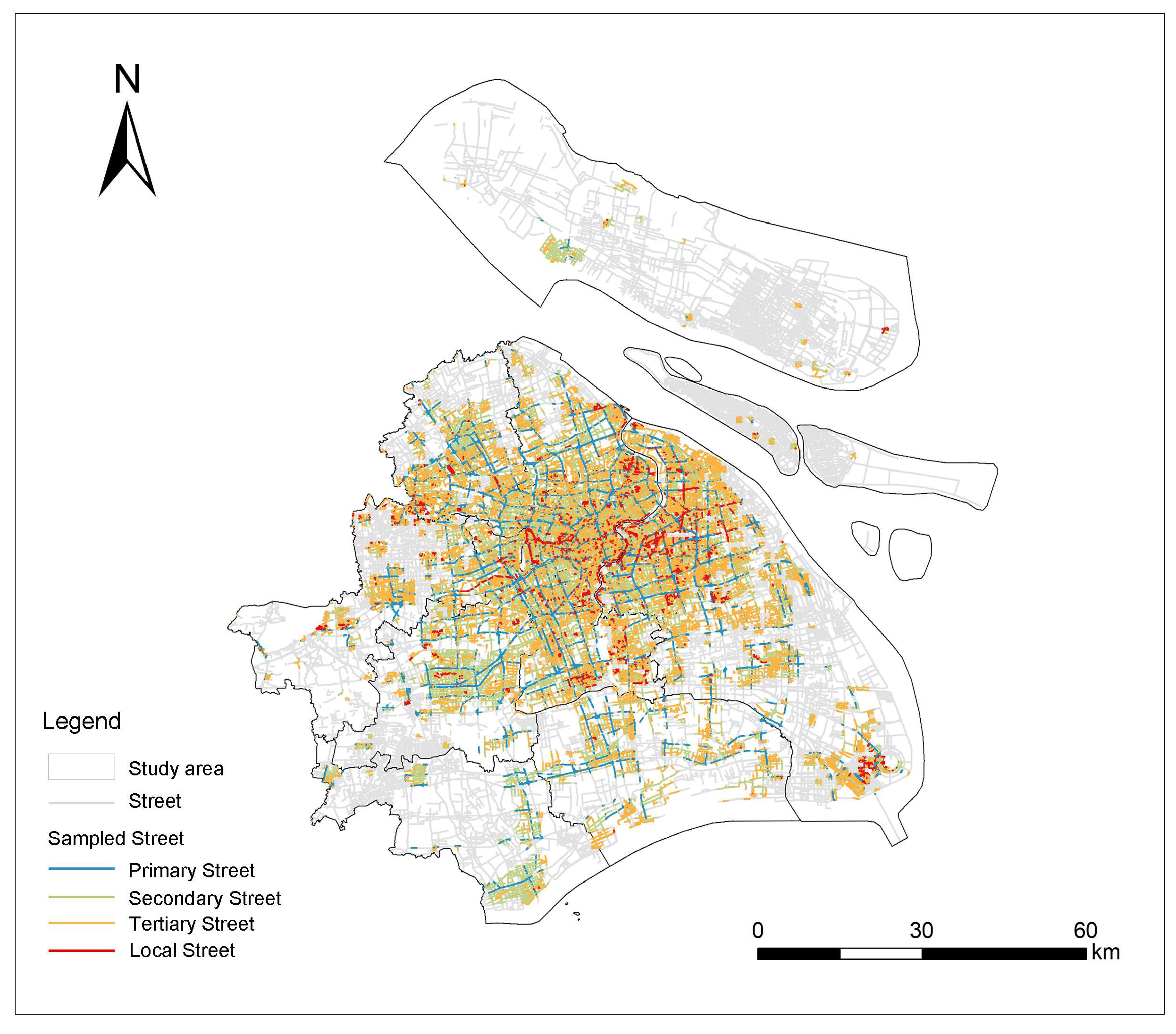
Shanghai is one of the most highly urbanized cities in China and features one of the most complex industrial structures [52]. It is characterized by the coexistence of multiple industrial tiers, including traditional manufacturing, services, and high-tech industries. As of 2024, Shanghai’s GDP reached RMB 5392.671 billion, marking a year-on-year growth of 5.0%. The city’s permanent population stands at approximately 24.87 million, making it one of the most urbanized cities in the country [53]. Its primary, secondary, tertiary, and local streets form a highly interconnected urban street network (Figure 1), from which sampled streets were selected for analysis in this study. By analyzing the nonlinear relationships and effects between street-level BE characteristics and industrial patterns, Shanghai serves as a typical and representative empirical context for exploring industrial spatial preferences and their regulatory mechanisms under the backdrop of rapid urbanization.

3.2. Data Source

3.2.1. Panoramic SVIs

The panoramic SVI used in this study was acquired through the Baidu API, which captures 360° panoramic SVI at each sampling point. In 2024, a total of 306,130 SVIs were successfully collected. During the data acquisition process, the sampling interval was set to 20 m, with a field of view of 360° and a heading angle of 0°, ensuring comprehensive coverage of street environment information.

3.2.2. Industrial Data

Measuring industrial agglomeration requires focusing on the core nodes of Shanghai’s industrial chain, its competitive advantages, and its emerging industry clusters, which provide a representative foundation for analyzing spatial clustering patterns [54]. To capture these key firms, we first identified relevant enterprise categories following the official classification framework issued by the Shanghai Municipal Commission of Economy and Informatization (SMCEI), which recognizes manufacturing single champion enterprises, A-share, HK-share, US-listed companies, specialized and innovative innovative Little Giant Enterprises (LGEs), technology-based small and medium-sized enterprises (SMEs), and national high-tech enterprises. We then accessed official public announcements and government-approved enterprise directories published by SMCEI (https://www.sheitc.sh.gov.cn/, accessed on 13 August 2025), ensuring the inclusion of authoritative and updated lists.

3.2.3. Auxiliary Data

We introduced three key macroeconomic variables covering the economic, social, and spatial dimensions: GDP, PD, and accessibility, all with a spatial resolution of 1 km × 1 km. The GDP and PD data were obtained from WorldPop (https://www.worldpop.org/, accessed on 13 August 2025). The accessibility indicator was derived using the locations of bus and metro stations provided by Baidu Maps (https://map.baidu.com/, accessed on 13 August 2025) and calculated as the number of transit stations within each grid cell using ArcGIS 10.8.1.

3.3. Data Processing

3.3.1. SBE Data

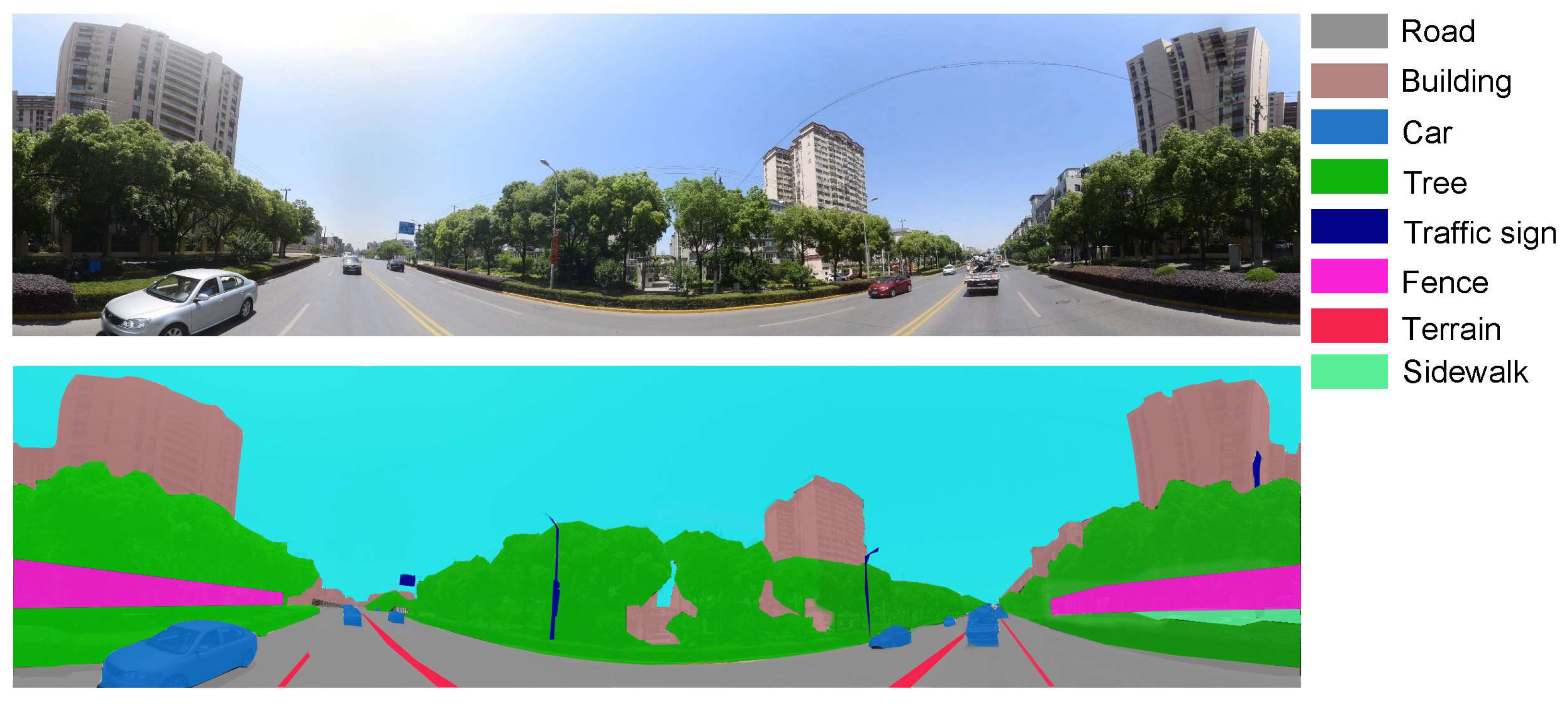
In the street view image processing stage, previous studies have demonstrated the effectiveness of Deeplab V3+ for streetscape semantic segmentation [55]. Therefore, this study employed Deeplab V3+, combined with the pretrained ADE20K dataset, to perform semantic segmentation on the collected SVI. This approach automatically identifies and extracts over one hundred categories of streetscape and environmental elements, including buildings, natural features, road facilities, street furniture, vehicles, and pedestrians (see Figure 2 for a representative semantic segmentation example). We selected the average proportions of Building, Sky, Tree, and Road as key indicators to represent the enclosure, greenness, and hardscape characteristics of the street space [56].

Table 2. The information on street scenes.

Variables (Target)	Description	Descriptive Statistics
		Mean	Min	Max
Building	Percentage of building, wall, and fence in the unit.	0.080	0.00	0.650
Sky	Percentage of sky elements in the street view image.	0.220	0.00	0.810
Tree	Percentage of vegetation in the unit reflecting greening level and visual comfort.	0.100	0.00	0.750
Road	Percentage of road in the unit.	0.010	0.00	0.300

summarizes the descriptive statistics of these selected streetscape variables, providing an overview of their distribution across the sampled units. These variables serve as the micro-level BE indicators in our subsequent modeling analysis.

For the BE characteristics, we selected seven core indicators: building density, building height, green ratio, impervious surface fraction, NDVI, water ratio, and SVF. These indicators comprehensively reflect the enclosure, three-dimensional morphology, greenness, ecological elements, and thermal environment characteristics of street spaces, effectively capturing the physical support and constraints of urban spatial structure on industrial agglomeration [35]. Details of all indicators and corresponding information are provided in Table 2. BD, BH, GR, ISF, NDVI, and WR were derived using Landsat 8 and Sentinel-2 remote sensing imagery, along with GlobeLand30 land cover data. The SVF was calculated in QGIS based on building footprints and BH data.

Table 3. Variable description and descriptive statistics of variables.

Variables (Target)	Description	Descriptive Statistics
		Mean	Min	Max
Building Density	Calculated as the total built-up floor area within each 1 km × 1 km grid cell.	0.10	0	0.45
Building Height	Average building height aggregated at the 1 km × 1 km grid level.	14.76	3	156
Green Ratio	Proportion of green cover area relative to the total land area in each 1 km × 1 km grid.	0.24	0	0.86
Impervious Surface Fraction	Fraction of impervious surfaces (e.g., roads, pavements) within the 1 km × 1 km grid cell.	0.65	0	0.99
Normalized Difference Vegetation Index	Mean NDVI value calculated for each 1 km × 1 km grid to indicate vegetation greenness.	0.47	0	0.88
Water Ratio	Proportion of surface water area within the 1 km × 1 km grid cell.	0.09	0	2.98
Sky View Factor	Average sky view factor derived for each 1 km × 1 km grid, representing street-level openness.	0.96	0.01	1.0

provides a detailed description and descriptive statistics of these indicators, highlighting their distributional characteristics across all spatial grids in the study area.

3.3.2. Shanghai Industrial Data

Nearly all companies, enterprises, and related facility points in China—including those not formally registered in the national industrial and commercial system, such as individual businesses or service outlets—can be geolocated through government-approved online map services [57]. Accordingly, this study first employed web scraping techniques to extract firm location data and geographic coordinates for the Shanghai area from Baidu Maps (https://map.baidu.com/, accessed on 13 August 2025). Subsequently, these points were matched and categorized by cross-referencing with the Chinese enterprise directories released by the Shanghai Municipal Commission of Economy and Informatization. The classified lists include manufacturing champions, A-share, HK-share, and US-listed companies, LGEs specialized and innovative firms, technology-based SMEs, and national high-tech enterprises. The final sample comprises 42,442 enterprises across seven categories, with detailed descriptive statistics presented in

Table 4. Descriptive statistics of enterprise categories in the sample.

Categories	Description	Descriptive Statistics
		Count	Ratio (%)
Manufacturing Single Champion Enterprises	Leading manufacturers dominating niche markets.	37	<0.10
US-listed Companies	Chinese firms listed on US stock exchanges.	41	<0.10
Hong Kong-listed Companies	Companies listed on the Hong Kong Stock Exchange.	155	0.40
A-share Listed Companies	Firms listed on mainland China’s A-share market.	418	1.00
Specialized and Innovative “Little Giant” Enterprises	SMEs recognized for specialization and innovation.	687	1.60
Technology-based Small and Medium-sized Enterprises	Small and medium firms with strong technological potential.	17,090	40.30
National High-tech Enterprises	Certified firms with advanced R&D and technology.	24,014	56.60

. It is worth noting that these firms represent core segments of Shanghai’s industrial chain, its competitive strengths, and its emerging industry clusters. Therefore, these companies not only exhibit significant economies of scale and spillover effects but also reflect the region’s innovation capacity and future growth potential [23].

3.4. Research Framework

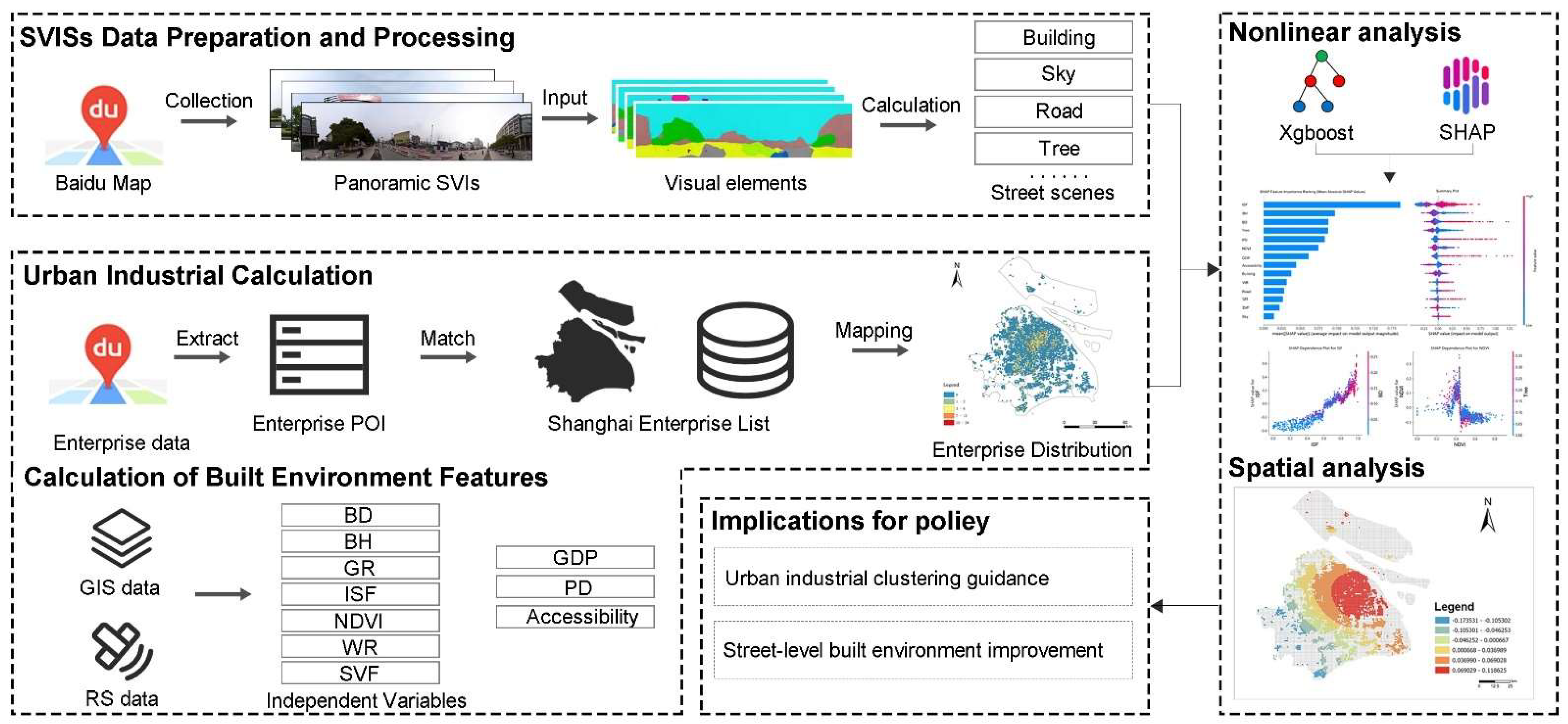
The data collection for this study covers four main dimensions: industrial data compilation, SVI acquisition, environmental indicator integration, and spatial data matching. Specifically, industrial statistics were primarily sourced from the Shanghai enterprise directories, providing the foundational dataset for constructing the spatial distribution of industries. To support fine-scale spatial analysis, a 1 km × 1 km fishnet grid was constructed across Shanghai, resulting in 3808 grid cells, each of which served as the basic unit of analysis [51]. Second, Python-based web scraping was used to obtain SVIs from Baidu Maps. Third, we employed DeepLab V3+ together with the ADE20K pretrained scene parsing dataset to extract elements from the street view images for semantic segmentation. An optimized formula was then applied to calculate streetscape visual perception indicators. This multi-dimensional measurement of environmental features provides robust data support for a comprehensive description of SBE characteristics. Subsequently, we constructed an XGBoost machine learning model to predict firm agglomeration and applied SHAP interpretability analysis to quantify the contribution of each environmental factor, thereby identifying the key drivers of firm spatial clustering. In parallel, the MGWR method was used to capture the local spatial heterogeneity patterns. Finally, combining model predictions with feature importance analysis, this study proposes neighborhood-level BE improvement strategies aimed at optimizing firm agglomeration, providing scientific decision-making support for enhancing business investment and improving urban spatial governance. The overall analytical logic and procedures of this study are illustrated in Figure 3, which presents the complete research framework encompassing data acquisition, variable construction, model analysis, and the formulation of optimization strategies.

3.4.1. Interpretable Machine Learning Algorithm

We employed the XGBoost algorithm to capture the complex nonlinear relationships between SBE characteristics and industrial patterns. XGBoost is an optimized implementation of the gradient boosting framework that supports parallel computation and is well-known for its high computational efficiency and prediction accuracy, making it particularly suitable for analyzing large-scale spatial datasets. The model was implemented using the XGBoost and Scikit-learn libraries in Python 3.9. The dataset was divided into a training set (70%) and a test set (30%). The loss function was set as mean squared error (MSE), assuming a convex objective function. In addition, a combination of grid search and five-fold cross-validation was applied to identify the optimal hyperparameters and to reduce the risk of model overfitting, ensuring the robustness and generalizability of the prediction results. The XGBoost model is represented as follows:

$$L(\Phi )={\sum }_{n=1}^N l(y_i^{\prime },y_i)+{\sum }_k \Omega (f_k)$$

(1)

where $l(y_i^{\prime },y_i)$ is the loss function measuring the difference between predicted and true values, and $\Omega \left(f_k\right)$ is the regularization term that penalizes the complexity of the model to improve generalization. The objective function $L(\Phi )$ combines both components to achieve a balance between model accuracy and simplicity.

We applied the SHAP (SHapley Additive exPlanations) method—an interpretable machine learning approach—to explain the global and local predictions of the XGBoost model and to uncover nonlinear effects and variable interactions. SHAP is based on the Shapley value from cooperative game theory, which quantifies the marginal contribution of each feature to a specific prediction and allocates fair influence values under different feature combinations. Specifically, we used the TreeExplainer tool from the SHAP package in Python 3.9 to interpret the model outputs, calculating both the global mean feature importance and the local prediction contributions. In addition, we extracted Shapley interaction values to evaluate the interaction synergy among variables in shaping urban industrial patterns. The Shapley model is expressed as follows:

$${\mathrm{\varnothing }}_j={\sum }_{S\subseteq \left\{x_1,\dots ,x_p\right\}\setminus \left\{x_j\right\}} {\displaystyle \frac{\left|S\right|!(p-|S|-1)!}{p!}}\left(f_x\left(S\cup \left\{x_j\right\}\right)-f_x\left(S\right)\right)$$

(2)

where ${\mathrm{\varnothing }}_j$ denotes the Shapley value for feature $x_j$, which quantifies its average marginal contribution across all possible feature coalitions.

3.4.2. Spatial Analysis

To further characterize the spatial heterogeneity effects of BE features on the target variables, we employed the MGWR model. Compared to traditional GWR, MGWR allows different independent variables to operate at varying spatial scales, thereby enabling a more precise capture of local and global effect differences and reflecting the multi-scale spatial characteristics of BE influences. The MGWR model is expressed as follows:

$$y_i={\beta }_0(u_i,v_i)+{\sum }_{k=1}^m {\beta }_k(u_i,v_i,b{w}_k)x_{ik}+{\epsilon }_i$$

(3)

where $y_i$ is the dependent variable, and ${\beta }_k(u_i,v_i,b{w}_k)$ represents the local regression coefficients that vary across spatial locations $(u_i,v_i)$ with different bandwidths $b{w}_k$. MGWR allows each explanatory variable to operate at its own spatial scale, thereby capturing spatial heterogeneity more flexibly than traditional GWR.

4. Results

As shown in Figure 4 (left), various types of innovative and high-growth firms in Shanghai exhibit a clear core–periphery spatial pattern. High-density clusters are mainly concentrated in the city center, major business districts, and industrial parks, while secondary clusters extend in a belt-like form along major transportation corridors. In contrast, peripheral areas show a scattered, low-density distribution, indicating that innovation-driven economic activities are highly concentrated in the urban core, with surrounding areas providing space for spillover and industrial upgrading. Meanwhile, as shown in Figure 4 (right), the distribution of street view images demonstrates a similar pattern, with higher coverage density in the core areas, major roads, and commercial centers. In suburban and rural areas, however, sparse road networks and weaker infrastructure result in limited street view data, which constrains fine-grained spatial analysis. Therefore, this study focuses on areas with complete and consistent coverage of street view images and BE data, while excluding peripheral zones with substantial data gaps. This approach helps ensure spatial comparability and reliability of results, providing a more robust understanding of how street-level BE features relate to industrial clustering.

Prior to constructing the XGBoost model, a Pearson correlation analysis was conducted to eliminate variables with excessively high correlation coefficients (Figure 5). The results indicate that most variables exhibit low to moderate correlations, with no pairwise correlation coefficients exceeding 0.7, suggesting that there is no severe multicollinearity. A relatively strong positive correlation was observed between BD and ISF (r = 0.68) and between BD and ISF (r = 0.68), while a notable negative correlation was found between ISF and NDVI (r = −0.62).

4.1. Nonlinear Contributions and Interaction Effects

The XGBoost model hyperparameters were systematically optimized using a Bayesian optimization framework implemented through the Optuna library. We employed a Tree-structured Parzen Estimator (TPE) sampler to efficiently explore the hyperparameter search space, which included eight critical parameters: n_estimators (100–1000), max_depth (3–10), learning_rate (0.01–0.3, log-distributed), subsample (0.6–1.0), colsample_bytree (0.6–1.0), reg_alpha (1 × 10⁻⁴ to 1.0, log-distributed), reg_lambda (1 × 10⁻³ to 5.0, log-distributed), and min_child_weight (0.5–10). The optimization process was conducted over 50 trials with 5-fold cross-validation, using the coefficient of determination (R²) as the objective function to maximize. To ensure robust parameter estimation and prevent overfitting, we implemented stratified cross-validation with consistent random seeds (random_state = 2021) across all experimental procedures.

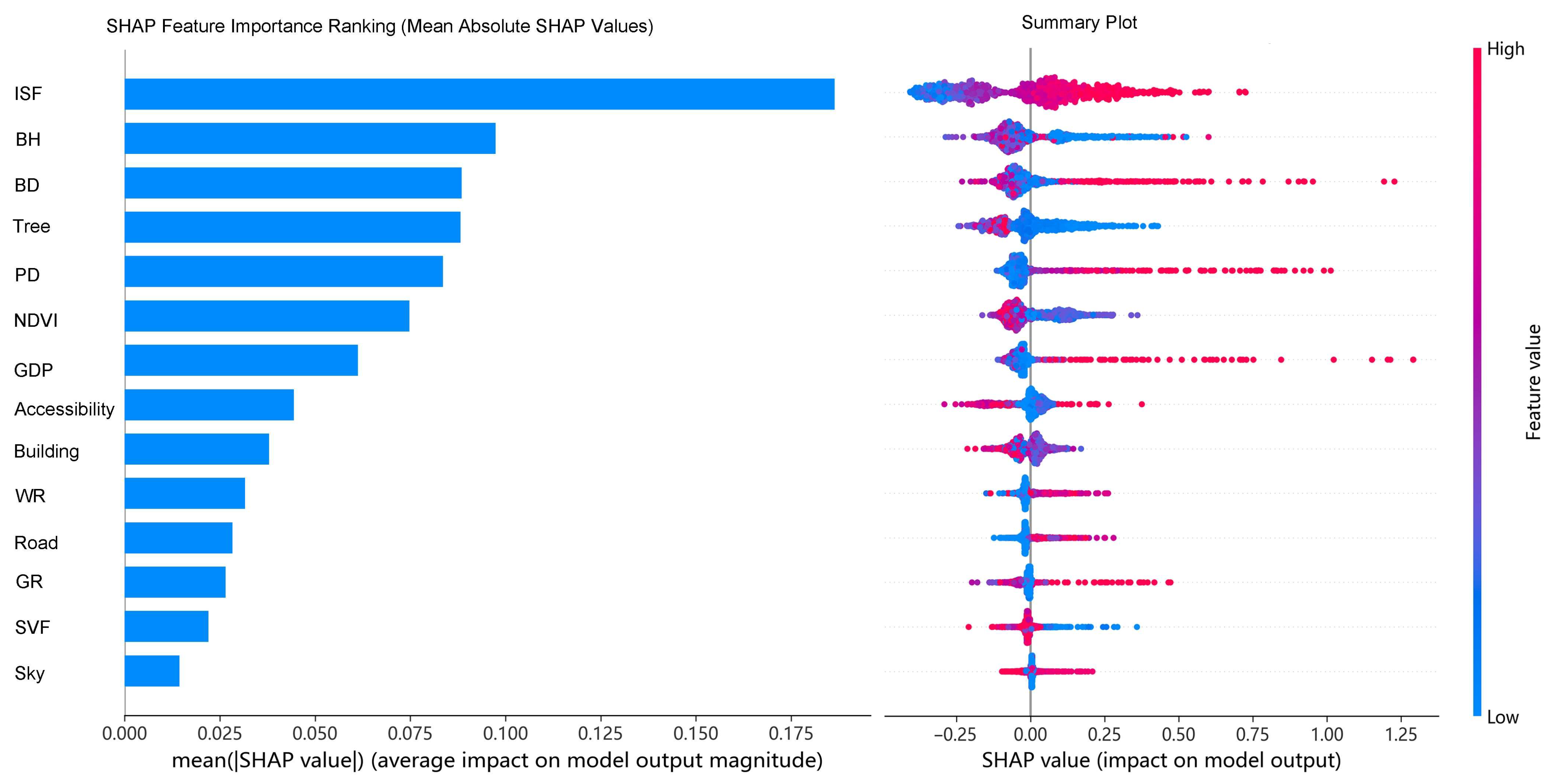
The model’s predictive performance was evaluated using root mean square error (RMSE), mean absolute error (MAE), and R-squared (R²), as summarized in

Table 5. Model performance.

	Number	MAE	MSE	RMSE	R2
Train dataset	2666	0.10	0.018	0.14	0.74
Test dataset	1142	0.11	0.025	0.15	0.68

. Figure 6 illustrates the feature importance ranking generated by XGBoost, with BD, Building, and ISF emerging as the top three influential variables, followed by BH, WR, SVF, Tree, Sky, NDVI, GR, and Road. To interpret the contribution and directionality of each predictor, SHAP (SHapley Additive exPlanations) values were further employed, providing robust insights into the nonlinear effects of the BE on industrial clustering.

To identify the key features influencing firm agglomeration, this study used SHAP to rank the relative importance of the contributing factors (Figure 6). The left side of the figure shows the importance of various BE factors along with their specific relative contributions, which are ranked in descending order of importance. On the right, the contribution of each factor to urban vitality is highlighted, with the color gradient ranging from red to blue to reflect high to low feature values. The SHAP values along the horizontal axis indicate the negative or positive impacts on firm agglomeration.

Among the BE and urban fundamental variables, ISF exhibits the most significant positive effect on firm agglomeration, ranking first in overall importance. Morphological attributes of the BE, particularly BH and BD, rank second and third, respectively, highlighting the critical roles of vertical scale and spatial compactness in shaping firm clustering patterns. Tree and Building, derived from street-level imagery, rank in the middle tier of all evaluated variables, indicating a moderate level of importance in shaping firm agglomeration outcomes. PD, GDP, accessibility, and WR also appear within the upper half of the importance ranking, reflecting their relatively stronger relevance compared to other factors. In contrast, vegetation-related indicators such as NDVI and GR are ranked lower, suggesting a more limited contribution to the model’s predictive performance. Variables including Sky, SVF, and Road are positioned at the bottom of the ranking, indicating minimal overall influence on firm agglomeration in this context.

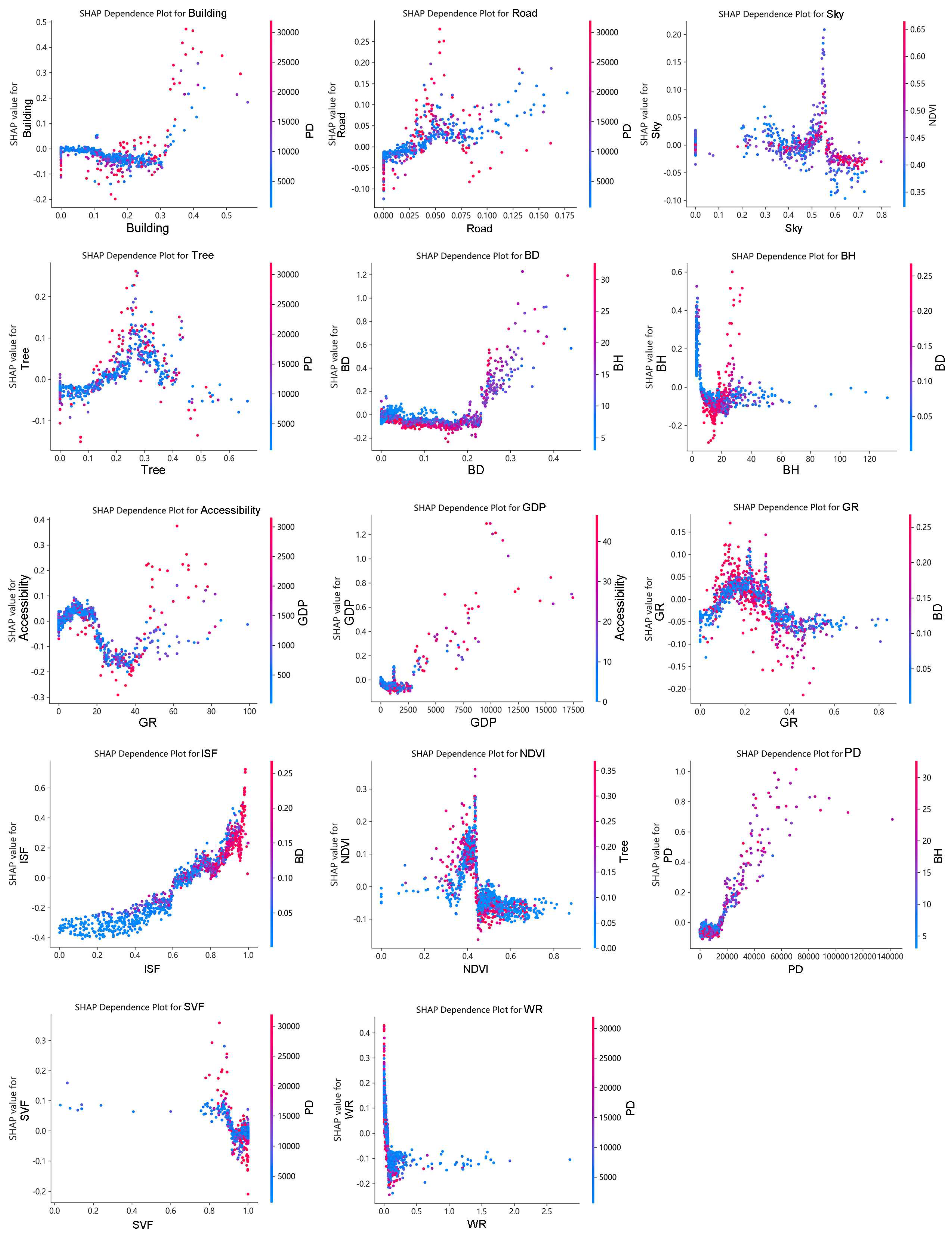
Figure 7 represents the SHAP dependence plots for each built environment variable, aiming to reveal the nonlinear patterns of their marginal contributions to firm agglomeration across different value ranges. The x-axis represents the actual values of each variable, while the y-axis shows the corresponding SHAP values. The color gradient indicates changes in another potential interacting variable, facilitating the identification of possible interaction effects and joint mechanisms.

Among the top-ranked variables, Tree and PD exhibit pronounced nonlinear influence patterns. Tree coverage displays a U-shaped relationship: its contribution to firm agglomeration is limited—or even negative—at lower levels but increases sharply once it exceeds a threshold of approximately 0.2. This suggests that green infrastructure becomes a positive driver of agglomeration only when reaching a certain scale, particularly when combined with compact urban morphology. The color gradient further reveals an interaction with BD, indicating a synergistic effect between greening and spatial compactness in shaping firm location preferences. Similarly, the SHAP dependence plot for PD reveals a clear threshold effect. At low to moderate levels, PD exerts minimal impact on agglomeration. However, once population density surpasses approximately 40,000, the SHAP values increase markedly. This pattern reflects the benefits of economies of scale and market accessibility in high-density environments, although the steep rise may also imply potential spatial saturation, warranting further investigation. In addition, both BH and BD exhibit distinct nonlinear patterns with abrupt shifts. For instance, the SHAP value for BH increases significantly once building height exceeds roughly 60 m, aligning with the vertical clustering tendency of central business districts. BD shows negligible influence at lower levels but becomes a strong positive contributor once surpassing 0.2, reaffirming the positive role of spatial compactness in facilitating firm agglomeration.

4.2. Spatial Mechanisms of SBE Effects on Firm Agglomeration

4.2.1. Spatial Autocorrelation Results

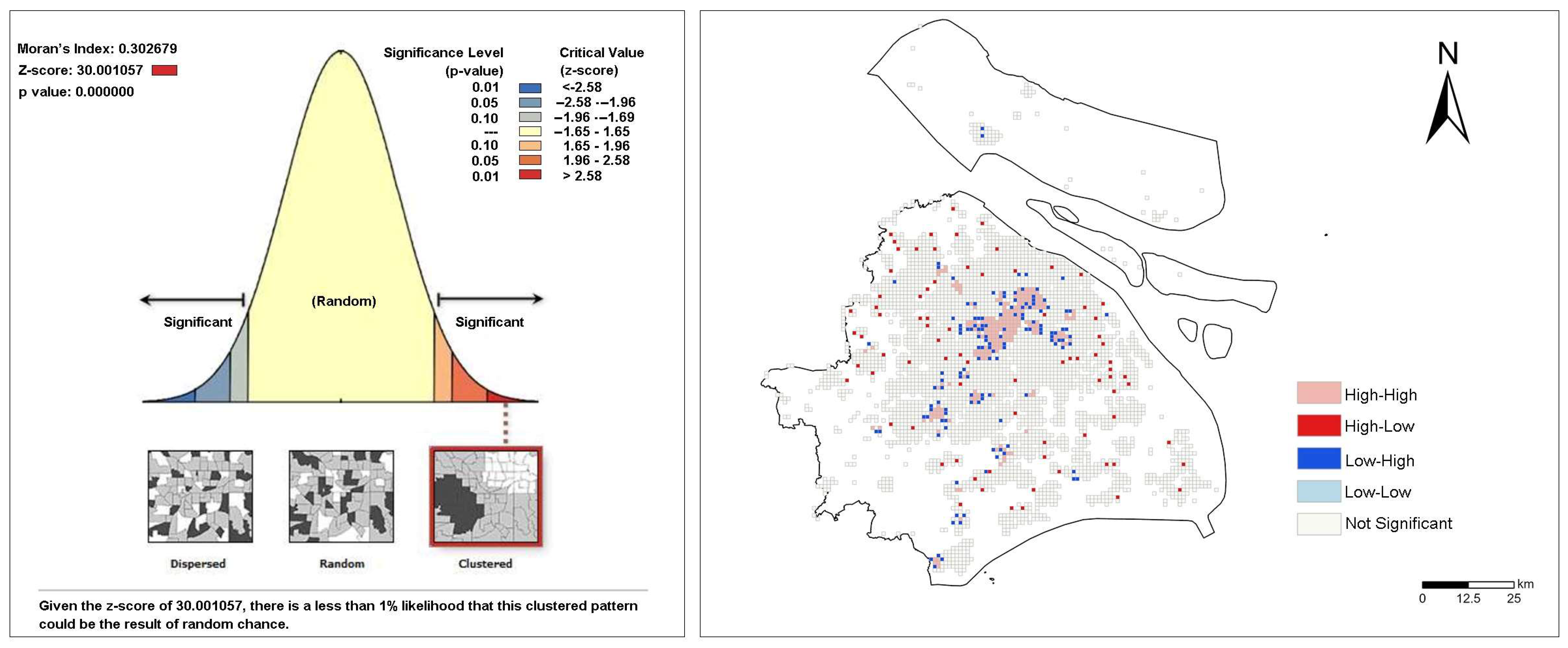
We first confirmed the presence of significant spatial autocorrelation in firm agglomeration using the Global Moran’s I and Local Moran’s I (LISA) tests (Figure 8). The Global Moran’s I value was 0.3027 with a Z-score of 30.0011 (p < 0.01), indicating a highly significant clustered pattern rather than a random distribution. The LISA results further reveal high-high clusters in core urban areas and low-low clusters, along with a few spatial outliers, in peripheral areas. Subsequently, an OLS regression model was established as the baseline, and prior to the regression, multicollinearity among explanatory variables was assessed using the Variance Inflation Factor (VIF) test (Appendix A), with all VIF values found to be below the threshold of 5 (maximum = 3.918), indicating no serious multicollinearity. Therefore, no variables were removed on this ground. Table 5 shows that MGWR regression results are more accurate than those from OLS and GWR.

In the subsequent MGWR model analysis, we retained all 14 explanatory variables. This decision was based not only on the absence of multicollinearity among variables, but also on the consideration that some variables with relatively low global feature importance may exhibit spatially heterogeneous effects that are not readily captured by global analyses.

4.2.2. MGWR Results

Table 6. Comparison of OLS, GWR, and MGWR models.

Regression Model	AICc	R2	Adj.R2
OLS	13,896.953	0.142	0.159
GWR	10,072.934	0.468	0.457
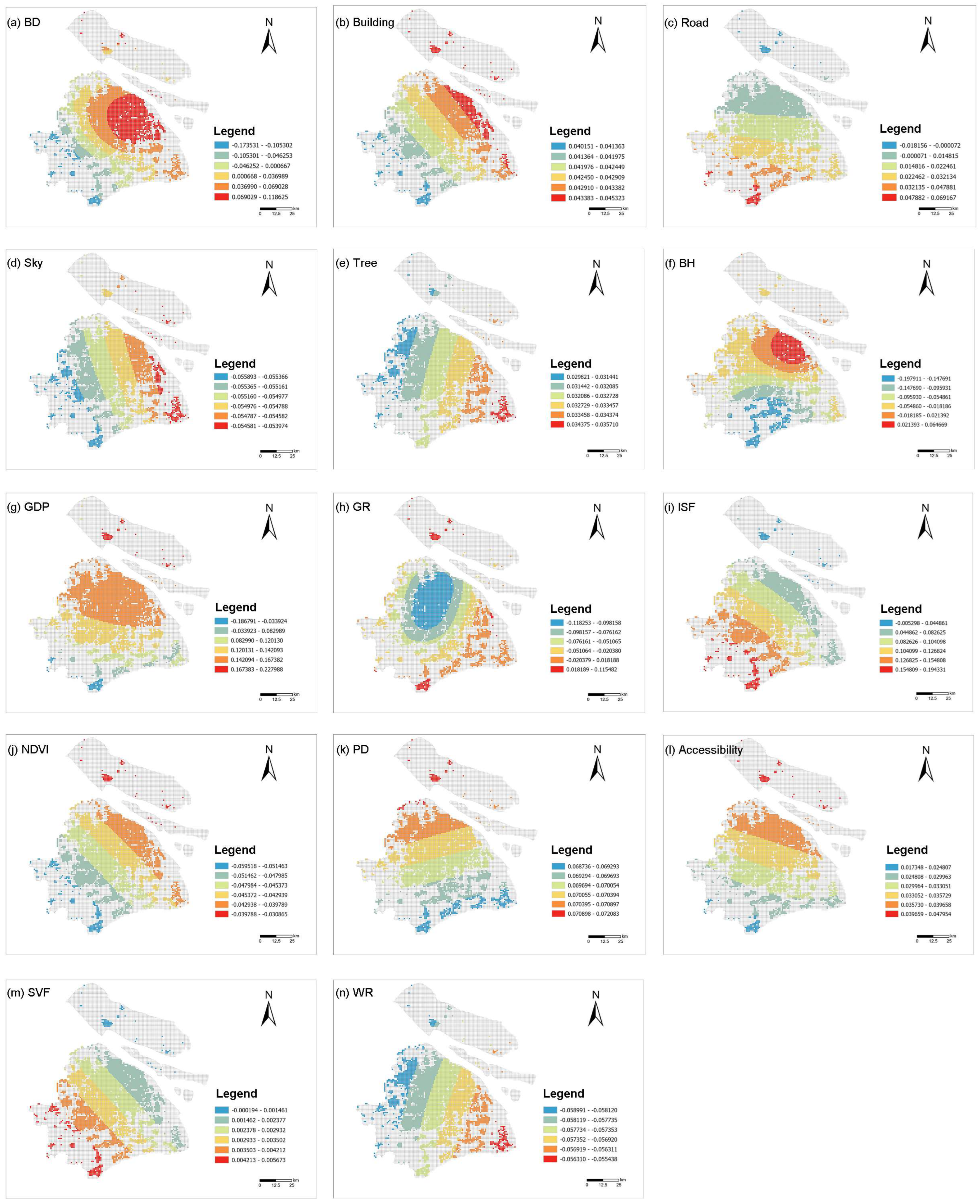
MGWR	10,074.259	0.571	0.562

presents a comparative assessment of the OLS, GWR, and MGWR models, demonstrating that MGWR delivers superior overall performance by explicitly capturing spatially varying relationships between predictors and firm agglomeration. The detailed results of MGWR are reported in

Table 7. MGWR regression results.

Variables	Bandwidth	Minimum Value	Median	Maximum Value	Average Value
BD	40,496.91 (20.88)	−0.1735	0.0441	0.1186	0.0267
BH	40,496.91 (20.88)	−0.1979	−0.041	0.0647	−0.0517
GR	40,496.91 (20.88)	−0.1183	−0.0745	0.1155	−0.064
ISF	62,890.08 (32.42)	−0.0053	0.1029	0.1943	0.1053
NDVI	135,355.89 (69.78)	−0.0595	−0.0452	−0.0309	−0.0455
WR	193,981.96 (100.00)	−0.059	−0.0576	−0.0554	−0.0575
SVF	193,981.96 (100.00)	−0.0002	0.0029	0.0057	0.0029
Building	193,981.96 (100.00)	0.0402	0.0426	0.0453	0.0426
Sky	193,981.96 (100.00)	−0.0559	−0.055	−0.054	−0.055
Tree	193,981.96 (100.00)	0.0298	0.0324	0.0357	0.0325
Road	76,729.82 (39.56)	−0.0182	0.0187	0.0692	0.0204
Accessibility	99,122.98 (51.10)	0.0173	0.0341	0.048	0.0336
PD	193,981.96 (100.00)	0.0687	0.0701	0.0721	0.07
GDP	60,870.89 (31.38)	−0.1868	0.1447	0.228	0.1323

Bandwidth indicates the optimal spatial bandwidth (in meters); values in parentheses represent the proportion of total observations, reflecting spatial heterogeneity.

and illustrated in Figure 9. As can be seen, the variable bandwidth provides a more precise and comprehensive perspective for exploring the relationships of spatial data. The optimal bandwidths for MGWR were determined using a Golden Section Search procedure to minimize AICc values [58]. Based on a comparative assessment (Appendix A,

Table A2. Comparison of Model Performance between Bisquare and Gaussian Kernels in MGWR.

Kernel Function	AICc	R2	Adj. R2	Bandwidth Selection Method
Bisquare	10,074.109	0.571	0.562	Golden Section Search
Gaussian	10,074.259	0.434	0.414	Golden Section Search

), the bisquare kernel outperformed the Gaussian kernel in terms of AICc and R² values, and was therefore adopted for the final MGWR estimations. All spatial analyses and data processing were conducted using ArcGIS 10.8.1 and ArcGIS Pro 3.5.

Table 7 summarizes the local regression coefficient distributions of the MGWR model, highlighting the spatial heterogeneity and threshold effects of different explanatory variables on firm agglomeration. Among all predictors, GDP (mean coefficient = 0.1323, bandwidth = 31.38%) emerges as one of the strongest and most spatially varying drivers. Its positive influence is pronounced in core urban areas (maximum 0.228), indicating that robust economic fundamentals substantially enhance firm clustering, while some peripheral zones show weakly negative effects, possibly due to structural mismatches between economic activity and industrial land availability.

ISF (mean = 0.1053, bandwidth = 32.42%) is another key factor, displaying strong positive effects in high-intensity built-up zones (max 0.1943), suggesting that developed hard surfaces are closely associated with agglomeration economies. Similarly, BD (mean = 0.0267, bandwidth = 20.88%) shows predominantly positive contributions (max 0.1186) in central areas, but its effect reverses to negative in some peripheral grids (min −0.1735), implying congestion thresholds beyond which additional density suppresses clustering. BH (mean = −0.0517, bandwidth = 20.88%), while significant in many locations, generally exhibits negative coefficients, reflecting potential diseconomies of excessive vertical development at the micro-scale.

Accessibility-related variables also play a major role. Accessibility (mean = 0.0336, bandwidth = 51.10%) has stable positive effects across the region (max 0.048), especially along major transport corridors, reinforcing its importance in supporting firm location choices. Road (mean = 0.0204, bandwidth = 39.56%) contributes positively in most core areas (max 0.0692), but negative local effects in some suburban zones (min −0.0182) suggest that over-fragmented road networks may undermine clustering benefits.

Ecological variables exhibit mixed effects. GR (mean = −0.064) and NDVI (mean = −0.0455) both reveal inverted U-shaped patterns: moderate greenery enhances spatial attractiveness (GR max = 0.1155), while excessive ecological coverage can displace developable land and dampen clustering. Tree coverage (mean = 0.0325) shows a small but consistently positive effect, while WR (mean = −0.0575) has a weak negative influence throughout the study area.

Other built environment perceptual features exert relatively minor effects. Building facade visibility (mean = 0.0426) has a stable positive association, whereas SVF (SVF, mean = 0.0029) and Sky (mean = −0.055) contribute little explanatory power, indicating that visual openness plays a negligible role in firm location decisions compared to economic, density, and accessibility factors. PD remains globally positive (mean = 0.07, bandwidth = 100%), reflecting stable labor market effects without spatial heterogeneity. Figure 9 further visualizes the local regression coefficient distributions of the above variables, intuitively illustrating their spatial heterogeneity and the geographic patterns of effect intensity.

5. Discussion

5.1. Nonlinear Effects of Street-Level Built Environment on Urban Industrial Agglomeration

This study comprehensively examines the influence of macroeconomic factors, streetscape perceptual features, and built environment characteristics on urban industrial agglomeration, revealing pronounced nonlinear effects and spatial heterogeneity. The observed nonlinear relationships indicate that the formation of urban industrial spatial patterns is not solely determined by the overall levels of built environment variables, but rather by whether these variables exceed specific threshold values. This finding contrasts sharply with the simplified assumptions commonly made in previous linear studies [23].

5.1.1. Relative Importance of Environmental Variables for Urban Firm Agglomeration

Among all micro-scale built environment variables, ISF, BH, and BD exhibit the strongest explanatory power, highlighting the critical role of spatial intensity and compactness in fostering the agglomeration of strategic emerging industries. Notably, BH demonstrates a negative association with firm clustering, while ISF and BD show positive correlations. This suggests that firms favor spatial intensity primarily characterized by high ground-level development density and compact horizontal configurations, rather than vertical expansion alone. This finding contrasts with the assertion by Li et al. that “vertical urbanism promotes innovation-driven agglomeration” [59], indicating that strategic emerging industries may prefer flexible and open spatial arrangements over purely high-rise environments.

Notably, although both the street-level Tree variable and the remotely sensed NDVI are conventionally perceived as enhancing urban environmental attractiveness, the present study finds that their overall effects on firm agglomeration are negative. This result challenges the traditional assumption that “urban greening is always a positive externality” [28], suggesting that areas with high vegetation coverage may be associated with lower development intensity or spatial conflicts that hinder firms’ access to transportation, clientele, and supporting services—factors critical for the growth of strategic emerging industries. Furthermore, the negative effect of Tree may reflect its obstructive role at the street level, reducing visual exposure, signage visibility, and spatial efficiency.

Additionally, macroeconomic variables such as PD and GDP exhibit greater explanatory power than accessibility. This may be attributed to the high spatial coupling between economic activity and population distribution in megacities such as Shanghai, which collectively underpin the foundations for industrial development [60]. In contrast, accessibility exerts a relatively weaker influence in such infrastructure-rich contexts, likely due to its spatially homogeneous distribution [61].

5.1.2. Nonlinear Effects of Environmental Variables on Urban Firm Agglomeration

The SHAP analysis conducted in this study reveals pronounced nonlinear effects, most notably an inverted U-shaped relationship between Tree coverage and NDVI and their influence on firm agglomeration. Specifically, the SHAP value for Tree peaks at 0.11 when the perceived tree coverage rate reaches approximately 0.25. Beyond this threshold, further increases in greenery are associated with a declining probability of firm clustering. This finding partially supports the “optimal greenness” hypothesis proposed by Karusisi, yet the post-threshold negative effect is more pronounced in our study [62], indicating that strategic emerging industries may be less tolerant of excessive greening than previously suggested in resident-based preference studies. Moreover, SHAP interaction effects reveal a negative interaction between Tree and NDVI, suggesting that micro-scale greening strategies (e.g., green walls, rooftop vegetation) may better align with the spatial and operational needs of strategic emerging industries than broad-scale vegetation coverage captured by NDVI. This scale mismatch may reflect underlying spatial conflicts and competitive dynamics in land use planning for industrial zones. Accessibility also demonstrates an inverted U-shaped pattern, with the marginal contribution to firm agglomeration peaking at approximately 50 transit stops per square kilometer. Beyond this threshold, the marginal effect declines rapidly, possibly due to the emergence of negative externalities such as environmental stress and congestion, as observed in prior studies [38].

5.2. Spatial Heterogeneity of Industrial Agglomeration in Shanghai

The MGWR analysis reveals pronounced spatial heterogeneity in the effects of built environment and socio-economic variables on firm agglomeration. Notably, most streetscape perception variables—such as Tree, Sky, and Building—exhibit relatively stable spatial effects, with optimal bandwidths approaching the global level. This contrasts with earlier studies emphasizing strong spatial variation in streetscape variables [34]. Such consistency suggests a form of “visual consensus”, wherein these perceptual features exert relatively uniform influences in industry-oriented contexts, regardless of spatial location.

In contrast, variables such as GR, NDVI, GDP, ISF, and accessibility exhibit marked spatial non-stationarity. In particular, NDVI and GR display significantly negative effects on firm agglomeration in central districts (e.g., Huangpu District, Jing’an District), while showing neutral or even positive associations in peripheral areas (e.g., Zhangjiang High-tech Park in Pudong New Area and Zizhu High-tech Zone in Minhang District). This divergence implies that the impact of green resources is context-dependent, varying with development intensity and functional orientation: in high-density urban cores, excessive greenery may constrain land use efficiency and development potential, whereas in peripheral zones, green infrastructure enhances environmental attractiveness and supports the growth of green manufacturing and biopharmaceutical industries.

These spatial patterns align with Shanghai’s current spatial development strategy of “multi-nodal agglomeration and differentiated growth” [11]. The urban core prioritizes land use optimization to accommodate high-density knowledge-intensive sectors such as AI and fintech, while peripheral zones leverage ecological advantages to attract green and emerging industries. This finding contributes to a more nuanced understanding of the trade-offs between firm siting and green space planning, offering actionable insights for place-based industrial policy and sustainable spatial planning.

5.3. Significance of This Study

Currently, both the academic community and urban policymakers face the pressing challenge of balancing high-density development with sustained industrial agglomeration in megacities. “High-quality spatial environments” and “innovation-driven development” are widely recognized as critical levers for enhancing urban competitiveness and promoting long-term sustainability. By integrating multi-source BE data with street view imagery (SVI)-derived perceptual features, this study employs interpretable spatial analysis techniques to systematically uncover the multi-dimensional effects of environmental variables across scales on urban firm clustering, as well as their spatial heterogeneity. This offers new theoretical insights and empirical evidence for addressing a key academic and policy concern.

For high-density metropolises such as Shanghai, optimizing the industrial spatial layout should not rely solely on intensive construction. Instead, it is essential to consider the threshold effects of building morphology, the appropriateness of local-scale greenery, and the synergistic roles of open space systems. In terms of policy design, particular attention should be paid to achieving a balance between building intensity and greenery in core urban areas to prevent environmental degradation caused by excessive compactness. In emerging functional zones, improving streetscape quality and enhancing multi-dimensional accessibility are key to stimulating the clustering potential of innovation-oriented firms. In peripheral low-density areas, it is crucial to guide industrial spillover while maintaining ecological integrity, thereby mitigating the risk of spatial “hollowing out.”

In sum, this study advocates for the coordinated optimization of physical environmental conditions, transportation accessibility, and perceptual landscape elements, aiming to construct a more resilient and adaptive innovation-oriented spatial network. Such a network can support urban economic transformation and provide a strategic foundation for sustainable regional development.

6. Conclusions

This study constructs an interpretable spatial machine learning framework based on multi-source urban data to systematically investigate the nonlinear effects and spatial heterogeneity of street-level BE features on firm agglomeration in Shanghai. By integrating XGBoost, SHAP, and MGWR methods, we effectively modeled complex variable interactions, identified critical threshold effects, and revealed significant spatial non-stationarity. The key findings are as follows: (1) Built morphology indicators such as ISF and BD significantly promote industrial agglomeration and exhibit clear threshold effects, while excessive BH may suppress clustering, suggesting that vertical development must align with local spatial adaptability. (2) Streetscape perception features such as Tree and Sky show relatively consistent “visual consensus” effects across space, whereas greenness indicators like NDVI and GR demonstrate context-dependent heterogeneity—suppressing agglomeration in high-density core areas but facilitating it in peripheral zones. (3) Both accessibility and greenness show inverted U-shaped relationships with firm clustering, indicating that while moderate levels are beneficial, exceeding certain thresholds may generate negative externalities such as congestion or inefficient resource allocation.

Theoretically, this study contributes to the urban economic geography and spatial planning literature by deepening our understanding of how micro-scale built environment factors shape industrial spatial structures. The integrated use of interpretable machine learning and geographically weighted regression validates the existence of variable interactions, threshold mechanisms, and spatial non-stationarity, enriching the analytical paradigm of industrial agglomeration research. Furthermore, it provides empirical grounding for an emerging urban spatial theory that integrates perception, morphology, and functionality.

Practically, the findings offer place-sensitive guidance for optimizing the built environment to promote the orderly development of high-tech industries in Shanghai. In central urban areas, policies should aim to control excessive building height, enhance ground-level development density and accessibility, and avoid over-greening that may hinder spatial efficiency. In emerging functional zones, emphasis should be placed on improving streetscape legibility and environmental perception to enable threshold-oriented spatial strategies. In low-density peripheral districts, ecological advantages should be leveraged to foster green industrial clusters, with enhanced connectivity and policy coordination strengthening spatial synergy with the urban core. Additionally, we advocate for the establishment of street-level built environment monitoring and dynamic evaluation systems to enable data-driven, precision-based industrial spatial planning and governance. These insights collectively provide robust scientific support for building a more resilient and adaptive urban innovation network.

References

1. Sgambati, S.; Gargiulo, C. The Evolution of Urban Competitiveness Studies over the Past 30 Years. A Bibliometric Analysis. Cities 2022, 128, 103811. [Google Scholar] [CrossRef]
2. Hu, R. Optimal Urban Competitiveness Assessment Using Cloud Computing and Neural Network. J. Cloud Comput. 2023, 12, 81. [Google Scholar] [CrossRef]
3. Luo, Y.; Shen, J. Urban Entrepreneurialism, Metagovernance and ‘Space of Innovation’: Evidence from Buildings for Innovative Industries in Shenzhen, China. Cities 2022, 131, 104067. [Google Scholar] [CrossRef]
4. Liu, H.; Gou, P.; Xiong, J. Vital Triangle: A New Concept to Evaluate Urban Vitality. Comput. Environ. Urban Syst. 2022, 98, 101886. [Google Scholar] [CrossRef]
5. Du, Z.; Hao, P. Firm Clustering, Agglomeration Externalities and Energy Efficiency: Evidence from Chinese Industrial Enterprises. Energy Econ. 2025, 145, 108451. [Google Scholar] [CrossRef]
6. Zeng, G.; Hu, Y.; Zhong, Y. Industrial Agglomeration, Spatial Structure and Economic Growth: Evidence from Urban Cluster in China. Heliyon 2023, 9, e19963. [Google Scholar] [CrossRef]
7. Miörner, J.; Zukauskaite, E.; Trippl, M.; Moodysson, J. Creating Institutional Preconditions for Knowledge Flows in Cross-Border Regions. Environ. Plan. C Politics Space 2018, 36, 201–218. [Google Scholar] [CrossRef]
8. Kim, S.; Woo, A. Streetscape and Business Survival: Examining the Impact of Walkable Environments on the Survival of Restaurant Businesses in Commercial Areas Based on Street View Images. J. Transp. Geogr. 2022, 105, 103480. [Google Scholar] [CrossRef]
9. Esmaeilpoorarabi, N. Place Quality in Innovation Clusters: An Empirical Analysis of Global Best Practices from Singapore, Helsinki, New York, and Sydney. Cities 2018, 74, 156–168. [Google Scholar] [CrossRef]
10. Zhang, S.; Yuan, C.; Wang, Y. The Impact of Industry–University–Research Alliance Portfolio Diversity on Firm Innovation: Evidence from Chinese Manufacturing Firms. Sustainability 2019, 11, 2321. [Google Scholar] [CrossRef]
11. Duan, J.; Zhao, Z.; Xu, Y.; You, X.; Yang, F.; Chen, G. Spatial Distribution Characteristics and Driving Factors of Little Giant Enterprises in China’s Megacity Clusters Based on Random Forest and MGWR. Land 2024, 13, 1105. [Google Scholar] [CrossRef]
12. Ye, Y.; Wu, K.; Xie, Y.; Huang, G.; Wang, C.; Chen, J. How Firm Heterogeneity Affects Foreign Direct Investment Location Choice: Micro-Evidence from New Foreign Manufacturing Firms in the Pearl River Delta. Appl. Geogr. 2019, 106, 11–21. [Google Scholar] [CrossRef]
13. Huang, D.; Xu, G.; Li, C.; Yang, S. Effects of High-Tech Industrial Agglomeration and Innovation on Regional Economic Development in China: Evidence from Spatial-Temporal Analysis and Spatial Durbin Model. Econ. Anal. Policy 2025, 86, 692–712. [Google Scholar] [CrossRef]
14. Peng, C.; Elahi, E.; Fan, B.; Li, Z. Effect of High-Tech Manufacturing Co-Agglomeration and Producer Service Industry on Regional Innovation Efficiency. Front. Environ. Sci. 2022, 10, 942057. [Google Scholar] [CrossRef]
15. Ge, L.; Li, C.; Sun, L.; Hu, W.; Ban, Q. The Relationship between High-Tech Industrial Agglomeration and Regional Innovation: A Meta-Analysis Investigation in China. Sustainability 2023, 15, 16545. [Google Scholar] [CrossRef]
16. Li, L.; Zhang, X. Spatial Evolution and Critical Factors of Urban Innovation: Evidence from Shanghai, China. Sustainability 2020, 12, 938. [Google Scholar] [CrossRef]
17. Growth, Innovation, Scaling, and the Pace of Life in Cities. Available online: https://www.pnas.org/doi/epdf/10.1073/pnas.0610172104 (accessed on 5 August 2025).
18. Esmaeilpoorarabi, N.; Yigitcanlar, T.; Guaralda, M.; Kamruzzaman, M. Does Place Quality Matter for Innovation Districts? Determining the Essential Place Characteristics from Brisbane’s Knowledge Precincts. Land Use Policy 2018, 79, 734–747. [Google Scholar] [CrossRef]
19. Xie, Y.; Zhang, J.; Li, Y.; Zhu, Z.; Deng, J.; Li, Z. Integrating Multi-Source Urban Data with Interpretable Machine Learning for Uncovering the Multidimensional Drivers of Urban Vitality. Land 2024, 13, 2028. [Google Scholar] [CrossRef]
20. Qiu, W.; Li, W.; Liu, X.; Zhang, Z.; Li, X.; Huang, X. Subjective and Objective Measures of Streetscape Perceptions: Relationships with Property Value in Shanghai. Cities 2023, 132, 104037. [Google Scholar] [CrossRef]
21. Koo, B.W.; Hwang, U.; Guhathakurta, S. Streetscapes as Part of Servicescapes: Can Walkable Streetscapes Make Local Businesses More Attractive? Comput. Environ. Urban Syst. 2023, 106, 102030. [Google Scholar] [CrossRef]
22. Carmona, M.; Gabrieli, T.; Hickman, R.; Laopoulou, T.; Livingstone, N. Street Appeal: The Value of Street Improvements. Prog. Plan. 2018, 126, 1–51. [Google Scholar] [CrossRef]
23. Wu, K.; Wang, Y.; Ye, Y.; Zhang, H.; Huang, G. Relationship Between the Built Environment and the Location Choice of High-Tech Firms: Evidence from the Pearl River Delta. Sustainability 2019, 11, 3689. [Google Scholar] [CrossRef]
24. Guo, X.; Guo, K.; Zheng, H. Industrial Agglomeration and Enterprise Innovation Sustainability: Empirical Evidence from the Chinese A-Share Market. Sustainability 2023, 15, 11660. [Google Scholar] [CrossRef]
25. Cui, L.; Shen, J.; Mai, Z.; Lin, C.; Wang, S. Spatial Distribution and Location Determinants of High-Tech Firms in Shenzhen, a Chinese National Innovative City. Land 2024, 13, 1355. [Google Scholar] [CrossRef]
26. Li, J.; Webster, D.; Cai, J.; Muller, L. Innovation Clusters Revisited: On Dimensions of Agglomeration, Institution, and Built-Environment. Sustainability 2019, 11, 3338. [Google Scholar] [CrossRef]
27. Marshall, A. Principles of Economics; Springer: Berlin/Heidelberg, Germany, 2013; ISBN 978-1-137-37526-1. [Google Scholar]
28. Krugman, P. Increasing Returns and Economic Geography. J. Political Econ. 1991, 99, 3. [Google Scholar] [CrossRef]
29. Wu, S.; Li, B.; Xu, D. Agglomeration Characteristics and Influencing Factors of Urban Innovation Spaces Based on the Distribution Data of High-Tech Enterprises in Harbin. Buildings 2024, 14, 1615. [Google Scholar] [CrossRef]
30. Porter, M.E. Clusters and the New Economics of Competition. Harv. Bus. Rev. 1998, 76, 77–90. [Google Scholar]
31. Yu, Z.; Liu, X. Urban Agglomeration Economies and Their Relationships to Built Environment and Socio-Demographic Characteristics in Hong Kong. Habitat Int. 2021, 117, 102417. [Google Scholar] [CrossRef]
32. Zhao, Y.; Hou, P.; Jiang, J.; Zhai, J.; Chen, Y. Temporal and Spatial Analysis of Coupling Coordination in Beijing–Tianjin–Hebei Urban Agglomeration: Ecology, Environment and Economy. Land 2024, 13, 512. [Google Scholar] [CrossRef]
33. Larkin, A.; Gu, X.; Chen, L.; Hystad, P. Predicting Perceptions of the Built Environment Using GIS, Satellite and Street View Image Approaches. Landsc. Urban Plan. 2021, 216, 104257. [Google Scholar] [CrossRef] [PubMed]
34. Wu, C.; Liang, Y.; Zhao, M.; Teng, M.; Yue, H.; Ye, Y. Perceiving the Fine-Scale Urban Poverty Using Street View Images through a Vision-Language Model. Sustain. Cities Soc. 2025, 123, 106267. [Google Scholar] [CrossRef]
35. Biljecki, F.; Ito, K. Street View Imagery in Urban Analytics and GIS: A Review. Landsc. Urban Plan. 2021, 215, 104217. [Google Scholar] [CrossRef]
36. Hamidi, S.; Zandiatashbar, A.; Bonakdar, A. The Relationship between Regional Compactness and Regional Innovation Capacity (RIC): Empirical Evidence from a National Study. Technol. Forecast. Soc. Change 2019, 142, 394–402. [Google Scholar] [CrossRef]
37. Hillier, B. Space Is the Machine: A Configurational Theory of Architecture; Space Syntax: London, UK, 2007. [Google Scholar]
38. Duranton, G.; Puga, D. Micro-Foundations of Urban Agglomeration Economies; National Bureau of Economic Research: Cambridge, MA, USA, 2003; p. w9931. [Google Scholar]
39. Florida, R. The Rise of the Creative Class; Basic Books: New York, NY, USA, 2019; ISBN 978-1-5416-1773-5. [Google Scholar]
40. Liu, S.; Wang, L.; Zhang, W.; Sun, W.; Fu, J.; Xiao, T.; Dai, Z. A Physics-Informed Data-Driven Model for Landslide Susceptibility Assessment in the Three Gorges Reservoir Area. Geosci. Front. 2023, 14, 101621. [Google Scholar] [CrossRef]
41. Han, L.; Wang, L.; Zhang, W.; Geng, B.; Li, S. Rockhead Profile Simulation Using an Improved Generation Method of Conditional Random Field. J. Rock Mech. Geotech. Eng. 2022, 14, 896–908. [Google Scholar] [CrossRef]
42. Yin, X.; Guo, L. Industrial Efficiency Analysis Based on the Spatial Panel Model. EURASIP J. Wirel. Commun. Netw. 2021, 2021, 28. [Google Scholar] [CrossRef]
43. Fu, W.; Luo, C.; He, S. Does Urban Agglomeration Promote the Development of Cities? An Empirical Analysis Based on Spatial Econometrics. Sustainability 2022, 14, 14512. [Google Scholar] [CrossRef]
44. Li, C.; Zhou, Y.; Wu, M.; Xu, J.; Fu, X. Exploring Nonlinear Threshold Effects and Interactions Between Built Environment and Urban Vitality at the Block Level Using Machine Learning. Land 2025, 14, 1232. [Google Scholar] [CrossRef]
45. Bansal, P.; Quan, S.J. Examining Temporally Varying Nonlinear Effects of Urban Form on Urban Heat Island Using Explainable Machine Learning: A Case of Seoul. Build. Environ. 2024, 247, 110957. [Google Scholar] [CrossRef]
46. Doan, Q.C.; Ma, J.; Chen, S.; Zhang, X. Nonlinear and Threshold Effects of the Built Environment, Road Vehicles and Air Pollution on Urban Vitality. Landsc. Urban Plan. 2025, 253, 105204. [Google Scholar] [CrossRef]
47. Grekousis, G.; Feng, Z.; Marakakis, I.; Lu, Y.; Wang, R. Ranking the Importance of Demographic, Socioeconomic, and Underlying Health Factors on US COVID-19 Deaths: A Geographical Random Forest Approach. Health Place 2022, 74, 102744. [Google Scholar] [CrossRef] [PubMed]
48. Li, S.; Zhao, Z.; Miaomiao, X.; Wang, Y. Investigating Spatial Non-Stationary and Scale-Dependent Relationships between Urban Surface Temperature and Environmental Factors Using Geographically Weighted Regression. Environ. Model. Softw. 2010, 25, 1789–1800. [Google Scholar] [CrossRef]
49. Tang, F.; Zeng, P.; Wang, L.; Zhang, L.; Xu, W. Urban Perception Evaluation and Street Refinement Governance Supported by Street View Visual Elements Analysis. Remote Sens. 2024, 16, 3661. [Google Scholar] [CrossRef]
50. Wang, Y.; Wu, K.; Zhang, H.; Liu, Y.; Yue, X. Identifying Spatial Heterogeneity in the Effects of High-Tech Firm Density on Housing Prices: Evidence from Guangdong-Hong Kong-Macao Greater Bay Area, China. Chin. Geogr. Sci. 2023, 33, 233–249. [Google Scholar] [CrossRef]
51. Wu, Y.; Wei, Y.D.; Li, H.; Liu, M. Amenity, Firm Agglomeration, and Local Creativity of Producer Services in Shanghai. Cities 2022, 120, 103421. [Google Scholar] [CrossRef]
52. Xiao, Y.; Wang, D.; Fang, J. Exploring the Disparities in Park Access through Mobile Phone Data: Evidence from Shanghai, China. Landsc. Urban Plan. 2019, 181, 80–91. [Google Scholar] [CrossRef]
53. Wu, H.; Yang, C.; Liang, A.; Qin, Y.; Dunchev, D.; Ivanova, B.; Che, S. Urbanization and Carbon Storage Dynamics: Spatiotemporal Patterns and Socioeconomic Drivers in Shanghai. Land 2024, 13, 2098. [Google Scholar] [CrossRef]
54. Zhang, H.; Li, F.; Wei, S.; Jiang, L.; Xiong, J.; Zhang, T. Spatiotemporal Evolution Characteristics and Influencing Factors of Digital Industry in China. Sci. Rep. 2024, 14, 28591. [Google Scholar] [CrossRef]
55. Li, Y.; Yabuki, N.; Fukuda, T. Measuring Visual Walkability Perception Using Panoramic Street View Images, Virtual Reality, and Deep Learning. Sustain. Cities Soc. 2022, 86, 104140. [Google Scholar] [CrossRef]
56. Zhang, T.; Wang, L.; Hu, Y.; Zhang, W.; Liu, Y. Measuring Urban Green Space Exposure Based on Street View Images and Machine Learning. Forests 2024, 15, 655. [Google Scholar] [CrossRef]
57. Jin, C.; Fan, C.; Gong, Y.; Huang, X.; Li, S.; Liu, R.; Guo, C.; Liu, Y. An Analysis of Spatial Changes in the Manufacturing Industry in China’s Three Major Urban Clusters from 2015 to 2019 Using POI Data. Sci. Rep. 2025, 15, 7401. [Google Scholar] [CrossRef]
58. Koupaei, J.A.; Hosseini, S.M.M.; Ghaini, F.M.M. A New Optimization Algorithm Based on Chaotic Maps and Golden Section Search Method. Eng. Appl. Artif. Intell. 2016, 50, 201–214. [Google Scholar] [CrossRef]
59. Li, S.; Liu, X.; Wang, Q. Agglomeration and Innovation: Evidence from Skyscraper Development in China. China Econ. Q. Int. 2023, 3, 273–283. [Google Scholar] [CrossRef]
60. Kiuru, J.; Inkinen, T. Predicting Innovative Growth and Demand with Proximate Human Capital: A Case Study of the Helsinki Metropolitan Area. Cities 2017, 64, 9–17. [Google Scholar] [CrossRef]
61. Li, Y.; Zhu, K. Spatial Dependence and Heterogeneity in the Location Processes of New High-tech Firms in Nanjing, China. Pap. Reg. Sci. 2017, 96, 519–536. [Google Scholar] [CrossRef]
62. Morton, K.L.; Wilson, A.H.; Perlmutter, L.S.; Beauchamp, M.R. Family Leadership Styles and Adolescent Dietary and Physical Activity Behaviors: A Cross-Sectional Study. Int. J. Behav. Nutr. Phys. Act. 2012, 9, 48. [Google Scholar] [CrossRef] [PubMed]
Figure 1. Study area.
Land 14 01650 g001
Figure 2. Example of semantic segmentation results.
Land 14 01650 g002
Figure 3. Research framework.
Land 14 01650 g003
Figure 4. Spatial distribution of enterprises and street view images in Shanghai. (Left): Enterprises (Value denotes the number of enterprises per grid cell). (Right): Street view images (Value denotes the number of street view images per grid cell).
Land 14 01650 g004
Figure 5. Pearson correlation analysis of SBE data.
Land 14 01650 g005
Figure 6. The RI of environmental factors from the SHAP model.
Land 14 01650 g006
Figure 7. The RI of environmental factors from the SHAP model. Unraveling the nonlinear effects of environmental features on enterprise agglomeration using multiple data sources and explainable machine learning.
Land 14 01650 g007
Figure 8. (Left): Global Moran’s I result map of industrial agglomeration. (Right): Local Moran’s I (LISA) cluster map of industrial agglomeration.
Land 14 01650 g008
Figure 9. Spatial distribution of local regression coefficients based on MGWR.
Land 14 01650 g009