Article

The Built Environment and Urban Vibrancy: A Data-Driven Study of Non-Commuters’ Destination Choices Around Metro Stations

1
Department of Urban and Rural Planning, School of Architecture, Southwest Jiaotong University, Chengdu 610031, China
2
School of Urban Planning and Design, Peking University Shenzhen Graduate School, Shenzhen 518055, China
*
Author to whom correspondence should be addressed.
Land 2025, 14(8), 1619; https://doi.org/10.3390/land14081619
Submission received: 7 July 2025 / Revised: 5 August 2025 / Accepted: 7 August 2025 / Published: 8 August 2025

Abstract

The metro railway system is pivotal not just as a crucial transportation network for daily commuters but also as a significant enhancer of urban vibrancy, especially through its role in attracting a substantial volume of non-commuters. This study focuses on non-commuting travel behaviors around metro stations, exploring how the built environment affects non-commuters’ destination choices. A Random Forest model is developed based on data from Chengdu, China. The model is interpreted with SHapley Additive exPlanations (SHAP) analysis. Route length, building coverage, greenery, and proximity are key factors and indicate a nonlinear impact on non-commuters’ destination choices. The impact of these factors was found to vary significantly depending on the scale and context, indicating a need for nuanced urban planning approaches. The findings highlight the need for sophisticated urban planning that balances functionality and needs in transit-oriented development, aiming to cater to non-commuters and promote sustainable, vibrant urban spaces.

1. Introduction

Numerous major metropolitan regions worldwide have established metro railway systems and promoted high-density, transit-oriented development (TOD) around metro stations [1,2]. The increasing diversification of the built environment in these areas enhances their attractiveness to travelers, leading to a notable rise in non-commuting trips, such as shopping, recreation, visiting, and cultural exploration [3,4,5]. The non-commuting trips constitute 50–60% of the stations’ ridership in certain cities [6,7], which play a critical role in driving urban vibrancy and economic activity around metro stations.
A well-designed built environment makes certain destinations more attractive to non-commuters. However, current built environment design principles around metro stations predominantly focus on commuting needs, often neglecting non-commuting travel demands [8,9]. This oversight may limit urban vibrancy development. A comprehensive understanding of travel behaviors, including spatial patterns, user preferences, etc., is essential for enhancing the built environment around metro stations.
Notably, non-commuters exhibit diverse travel patterns and preferences compared to daily commuters [2,10]. Commuting trips typically follow predictable spatiotemporal patterns with efficiency-driven routes between fixed origins and destinations. While non-commuters demonstrate greater variability in trip purposes, schedules, and routing, often engaging in random/multi-stop journeys influenced by environmental quality and local amenities. These differences also highlight the necessity of thoughtfully planned built environments, public transportation networks, and urban infrastructure in the catchment areas of metro stations, typically spanning the radius of 500 m to 1 km.
The built environment not only determines where non-commuters choose to go but also affects how easily they navigate between origins and destinations, ultimately shaping their travel experiences. The relationship between destination choice and the accessibility of the built environment around metro stations is key to understanding non-commuter travel behaviors.
The limited existing studies on the interaction between metro railway systems and non-commute travel have mainly focused on improving ridership, but have neglected how non-commuters behave in the metro station catchment areas [2,11]. Thus, this research aims to reveal the complex travel patterns of non-commuters inside the constrained spaces of metro station catchment areas.
To study the travel behavior of non-commuters in metro station catchment areas, it is necessary first to have a comprehensive knowledge of the main factors influencing non-commuting behaviors [12]. The effects of the built environment on non-commuters’ destination choices around metro stations will be explored in this study, according to related studies [13,14]. By examining the built environment surrounding metro stations, this research sheds light on how spatial factors, such as proximity to points of interest, diversity of services, and pedestrian infrastructure, influence non-commuters’ destination choices.
This study makes valuable contributions to the literature by providing a deeper understanding of how the metro system affects the accessibility of various travel destinations, particularly for non-commuters. Ultimately, it provides urban planners and policymakers with insights into designing more inclusive and accessible metro station areas, ensuring that both commuters and non-commuters can benefit from efficient transportation networks. By advancing a useful and effective standard for travel services, these efforts contribute to the vibrancy of urban areas in places where there is a high volume of travelers [15].
The article will be organized as follows: The literature review is exemplified in Section 2. Section 3 will give an overview of the study’s data collection process, and Section 4 will elaborate on the methodology. The outcomes of the model estimation will be discussed in Section 5, and Section 6 will finish with a thorough analysis of the results and contributions of this work.

2. Literature Review

2.1. TOD and Urban Vibrancy

Public transportation systems, particularly metro railways, are widely recognized as catalysts for urban vibrancy when designed within a TOD framework [16]. TOD principles emphasize density, diversity, and design of the built environment as key dimensions linking infrastructure to urban vibrancy [17,18]. Metro systems are not only crucial for daily commuting but also significantly impact the sustainability of non-commuting activities that drive urban vibrancy. This shift mirrors global TOD practices in cities like Copenhagen and Singapore, where mixed-use zoning and pedestrian-centric design around stations enhance accessibility for all trip purposes [19,20].
However, existing research suffers from two critical limitations. First, most studies disproportionately focus on commuting behavior, neglecting the diverse travel patterns of non-commuters who increasingly rely on metro systems for varied destinations [21,22]. Second, while macro-level built environment metrics (e.g., accessibility, density, land use mix) dominate the literature, they offer limited practical guidance for urban design [17,23,24,25]. Although a limited number of studies in existing literature have examined non-commuting travel, as stated in Section 2.2, their coverage remains far from comprehensive. There is a lack of quantitative measurement of the specific built environment elements. This gap between academic research and policy application hinders the development of precise, evidence-based TOD strategies.
To bridge this gap, this study investigates which specific built environment variables most significantly shape non-commuters’ travels. By performing so, it advances TOD theory while providing actionable insights for urban planners.

2.2. Built Environment Around Metro Stations and Non-Commuting Destination Choice

While extensive research has examined the built environment’s influence on commuting behavior through linear models, critical gaps remain in understanding non-commuting travel [26,27,28].
The limited studies that do exist show that station location, geographical scope, and accessibility significantly influence non-commuters’ transit preferences [29,30]. Public transport accessibility plays a crucial role in determining the attractiveness of a destination, as shown in studies examining tourism and leisure activities [31]. However, the specific built environment characteristics of non-commuting destinations, such as the quality of amenities, proximity to cultural attractions, and pedestrian infrastructure, remain understudied compared to those influencing commuting patterns.
Several factors have been identified as influencing non-commuters’ destination choices, including attraction of interest, geographic distance, and socio-demographic characteristics [32,33]. The availability of tourist attractions, entertainment options, and cultural landmarks near metro stations increases the likelihood of non-commuters choosing those areas [29]. Furthermore, public transport ticket prices and the overall suitability of transit services are key factors in determining non-commuter mobility, particularly for recreational and tourism-related travel [34].
While these studies have examined some of the external factors influencing non-commuting travel, they lack a comprehensive analysis of how specific built environment elements, such as street design and pedestrian accessibility, influence destination choices. The limited observations show that built environment characteristics, such as proximity to amenities and pedestrian-friendly infrastructure, have a significant impact on non-commuters’ destination preferences [13].

2.3. Nonlinear Relationship Between the Built Environment and Non-Commuting

Recent advances in urban mobility research have revealed fundamental limitations in traditional linear approaches to analyzing travel behavior [35,36,37]. A growing body of studies demonstrates that built environment characteristics, including streetscape greenery, job density, and intersection density, influence walking and transit use through complex nonlinear relationships [38,39,40].
These nonlinear relationships suggest that the effects of the built environment on travel behavior are more complex than previously understood, and they require sophisticated analytical approaches to capture their full impact. This complexity is particularly relevant to non-commuting behaviors, where travel patterns may vary widely depending on the type of destination, the time of day, and other contextual factors.
Machine learning methods, particularly models like Random Forests and neural networks, are particularly useful in transportation studies, where travel behavior is influenced by a wide range of variables, including socio-demographic factors, geographic characteristics, and built environment features [40]. Traditional statistical models, such as regression models and logit models, investigated linear relationships. Machine learning algorithms can capture intricate patterns in the data that may not be immediately apparent, making them ideal for studying the multifaceted nature of non-commuting travel behaviors.
There are three fundamental limitations in existing research: (1) linear modeling assumptions overlook threshold effects in non-commuting decisions; (2) commuting-focused variables like station accessibility exhibit different, likely nonlinear patterns for non-commuting travel; and (3) macro-scale analyses neglect streetscape elements, hindering practical applications.

3. Data

3.1. Study Area

Chengdu, as a major city with a high population of 21 million and an extensive metro network, provides a suitable context for this study. The research focuses on three neighboring metro stations in the central district of Chengdu, China, as illustrated in Figure 1, namely Tianfu Square Station, People’s Park Station, and Wide and Narrow Alley Station. The study area encompasses the catchment areas of these stations, defined by a 1000 m radius, which features a mix of daily living amenities and popular tourist sites [41,42]. With a daily footfall of up to 500,000 visitors, this area represents a key non-commuter destination, highlighting its relevance for urban mobility and spatial usage analysis [43,44].
In aggregate, these stations present a broad spectrum of built environment characteristics, from highly commercialized urban zones to culturally and historically rich areas. The stations were strategically chosen to capture maximum environmental diversity. This diversity allows for the investigation of how different built environments attract different types of non-commuters, supporting the study’s hypothesis that distinct environmental features play a critical role in destination choice.
The analytical framework for this study is centered on the evaluation of three key built environment dimensions: (1) land use diversity, (2) accessibility to amenities, and (3) spatial configuration. These dimensions serve as lenses through which the influence of the built environment on non-commuters’ destination choices is assessed. By structuring the analysis around these dimensions, the study systematically differentiates the effects of varied built environments across the three stations. The study area exhibits significant variation in land use and spatial configurations across the three stations, further contributing to the analysis.

3.2. Questionnaire and Survey Administration

Face-to-face interviews were systematically conducted to meticulously collect data regarding the travel patterns of non-commuters who access/egress the metro stations. “Non-commuter” in this study is defined based on the trip purpose, as individuals whose trips are not primarily work- or education-related. This screening step was conducted by trained investigators before administering the questionnaire. If the respondent was traveling for work or school, the interview was terminated.
This questionnaire was bifurcated into two distinct sections: the first section solicited demographic information, encompassing age, gender, household composition, the frequency of their visits to the adjacent area, and their concerned levels of crowdedness when selecting a destination. Participants were prompted to rate the concern on a five-point Likert scale, which graduated from “very concerned” to “unconcerned.” The second section investigated the characteristics of the trip itself, documenting the origin and destination points, the length of the route, the purpose of travel, travel duration, and graphically represented destinations. Participants were specifically instructed to recollect and detail one or more trips originating from or leading to the nearby metro stations. These interviews were conducted exclusively on weekends to focus specifically on non-commuting travel patterns.
The data collection was executed by a team of twelve adept university students trained as research assistants. These individuals conducted the survey over a span from June to July 2023. To ensure randomness in participant selection, a systematic sampling approach was adopted: investigators approached every fifth pedestrian passing around each metro station’s exits during daytime [45]. Sampling was distributed across four time blocks (7:00–10:00, 11:00–14:00, 15:00–18:00, and 19:00–22:00) to capture different trip purposes. This method minimized selection bias while maintaining a representative sample of non-commuters in the area.
The survey was based on questionnaires from a total of 921 individuals initially. Invalid questionnaires were excluded due to incomplete responses (e.g., missing trip details or demographic data) or identified as commuters (e.g., work/school-related trips). Subsequent to meticulous screening and verification processes, 871 questionnaires were deemed valid and consequently incorporated into the study, resulting in a validity rate of 95%.

3.3. Sample Characteristics

Table 1 describes the demographic characteristics of the participants. Comparative analysis with data from the national census suggests a similar pattern with a marginally higher representation of young adults [28]. This could potentially be attributed to the central city area’s appeal to the younger demographic. In terms of gender distribution, females are more prevalently represented within the sample than males. This divergence from the national census figures may be ascribed to the propensity of the study area’s retail environments to attract a larger female populace.
Frequency metrics pertaining to the annual visitation rates to the area adjacent to the study area are stratified into three categories within the table. It illuminates the variegated visitation patterns to the area in question, providing a granular perspective on the surveyed individuals’ behavioral inclinations and predilections in the given geographic context. The data about respondents’ concerns pertaining to crowding at the destination were delineated across five distinct categories. This distribution suggests a gradient of concern regarding crowding, with a significant proportion of respondents exhibiting varying degrees of attentiveness to this aspect of their destination choice.

3.4. Street-Scale Built Environment Variables

Based on scant research on the influence of built environment variables on walking and potential variables on non-commuting [33], the built environment characteristics of the street where the destination is located will be studied. The variables in Table 2 were selected based on their demonstrated relevance in prior studies, which emphasize the importance of pedestrian-friendly infrastructure, land use diversity, and accessibility for non-commuters engaging in tourism, leisure, and recreational activities [13,46].
The inclusion of these variables also aligns with recent findings on the nonlinear relationship between the built environment and travel behavior, particularly regarding walking preferences and public transportation [38,39]. Variables such as streetscape greenery and intersection density have been found to exhibit nonlinear effects on travel behavior, suggesting that the relationship between the built environment and non-commuting travel may be more complex than previously understood. Therefore, by capturing detailed built environment characteristics, such as sidewalk width, street greenery, and POI data, this study aims to provide a comprehensive understanding of how these factors influence non-commuter destination choices around metro stations.
Additionally, the land use categories and calculation methods for the land use mix computation, as described by Lau et al. [47], were adopted in this study. Table 2 provides the built environment variables’ descriptions, levels, and units. Table 3 shows the descriptive statistics of the variables. Green space data was gathered using a satellite map. Gated community/institution green space and roof greening were removed. The tourism attraction in this study means scenic spots, such as parks, historical sites, specific squares, etc. “Entertainment” means indoor recreation facilities, such as ballroom, karaoke, billiard hall, roller skating, etc. For a clear classification, museums, entertainment, and other types of POI were not accounted for in the type of tourism attraction. The unit of a road link served as the collection point for all built environment characteristics. In this study, only the components located inside the road link’s 50 m buffer were counted for all built environment variables.

3.5. Observed Trips

112 out of the 871 respondents recalled more than one trip from/to the metro station, and 1143 trips were recorded in total. Table 4 presents the distribution of trip route lengths among a collection of samples. The vertical axis (y-axis) shows the route length ranges in meters, while the horizontal axis (x-axis) represents the number of samples for each length category. 80% of the observed routes are less than 800 m long. Longer route lengths of more than 1400 m are less frequent among the samples.

4. Method

4.1. Random Forest Modeling

In the context of assessing the nonlinear impact of the built environment surrounding metro stations on non-commuters’ destination choices, this study integrates the Random Forest algorithm within its analytical framework. The Random Forest, a bagging ensemble learning technique, constructs a multitude of decision trees using a training dataset to prognosticate outcomes with considerable accuracy [48]. The Random Forest technique may analyze a wide range of input parameters while simultaneously reducing the impact of outliers and unnecessary factors [49].
The non-parametric Random Forest can identify and display the complex nonlinear interdependencies between the dependent and numerous independent variables, which sets it apart from traditional parametric statistical models like linear regressions and the multinomial logit model. Compared to alternative tree-based methods (e.g., GBDT, XGBOOST, AdaBoost), the Random Forest model can better handle correlated features and moderate sample sizes while maintaining interpretability, and more effectively reveals nonlinear relationships and threshold effects critical for built environment analysis, as demonstrated by superior performance in our validation tests. This aligns with our study’s focus on interpreting complex built environment influences rather than maximizing pure prediction accuracy.
The Python 3.11 programming environment enabled the methodical development of the Random Forest technique, which was implemented using the Scikit-learn module. The dataset, which included traveler choices, was partitioned into a training set (75 percent) and a testing set (25 percent). Stratified 10-fold cross-validation was used to evaluate model performance consistently across different data subsets. Three parameters were crucial to the modeling and needed to be calibrated carefully: the number of decision trees (n) in the ensemble, the maximum tree depth (d), and the number of variables to take into account for each split (m). To ensure robustness, multiple safeguards throughout the calibration process were employed. The out-of-bag error rate was subsequently utilized as a measure to evaluate the performance of the model variants [50]. To mitigate potential overfitting from unlimited tree depth, comparative analyses were conducted with depth-constrained models (d = 10, 15, 20). The results demonstrated negligible performance improvement (<2% in cross-validated metrics) when using unlimited depth (d = None) compared to constrained alternatives. Consequently, the d = None configuration was ultimately retained, but only after rigorous verification of stable OOB error rates across multiple iterations, ensuring model robustness. With the following parameters, the best-performing model was found m = 2, n = 200, and d = None, which indicates no maximum depth. Further investigations were conducted with the parameters specified for these two primary models.

4.2. Model Interpretation with the SHAP Model

SHAP values are a way to interpret the output of machine learning models, explaining the impact of each variable on the model’s prediction. It offers granular insights by amalgamating individual variable contributions, thereby providing a more detailed approximation of the global model prediction trends and accommodating heterogeneity among individual cases [51]. In order to analyze the complex nonlinear relationships between variables related to the built environment and travelers’ destination preferences, SHAP was utilized in the current study as a localized interpretative mechanism.
A notable enhancement introduced by SHAP lies in its capacity to portray interpretations through a linear model framework, which can be mathematically expressed as depicted in Equations (1) and (2). This is referred to as the additive variable attribution method, aggregating individual effects in addition to an intercept to articulate the model’s interpretive dynamics.
g z = Φ 0 + j = 1 P Φ j * z j
where g is the framework of the explanatory model, the number of input variables is represented by P, the variable z signifies the presence of 1 or absence of 0 of the corresponding variable, the symbol Φ0 is a constant term, and Φj designates the attribution value (Shapley value) assigned to variable j.
Φ j = S P S ! p S 1 ! p ! g z ( S j ) g z ( S )
where S denotes a subset of the variables utilized, the variable p represents the total number of variables, and the function g z ( S j ) indicates the output value of the model given the combination of variables within subset S. Regarding the concept of weights, with p individual variables, the permutations of these variables, considering their sequence, amount to p! combinations. When the position of a specific variable j is fixed, the remaining permutations involving the other variables are given by S ! p S 1 ! , where |S| is the cardinality of subset S, indicating the number of variables it contains.

5. Results

5.1. Relative Importance of Independent Variables

The relative importance of different variables in a Random Forest model that predicts destination choice based on environmental and personal factors is shown by the SHAP analysis given in Figure 2A. An independent variable’s relative relevance indicates how much it has helped to reduce the squared loss. Prediction increases with increasing relative relevance. The average absolute SHAP value per variable, which reveals how much impact each has on the model’s output, represents the global importance as shown in Figure 2A. To evaluate the model’s predictive performance, it computed standard classification metrics, including accuracy (0.96), precision (0.95), and F1-score (0.91), based on a 10-fold cross-validation. The model’s robustness was further verified through variance inflation factors (all VIF < 3), confirming minimal multicollinearity among predictors. External validation using holdout test data (20% sample) shows consistent performance (ΔF1 < 0.03). SHAP value stability tests across 100 bootstrap iterations were verified. This comprehensive validation framework demonstrates that the observed high performance reflects genuine predictive capability rather than overfitting, supporting the model’s utility for both theoretical insights and practical applications.
Figure 2A shows that “route length” is identified as the most significant variable, which implies that a destination’s desirability is mostly determined by the length of the route. This is reasonable and consistent with the general knowledge in the studies of transportation choices that route distance is a key factor [52]. Regarding environmental variables, “building lot coverage” and “the average number of building floors” are key variables with significant weight in the prediction model. The prediction findings also show that the availability of “street greenery area”, “POI-Tourism attraction,” and “bus stop” are significant contributors. Among these variables, “street greenery area” has a more pronounced effect, followed by “tourism attractions” and “bus stops”. These results emphasize how important accessibility and esthetic considerations are when choosing destinations.
In addition, in comparison to prior environmental variables, the following variables have less impact: “land use mix,” “level of roads-branch roads and main roads,” and “POI-Museum, Daily life-facility, Hotel, Catering, Shop, Parking.” In addition, “sidewalk width” and “POI-Entertainment” contribute even less. The variables at the lower end of the SHAP value spectrum, such as “gender-female”, “age”, “frequency of visits to the adjacent area”, and “concerned levels of the crowdedness when selecting a destination,” have limited effect on the model’s output, suggesting that crowdedness-related personal concerns and demographic characteristics are not as important in this context.
As illustrated in Figure 2B, a SHAP summary plot illustrates the distribution of the influences that every variable has on the model’s output, signifying the local importance. Furthermore, every dot in the graphs represents the SHAP value of a sample, and the value (on the x-axis) represents its effect on the model’s prediction. A greater absolute SHAP value indicates a more significant effect. A characteristic with dots dispersed across the spectrum suggests context-dependent influence that varies, potentially indicating nonlinearity or interaction effects. Figure 2B shows that “route length” has the most substantial positive impact, as seen by the dense cluster of dots on the right, which suggests that longer routes are strongly associated with an increased likelihood of being chosen as a destination around metro station areas. Furthermore, “route length” nonlinearly impacts visitors’ destination preferences due to its large variation in effect on the model’s output.
The variable “building lot coverage” exhibits a negative SHAP value, indicating a preference for destinations with lower building coverage. This finding contrasts with studies conducted in traditional urban areas, particularly in European cities, where high building density, limited greenery, and a concentration of activities are typical. In contrast, metropolitan areas developed in recent decades, particularly in Asia, feature large, multifunctional buildings that serve as hubs of non-commuting activity. In older neighborhoods with higher building density, reduced functionality and scale limit their appeal to travelers, making them less attractive in comparison.
The dispersion of SHAP values for this variable suggests that the same variable value can affect the model’s output differently depending on the context, which indicates interactions between variables or nonlinearities within the variable itself. “The average number of building floors” and “street greenery area” show a mix of positive and negative SHAP values. This could indicate that, depending on the context or the actual value of the variable, it can either increase or decrease the likelihood of a destination being chosen. “POI-Tourism attraction”, “bus stop”, “level of roads-branch roads”, “POI-Museum”, and “land use mix” proximity have moderate positive impacts on the destination choice, showing that these variables are generally influential but less so than the route length. In contrast to the consequence of “level of roads-branch roads,” “level of roads-main roads” exhibits negative effects. The output is less affected overall by the results of the following variables: “sidewalk,” “POI-Entertainment,” “frequency of visits to the adjacent area,” “POI-Hotel,” “POI-Catering,” “POI-Shop,” “POI-Parking,” and “daily-life-facility.” These variables also show a more complex combination of both positive and negative influences. These results suggest that the change in these variables might increase or decrease the likelihood of a destination being chosen depending on the circumstances.
As to the social demographic variables, the bottom of the plot shows factors like “age”, “concerned levels of the crowdedness when selecting a destination”, “frequency of visits to the adjacent area”, and “gender-female” with significantly lower SHAP values compared to the above built environment variables, indicating these have differing but lower impacts depending on individual circumstances.

5.2. Nonlinear Relationships Between the Built Environment and Visitors’ Destination Choices

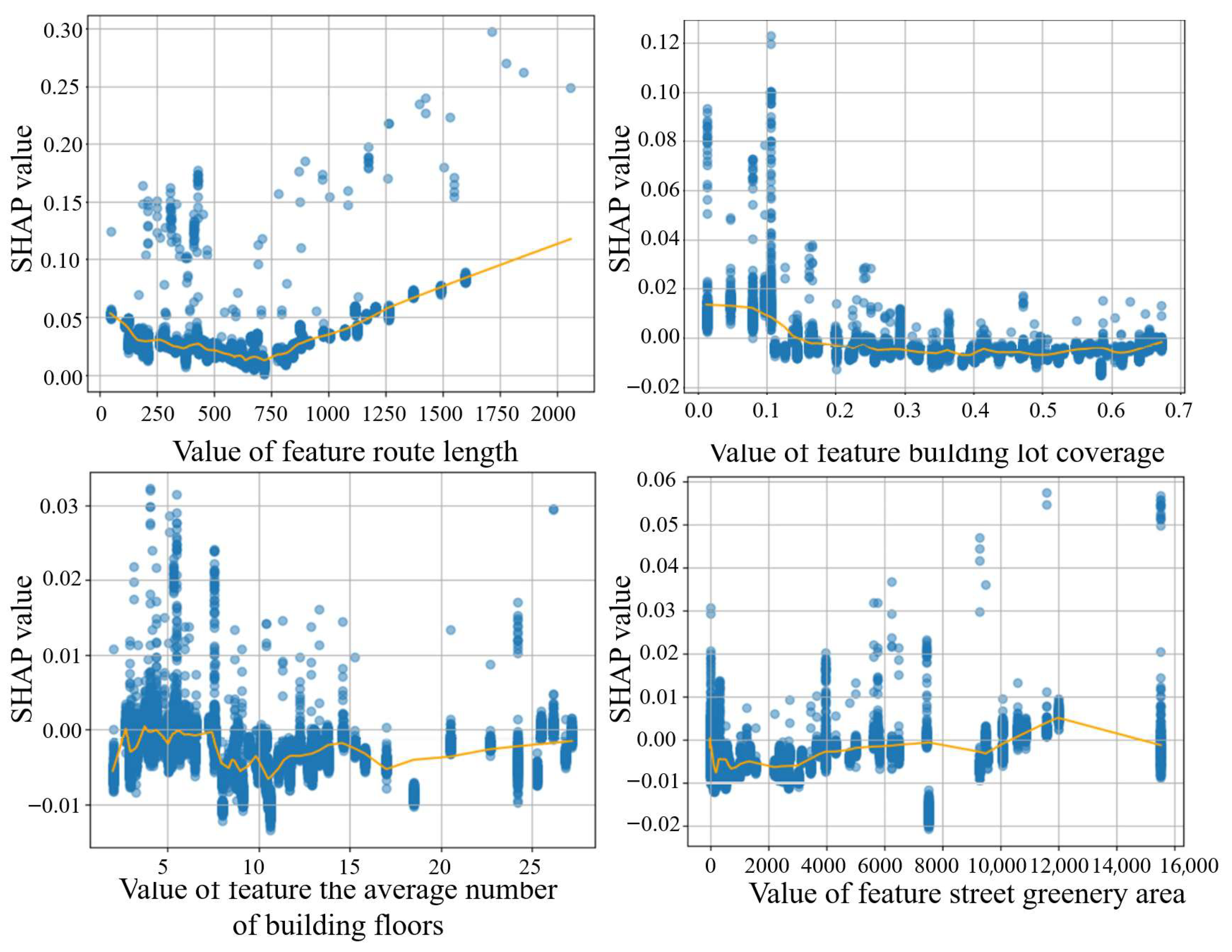
Each plot (Figure 3 and Figure 4) has an x-axis representing the built environment variable and a y-axis representing the variables’ impact on destination choice. The relationship between non-commuters’ destination choices and the length of their routes is explored in Figure 3, which illustrates a nonlinear correlation. Initially, predictions made by the model display some variability and uncertainty. For shorter routes, the trend of the SHAP value (a measure used in the model) starts at 0.05 and declines until it reaches a minimum of 750 m. Within this range, the influence of route length on destination choice appears irregular, with SHAP values varying significantly. However, a notable shift occurs as the route length extends beyond 750 m. It indicates that for routes shorter than 750 m, non-commuters tend to choose the shorter option, aligning with general travel behavior studies. However, when the route exceeds 750 m, the presence of key attractions along the way might lead them to opt for a longer route. This nonlinear effect could be due to threshold effects, interactions with other variables, or varying sensitivities to route length at different scales.
Figure 3 presents an interesting pattern in how building lot coverage influences visitors’ destination choices. It reveals a negative correlation between destination choice and building lot coverage. However, the scenario changes when the building lot coverage exceeds 0.15. Beyond this point, the local effect exhibits unstable fluctuations. This instability suggests that the impact of building lot coverage on destination choice becomes marginal and less predictable as it increases beyond 0.15. Essentially, this data indicates a clear preference among visitors for routes where building lot coverage is 0.15 or less, implying an aversion to areas with higher building density.
The results in Figure 3 indicate that for building floors between two and seven, SHAP values remain steady around zero, suggesting minimal impact on destination choice. This stability likely reflects those shorter buildings, often older with fewer amenities or attractions, which are less appealing to travelers. For buildings taller than seven floors, SHAP values show oscillations with small peaks around 15 and 25 floors and dips at 11 and 17 floors, all within a narrow range of 0.01. These findings suggest nonlinear effects of building height on predictions, though these effects may be masked by data variability or other factors.
Figure 3 presents a pattern that can be observed concerning the impact of the amount of street greenery on visitor destination choices. The effect of street greenery on destination choice seems to have a nonlinear association that obtains stronger over time as more greenery is added. Initially, increasing green space shows a positive correlation with visitor preference, as moderate amounts of street trees, pocket parks, and linear greenways enhance the destination. However, this relationship reaches a critical threshold at approximately 12,000 m2, beyond which additional greenery yields declining marginal utility. This threshold phenomenon emerges because excessive consolidated green spaces, particularly large monofunctional parks, begin to compromise urban vibrancy. They reduce land available for complementary amenities, create inconvenient walking distances between destinations, and diminish the mixed-use character that attracts non-commuters seeking multipurpose visits.
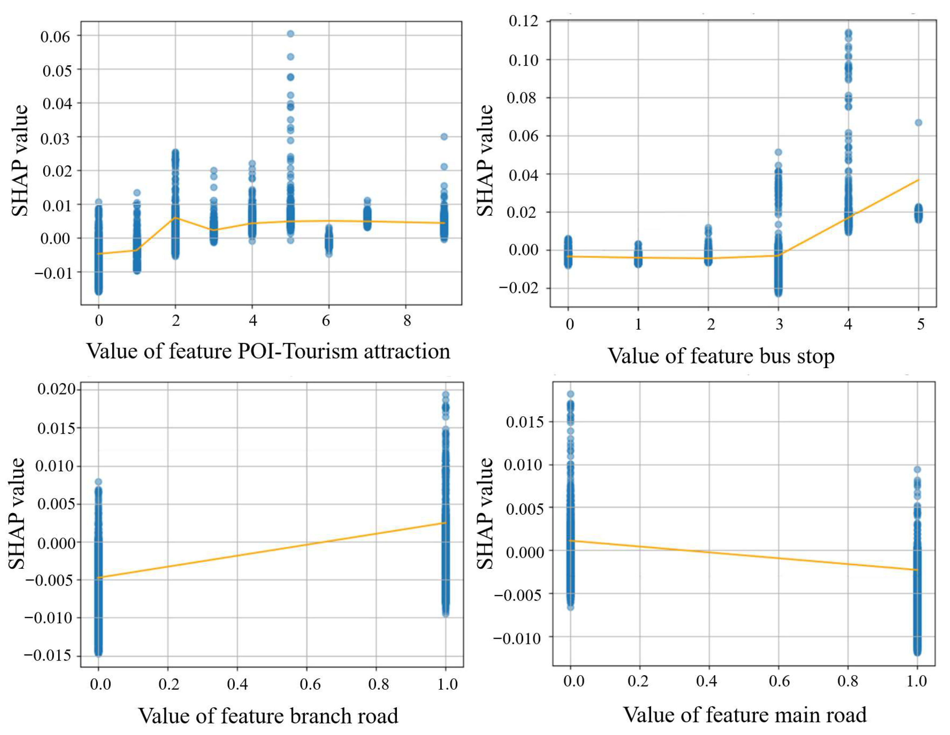
The dynamics of how non-commuters’ destination choice is influenced by the number of tourism attractions are illustrated in Figure 4. When there is a small number of tourism attractions together, the study shows a significant nonlinear relationship. More specifically, compared to more POIs, the SHAP value linked to a single POI-Tourism attraction is found to be lower. When there are more than two POI-Tourism attractions, the SHAP value increases. The link shown stabilizes with increased tourism attractions, indicating a saturation limit beyond which new attractions no longer have a meaningful increased marginal impact on destination choice. As the number of attractions increases, the emergent pattern shows that although the initial addition of attraction points significantly impacts destination preferences, this influence peaks, and the nonlinear effect either decreases or may disappear.
The nonlinear impacts of the POI-Bus stop on destination choice are shown in Figure 4. The empirical investigation of SHAP values concerning bus stops along a route demonstrates a consistent trend with minor variance when the count varies from zero to three stops. There are no nonlinear effects observed in this observation, and the effective magnitude is almost zero. In contrast, a noticeable change in perspective is observed when bus stops are increased to four, indicating the start of a strong nonlinear effect. In this case, the quantifiable SHAP value falls between 0.02 and 0.04. Nevertheless, it is essential to mention that the consequences of more than six bus stops are still unclear because there is not enough data given. This pattern points to a threshold effect on tourism whereby, as the number of bus stops on a certain route is above a critical figure, a significant increase in appeal is observed. Bus stops are usually placed in locations with high population density and infrastructure, which contributes to a synergistic impact in terms of accessibility and convenience. This helps explain part of the occurrence.
The analysis of SHAP values that correlate with the rest of the built environment variables, including POI-Museum, daily life facility, hotel, catering, shop, parking, entertainment, land use mix, and sidewalk width, shows that these values are marginally variable and do not show strong nonlinear relationships. Within the estimated results, a thorough discussion of these aspects is not possible due to the lack of a significant nonlinear association. The application of SHAP value analysis to the variables pertaining to road levels is restricted to the identification of positive or negative correlations; nonlinear dynamic relationships cannot be identified due to the binary coding representation of these variables, which is represented by the numbers 0 and 1. This is illustrated graphically in Figure 4. The element concerning main roads is found to have a negative association, but the factor concerning branched roads shows a positive correlation. This implies that non-commuters have a preference for minor roads.

6. Discussion and Conclusions

This study explored the nonlinear impact of the built environment on non-commuters’ destination choices in the catchment areas of metro stations, underscoring the role of metro railway systems in urban mobility. By applying a Random Forest model in conjunction with SHAP analysis, this study has revealed the relative significance of several factors in forecasting non-commuters’ destination choices. The SHAP analysis indicates that, even with the presence of tourism-related attractions, people’s preferences for destinations are more influenced by environmental factors, particularly parameters related to the location’s physical layout and accessibility.
The results show that “route length” is the most influential element in non-commuters’ destination choices, which is consistent with the literature [53,54]. While it is commonly understood that pedestrians generally prefer the shortest possible routes, this study found that beyond a threshold of 750 m, some respondents tend to choose longer routes that may offer greater experiential value.
Key factors such as building lot coverage, the average number of building floors, street greenery area, and the presence of POI like tourism attractions and bus stops significantly influenced destination choices. While existing literature demonstrates travelers’ preference for dense urban environments [55,56,57], it typically quantifies the built environment through land use diversity rather than specific structural variables such as “building lot coverage” and “average number of building floors,” which more directly capture building characteristics beyond mere land use. The existence of variables like “bus stop” and “POI-Tourism attraction” supports the idea that accessibility and connection play a major role in influencing travelers’ preferences [55,57].
However, these influences exhibit variability and context-dependent effects. Thus, apart from route length, which has been extensively demonstrated to have a significant impact on travel behavior, other variables show context-dependent effects, suggesting that non-commuters make complicated and nuanced decisions [2,55]. It is clear from the negative impact of “level of roads-main roads” on destination choice relative to the positive effect of “level of roads-branch roads” that people prefer the comfort and attractiveness of smaller streets over bigger ones [58].
The social-demographic parameters “age,” “gender-female,” and “concerns about crowdedness” are indicative of a variety of non-commuter profiles and the complex nature of travel experiences, even though these variables have less impact on destination choice. More social demographic variables, psychological, and cultural dimensions (e.g., perceived safety, esthetic preferences) warrant investigation through complementary qualitative approaches.
The study demonstrated the nonlinear relationships between various built environment factors around metro stations and non-commuters’ destination choices. The impact of these factors was found to vary significantly depending on the scale and context, indicating a need for nuanced urban planning approaches. Prior research on the travel behavior of non-commuters used the walkability score, which includes built environment factors (such as distance\the block length\the intersection density) for the general population, but no clear association was discovered [59]. Thus, walkability and transportation choice assessments tailored to urban non-commute travel are needed.
As a result, this study contributes to the field by identifying the aspects of the built environment that non-commuters find most significant. These findings contribute to the broader discourse on sustainable urban travel, emphasizing the role of efficient and attractive public transportation systems in urban non-commuters’ destination choices. The study underscores the importance of considering the built environment’s functional and esthetic aspects in shaping non-commuter experiences and choices. This analysis can benefit urban planners and businesses looking to optimize location choices or transport authorities aiming to improve the appeal and accessibility of certain areas around metro stations.
The findings yield concrete recommendations for optimizing metro station areas to serve non-commuters. Planners should implement a dual-path pedestrian network: shorter direct routes (<750 m) with efficient wayfinding for utilitarian trips, complemented by longer experiential paths (800–1200 m) along branch roads enriched with street greenery (>20% visibility) and amenity clusters. To enhance walkability, main roads require pedestrian-priority interventions like widened sidewalks, while branch roads should integrate placemaking elements. Building densities should target four–six floors with 60–70% lot coverage to balance vibrancy and comfort. High-attraction destinations like tourist sites and transit stops must be positioned within 400 m of station exits with clear visual connections. These evidence-based strategies, derived from our SHAP analysis of route length thresholds and built environment interactions, offer measurable benchmarks for TOD implementation. A phased approach is advised, beginning with pilot corridors in select station areas before scaling successful interventions, ensuring designs align with the nonlinear behavioral patterns our study reveals.
While this study has identified key built environment factors influencing non-commuters’ destination choices, several important limitations suggest directions for future research. First, our analysis did not incorporate socio-economic variables such as income levels and educational attainment, which may interact with built environment features to shape travel preferences. For instance, higher-income individuals might prioritize different amenities or tolerate longer walking distances than lower-income groups. Second, individual travel histories and habitual patterns, potentially significant moderators of destination choice, were not captured in our dataset. Future studies could employ longitudinal tracking methods to account for these behavioral nuances. Third, weekend sampling ensured focus on non-commuting trips; future research could compare weekday/weekend patterns to assess temporal variations in destination choices. For instance, weekday non-commuters might prioritize convenience-oriented amenities (e.g., pharmacies) over leisure destinations. Future research should expand to examine diverse metro station typologies, including urban centers, suburban nodes, and transitional urban zones.

Author Contributions

Conceptualization, Y.L.; methodology, Y.L. and H.D.; software, Y.L.; formal analysis, Y.L. and H.D.; investigation, Y.L.; writing—original draft preparation, Y.L. and H.D.; writing—editing, Y.L. and H.D.; visualization, Y.L. and H.D.; supervision, Y.L. and H.D.; project administration, Y.L. and H.D.; funding acquisition, Y.L. All authors have read and agreed to the published version of the manuscript.

Funding

This research was funded by the National Natural Science Foundation of China, grant number 5240080218.

Data Availability Statement

The data that support the findings of this study are available from the corresponding author, Hua Du, upon reasonable request.

Conflicts of Interest

The authors declare no conflicts of interest.

References

  1. Pryor, E.G. Parallel development of strategic land-use and transport planning: The case of the Territorial Development Strategy. In Land-Use/Transport Planning in Hong Kong: A Review of Principles and Practices; Harry, T., Dimitriou, A.H.S.C., Eds.; Routledg: London, UK, 1998. [Google Scholar]
  2. Dill, J.; McNeil, N. Transit and Active Transportation Use for Non-Commute Travel Among Portland Transit-Oriented Development Residents. Transp. Res. Rec. 2023, 2677, 151–168. [Google Scholar] [CrossRef]
  3. Liu, K.; Qiu, P.; Gao, S.; Lu, F.; Jiang, J.; Yin, L. Investigating urban metro stations as cognitive places in cities using points of interest. Cities 2020, 97, 102561. [Google Scholar] [CrossRef]
  4. Chen, T.; Hui, E.C.; Wu, J.; Lang, W.; Li, X. Identifying urban spatial structure and urban vibrancy in highly dense cities using georeferenced social media data. Habitat Int. 2019, 89, 102005. [Google Scholar] [CrossRef]
  5. Allis, T.; Fraga, C. Tourism, public transport and sustainable mobility. Transp. Rev. 2018, 38, 681–683. [Google Scholar] [CrossRef]
  6. Research Report on the Operational Characteristics of Green Transportation in Chengdu; Chengdu-Institute-of-Planning&Design: Chengdu, China, 2022.
  7. Beijing’s Metro Handles over 10 Million Weekday Passengers; Beijing-Municipal-Commission-of-Transport: Beijing, China, 2023.
  8. Yang, J.; Chen, J.; Le, X.; Zhang, Q. Density-oriented versus development-oriented transit investment: Decoding metro station location selection in Shenzhen. Transp. Policy 2016, 51, 93–102. [Google Scholar] [CrossRef]
  9. Wang, C.; Wang, X.; Pan, R.; Yan, Y. Influence of built environment on subway trip origin and destination: Insights based on mobile positioning data. Transp. Res. Rec. 2022, 2676, 693–710. [Google Scholar] [CrossRef]
  10. Tilahun, N.; Thakuriah, P.V.; Li, M.; Keita, Y. Transit use and the work commute: Analyzing the role of last mile issues. J. Transp. Geogr. 2016, 54, 359–368. [Google Scholar] [CrossRef]
  11. Xiao, L.; Lo, S.; Liu, J.; Zhou, J.; Li, Q. Nonlinear and synergistic effects of TOD on urban vibrancy: Applying local explanations for gradient boosting decision tree. Sustain. Cities Soc. 2021, 72, 103063. [Google Scholar] [CrossRef]
  12. An, D.; Tong, X.; Liu, K.; Chan, E.H. Understanding the impact of built environment on metro ridership using open source in Shanghai. Cities 2019, 93, 177–187. [Google Scholar] [CrossRef]
  13. Vale, D.S.; Pereira, M.; Viana, C.M. Different destination, different commuting pattern? Analyzing the influence of the campus location on commuting. J. Transp. Land Use 2018, 11, 1–18. [Google Scholar] [CrossRef]
  14. Sun, B.; Ermagun, A.; Dan, B. Built environmental impacts on commuting mode choice and distance: Evidence from Shanghai. Transp. Res. Part D Transp. Environ. 2017, 52, 441–453. [Google Scholar] [CrossRef]
  15. Singh, U.; Upadhyay, S.P.; Jha, I. The co-production of space in a tourist city: A case of Dharamshala. Cities 2022, 131, 103998. [Google Scholar] [CrossRef]
  16. Hall, C.M.; Le-Klähn, D.-T.; Ram, Y. Tourism, Public Transport and Sustainable Mobility; Channel View Publications: Bristol, UK, 2017; Volume 4. [Google Scholar]
  17. Ibraeva, A.; Correia, G.H.d.A.; Silva, C.; Antunes, A.P. Transit-oriented development: A review of research achievements and challenges. Transp. Res. Part A Policy Pract. 2020, 132, 110–130. [Google Scholar] [CrossRef]
  18. Jamme, H.T.; Rodriguez, J.; Bahl, D.; Banerjee, T. A Twenty-Five-Year Biography of the TOD Concept: From Design to Policy, Planning, and Implementation. J. Plan. Educ. Res. 2019, 39, 409–428. [Google Scholar] [CrossRef]
  19. Niu, S.F.; Hu, A.; Shen, Z.W.; Lau, S.S.Y.; Gan, X.Y. Study on land use characteristics of rail transit TOD sites in new towns-taking Singapore as an example. J. Asian Archit. Build. Eng. 2019, 18, 19–30. [Google Scholar] [CrossRef]
  20. Basaran, G.G.; Ingvardson, J.B.; Nielsen, O.A. Does transit-oriented development (TOD) influence perceived safety and mode choice? J. Transp. Land Use 2025, 18, 237–267. [Google Scholar] [CrossRef]
  21. Shao, R.; Derudder, B.; Yang, Y.; Witlox, F. The association between transit accessibility and space-time flexibility of shopping travel: On the moderating role of ICT use. J. Transp. Geogr. 2023, 111, 103661. [Google Scholar] [CrossRef]
  22. Gan, Z.; Yang, M.; Feng, T.; Timmermans, H.J. Examining the relationship between built environment and metro ridership at station-to-station level. Transp. Res. Part D Transp. Environ. 2020, 82, 102332. [Google Scholar] [CrossRef]
  23. Papa, E.; Bertolini, L. Accessibility and Transit-Oriented Development in European metropolitan areas. J. Transp. Geogr. 2015, 47, 70–83. [Google Scholar] [CrossRef]
  24. Berawi, M.A.; Saroji, G.; Iskandar, F.A.; Ibrahim, B.E.; Miraj, P.; Sari, M. Optimizing Land Use Allocation of Transit-Oriented Development (TOD) to Generate Maximum Ridership. Sustainability 2020, 12, 3798. [Google Scholar] [CrossRef]
  25. Gan, Z.; Feng, T.; Wu, Y.; Yang, M.; Timmermans, H. Station-based average travel distance and its relationship with urban form and land use: An analysis of smart card data in Nanjing City, China. Transp. Policy 2019, 79, 137–154. [Google Scholar] [CrossRef]
  26. Yong, J.; Zheng, L.J.; Mao, X.W.; Tang, X.; Gao, A.; Liu, W.N. Mining metro commuting mobility patterns using massive smart card data. Phys. A Stat. Mech. Its Appl. 2021, 584, 126351. [Google Scholar] [CrossRef]
  27. Tian, P.; Cai, M.; Wu, H.; Wang, J.J.; Liu, L.B.; Yang, H.; Peng, Z.H. Unraveling the accessibility-usage mismatch: Identifying driving factors and weather-sensitive metro stations using GPS data for improved metro competitiveness. Cities 2025, 159, 105794. [Google Scholar] [CrossRef]
  28. Edrisi, A.; Lahoorpoor, B.; Lovreglio, R. Simulating metro station evacuation using three agent-based exit choice models. Case Stud. Transp. Policy 2021, 9, 1261–1272. [Google Scholar] [CrossRef]
  29. Gronau, W. Encouraging behavioural change towards sustainable tourism: A German approach to free public transport for tourists. J. Sustain. Tour. 2017, 25, 265–275. [Google Scholar] [CrossRef]
  30. Zamparini, L.; Domenech, A.; Miravet, D.; Gutierrez, A. Green mobility at home, green mobility at tourism destinations: A cross-country study of transport modal choices of educated young adults. J. Transp. Geogr. 2022, 103, 103412. [Google Scholar] [CrossRef]
  31. Masiero, L.; Hrankai, R. Modeling tourist accessibility to peripheral attractions. Ann. Tour. Res. 2022, 92, 103343. [Google Scholar] [CrossRef]
  32. Liu, H.B.; Li, X.; Cardenas, D.A.; Yang, Y. Perceived cultural distance and international destination choice: The role of destination familiarity, geographic distance, and cultural motivation. J. Destin. Mark. Manag. 2018, 9, 300–309. [Google Scholar] [CrossRef]
  33. Alvarez, E.; Brida, J.G. An agent-based model of tourism destinations choice. Int. J. Tour. Res. 2019, 21, 145–155. [Google Scholar] [CrossRef]
  34. Cavallaro, F.; Galati, O.I.; Nocera, S. A tool to support transport decision making in tourist coastal areas. Case Stud. Transp. Policy 2019, 7, 540–553. [Google Scholar] [CrossRef]
  35. Li, P.; Yang, Q.; Lu, W.; Xi, S.; Wang, H. An Improved Machine Learning Framework Considering Spatiotemporal Heterogeneity for Analyzing the Relationship Between Subway Station-Level Passenger Flow Resilience and Land Use-Related Built Environment. Land 2024, 13, 1887. [Google Scholar] [CrossRef]
  36. Li, P.K.; Chen, X.M.; Lu, W.B.; Wang, H.; Yu, L. Built Environment’s Non-Linear Impact on Subway Passenger Flow Through Improved Interpretable Machine Learning. Transp. Res. Rec. 2025, 2679, 44–66. [Google Scholar] [CrossRef]
  37. Ramakrishnan, G.A.; Roy, P.; Varshney, H.K.; Srinivasan, K.K. A Joint Metro Train Demand Model Accounting for Disaggregate Consideration Probability and Aggregate Footfall. Appl. Sci. 2025, 15, 5216. [Google Scholar] [CrossRef]
  38. Tao, T.; Wu, X.; Cao, J.; Fan, Y.; Das, K.; Ramaswami, A. Exploring the nonlinear relationship between the built environment and active travel in the twin cities. J. Plan. Educ. Res. 2023, 43, 637–652. [Google Scholar] [CrossRef]
  39. Tu, M.; Li, W.; Orfila, O.; Li, Y.; Gruyer, D. Exploring nonlinear effects of the built environment on ridesplitting: Evidence from Chengdu. Transp. Res. Part D Transp. Environ. 2021, 93, 102776. [Google Scholar] [CrossRef]
  40. Yang, L.; Ao, Y.; Ke, J.; Lu, Y.; Liang, Y. To walk or not to walk? Examining non-linear effects of streetscape greenery on walking propensity of older adults. J. Transp. Geogr. 2021, 94, 103099. [Google Scholar] [CrossRef]
  41. Abdollahpour, S.S.; Buehler, R.; Le, H.T.K.; Hankey, S. Data aggregation impacts on built environment-mode share models around public transit stations. J. Transp. Land Use 2025, 18, 397–424. [Google Scholar] [CrossRef]
  42. Xu, T.; Zhang, M. Tailoring empirical empirical research on transit access premiums for planning applications. Transp. Policy 2016, 51, 49–60. [Google Scholar] [CrossRef]
  43. Chengdu-Daily. Traffic Statistics of Kuanzhaixiangzi Alleys. Available online: http://www.cdrb.com.cn/epaper/cdrbpc/202301/29/c109942.html (accessed on 29 January 2023).
  44. Sichuan Provincial Department of Culture and Tourism. Ticket Revenue Statistics of A-Class Scenic Spots in Chengdu; Sichuan Provincial Department of Culture and Tourism: Chengdu, China, 2021. Available online: https://wlt.sc.gov.cn/scwlt/hydt/2021/4/7/5fd14f25898d42d0ac7017bbe148c6e7.shtml (accessed on 7 April 2021).
  45. Jan Gehl, B.S. How to Study Public Life; Island Press: Washington, DC, USA, 2013. [Google Scholar]
  46. Tang, B.-s.; Wong, S.W.; Ho, W.K.; Wong, K.T. Urban land uses within walking catchment of metro stations in a transit-oriented city. J. Hous. Built Environ. 2020, 35, 1303–1319. [Google Scholar] [CrossRef]
  47. Lau, S.S.Y.; Giridharan, R.; Ganesan, S. Multiple and intensive land use: Case studies in Hong Kong. Habitat Int. 2005, 29, 527–546. [Google Scholar] [CrossRef]
  48. Prasad, A.M.; Iverson, L.R.; Liaw, A. Newer classification and regression tree techniques: Bagging and random forests for ecological prediction. Ecosystems 2006, 9, 181–199. [Google Scholar] [CrossRef]
  49. Cheng, L.; Chen, X.; De Vos, J.; Lai, X.; Witlox, F. Applying a random forest method approach to model travel mode choice behavior. Travel. Behav. Soc. 2019, 14, 1–10. [Google Scholar] [CrossRef]
  50. Chuang, L.-Y.; Yang, C.-H.; Li, J.-C.; Yang, C.-H. A hybrid BPSO-CGA approach for gene selection and classification of microarray data. J. Comput. Biol. 2012, 19, 68–82. [Google Scholar] [CrossRef]
  51. Lundberg, S.M.; Lee, S.-I. A unified approach to interpreting model predictions. Adv. Neural Inf. Process. Syst. 2017, 30, 4768–4777. Available online: https://dl.acm.org/doi/10.5555/3295222.3295230 (accessed on 4 December 2017).
  52. Bovy, P.H. On modelling route choice sets in transportation networks: A synthesis. Transp. Rev. 2009, 29, 43–68. [Google Scholar] [CrossRef]
  53. Lue, G.; Miller, E.J. Estimating a Toronto pedestrian route choice model using smartphone GPS data. Travel. Behav. Soc. 2019, 14, 34–42. [Google Scholar] [CrossRef]
  54. Sevtsuk, A.; Basu, R.; Li, X.; Kalvo, R. A big data approach to understanding pedestrian route choice preferences: Evidence from San Francisco. Travel. Behav. Soc. 2021, 25, 41–51. [Google Scholar] [CrossRef]
  55. Huang, A.; Levinson, D. Axis of travel: Modeling non-work destination choice with GPS data. Transp. Res. Part C Emerg. Technol. 2015, 58, 208–223. [Google Scholar] [CrossRef]
  56. Fang, J. Exploring the Role of the Built Environment in Studying Mode Choice Using a Tour-Based Approach. Ph.D. Dissertation, University of Florida, Gainesville, FL, USA, 2022. Available online: https://ufdcimages.uflib.ufl.edu/UF/E0/05/86/35/00001/Fang_J.pdf (accessed on 15 April 2022).
  57. Kheyrabadi, S.A.; Mamdoohi, A.R. The Influence of Origin Attributes on the Destination Choice of Discretionary Home-Based Walk Trips. ISPRS Int. J. Geo-Inf. 2024, 13, 218. [Google Scholar] [CrossRef]
  58. Tang, L.; Huang, Z.; Su, H. Evaluation of street walkability considering green view index. J. Hum. Settl. West China 2025, 40, 58–64. [Google Scholar]
  59. Hall, C.M.; Ram, Y. Measuring the relationship between tourism and walkability? Walk Score and English tourist attractions. J. Sustain. Tour. 2019, 27, 223–240. [Google Scholar] [CrossRef]
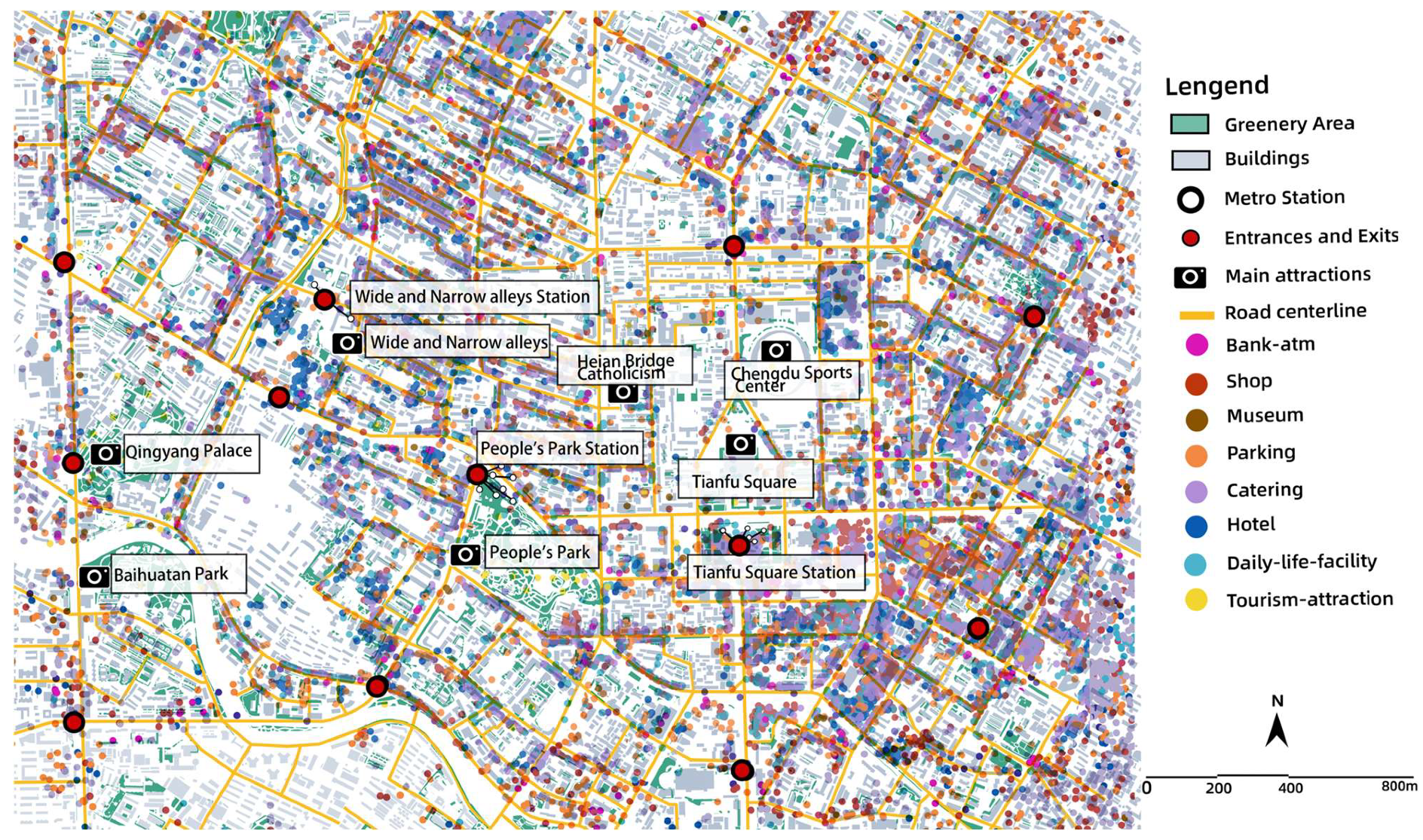
Figure 1. The study area.
Land 14 01619 g001
Figure 2. SHAP values of independent variables and SHAP explanations.
Land 14 01619 g002
Figure 3. The SHAP value plot (1).
Land 14 01619 g003
Figure 4. The SHAP value plot (2).
Land 14 01619 g004
Table 1. Sample characteristics.
CategoriesNumber (Percentage)
Age9 to 18 years111 (12.7%)
19 to 49 years641 (73.6%)
50 to 76 years119 (13.7%)
GenderFemale526 (60.4%)
Male345 (39.6%)
Frequency of visits to the adjacent area (times per year)Less than 1 time (including 1)498 (57.2%)
2 to 10 times84 (9.6%)
More than 10 times289 (33.2%)
Concerned levels of crowdedness when selecting a destinationVery concerned82 (9.4%)
Somewhat concerned324 (37.2%)
Normal211 (24.2%)
Not really concerned220 (25.3%)
Unconcerned34 (3.9%)
Table 2. Built environment variables.
VariablesDescriptionLevels and Units at the Street Level of the Destination
Sidewalk widthThe weighted average sidewalk width along the trip’s route on both sides.A continuous number in meters.
Street greenery areaThe greening shadow, grasslands, etc., along the trip’s route on both sides.A continuous number in m2.
The average number of building floorsIt equals the total building area of all floors of all buildings divided by the total floor area along a road.A continuous number.
Building lot coverageDivide the total building front length on either side of the road by the total length of the route.A ratio between 0 and 2.
Levels of roadsTwo levels: Main road and branch road 1, 0
Route lengthThe total length of the trip route.A continuous number in meters.
Land use mixA combination of land use categories is determined by the total floor area of the buildings on both sides of the travel route.A continuous number between 0 and 1.
The number of bus stopsBus stops are located along the route of the trip. Two stops owning the same name on either side of the road link in opposite directions count as one stop.A continuous number.
The number of each type of POIAccounting for the total number of each of the nine types shown in Table 3.A continuous number.
Table 3. Descriptive statistics of the built environment attributes at the street level of the destination.
AttributesMaxMinStandard DeviationMean
Sidewalk width (m)21.90.102.676.6
Street greenery area (m2)15,54704889.983855.64
The average number of building floors27.184.0212.979.30
Building lot coverage0.670.010.180.26
Route length (m)2061.8147.70335.81486.98
Land use mix0.800.350.080.66
The number of bus stops501.651.49
POI:
  Catering63016.5720.80
  Tourism attraction901.961.60
  Hotel2306.986.24
  Bank—atm200.420.11
  Museum501.381.09
  Shop3107.519.87
  Parking1402.964.02
  Daily life-facility3105.9611.02
  Entertainment1904.214.09
Levels of roads—main roads10--
Levels of roads—branch roads10--
Table 4. The distribution of route length.
Route Length (Meters)The Number of Samples
More than 160010
1200 to 140045
800 to 1200109
400 to 800475
Less than 400504
Disclaimer/Publisher’s Note: The statements, opinions and data contained in all publications are solely those of the individual author(s) and contributor(s) and not of MDPI and/or the editor(s). MDPI and/or the editor(s) disclaim responsibility for any injury to people or property resulting from any ideas, methods, instructions or products referred to in the content.