Urban Subway Station Site Selection Prediction Based on Clustered Demand and Interpretable Machine Learning Models

Abstract

With accelerating urbanization, the development of rail transit systems—particularly subways—has become a key strategy for alleviating urban traffic congestion. However, existing studies on subway station site selection often lack a spatially continuous evaluation of site suitability across the entire study area. This may lead to a disconnect between planning and actual demand, resulting in issues such as “overbuilt infrastructure” or the “island effect.” To address this issue, this study selects Kunming City, China, as the study area, employs the K-means++ algorithm to cluster existing subway stations based on passenger flow, integrates multi-source spatial data, applies a random forest algorithm for optimal positive sample selection and driving factor identification, and subsequently uses a LightGBM-SHAP explainable machine learning framework to develop a predictive model for station location based on mathematical modeling. The main findings of the study are as follows: (1) Using the random forest model, 20 key drivers influencing site selection were identified. SHAP analysis revealed that the top five contributing factors were connectivity, nighttime lighting, road network density, transportation service, and residence density. Among these, transportation-related factors accounted for three out of five and emerged as the primary determinants of subway station site selection. (2) The site selection prediction model exhibited strong performance, achieving an R² value of 0.95 on the test set and an average R² of 0.79 during spatial 5-fold cross-validation, indicating high model reliability. The spatial distribution of predicted suitability indicated that the core urban area within the Second Ring Road exhibited the highest suitability, with suitability gradually declining toward the periphery. High-suitability areas outside the Third Ring Road in suburban regions were primarily aligned along existing subway lines. (3) The cumulative predicted probability within a 300 m buffer zone around each station was positively correlated with passenger flow levels. Overlaying the predicted results with current station locations revealed strong spatial consistency, indicating that the model outputs closely align with the actual spatial layout and passenger usage intensity of existing stations. These findings provide valuable decision-making support for optimizing subway station layouts and planning future transportation infrastructure, offering both theoretical and practical significance for data-driven site selection.

1. Introduction

Rapid urbanization has intensified the imbalance between transportation supply and demand, resulting in worsening traffic congestion and environmental degradation. Against this backdrop, urban rail transit has emerged as a cornerstone of sustainable urban development due to its energy efficiency, coordination, and operational effectiveness [1]. It plays a vital role in enhancing public transport efficiency, alleviating congestion, optimizing land use, and improving the urban living environment [2,3]. Among these, rail transit stations function as key transportation hubs supporting the daily commuting needs of a large segment of the urban population [4] and play a pivotal role in high-density urban planning [5]. The areas surrounding these stations often become focal points of development, accessibility, and mixed-use activities, fostering vibrant, diverse, and dynamic urban environments. These areas attract various human activities and generate synergistic effects such as economic growth and job concentration [6,7]. Therefore, the planning and design of subway stations and their surrounding areas directly influence travel behavior, quality of life, and the sustainability of urban development. However, the current process of urban rail transit station site selection still faces several challenges. On the one hand, station layouts often fail to align with the spatial distribution of urban functional zones, limiting their ability to meet primary travel demands. On the other hand, certain station locations neglect integration with other transportation modes, resulting in pronounced “last-mile” problems. Furthermore, site selection decisions frequently rely on experiential judgment rather than comprehensive multi-factor analysis and scientific evaluation. This often leads to inadequate service coverage and low operational efficiency, thereby failing to effectively relieve traffic congestion or guide the orderly development of urban space. Therefore, it is imperative to develop a more scientific and systematic methodology for station site selection that enables the integrated optimization of transport efficiency and urban spatial functionality.

The selection of rail transit station locations represents a critical component of transportation planning. A well-planned site selection can enhance the attractiveness of public transportation, promote balanced urban development, and strengthen the overall functionality and vitality of the city [8]. In response to the challenges associated with site selection, recent studies have increasingly integrated multi-source data and intelligent algorithms to improve the scientific rigor and practical effectiveness of the selection process. The origins of site selection research in the field of transportation date back to the 1950s, when scholars began exploring mathematical approaches to evaluate the placement and layout of major transit stations [9]. With advances in computer and information technologies, research on rail transit site selection has evolved from relying solely on traditional qualitative methods to the widespread adoption of advanced techniques such as spatial analysis, data mining, and model optimization [10]. For instance, the use of geographic information systems (GIS) and remote sensing technologies has improved the accuracy of urban transportation data acquisition and processing, thereby enhancing decision-making support [11]. Additionally, the incorporation of methods such as transportation demand forecasting, traffic assignment models, and operations research-based optimization techniques [12,13] has made site selection for rail transit more scientific and accurate [14]. In recent years, research on rail transit site selection has adopted a multi-dimensional analytical approach, considering factors such as environmental protection, economic returns, and social impacts [15]. Some scholars have also proposed a site selection framework rooted in the principles of sustainable development, emphasizing the importance of holistically considering the interrelationship between rail transit, the urban environment, and the economy. This approach aims to improve the attractiveness of subway travel [16,17] and maximize passenger volume [18].

As research on site selection continues to deepen, the emergence of multi-source geospatial data has become a key resource for addressing site selection challenges. When integrated with machine learning techniques, such data can significantly enhance prediction accuracy and facilitate complex decision-making processes [19,20]. A growing number of researchers are employing multi-source spatial data as input to develop predictive models using machine learning algorithms for site selection studies. For instance, Niu et al. [21] used subway stations in Lanzhou City, China, as the research subject, and developed a site selection prediction model based on 19 spatial indicators using the random forest algorithm. They validated the model’s performance through K-fold cross-validation and a 300 m buffer zone overlap analysis, ultimately achieving an AUC score of 0.9823. Amini et al. [22] proposed a hybrid algorithm that integrates artificial neural networks (ANNs) with network optimization for site and hub selection in the Chengdu subway network. El Ozadi et al. [23] introduced a hybrid algorithm that incorporates machine learning for the strategic site selection of urban shared transportation hubs (e.g., metro-logistics integration points), facilitating the coordinated optimization of rapid transit and freight logistics. Amini et al. [24] integrated the “node-place” model with machine learning approaches to classify rail transit stations, assessing their efficiency to inform subsequent site selection and development intensity evaluations. Although previous studies have effectively demonstrated the practicality of machine learning algorithms in transportation-related site selection and achieved promising results, they have largely simplified the site selection problem into a binary classification task—determining whether a particular area “should have a station”—while overlooking the continuous gradient of spatial suitability across different locations. Moreover, in terms of factor selection, current studies often lack the integration of multi-source data. Regarding training sample selection, most studies do not assess the quality of existing stations and instead treat all of them as positive samples for model training. However, not all existing stations represent high-quality site selections with optimal locations. This undifferentiated sampling approach may introduce noise, compromise the model’s ability to identify key site selection factors, and reduce the scientific rigor and practical validity of the predictions. Research has shown that rail transit site selection must comprehensively consider various factors, including existing transportation infrastructure, population density, urban functional zoning, land use, and levels of economic development [25]. Machine learning can efficiently process large volumes of multi-source data, accurately predict demand, simulate alternative scenarios, and identify key factors to optimize site selection strategies—thereby enhancing the accuracy and efficiency of decision making. Moreover, these methods are flexible and adaptable to diverse urban environments.

According to data from the China Urban Rail Transit Association, by the end of 2024, 58 cities in mainland China had operational urban rail transit systems, comprising 361 lines with a total operating mileage of 12,160.77 km. Among them, subway lines accounted for 9306.09 km, representing 76.53% of the total mileage. Subway stations serve as critical nodes within urban rail transit systems, and their spatial distribution directly influences urban structure, transport efficiency, and the rational allocation of resources. With accelerating global urbanization, residents in high-density cities are becoming increasingly reliant on subway stations [26]. To address the limitations of existing research on urban rail transit station site selection, this study integrates explainable machine learning models with data-driven approaches, incorporating multi-source spatial factors—such as urban spatial structure, functional facilities, socio-economic conditions, and natural environment—to systematically analyze the key determinants and spatial suitability of subway station locations. Specifically, this study employs cluster analysis to identify the functional attributes and usage patterns of various types of subway stations within urban spaces, thereby supporting the selection of positive samples for location prediction models. In terms of model performance, compared with existing studies, cluster-based positive sample selection improves the R² value from 0.48 to 0.89 and reduces the MSE from 0.104 to 0.024. The selected positive samples are then used with a random forest algorithm to identify key influencing features, which are subsequently input into the LightGBM (Light Gradient Boosting Machine) model to map the spatial suitability distribution of subway stations across the urban area. Model accuracy and the suitability of existing subway station sites are evaluated through spatial overlay analysis with current stations and assessment of actual passenger flow data. This study provides a quantitative basis for scientifically selecting subway station locations. It also offers theoretical support, practical strategies, and novel insights for urban planning departments to optimize rail transit layouts, improve urban accessibility, and promote sustainable development amid multi-objective trade-offs.

2. Study Area and Data

2.1. Study Area

The selected study area, Kunming, is a key economic, cultural, and transportation hub in southwest China. In recent years, Kunming has experienced rapid urban development. To address the transportation pressures associated with urbanization, Kunming Metro has constructed multiple lines since 2011 (Figure 1), covering the city’s core areas and major transportation nodes. As of now, the Kunming Metro network includes six operational lines, with a total length of 165.85 km and 103 stations, including 10 transfer stations. Since Kunming Metro Lines 1 and 2 are currently operated as a single integrated line, they are jointly referred to as “Line 1&2” in this study. Kunming is considered an emerging model city for subway development. Although subway construction in Kunming began relatively late, it has progressed rapidly. The Kunming Metro network remains under active planning, and research on station site selection prediction in this context holds exploratory significance. Therefore, this study focuses on the Kunming Metro as a research case to explore the spatial suitability of existing station locations and to predict the probability of future planned sites.

2.2. Data Description

The primary datasets used in this study, along with their sources, are summarized in

Table 1. Data used and sources.

Data	Data Sources
Metro station and line data	Kunming Institute of Surveying and Mapping
Road network and bus stop data	Kunming Institute of Surveying and Mapping
Building data	Building height of Asia in 3D-GloBFP (https://zenodo.org/records/12674244, accessed on 12 July 2025)
POI data	Amap (https://lbs.amap.com/, accessed on 12 July 2025)
Population density	Open Spatial Demographic Data and Research (http://www.worldpop.org, accessed on 12 July 2025)
Nighttime light	luojia1-01 (http://59.175.109.173:8888/app/login.html, accessed on 12 July 2025)
Digital Elevation Model (DEM)	Geospatial Data Cloud (https://www.gscloud.cn/, accessed on 12 July 2025)
Slope	Geospatial Data Cloud(https://www.gscloud.cn/, accessed on 12 July 2025)
Aspect	Geospatial Data Cloud (https://www.gscloud.cn/, accessed on 12 July 2025)
Landsat 8–9 satellite imagery	EarthExplorer (https://earthexplorer.usgs.gov/, accessed on 12 July 2025)

. Since the study area is divided into 100 m × 100 m grid cells for feature matrix construction, spatial resolution was a key criterion in data selection to ensure consistency with the analytical scale. Specifically, the resolution details of selected datasets are as follows: population density (100 m), nighttime light intensity (130 m), digital elevation model (DEM), slope, and aspect (30 m), and Landsat 8–9 satellite imagery (30 m).

3. Methods and Models

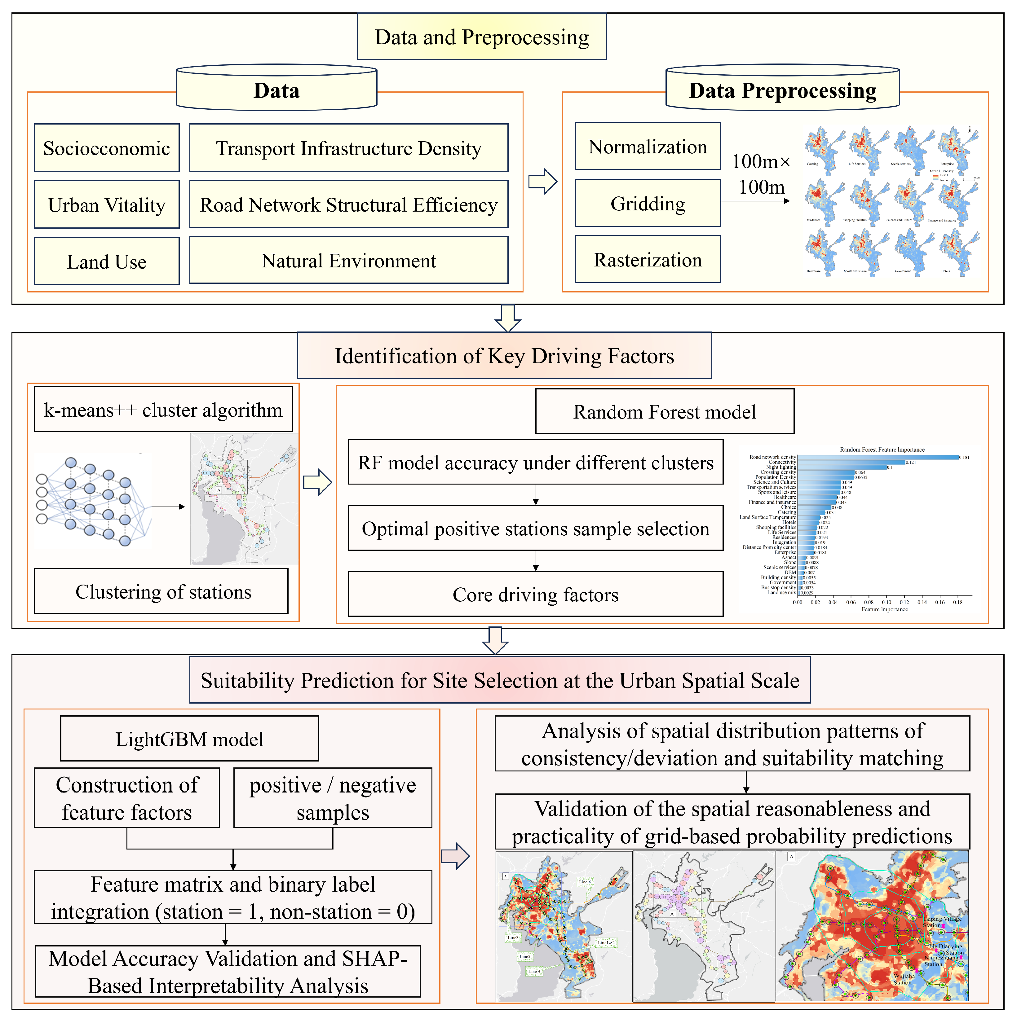
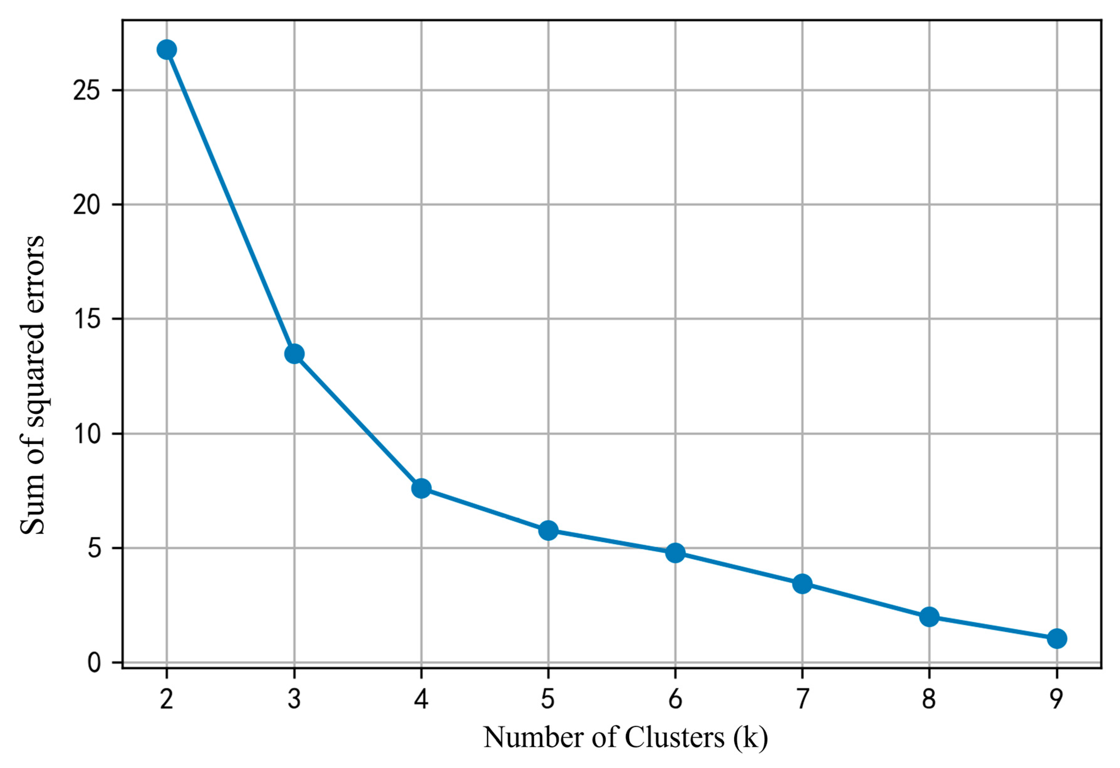
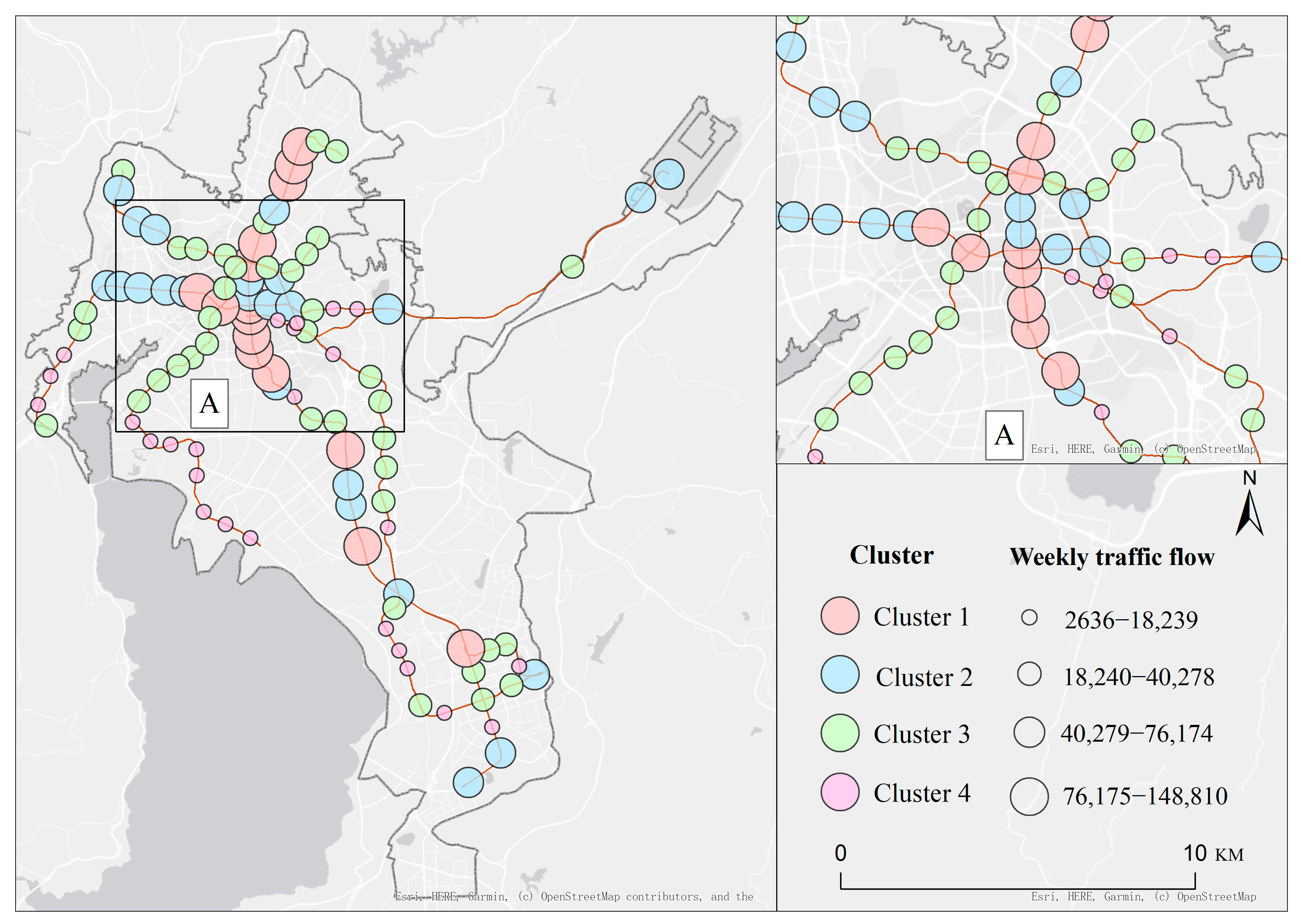
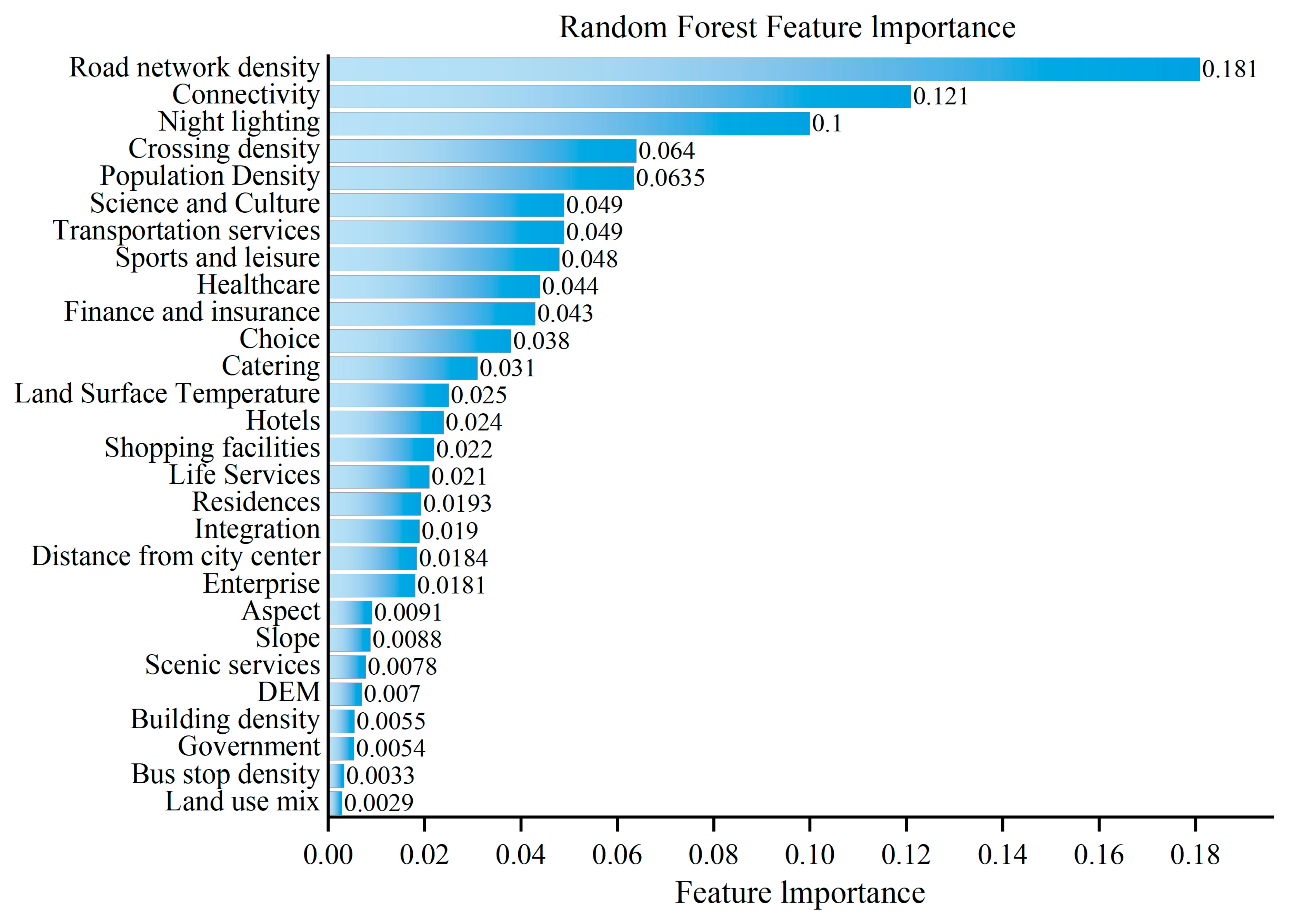
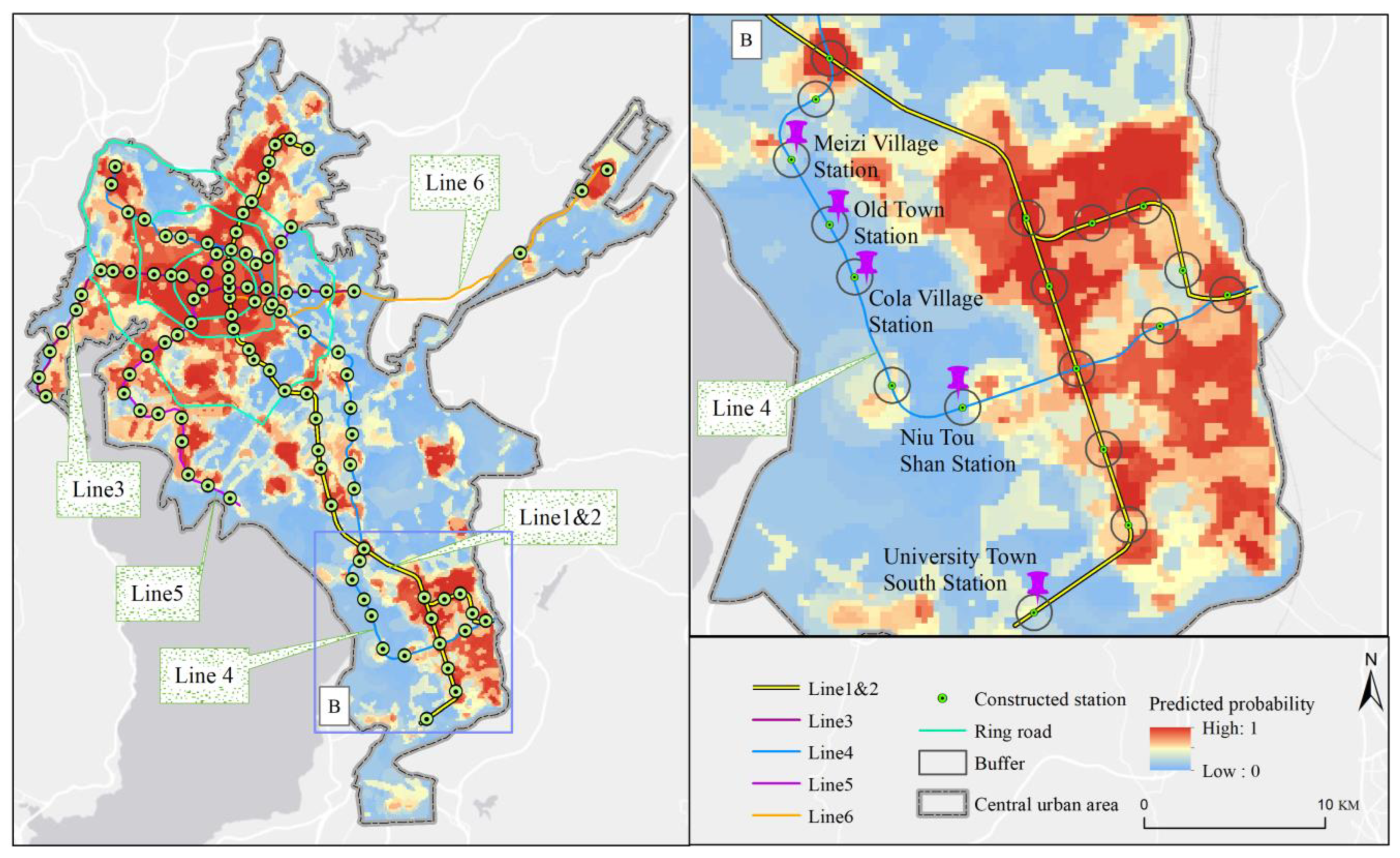
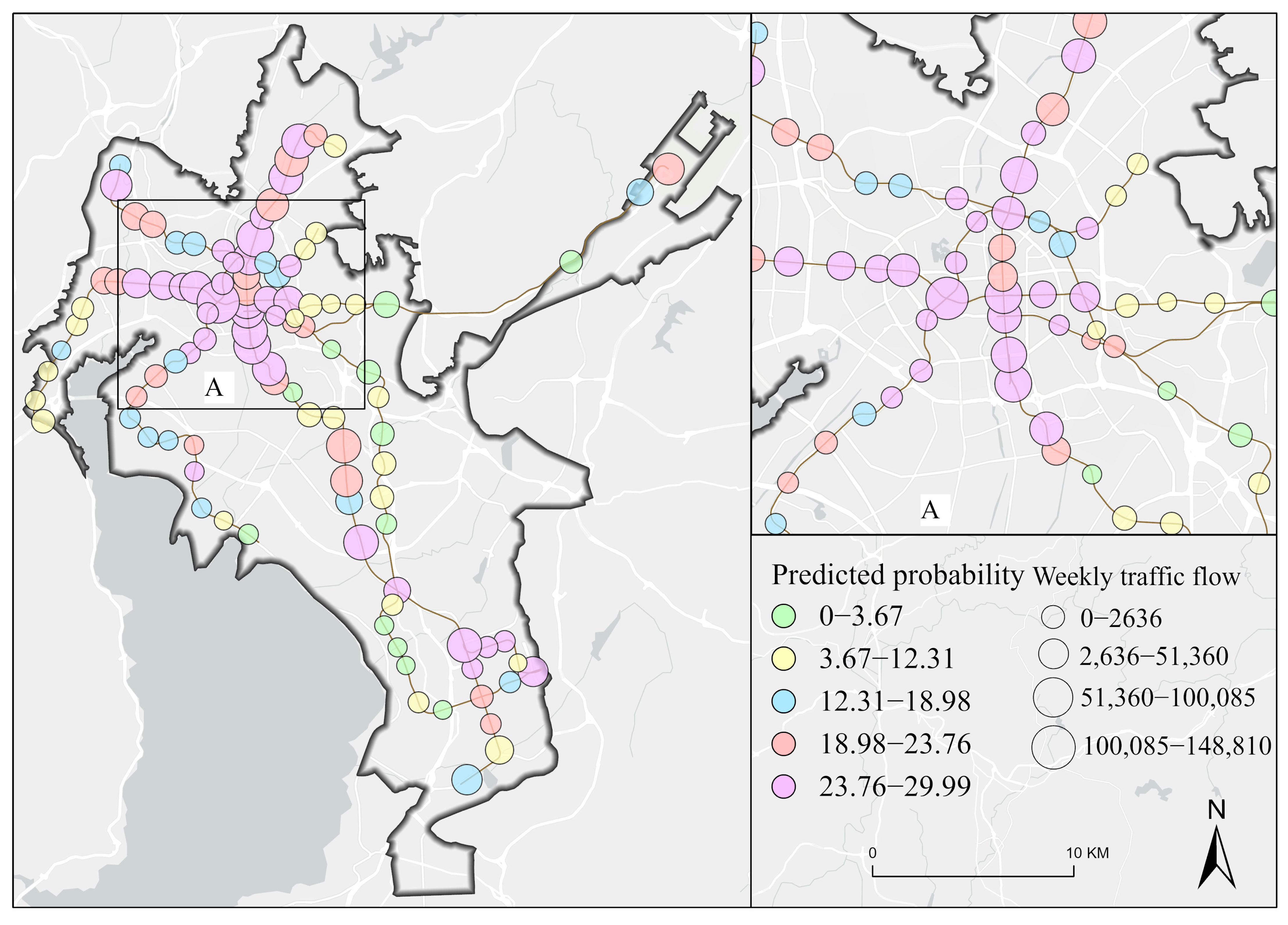
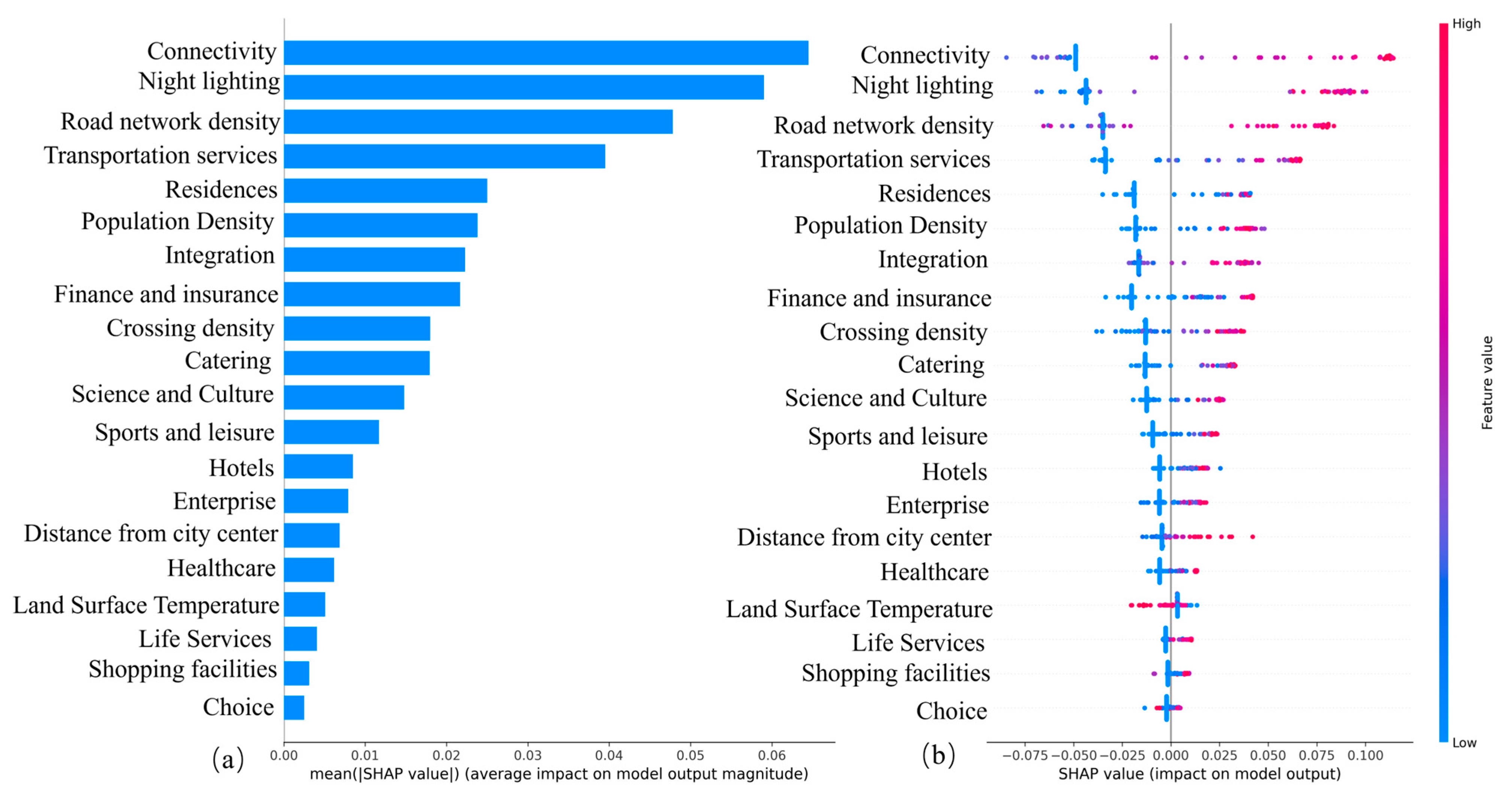
This study integrates spatial feature extraction, cluster analysis, machine learning modeling, and interpretive analysis to develop a mathematical modeling framework for predicting subway station locations. First, 28 spatial variables—such as nighttime light intensity, population density, and road network structure—are extracted to construct a gridded feature matrix. Cluster analysis is then conducted using passenger flow data from existing stations to extract optimal positive samples. Second, the optimal positive samples are combined with a random forest model to identify key site selection drivers. Variables with a feature contribution below 1% are excluded, resulting in a refined set of 20 features. These variables are then input into a LightGBM model for regression analysis, and SHAP values are used to interpret feature contributions, revealing how key factors influence site selection suitability. Finally, spatial predictions and visualizations of site suitability are generated at the city scale, providing scientific support and a quantitative decision-making basis for subway station planning. The technical workflow of this study is illustrated in Figure 2.

3.1. Selection of Influencing Factors for Rail Transit Station Location

This study primarily selects key factors influencing rail transit station site selection across the following dimensions: socio-economic conditions, urban vitality, land use, transportation infrastructure density, regional road network efficiency, and natural environment. The selection of these factors is informed by a synthesis of existing indicator systems in relevant literature, which serves as the foundation for constructing the feature matrix. This approach allows for the flexible construction of indicators based on specific research needs, which need not replicate original indicators as long as they comply with relevant standards [27]. Therefore, this study uses the existing indicator systems as a reference framework for constructing the feature system. Furthermore, this study does not pursue an extensive number of indicators but instead emphasizes that each essential factor influencing site selection is represented by at least one measurable indicator. The specific factors corresponding to each dimension are presented in

Table 2. Driving factors for site selection.

Dimension	Feature Factors
Socioeconomic [28,29]	Catering
	Life services
	Scenic services
	Enterprise
	Shopping facilities
	Financial and insurance services
	Science and cultural services
	Residences
	Sports and leisure
	Healthcare
	Government
	Hotels
Urban vitality [30,31]	Population density
	Nighttime light intensity
Land use [32,33]	Land use mix
	Building density
Transportation facility supply density (LST) [34]	Bus stop density
	Distance to city center
	Road network density
	Crossing density
	Transport services
Efficiency of regional road network structure [35]	Choice
	Connectivity
	Integration
Natural environment [36]	DEM
	Slope
	Aspect
	Land surface temperature

, along with the respective references for each.

(1)

Socioeconomic

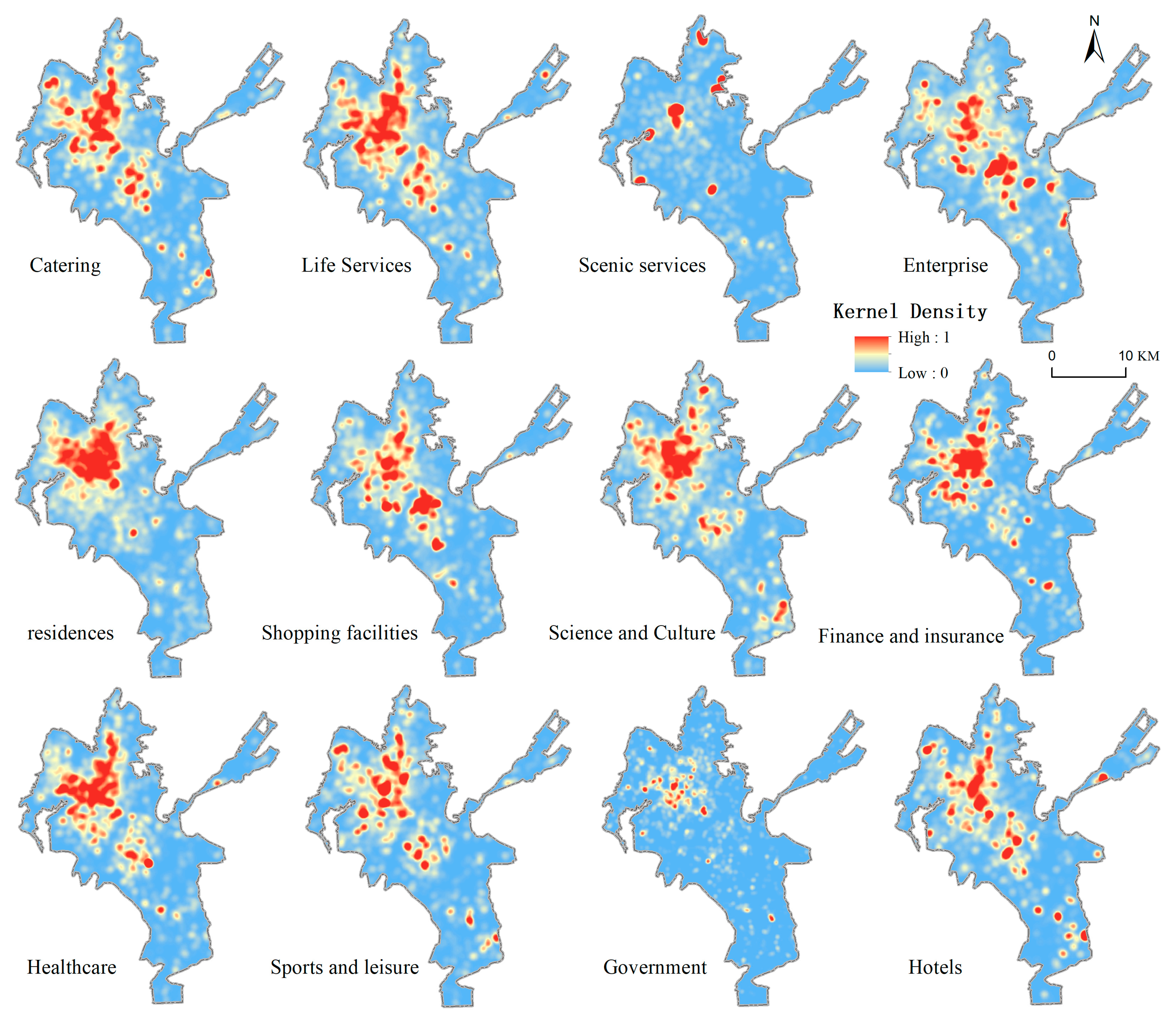
Data for the socioeconomic dimension were obtained by extracting POI information via the Amap API. Based on Amap’s classification standards [37], the POI data were categorized into 12 types, including the density of catering services, daily life services, and scenic spot services, resulting in 12 indicators representing the socioeconomic dimension (Figure 3).

(2)

Urban vitality

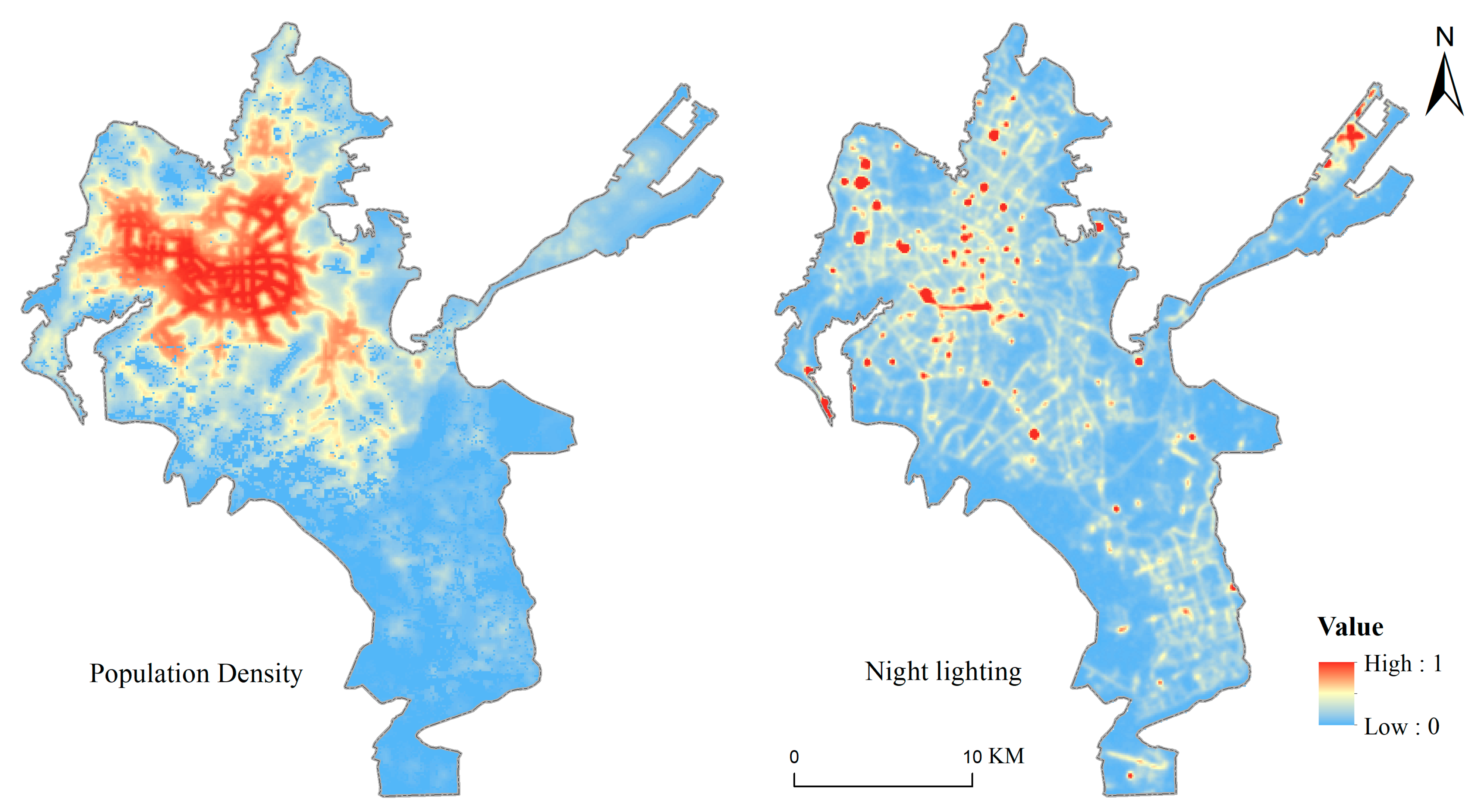
Urban vitality reflects the intensity of human activity and social interaction. In previous studies, nighttime light data and population density have been widely adopted as proxies for measuring urban vitality. Accordingly, this study adopts these two indicators as feature variables representing urban vitality (Figure 4).

(3)

Land use

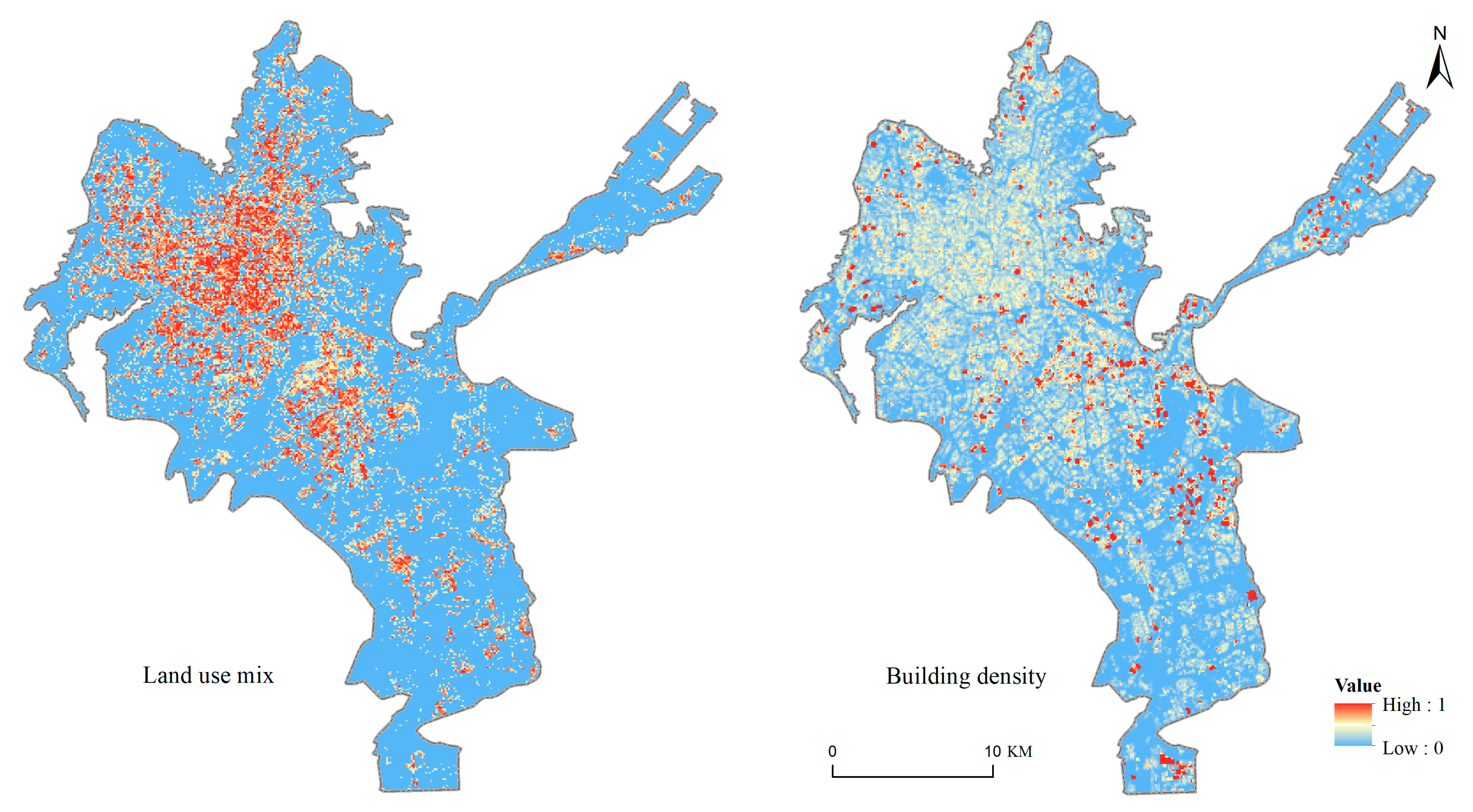
The land use dimension primarily includes two indicators: land use mix and building density (Figure 5). Specifically, land use mix is calculated based on the distribution of POI types, with its computation defined in Formula (1). Building density is defined as the ratio of the total floor area of all buildings within a given grid cell to the total area of that cell, as shown in Formula (2).

$$L_{grid}=-{{\displaystyle {\displaystyle \sum }}}_{j=1}^s{a}_j\mathit{ln}{a}_j$$

(1)

where $L_{grid}$ denotes the land use mix within a specific grid cell, $s$ represents the total number of POI types in grid i, and $a_i$ denotes the proportion of POI type j relative to all POI types in the grid.

$$B_i={{\displaystyle {\displaystyle \sum }}}_{i=1}^n{A}_i/A_{grid}$$

(2)

where $A_i$ represents the area of the i-th building (in square meters, m²), n denotes the number of buildings within a specific grid cell, and $A_{grid}$ refers to the area of a single grid cell (in square meters, m²).

(4)

Transportation facility supply density

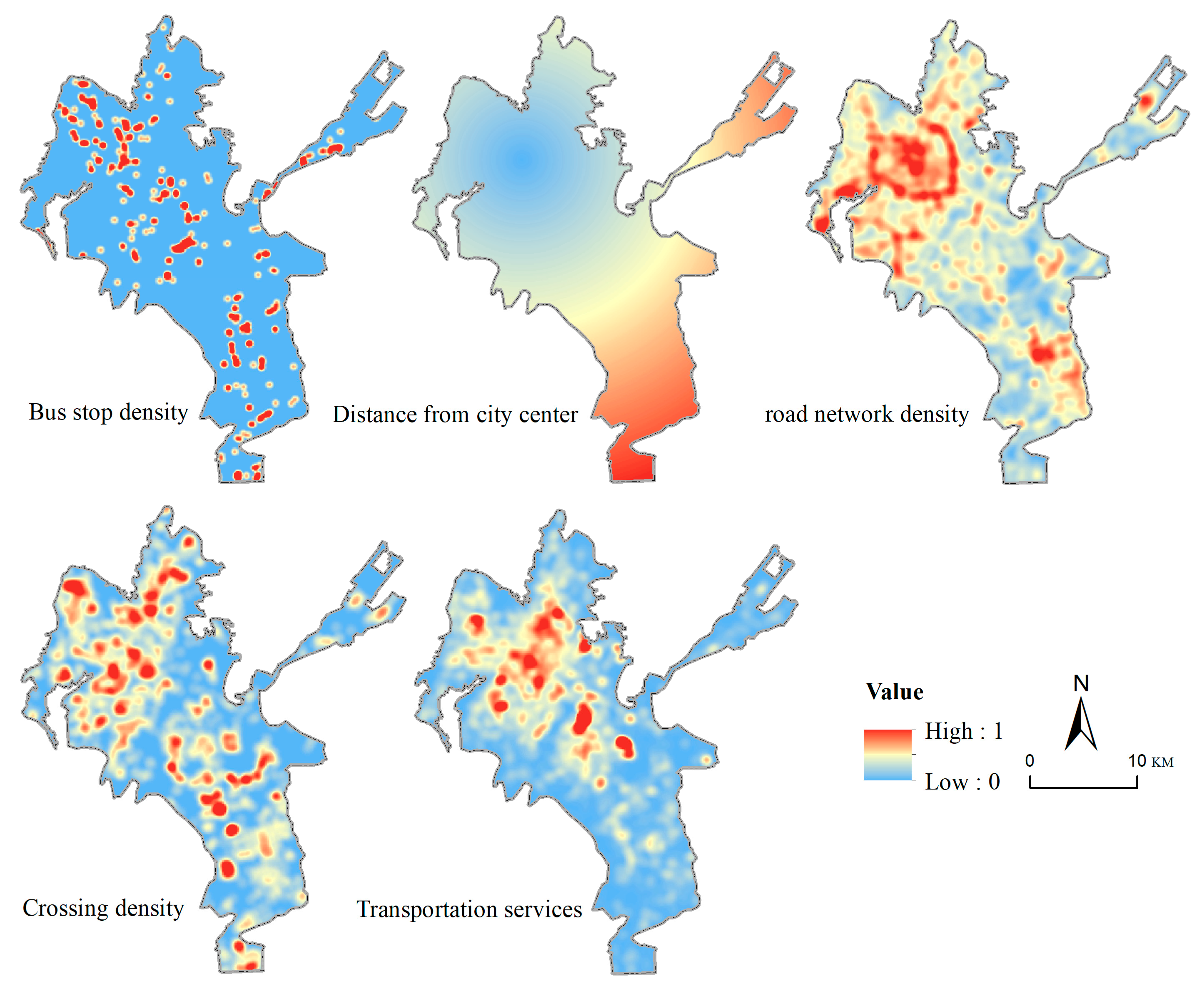
The transportation infrastructure supply density dimension characterizes the quantity, spatial distribution, and network coverage of transportation facilities surrounding each candidate site. It includes five indicators: intersection density, distance to the city center, bus stop density, road network density, and transportation service facility density (Figure 6). Among them, intersection density, distance to the city center, bus stop density, and road network density were calculated using spatial data provided by the Kunming City Surveying and Mapping Institute and processed in ArcGIS 10.8.1. In contrast, transportation service facility density was derived from Amap’s classification system and computed using kernel density estimation of POI data.

(5)

Efficiency of regional road network structure

The spatial efficiency of the regional road network was evaluated based on the topological efficiency of the road network, focusing on the spatial position of each candidate site within the urban road system and its influence on patterns and intensities of pedestrian flow, vehicle flow, visibility, and urban activities. The rail transit network was conceptualized as a graph consisting of stations (nodes) and connecting lines (edges), where each station corresponds to a node and the links between stations represent edges. Based on GIS data and spatial network theory, adjacency relationships between nodes are established. Indicators in this dimension are computed using Depthmap, based on space syntax theory and road network geometric data (line segments and nodes), and include three metrics: selectivity, connectivity, and integration (Figure 7). The corresponding calculation formulas are presented in Equations (3)–(5):

$$C_i={{\displaystyle {\displaystyle \sum }}}_{j\ne i}{{\displaystyle {\displaystyle \sum }}}_{k\ne i,j}{\displaystyle \frac{n_{ijk}}{n_{jk}}}$$

(3)

where $n_{ijk}$ is the number of shortest paths from node j to node k that pass through node i, and $n_{jk}$ denotes the total number of shortest paths between node j and node k.

$$M_i={{\displaystyle {\displaystyle \sum }}}_{j\in N_i}1$$

(4)

where $M_i$ represents the connectivity of node i, and $N_i$ denotes the set of nodes adjacent to node i.

$$I_i={\displaystyle \frac{N-1}{{\displaystyle \sum }_{i\ne j}{d}_{ij}}}$$

(5)

where $I_i$ represents the integration value of node i, N denotes the total number of nodes, and $d_{ij}$ is the distance between nodes i and j.

(6)

Natural environment

The selection of urban rail transit station locations in mountainous cities is characterized by distinct topographical adaptability. Kunming City, as a representative mountainous city, features highly undulating terrain and complex geological conditions, where natural environmental factors serve as fundamental constraints in station site selection. Accordingly, the natural environment dimension in this study primarily considers four key factors(Figure 8): Digital Elevation Model (DEM), slope gradient, slope aspect, and LST. LST was derived via the Google Earth Engine (GEE) platform using Kunming’s administrative boundary vector data and thermal infrared imagery (Band 10) from Landsat 9 through remote sensing inversion. The LST processing workflow involves cloud masking, emissivity correction, brightness temperature conversion, median synthesis of annual summer images (2022–2024), gap filling, and spatial clipping. This process ultimately produces a stable and reliable surface temperature distribution map, which is used to evaluate the influence of high-temperature zones on site comfort and the potential for pedestrian traffic aggregation.

In integrating multi-source spatial data, this study first standardized the coordinate systems of all vector and raster datasets to CGCS2000. Vector data (e.g., road networks, subway stations, and subway lines) underwent spatial topology checks and corrections based on three rules: no overlapping points, no dangling lines, and no gaps in polygon features. Topological errors were batch-identified using Check Geometry (ArcGIS) and shapely.validation.explain_validity (Python 3.7.1), followed by manual inspection. Raster datasets—including POI kernel density, nighttime light intensity, and population density—were resampled to a 100 m resolution.

As the datasets originated from different sources, their original spatial extents varied. To ensure consistency in model inputs, the smallest common bounding box across all layers was used as a reference. All datasets were uniformly cropped using NumPy 2.1.3slicing, with dimensions aligned by row and column count. Areas without data were uniformly assigned a value of 0 to eliminate the impact of NoData values on model training. Additionally, to ensure comparability across variables with differing units, all features were normalized using min–max scaling to a standardized range of [0, 1]. The final 28 input variables were stacked into a three-dimensional array of shape (434, 358, 28) and fed into the subsequent site selection prediction model.

3.2. K-Means++ Clustering

The K-means algorithm is a widely used clustering technique that begins by randomly selecting several initial centroid points [38,39]. It then calculates the distance between each data point and the centroids, assigning each point to the nearest cluster center [40]. However, the randomness in selecting initial centroids can significantly influence clustering outcomes, often leading to suboptimal results.

This study utilizes passenger flow data from subway stations to classify station types from a people-oriented perspective. Given that passenger flow data often exhibit multi-peak or multi-modal distributions and significant variability across stations, improper selection of initial centroids may result in inaccurate or unstable clustering outcomes. Therefore, K-means++ is adopted in this study as the clustering algorithm, as it strategically selects initial centroids that are relatively distant from one another, thereby reducing the influence of outliers on clustering performance [41]. This optimized initialization mechanism is better suited to the characteristics of passenger flow data.

After normalizing the data, the elbow method is applied to determine the optimal number of clusters, as illustrated in Figure 9. The slope of the SSE (sum of squared errors) curve shows a noticeable change at four clusters. Accordingly, four clusters are selected as the optimal number for classifying the passenger flow patterns of existing subway stations in the study area.

3.3. Feature Importance Calculation Based on Random Forest

The random forest model is an ensemble learning algorithm consisting of multiple decision trees. Due to its high spatial fitting accuracy, it has been widely applied to address multidimensional nonlinear problems [42]. In this study, the random forest model is primarily employed to compute feature importance—after normalization—using the Mean Decrease in Gini index (MDG), in order to identify the most influential variables affecting rail transit station site selection. The MDG value for feature importance is calculated as follows:

$${MDG}_r={\displaystyle \frac{{{\displaystyle \sum }}_{i=1}^n{{\displaystyle \sum }}_{j=1}^t{DG}_{rij}}{{{\displaystyle \sum }}_{r=1}^m{{\displaystyle \sum }}_{i=1}^n{{\displaystyle \sum }}_{j=1}^t{DG}_{rij}}}$$

(6)

where ${MDG}_r$ represents the importance of the r-th feature among all features; n is the number of decision trees; t is the number of nodes in a single tree; m represents the total number of features; and ${DG}_{rij}$ refers to the Gini impurity reduction contributed by the r-th feature at the j-th node of the i-th tree.

Based on their MDG values, all features are ranked in order of importance. A higher MDG value indicates a greater contribution to model performance. Generally, features with higher MDG values are considered the most influential factors in rail transit station site selection. Depending on the research objectives, the top k features with the highest MDG values are selected for further analysis.

3.4. LightGBM-Based Site Selection Prediction Model

To evaluate the performance advantages of LightGBM in site suitability regression, this study introduces four benchmark regression models—linear regression, ridge regression, random forest regression, and support vector regression—for comparative analysis. Model performance is assessed using root mean square error (RMSE), mean absolute error (MAE), and mean absolute percentage error (MAPE). All evaluation metrics were computed using spatial 5-fold cross-validation and are reported as mean ± standard deviation. The results indicate that LightGBM outperforms the other models across R², RMSE, and additional metrics (

Table 3. Comparison of model performance metrics.

Model	R2 (Mean ± SD, CV)	RMSE (Mean ± SD, CV)	MAE (Mean ± SD, CV)
Linear Regression	0.51 ± 0.0163	0.3456 ± 0.0194	0.2678 ± 0.0161
Ridge Regression	0.54 ± 0.0154	0.3391 ± 0.0187	0.2634 ± 0.0156
Random Forest	0.72 ± 0.0112	0.2134 ± 0.0145	0.1652 ± 0.0117
SVR	0.70 ± 0.0138	0.2678 ± 0.0162	0.2032 ± 0.0129
LightGBM	0.79 ± 0.0087	0.1654 ± 0.0123	0.1189 ± 0.0091

), demonstrating that its nonlinear modeling and feature interaction capabilities provide substantial advantages for addressing complex geospatial prediction tasks.

Therefore, this study adopts LightGBM regression as the primary modeling approach for predicting subway station site suitability. The model takes multi-source spatial features of grid cells as input and outputs a continuous suitability score for potential station locations. The objective is to learn the relationship between spatial features and the likelihood of a grid cell being suitable for a subway station. LightGBM is a highly efficient implementation of the gradient boosting decision tree framework. It uses a leaf-wise (leaf-first) growth strategy and an efficient histogram-based feature binning mechanism, which significantly improve large-scale data processing capacity and training speed while maintaining high accuracy [43,44]. The model is trained iteratively by minimizing the squared error loss function, gradually constructing and stacking multiple regression trees to approximate the true target values. The objective function is presented in Equation (7). In each iteration, the loss function is approximated and optimized using a second-order Taylor expansion (Equation (9)) to improve training efficiency and model stability. To mitigate potential spatial autocorrelation and information leakage in high-resolution grid data, this study applies spatial K-fold cross-validation to evaluate the generalization capability of the LightGBM-based site selection model, using GroupKFold (n = 5) and setting grid_size = 1000 m.

(1)

Overall objective function

$${\gamma }^{\left(t\right)}={\displaystyle \sum }_{i=1}^{n}l(y_i,{\widehat{y}}_i^{\left(t-1\right)}+f_t\left(x_i\right))+\tau (f_t)$$

(7)

where ${\gamma }^{\left(t\right)}$ denotes the total loss of the t-th tree; $y_i$ is the true label of the i-th sample; ${\widehat{y}}_i^{\left(t-1\right)}$ is the predicted value of the i-th sample after the (t − 1)-th iteration; $f_t\left(x_i\right)$ represents the prediction increment for the i-th sample from the t-th tree; l(⋅)is the loss function, such as the squared error l(y, $\widehat{y}$) = ${(y-\widehat{y})}^2$; and $\tau \left(f_t\right)$ is the regularization term used to control model complexity, typically defined in Equation (8).

(2)

Regularization term

$$\tau \left(f\right)=\mathsf{\alpha }\mathrm{T}+{\displaystyle \frac{1}{2}}\mathsf{\beta }{\displaystyle \sum }_{j=1}^T{w}_i^2$$

(8)

where $T$ denotes the number of leaf nodes in the tree; $w_j$ is the output weight of the j-th leaf; $\mathsf{\alpha } \mathrm{a}\mathrm{n}\mathrm{d} \mathsf{\beta }$ are regularization parameters.

(3)

Approximate optimization: second-order Taylor expansion

$${\gamma }^{\left(t\right)}\approx {\displaystyle \sum }_{i=1}^n\left[{g_{i}f}_t\left(x_i\right)+{\displaystyle \frac{1}{2}}{h}_i{f}_t^2\left(x_i\right)\right]+\tau (f_t)$$

(9)

where $g_i={\displaystyle \frac{\partial l(y_i,{\widehat{y}}_i)}{\partial {\widehat{y}}_i}}$ denotes the first-order derivative (gradient), and $h_i$ = ${\displaystyle \frac{{\partial }^{2}l(y_i,{\widehat{y}}_i)}{\partial {\widehat{y}}_i^2}}$ denotes the second-order derivative (Hessian).

(4)

Prediction output formula

After M iterations of training, the model’s prediction is given as follows:

$${\widehat{y}}_i={\displaystyle \sum }_{t=1}^M{f}_t\left(x_i\right)$$

(10)

where ${\widehat{y}}_i$ is the predicted value of the i-th sample, and $f_t\left(x_i\right)$ is the output of the t-th regression tree for input $x_i$.

3.5. Feature Contribution Interpretation Based on Shapley Additive Explanations

This study employs the Shapley Additive Explanations (SHAP) framework to interpret the contribution of each feature to the model’s output. SHAP is a unified approach for interpreting the output of machine learning models [45]. Within the SHAP framework, each input feature is treated as a “participant” in the prediction process. The importance of each feature is quantified by its SHAP value, which reflects its marginal contribution to the model’s prediction. For a given sample x, the SHAP value of feature j is computed using the following formula:

$${\partial }_j\left(val\right)={{\displaystyle \sum }}_{s\in \left\{x_1,\dots ,x_p\right\}\left\{x_j\right\}}{\displaystyle \frac{\left|s\right|!\left(p-\left|s\right|-1\right)!}{p^{!}}}(val\left(S\cup \left\{x_j\right\}\right)-val\left(s\right))$$

(11)

where ${\partial }_j\left(val\right)$ represents the SHAP value of feature j in a specific prediction model, denoted as $val$. Assuming that S is a subset of input features, $\left|s\right|$ represents the number of features in subset S, and p represents the total number of features in the prediction model, the global SHAP value of variable j is calculated as the sum of the absolute SHAP values of j for all features in the dataset.

4. Results

4.1. Clustering of Station Passenger Flows and Identification of Spatial Characteristics

To identify the functional characteristics and usage patterns of different types of subway stations within the urban space, this study employs passenger flow data from all existing stations and applies the K-means++ clustering algorithm for station classification. Clustering analysis enables the identification of station types that differ in commuting demand, service coverage, and spatial configuration, thereby providing a structural basis for selecting high-value candidate stations in subsequent site selection modeling. Specifically, considering the cyclical nature of human activity, the total weekly inbound and outbound passenger flow at each station are used as the clustering variable to reflect overall usage intensity across temporal dimensions. To ensure the stability and representativeness of the clustering outcomes, data standardization is applied, and the optimal number of clusters is determined to be four using the elbow method. The clustering results and corresponding spatial distribution of existing subway stations based on passenger flow are presented in Figure 10.

The cluster analysis results identified four distinct types of station locations. To reveal spatial attribute differences among clusters, the standardized mean scores of stations within each cluster were calculated across six dimensions: socioeconomics, urban vitality, land use, transportation infrastructure supply, regional road network structure, and total passenger flow. Since the natural environment dimension primarily influences the construction feasibility of future planned sites and has limited relevance to the spatial characteristics and built environment of existing stations, it was excluded as a core reference in the cluster-based site type classification. The distribution of key indicators across clusters for each dimension is illustrated in Figure 11, while

Table 4. Statistical analysis of mean values for different dimensional characteristics of each cluster.

Cluster	Socioeconomic	Urban Vitality	Land Use	Density of Transport Facility Supply	Regional Road Network Efficiency	Average Total Passenger Flow	Number of Stations
Cluster 1	0.24	0.38	0.18	0.23	0.48	105,771	15
Cluster 2	0.14	0.30	0.12	0.20	0.36	64,952	24
Cluster 3	0.10	0.24	0.13	0.20	0.35	28,137	39
Cluster 4	0.05	0.17	0.09	0.18	0.29	10,646	25

reports the average values of dimensional characteristics for each cluster type.

Based on the multidimensional spatial indicator statistics derived from the clustering results (Figure 10 and Figure 11, Table 4), each category of subway stations exhibits clearly differentiated spatial characteristics. Cluster 1 exhibits the highest overall scores, characterized by strong socioeconomic conditions, high urban vitality, functional diversity, and superior network structure. These stations typically serve as major comprehensive hubs located in urban cores or regional sub-centers. Cluster 2 shows the second-highest scores, featuring balanced performance in transportation and land use, and is typically located near medium-density residential areas. Cluster 3 presents similar but slightly lower values compared to Cluster 2, especially in terms of average weekly passenger volume. It mainly includes stations located in peripheral, commuter-oriented areas. Cluster 4, by contrast, comprises stations located in underdeveloped peripheral zones, characterized by low passenger volumes, weak spatial functionality, and limited development levels—reflecting both their marginal position and future development potential within the urban system.

This suggests that not all existing stations exhibit favorable spatial characteristics or strong passenger flow performance. When using existing stations to predict future site selection, it is recommended to select “high-quality subway station samples” that demonstrate stronger functional clustering and greater transportation attraction potential. Therefore, in the subsequent model training phase, the selection of positive samples for predicting subway station suitability should be guided by clustering results, in order to construct a training set that balances high-quality samples with structural representativeness—thus improving model accuracy and generalization capability.

4.2. Optimized Selection of Positive Samples and Identification of Key Driving Factors

To improve the accuracy and sample adaptability of the subway station location prediction model, this study employs a random forest regression model trained on various cluster combinations derived from the clustering results. The predictive performance of each combination is compared to identify the optimal positive sample set for model training. In parallel, feature importance evaluation is conducted to identify key drivers influencing subway station location selection.

The methodology is as follows: fifteen different cluster categories and their combinations are used as candidate positive samples, while negative samples are randomly selected from urban areas without stations or with low passenger flow, using a sampling ratio of 3:1. These are combined to construct the training dataset. Each dataset comprising both positive and negative samples is modeled using a random forest algorithm. The average prediction accuracy is then evaluated using both validation and cross-validation methods. Based on these results, the optimal cluster combinations are selected as the final positive sample set for model training. As an example, the model accuracy results for six cluster combinations are presented in

Table 5. Accuracy of RF models under partial clustering and combinations thereof.

Station Clustering Combinations	Test R2	Test MSE
Cluster 1	0.803	0.045
Cluster 2	0.548	0.067
Cluster 1 + Cluster 2	0.891	0.024
Cluster 1 + Cluster 3	0.725	0.065
Cluster 1 + Cluster 2 + Cluster 3	0.495	0.113
Cluster 1 + Cluster 2 + Cluster 3 + Cluster 4	0.483	0.104

.

An evaluation of the predictive performance of 15 cluster combinations in the random forest model reveals that the highest accuracy is achieved when Clusters 1 and 2 are used jointly as positive samples, indicating strong feature separability and structural stability. In contrast, using individual clusters or combinations including Clusters 2 and 3 results in decreased model generalization, suggesting that their spatial features are relatively ambiguous and less conducive to forming stable predictive patterns.

After determining the optimal positive sample combination (Clusters 1 and 2), a random forest model was trained using all spatial features to identify key drivers of subway station site selection, and the importance scores of all variables were extracted. The model input consisted of 28 variables spanning multiple dimensions, including socioeconomic factors, urban vitality, land use, and transportation infrastructure supply density. The output was a binary classification label indicating whether a subway station should be established. Feature importance was assessed based on the average contribution of each variable to model accuracy across all decision tree node splits. The results of feature importance analysis are presented in Figure 12. To enhance the interpretability and generalization capability of the model, this study conducts feature selection based on model performance during training and compares the prediction accuracy of the LightGBM model on the validation set through repeated 5-fold cross-validation. The results indicate that removing variables with feature importance below 1% leads to optimal prediction performance on the validation set, as measured by R², RMSE, and MAE. The corresponding results are summarized in

Table 6. Cross-validation performance of the LightGBM model under different feature importance thresholds.

Threshold (%)	Number of Features Retained	R2	RMSE	MAE
No filtering	28	0.631	0.211	0.136
0.5%	26	0.689	0.202	0.131
1%	20	0.79	0.165	0.119
2%	16	0.705	0.207	0.134
3%	12	0.612	0.229	0.142
4%	10	0.525	0.291	0.144
5%	5	0.390	0.375	0.162

.

Therefore, the feature importance threshold was set to 1.0%. Eight variables falling below this threshold—namely slope, aspect, scenic service facilities, DEM elevation, building density, government facility density, bus stop density, and land use mix—were removed. The exclusion criteria were informed by prior studies recommending the control of variable redundancy, and were further supported by natural breakpoints observed in the feature importance distribution, ensuring that the removed variables contributed minimally to the prediction outcome. The final 20 site selection drivers included road network density, connectivity, nighttime lighting, intersection density, population density, transportation services, education and culture, sports and leisure, healthcare, financial services, choice, food and beverage services, surface temperature, hotel accommodation, shopping services, daily life services, residential density, spatial integration, distance to city center, and business services. These variables collectively constitute the core input features for the subsequent subway station site selection prediction model, reflecting the combined effects of service provision, urban vitality, spatial accessibility, and structural characteristics within the urban environment.

4.3. Spatial Distribution of Predicted Suitability for Metro Station Siting

To further evaluate the combined effects of site selection drivers and map the spatial distribution of subway station suitability at the urban scale, this study developed a site selection prediction model based on the LightGBM algorithm, building upon the previously identified features. The model inputs consist of 20 normalized spatial features, including population density, transportation connectivity, and functional facility density, all represented on a 100 m × 100 m spatial grid. The positive samples comprise existing subway stations categorized as Cluster 1 and Cluster 2. Their feature values are extracted based on spatial coordinate matching. In addition, a random sample of grid points without stations—twice the size of the positive sample set—is selected to ensure class balance and spatial representativeness.

Model training was performed using the default parameter configuration of LightGBM, with the dataset split into 70% for training and 30% for testing. Model robustness was evaluated through 5-fold cross-validation. The results indicate that the model achieves strong predictive performance, with an R² of 0.93 on the training set, 0.95 on the test set, an average R² of 0.83 from standard 5-fold cross-validation, and an average R² of 0.79 from spatial 5-fold cross-validation. These results suggest that the model maintains robust generalization capability even under spatial independence constraints. The hyperparameter settings of the LightGBM model are provided in

Table 7. Hyperparameter settings for the LightGBM model.

Hyperparameter	Description	Value
num_leaves	Maximum number of leaves in each tree	31
learning_rate	Controls the contribution of each tree to the model	0.05
max_depth	Limits the depth of each tree	−1
n_estimators	Total number of trees to be trained	100

.

To further evaluate the suitability of existing subway station sites, a 300 m buffer zone was generated around each station and spatially overlaid with the predicted suitability results from this study. The results are illustrated in Figure 13, Figure 14 and Figure 15. As illustrated in Figure 13, all existing stations located within the Third Ring Road in the central urban area, as well as terminal stations beyond the Third Ring Road, fall within areas of high predicted suitability. The predicted suitability exhibits a radial pattern extending outward from the city center: highest within the Second Ring Road, gradually decreasing toward the Third Ring Road. Beyond the Third Ring Road, areas of high suitability generally follow the alignment of subway lines, indicating strong spatial consistency. However, several stations show relatively low predicted suitability within their respective 300 m buffer zones, including Wujiaba Station (Lines 1&2), Hedianyong and Niujiezhuang Stations (Line 4), and Taipingcun Station (Line 3).

In the southern part of the central urban area, the site suitability prediction results are illustrated in Figure 14. The existing stations in this area are part of the Line 1&2 and Line 4 subway corridors. As indicated by the prediction results, with the exception of University Town South Station, which is classified as medium-low suitability, the stations along Line 1&2 and their surrounding 300 m buffer zones are predominantly situated in high-suitability areas. In contrast, Line 4 stations in this area generally exhibit low suitability scores, including Meizicun, Gucheng, Kelecun, and Niutoushan Stations. These stations and their corresponding 300 m buffer zones also fall within low-suitability areas. Indeed, according to the overall prediction outcomes, these stations exhibit the weakest spatial consistency with the model results across the entire study area.

The predicted suitability results for the central urban area and the northwestern extension of Line 6 are presented in Figure 16. Line 6, part of the Airport Central Line, includes only four stations beyond the Third Ring Road. According to the prediction results, both Eastern Bus Station and Dabanqiao Station exhibit relatively low suitability scores. Lines 1&2 and Line 4 are two subway corridors that run north–south through the central area of Kunming. Among them, the suitability of existing Line 1&2 stations within the central area is lower than that of stations located in the southern section and within the Third Ring Road. Similarly, Line 4 stations in the same area—including Zhujia Village, Yangputou, Yuyuan Road, and Tami Stations—along with their 300 m buffer zones, are all classified as low suitability. Additionally, the terminal station of Line 5, Baofengcun Station, also shows relatively low spatial consistency with the predicted suitability results.

To further examine the relationship between existing subway stations and predicted suitability outcomes, this study calculated the cumulative predicted probability within a 300 m buffer zone around each station. These probabilities were classified into five levels using ArcGIS’s natural breaks method and subsequently compared with passenger flow data. A high cumulative predicted probability within a buffer zone indicates strong alignment between existing subway stations and the model’s predicted suitability. The statistical results of cumulative predicted probabilities are presented in Figure 16. Stations with lower cumulative predicted probabilities are consistent with the findings of the previous analysis. Furthermore, a comparison with classified passenger flow data reveals that stations with higher cumulative predicted probabilities generally correspond to higher levels of passenger traffic. Conversely, stations with lower cumulative predicted probabilities tend to exhibit lower passenger traffic. This spatial consistency validates the effectiveness and explanatory capacity of the site selection prediction model in reflecting the actual spatial layout and operational patterns of urban subway stations, aligning closely with existing planning logic and usage intensity. These results not only highlight the model’s ability to accurately identify high-potential station locations but also demonstrate its strong capacity to reverse-engineer the operational intensity of existing stations, indicating high practical adaptability and valuable implications for urban transit planning.

4.4. Global Feature Contributions of Siting Drivers and Model Interpretation

This study evaluates the global contribution of each feature by averaging its absolute SHAP value. Figure 17 displays the SHAP value distribution for 20 features in the LightGBM-based station location prediction model. As shown in Figure 17a, connectivity emerges as the most influential feature in predicting subway station locations, underscoring the critical role of transportation network integration in station performance. As the backbone of urban mobility, rail transit station layouts must ensure efficient integration with existing transportation networks. This includes not only seamless transfers with other transportation modes—such as buses and roads—but also the accessibility of surrounding road networks, enabling convenient station access and enhancing overall system efficiency. The second most important feature is the nighttime lighting index, which captures the influence of nighttime urban activity intensity on station demand. Areas with higher nighttime lighting values typically indicate more active economic, commercial, and entertainment functions, as well as greater population density. Such areas tend to generate substantial passenger demand, necessitating the provision of rail transit services to meet travel needs—particularly in cities with high nighttime mobility, where this feature has notable implications for station site selection. Among the top five features are three related to urban transportation—connectivity, road network density, and transportation service—further emphasizing that spatial structure and service provision within the transportation system are key drivers of station suitability. These findings not only reflect the strong spatial dependency between subway stations and the urban transportation system, but also confirm the critical role of multimodal integration in optimizing site selection. Additionally, other features—such as population density and various POI-related indicators—interact with one another to jointly shape the rational spatial layout of rail transit stations.

Figure 17b presents the SHAP summary beeswarm plot, which illustrates the distribution of SHAP values for each variable. Each point is colored according to the corresponding variable value (blue = low, red = high) and positioned along the horizontal axis based on its SHAP value, indicating its contribution to increasing or decreasing the predicted probability of site selection. For instance, variables such as connectivity, nighttime lighting, and population density exhibit red long tails on the right and blue long tails on the left, suggesting that higher values of these variables increase site selection probability, thus serving as positive drivers. In contrast, lower values of these variables at specific locations correspond to reduced predicted site suitability.

Meanwhile, the surface temperature variable demonstrates a distinct “negative long-tail” pattern, with high-temperature areas (red) generally associated with negative SHAP values, indicating an inhibitory effect on suitability prediction. Conversely, low-temperature areas (blue) exhibit positive SHAP values, although their overall influence is limited. This indicates that the surface thermal environment has emerged as a significant limiting factor in subway station layout within the current study area. In particular, in urban areas affected by pronounced heat island effects, excessively high surface temperatures may reduce travel comfort and decrease residents’ willingness to use public transit, thereby reducing site suitability. This finding further underscores the synergistic role and importance of urban thermal environment management in infrastructure planning.

5. Discussion

5.1. Inhibitory Effects of the Surface Thermal Environment on Siting Suitability

The model results indicate that among the 20 selected features, surface temperature acts as a negative factor influencing the suitability of subway station locations. In the SHAP honeycomb plot, high surface temperatures (represented by red dots) are generally associated with negative SHAP values, suggesting that elevated surface temperatures significantly reduce the model’s predicted suitability for station placement in those areas. This finding aligns closely with the well-documented impacts of urban heat island effects and deteriorating thermal environments.

On the one hand, prior studies have shown that while underground transit systems help to alleviate surface-level traffic congestion and air pollution, the heat generated during their operation raises subterranean temperatures, thereby intensifying underground heat islands. This accumulated heat can potentially diffuse upward through ground layers, indirectly affecting surface thermal conditions [46,47]. On the other hand, high-temperature zones often lack ventilation corridors, green space buffers, or shading infrastructure, leading to poor thermal comfort for residents and travelers. This can impair the dispersal efficiency of subway exits and may reduce the willingness of residents to use public transportation.

Furthermore, previous research has emphasized that the spatial layout of transportation infrastructure should account for constraints imposed by local climate conditions [48]. Therefore, surface temperature, as a negative environmental quality indicator, highlights the need to incorporate thermal environment assessments and climate resilience considerations into subway station layout optimization. This approach can enhance the scientific validity and environmental adaptability of station site selection while helping to avoid the exacerbation of urban thermal conditions caused by suboptimal planning decisions.

5.2. Trade-Off Between Demand Matching and Planning-Oriented Siting Logic

The subway station location prediction model developed in this study, which integrates multi-source spatial factors, demonstrates a strong spatial correspondence between its predicted suitability results and actual passenger flow at existing stations. Specifically, statistical analysis of the cumulative predicted suitability within a 300 m buffer zone around each station reveals a significant positive correlation between the model’s output values and observed passenger flow levels, indicating that the model possesses strong explanatory power in capturing real-world commuting demand.

However, subway station layout is not merely a reactive response to existing passenger demand; it also plays a proactive role in guiding urban development and advancing strategic planning objectives. In this context, stations with relatively low passenger flows should not be categorically viewed as “irrational” or suboptimal. Rather, some may be deliberately located in underdeveloped or peripheral areas to stimulate future growth, support new urban districts, or enhance the connectivity of the citywide transportation network. For example, several stations along Line 6 are situated in areas with low predicted site suitability and low current passenger flows. Nevertheless, as part of the city’s Airport Central Line, their placement serves broader strategic functions and cannot be fully evaluated through a purely demand-driven lens.

That said, with accelerating urbanization and increasing mobility needs, passenger flow demand has emerged as a critical constraint in rail transit station planning [49]. The results of this study show that the model’s predicted probabilities are highly consistent with actual usage levels, suggesting that under the current urban spatial structure, demand-oriented logic continues to play a dominant role in station layout decisions. Moreover, this observed consistency may also reflect a feedback mechanism, wherein strategically located subway stations gradually attract increased travel activity and contribute to the aggregation of passenger flows. In this regard, the data-driven prediction model proposed in this study offers valuable insights into demand responsiveness.

Ultimately, the findings enhance model interpretability and provide both theoretical and methodological support for future subway station planning that balances demand-driven and planning-led perspectives.

5.3. Core Driving Role of Transport Factors in Metro Station Siting

The global SHAP contribution analysis reveals that the spatial structure and service provision of urban transportation systems are the primary drivers influencing subway station location suitability. These results validate the fundamental principles of classical transportation planning theories—such as the Transit-Oriented Development (TOD) model—which emphasize that station sites must be grounded in transportation network efficiency. Specifically, connectivity (reflecting topological efficiency), network density (representing coverage), and transportation service facilities (indicating multimodal integration capabilities) collectively constitute what can be termed the “accessibility iron triangle.” These three elements directly shape the attractiveness of stations and their effective service radii.

In mountainous cities such as Kunming, the added complexity of terrain significantly increases the cost of maintaining transportation connectivity, thereby elevating the strategic importance of station placement in mitigating spatial fragmentation. Moreover, transportation-related features demonstrate strong synergy with other spatial dimensions. For instance, nighttime lighting—a top-ranked factor—forms a dynamic “demand–supply” feedback loop with transportation infrastructure: areas with high levels of activity require robust transport services, while well-connected transportation hubs in turn stimulate further commercial and social vitality. This mutual reinforcement is also reflected in the SHAP analysis, where both variables exhibit consistent positive long-tail distributions.

By contrast, POI categories such as shopping services and financial services rank lower in terms of feature importance, indicating that transportation efficiency serves as a prerequisite for unlocking the spatial potential of socio-economic functions. Commercial areas lacking adequate transport infrastructure often struggle to translate their inherent potential into effective foot traffic and urban vitality.

6. Conclusions and Recommendations

This study integrates K-means++ clustering, random forests, and explainable machine learning techniques (LightGBM-SHAP) to systematically construct an intelligent, data-driven model for predicting subway station site suitability. The proposed model effectively extracts key site selection features from multi-source spatial data, including population density, employment center distribution, and commercial activity intensity, and evaluates site suitability using a continuous scoring approach at the city scale. The model’s effectiveness is validated through performance metrics and cross-referenced with actual passenger flow data, demonstrating its robustness and practical applicability in supporting urban rail transit planning.

Research findings indicate that the spatial structure and service provision of urban transportation systems are the primary driving factors influencing the suitability of subway station locations, thereby reaffirming the critical role of multimodal transportation integration in optimizing site selection. The LightGBM-based station location suitability prediction model exhibits strong predictive performance, achieving an R² of 0.93 on the training set, 0.95 on the test set, and an average R² of 0.79 under spatial 5-fold cross-validation. The spatial distribution of predicted suitability exhibits a clear radial pattern extending outward from the urban core: the highest suitability values are concentrated within the Second Ring Road, gradually decreasing toward the Third Ring Road. Beyond the Third Ring Road, high-suitability areas tend to align with the trajectories of existing subway lines, and most stations exhibit strong spatial consistency with the prediction results. When compared with actual passenger flow data, stations with higher cumulative predicted suitability scores within 300 m buffer zones often correspond to higher passenger volumes. This consistency suggests that the model effectively captures the spatial logic and usage patterns underlying the current subway network layout. Analysis of the global feature contributions further shows that, with the exception of surface temperature, all driving factors exert positive influences on site selection suitability. This result aligns with prior studies emphasizing the importance of incorporating local thermal environmental constraints into transportation infrastructure planning, thereby reinforcing the practical and theoretical validity of the model.

Based on the research findings, this study offers the following recommendations for future rail transit station site selection: (1) Strengthen the integration of road networks and rail transit systems. When planning new stations, priority should be given to areas with high road network density, strong connectivity, and a dense concentration of intersections. To enhance multimodal transfer efficiency, transportation transfer facilities—such as shared bicycle docks and dedicated bus bays—should be strategically deployed around future station sites. (2) Focus on urban core areas with strong indicators of vitality. Areas characterized by high nighttime lighting intensity, high population density, and diverse points of interest (POIs) typically coincide with commercial hubs and residential clusters. These locations exhibit greater passenger flow potential compared to peripheral zones and should therefore be prioritized in site selection strategies. (3) Balance data-driven demand forecasting with long-term urban development goals. Station location planning should strive for a dynamic equilibrium between short-term passenger demand and long-term spatial development goals. This can be achieved by integrating predictive modeling with urban planning principles to ensure both immediate efficiency and long-term resilience in transit infrastructure development.

7. Limitations

Naturally, this study has certain limitations. Although this research comprehensively considered multidimensional influencing factors to improve the model’s explanatory power and applicability, moderate multicollinearity exists among certain variables, which may affect the reliability of feature importance rankings, despite the fact that the selected features contribute to site selection predictions from different perspectives. As these features reflect distinct dimensions of urban development and have demonstrated practical relevance in expert field interviews, highly correlated variables were retained based on their real-world significance. In future work, we will further explore approaches to mitigate multicollinearity, focusing on selecting features with low intercorrelation and high independence to conduct more comprehensive research, thereby enhancing the model’s stability and generalization capability.