Article

Monitoring Post-Fire Deciduous Shrub Cover Using Machine Learning and Multiscale Remote Sensing

1
Department of Geography, Kent State University, Kent, OH 44242, USA
2
Bureau of Land Management, National Operations Center, Denver, CO 80225, USA
*
Author to whom correspondence should be addressed.
Land 2025, 14(8), 1603; https://doi.org/10.3390/land14081603
Submission received: 22 June 2025 / Revised: 29 July 2025 / Accepted: 1 August 2025 / Published: 6 August 2025
(This article belongs to the Section Land – Observation and Monitoring)

Abstract

Wildfire and drought are key drivers of shrubland expansion in southwestern US landscapes. Stand-replacing fires in conifer forests induce shrub-dominated stages, and changing climatic patterns may cause a long-term shift to deciduous shrubland. We assessed change in deciduous fractional shrub cover (DFSC) in the eastern Jemez Mountains from 2019 to 2023 using topographic and Sentinel-2 satellite data and evaluated the impact of spatial scale on model performance. First, we built a 10 m and a 20 m random forest model. The 20 m model outperformed the 10 m model, achieving an R-squared value of 0.82 and an RMSE of 7.85, compared to the 10 m model (0.76 and 9.99, respectively). We projected the 20 m model to the other years of the study using imagery from the respective years, yielding yearly DFSC predictions. DFSC decreased from 2019 to 2022, coinciding with severe drought and a 2022 fire, followed by an increase in 2023, particularly within the 2022 fire footprint. Overall, DFSC trends showed an increase, with elevation being a key variable influencing these trends. This framework revealed vegetation dynamics in a semi-arid system and provided a close look at post-fire regeneration in deciduous resprouting shrubs and could be applied to similar systems.

1. Introduction

Fire plays a crucial role in many forest ecosystems, fostering structural and compositional diversity while maintaining essential ecological processes. In recent decades, stand-replacing fires have become more frequent across the western US as a result of altered fire regimes [1,2,3]. Following these disturbances, harsh post-burn conditions create challenges for the re-establishment of the original vegetation, which can lead to a vegetation-type shift [4,5]. While some vegetation-type shifts represent successional pathways, persistent drought and continued high-severity fires suggest that these shifts could be long-lasting, as the new, dominant species are more tolerant of the new environmental conditions [6,7].

1.1. Climate Change and Fire Regime Shifts

The southwestern US has experienced extreme drought in the 21st century due to natural climatic variability and anthropogenic climate change, resulting in unprecedented levels of heat and aridity [7,8,9]. Severe drought adversely affects trees, rendering them vulnerable to environmental threats like insect outbreaks or fire, or leading to heat-related mortality [10,11]. Climate change is a key driver of shifting fire regimes in western forests [2]. Many western forests naturally experienced frequent, low-severity fires, which maintained diverse structure and prevented overgrowth of the understory. A combination of drought, past forest management practices and decreased forest resilience have led to the increase in large, high-severity wildfires [1,2]. Early seral vegetation and post-fire shrub-dominated states are highly flammable, making the landscape more prone to subsequent fires, hindering forest recovery and favoring a shift to an alternate vegetation state [12].

1.2. Fire-Driven Forest Conversion

Fire-driven forest conversion unfolds in a two-step process: first, high-severity fires remove large patches of forest from the landscape, initiating the growth of non-forest vegetation [13]. Next, the regenerative mechanisms of the pre-fire forest are inhibited by harsh post-fire conditions and subsequent fire [4]. Consecutive fires remove seed sources from the landscape, further reducing the likelihood of conifer recruitment and regeneration [4,5]. In some cases, landscapes recover to hyper-dense forests, which are prone to crown fires and subsequent burns due to a high fuel load [5,14].
Post-fire shrub-dominated states consist of resprouting species such as aspen (Populus tremuloides), Gambel oak (Quercus gambelii) and New Mexico locust (Robinia neomexicana) among others [13,15]. These species can exist in tree form, though frequent fire maintains them in shrub form, as it promotes prolific resprouting [16,17]. Resprouting is a key functional trait that makes these species resilient to high-severity fire. Resprouters allocate more resources to their root systems, so when above-ground parts are killed or damaged, below-ground biomass often survives, allowing the plant to regenerate by rapidly resprouting [17,18,19]. These species also exhibit high drought tolerance, with adaptive mechanisms to protect against heat and moisture stress [20]. The resilience of post-fire resprouting species, combined with the predicted continuation of drought and altered fire regimes suggests that post-fire shrub states may be long-lasting or permanent [6,15,21].

1.3. Historic and Current Forest-to-Shrubland Conversion

In areas unaffected by high-severity fire, resprouting shrub species are found in the understory of many forest types [16,22]. Patches of even-aged shrubfields in current forests have been dated back to widespread fire events, indicating their recruitment following fire [6]. Minimal conifer recruitment in patches dating back to the late 19th century highlights the potential longevity of shrubfields following forest-to-shrubland conversion [6]. Similar patterns have been observed in aspen stands, with dated recruitment periods co-occurring with fire events in the late 1800s [23,24]. Recently, observations of vegetation-type change following high-severity fire have been recorded in New Mexico, Arizona and southern California, predominantly resulting in shrub-dominated states [25,26,27]. A comprehensive analysis of vegetation-type change across the region revealed that forests converted to shrubland in 54% of cases [15].

1.4. Remote Sensing of Fractional Vegetation Cover

Remote sensing is a powerful tool to monitor vegetation change over time and space. Sentinel-2 is a multispectral satellite with 13 spectral bands of varying spatial resolutions. Many bands have 10 or 20 m resolution and are typically resampled to a consistent resolution when used in analysis together. Resampling can introduce errors in data, with upscaling to finer resolutions presenting issues with creation of new data, and downscaling to coarser resolutions having loss of data- both directions have the possibility of interpolation errors and the introduction of edge artifacts [28]. Whether upscaling to 20 m or downscaling to 10 m is more advantageous has not been thoroughly explored in the literature. One study compared the effect of upscaling and downscaling Sentinel-2 data on LULC classification using the Nearest Neighbor algorithm [29], finding that downscaling resulted in less error. Several studies modeling fractional vegetation cover have either downscaled to 10 m [30,31,32] or upscaled to 20 m [33,34] without indicating why the chosen approach was used.
Sentinel-2 also offers three 20 m bands in the red-edge region, which exhibits a sharp increase in vegetation reflectance, due to its sensitivity to chlorophyll content [35,36]. Higher reflectance in the red-edge region is indicative of plant health and greater biomass, making the red-edge bands good predictors of biophysical parameters and effective for vegetation mapping [35,37,38]. The Sentinel-2 red-edge bands have specifically shown importance in estimating fractional vegetation cover [30,39]. Of these studies, [39], used the red-edge bands at their native resolution of 20 m, while Bayle et al. [30], resampled them to 10 m. In each study, the inclusion of red-edge bands enhanced model performance. However, it remains uncertain whether the impact of red-edge bands has been evaluated across different spatial resolutions.
Fractional vegetation products such as the Rangeland Analysis Program (RAP) [40] and the Rangeland Condition Mapping Assessment and Projection (RCMAP) [41], provide fractional vegetation cover maps with a 30 m resolution for the western US. However, we are examining unique plant functional types (PFTs) that are inadequately represented by these products, necessitating the creation of custom models that are tailored to the study area.

1.5. Objectives

In this study, we assessed the impact of scale on deciduous fractional shrub cover (DFSC) modeling and evaluated DFSC changes in the Eastern Jemez Mountains from 2019 to 2023. We developed a model to estimate fractional vegetation cover based on a binary species distribution map, then extended the model over a five-year period to analyze trends. Specifically, we aimed to answer the following questions: (1) Is it more effective to model and predict DFSC using 10 m or 20 m resolution data from Sentinel-2? (2) What are the recent trends and interannual dynamics of DFSC in a post-fire landscape? We incorporated various static and dynamic environmental variables to identify the most important predictors of DFSC and to understand which environmental factors influence DFSC trends. We also closely examined DFSC one year after a fire event that occurred within the study period to analyze recovery dynamics of deciduous shrubs in the study area.

2. Materials and Methods

2.1. Study Area
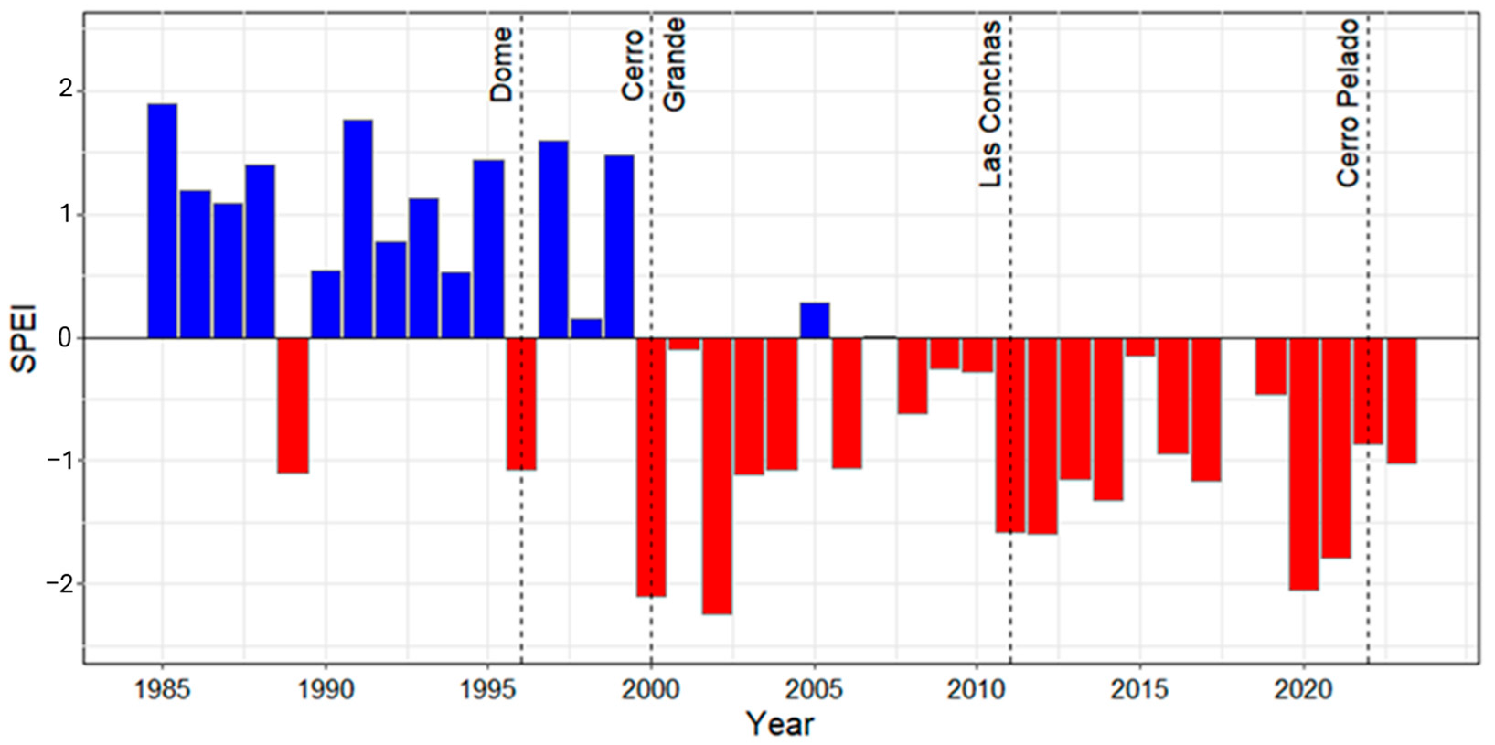
This study was located in the eastern Jemez Mountains of northern New Mexico (Figure 1). The regional climate is characterized as semi-arid and continental, with cold winters and hot, monsoonal summers [42]. The study area ranges in elevation from approximately 1600 m to 3300 m. Mid-elevations feature ponderosa pine (Pinus ponderosa) intermixed with aspen (Populus tremuloides) and shrublands of New Mexico locust (Robinia neomexicana) and a mix of Gambel oak (Quercus gambelii) and Wavyleaf oak (Quercus pauciloba) [43], which will hereafter be referred to as ‘oak’ in this study. We assessed regional drought severity over recent decades using the standardized precipitation evapotranspiration index (SPEI), revealing a prolonged drought since the year 2000 (Figure 2).
The study area encompasses the perimeters of three major fires, covering nearly 74,000 hectares in total (Figure 1). The Dome Fire (April 1996) burned nearly 6500 hectares of land, the Cerro Grande Fire (May 2000) burned over 17,000 hectares, and the Las Conchas Fire (June 2011) burned over 63,000 hectares of the landscape, reburning areas burned in previous fires [44]. The Cerro Pelado Fire occurred within the study period from April 22–June 15 in 2022, burning 18,500 hectares, largely at low severity [45].
Figure 2. Standardized precipitation evapotranspiration index (SPEI) for the study area. The SPEI calculates the climatic water balance by comparing precipitation and potential evapotranspiration, expressed as a standard deviation from the long-term mean (1895-present) [46]. SPEI data were obtained from the Western Regional Climate Center (http://www.wrcc.dri.edu; accessed on 18 December 2023). Years in red indicate a lower SPEI than the long-term mean (1895-present), while years in blue indicate a higher SPEI than the long-term mean. Vertical dashed lines mark the years and names of major fires within the study area.
Land 14 01603 g002

2.2. Study Design and Data Aquisition

Figure 3 illustrates the methodology used to estimate fractional shrub cover. The method involves deriving fractional cover estimates from classified NAIP imagery in 10 × 10 m and 20 × 20 m grids. These estimates are then used as inputs for random forest models, which are built using spectral, topographic, and burn variables resampled to 10 and 20 m for the respective models. After comparing the 10 m and 20 m models, the model with the lowest error was selected to estimate DFSC for the years 2019–2023, to be used in further analysis of DFSC change.
We visited the study site in mid-June of 2023 to collect geo-referenced photos at 69 different locations. We interpreted NAIP imagery referencing the photos from the field to create a field-validated dataset of shrub presence and absence points, resulting in 422 field-validated points.
Aerial and satellite imagery were accessed in Google Earth Engine (GEE) and USGS Earth Explorer. We used 0.6 m resolution National Agriculture Imagery Program (NAIP) imagery from 6-6-2020, to generate a shrub-presence basemap from which fractional vegetation cover was derived. Imagery from 6-14-2022 was used for the accuracy assessment of the 2022 model predictions.
Spectral variables were derived from Sentinel-2 atmospherically corrected L2A imagery and Sentinel-1 SAR GRD imagery. Leaf-on data was collected from June 1–August 31, and leaf-off images were collected from October 10 to November 30. Image collections were filtered to include images with 20% or less cloud cover, and a cloud mask was applied to remove any remaining cloudy pixels. We also included Sentinel-1 C-Band Synthetic Aperture Radar (SAR) VV and VH bands, as these bands are sensitive to vegetation structure and canopy complexity [47], and have demonstrated potential for distinguishing coniferous from deciduous forest types [48].
Topographic variables, including elevation, slope, aspect, and topographic position index (TPI) were derived from the USGS 1/3 arc-second Digital Elevation Model (DEM) product (USGS/3DEP/10m) available in GEE. Heat Load Index (HLI) was collected from the Global ALOS Continuous Heat-Insolation Load Index (CHILI) in GEE [49]. Elevation and other terrain-based landscape features are correlated with species distribution, climate variability and vegetation patterns [6,21,50], making them important predictors of vegetation change.
Burn variables and fire perimeters were derived from Monitoring Trends in Burn Severity (MTBS) burn severity maps. High burn severity and repeat fire are drivers of forest conversion [5,15,27] and promote growth and establishment of resprouting shrub species [4,51], making them relevant variables in this study.

2.3. Explanatory Variables

All 10 and 20 m spectral bands from Sentinel-2 were included as variables, as well as the Normalized Vegetation Index (NDVI) and Enhanced Vegetation Index (EVI) [52,53]. The average spectral values were calculated for leaf-on and leaf-off periods, and standard deviation was calculated over the entire period (June 1–November 30). All variables (Table 1) were either collected at or resampled to 10 and 20 m (using bilinear interpolation), resulting in two sets of the same variables. Spectral variables with a native resolution of 10 m were collected at their native resolution, and scaled up to 20 m in GEE, and variables available at 20 m were downscaled to 10 m. Topographic variables, available in GEE at 30 m resolution, were resampled to 10 and 20 m.
The probability of shrub presence was included as a predictor variable (Figure 3) to address zero-inflation in the model, which would be caused by the majority of sample points having low shrub cover, which is typical in arid regions. This was calculated by creating an initial random forest model to predict the probability of shrub presence in a given pixel, using the same spectral, topographic and burn variables. Remotely sensed variables and indices can have high correlation [54], which can inflate statistical models and lead to less accurate predictions. Therefore, we tested for and removed collinear variables. Then, we pruned the models using a backwards stepwise selection, in which the least significant variable was removed until the model stabilized, and no further variables could be removed without significantly worsening the model’s performance [46].

2.4. Shrub-Presence Basemap

We generated a high-resolution shrub-presence basemap using 0.6 m NAIP imagery from 2020. The NAIP imagery was classified in QGIS using the unsupervised K-means clustering algorithm with spectral angle distances. The classifier was configured to produce 30 distinct spectral classes, which were interpreted as either shrub or non-shrub using photointerpretation and by referencing the GPS-tagged field photos. We performed an accuracy assessment on the basemap using the field-validated dataset. Accuracy was evaluated using the F1 score, which reflects the balance between precision and recall, providing a measure of classification performance [55].
Table 1. Covariates used in random forest models. USGS = United States Geological Survey, CSP = Conservation Science Partners, MTBS = Monitoring Trends in Burn Severity. Leaf-on, leaf-off, and standard deviation of all spectral variables were used.
VariableDescriptionSource
SpectralBand 2Blue band—490 nmSentinel-2 (GEE)
Band 3Green band—560 nm
Band 4Red band—665 nm
Band 5Red edge 1—705 nm
Band 6Red edge 2—740 nm
Band 7Red edge 3—783 nm
Band 8Near-infrared (NIR)—842 nm
Band 8aNarrow NIR—865 nm
Band 11Short wave infrared (SWIR 1)—1610 nm
Band 12SWIR 2—2190 nm
NDVINDVI = (B8 − B4)/(B8 + B4) [56]
EVIEVI = 2.5 * ((B8 − B4)/(B8 + 6 * B4 − 7.5 * B2 + 1)) [57]
Sentinel-1 VV and VHC-band Synthetic Aperture RadarSentinel-1 (GEE)
TopographicElevationDerived from National elevation datasetUSGS (GEE)
SlopeDerived from National elevation dataset
AspectDerived from National elevation dataset
HLIDerived from Global ALOS CHILI dataset, a measure of incident radiation [58]CSP (GEE)
TPIDerived from National elevation dataset, a measure of elevation relative to surrounding cells [59]USGS (GEE)
BurnTime since burnYears since last burnMTBS
Burn severityBurn severity maps from MTBS
Number of times burned
Probability of shrub presence
(probShrub)
Probability that shrubs are present in a given pixel

2.5. Fractional Shrub Cover Estimation

To estimate fractional shrub cover, we first created sample points following methods described in Assal et al. [60]. The study area was classified into 12 landscape facets based on three elevation levels and four aspect directions (north, east, south, and west). Then we applied a stratified random sampling procedure in R using the dplyr [61] package to ensure even distribution of points across facets. This approach aimed to encompass a range of environmental conditions and reduce spatial dependency. Sample points were constrained by a minimum distance of 300 m between points, yielding 646 sample points.
Fractional shrub cover was then derived from the shrub-presence basemap using methods adapted from Warkentin et al. [62]. The sample points were converted to raster pixels aligned with 10 m and 20 m Sentinel-2 images. These pixels were then converted to 10 × 10 m and 20 × 20 m plots, in which percent shrub cover was calculated. The centroid of each plot containing the percent of shrub cover, or DFSC value, was used in random forest model training.

2.6. Random Forest Models

Two random forest models were built in R (R Core Team, 2023) using the randomForest [63] package: one model utilized 10 m resolution variables, while the other employed 20 m resolution variables. Random forest models are known for achieving high accuracy even in complex forest types [64,65], making them a popular choice for estimating fractional vegetation cover [34,66].
The random forest models were built from 2020 satellite imagery, yielding a 10 and a 20 m model for the year 2020. Each model was trained using 1001 trees (ntree = 1001) and three variables selected at each split (mtry = 3). The nodesize and maxnodes parameters were left unspecified and thus defaulted to the package settings, which allow trees to grow until reaching a minimum terminal node size of one (for classification) without a predefined limit on the number of terminal nodes. Variable importance scores were enabled during training. We tested for multicollinearity and pruned the models using the same methods described in Section 2.4. Out-of-bag (OOB) error was used as an internal validation measure during model training, yielding a mean squared error of 61.64 and 82.01% variance explained.
Model performance was evaluated using root-mean-squared error and R-squared [67,68]. The model with the best performance according to these metrics was used to generate yearly DFSC predictions [69]. To do this, spectral variables were replaced with those from the respective year. This process resulted in yearly DFSC predictions, with each pixel being scaled between 0 and 100% to reflect estimated shrub cover.
We evaluated the accuracy of the 2022 DFSC predictions using NAIP imagery from the same year. The NAIP imagery was classified according to the method outlined in Section 2.5. We randomly generated 352 points in QGIS, with a minimum distance of 300 m between each point. DFSC values were extracted at each point as described in Section 2.6, to serve as ground-truth data for comparison with the prediction. The prediction’s accuracy was assessed using simple linear regression, from which R-squared, RMSE and MAE were calculated [67].
We also analyzed the impact of several environmental factors (burn severity, elevation, and aspect) using a Kruskal–Wallis test on a 5% random sample from each group. The Kruskal–Wallis test was used to assess the significance of elevation and aspect [70], which had three and four groups, respectively, and the Mann–Whitney U test was used to assess the significance of number of times burned, which only had two groups [71]. We analyzed the significant differences between groups using an ANOVA with multi-comparison post hoc Tukey’s HSD test.

2.7. Trend Analysis

To analyze shrub cover change over the study period, we tested for significant monotonic trends using the Mann–Kendall test and the Theil–Sen median trend test. The Mann–Kendall test is a non-parametric statistical method used to assess the significance of trends over time [72]. The Theil–Sen median trend test, also non-parametric, calculates the median slope between all pairs of points in the time series [73]. These methods have been used in tandem to analyze vegetation change [46,74]. These tests were applied using the modifiedmk [75] package in R to quantify the magnitude and direction of change. The pwmk function uses methods from Von Storch, [76] to handle small sample sizes (n < 10) by prewhitening the data using the lag-1 serial correlation coefficient to account for temporal correlation.
Following the methods outlined in Assal et al. [11] we used a Generalized Linear Model (GLM) to analyze the relationship between trends and environmental facets. We assessed the effect of the number of times burned, burn severity, elevation, HLI and TPI. We used a weighted sampling method, selecting a 10% random sample from significant positive trends, significant negative trends, and pixels with no significant trend. Then, we calculated the effect size of each explanatory variable by calculating the predicted magnitude of slope at the 25th percentile (Q1) and 75th percentile (Q3), holding other variables constant at their mean, and calculating the effect size as the difference between predictions at Q1 and Q3 [77]. This allowed for a comparison of their relative importance on a common scale, facilitating easier interpretation of their individual impacts. As a discrete indicator variable, the number of times burned was not included in the scaled effect analysis.

3. Results

3.1. Basemap and Random Forest Models

The basemap had an overall accuracy of 96.4%, and the F1 scores for the shrub and non-shrub classes were 0.97 and 0.95, respectively, indicating high accuracy for both. The 20 m RF model had an RMSE of 7.85, and an R-squared value of 0.82, while the 10 m model had an RMSE of 9.99 and an R-squared of 0.76. Therefore, the 20 m model was used for yearly predictions of DFSC and further analysis.

3.2. Variable Importance

Variable importance remained relatively consistent across scales (Figure 4). In both models, probShrub, NDVI, NDVIsd, and EVIsd ranked among the top six most important variables. A variation in one of the red-edge bands was highly important in each model: B6 for the 20 m model and loB5 for the 10 m model. Variations in the red band also ranked highly: B4 and loB4 for the 20 m model, and B4sd for the 10 m model. Elevation and loB11 were also important for each model, though they ranked lower in both.

3.3. DFSC Prediction Accuracy

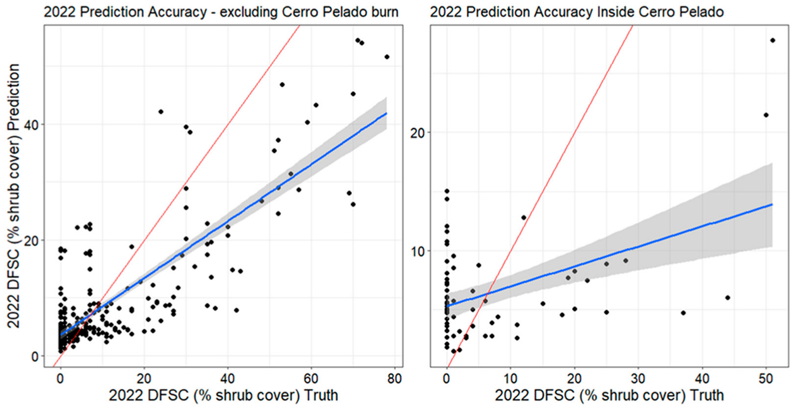
The 2022 DFSC prediction achieved an overall R-squared value of 0.62, RMSE of 10.11, and an MAE of 6.99. When only testing areas outside the Cerro Pelado burn scar, the R-squared value improved to 0.67, RMSE decreased to 9.96, and MAE decreased to 6.97. Within the Cerro Pelado burn scar, DFSC predictions were largely overestimated, resulting in an R-squared of just 0.21 for that area (Figure 5).

3.4. Interannual Variation in DFSC

The yearly global mean of DFSC decreased from 14.4% in 2019 to 7.6% in 2022, then increased to 16.6% in 2023. Figure 6 illustrates the net change from 2019 to 2023. In the net change map, 49.7% of the area showed a positive value (increase in DFSC), while 51.2% showed a negative value (decrease in DFSC). Despite this, the average net change was 2.2%, indicating an overall increase in DFSC. The average increase in DFSC for positive pixels was 8.25%, whereas the average decrease for negative pixels was −3.77%. The average increase in positive pixels inside the Cerro Pelado burn scar was 11.6%.
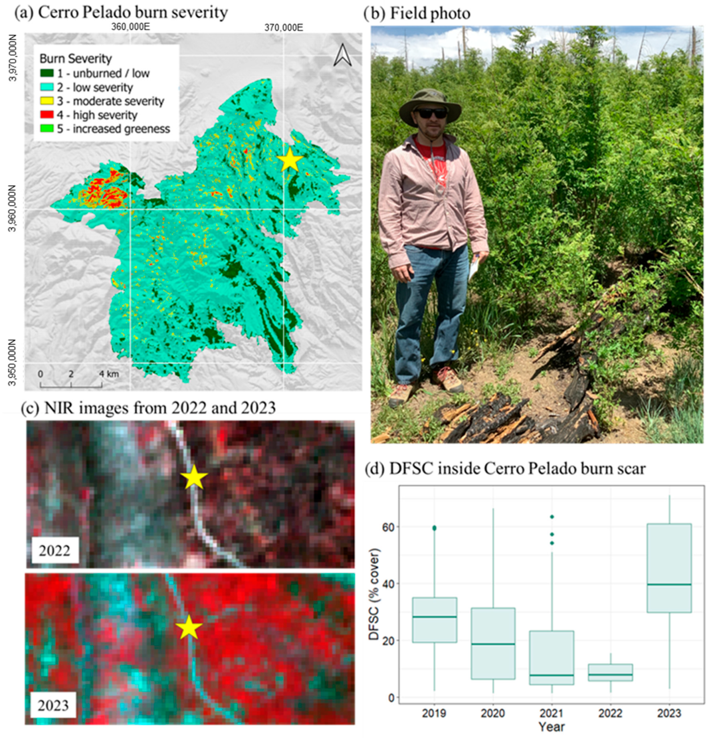
In 2019, the total shrub cover was 10,064 hectares, which increased to 11,605 hectares in 2023, indicating a total increase of 1541 hectares over the five years. Although the Cerro Pelado burn scar covers only about 25% of the study area, it contributed nearly 66% (1014 hectares) of the DFSC increases across the entire region. Yearly predictions of DFSC within the Cerro Pelado burn scar are shown in Figure 7d.
To eliminate added variability introduced by the fire, we further analyzed DFSC outside and inside the Cerro Pelado (CP) burn scar separately. Yearly total shrub cover in areas outside of Cerro Pelado are shown in Table 2. To quantify model uncertainty, we calculated per-pixel standard deviation (SD) from predictions generated by all trees in a random forest model. SD values were computed across individual tree predictions for each pixel and then mapped back to spatial form as a raster, yielding a mean SD of 7.05 in areas outside of Cerro Pelado. The uncertainty raster from 2020 was adopted as a global SD estimate and applied uniformly across all years of the study. Appendix A contains supplementary analyses that detail additional metrics related to model uncertainty. Global means of DFSC outside of the CP burn scar were similar to those of the entire study area, decreasing from 2019 to 2022, then increasing in 2023. Even outside of the CP fire, 2022 experienced the greatest loss in shrub cover, losing 1694 hectares from the previous year. Figure 8 shows an area of substantial shrub loss, with NAIP imagery and DFSC predictions from 2020 and 2022 in the same location.
The impact of elevation, aspect, burn severity and number of times burned on DFSC were evaluated in areas unaffected by the CP fire. Each environmental factor was significant (p < 0.05), with the highest DFSC observed at mid-elevations, on north and east-facing slopes, in areas with higher burn severities, and in regions that experienced multiple burns.
We evaluated the impact of several environmental factors on DFSC change outside of the CP burn. Each group was significantly different (p < 0.05). The highest DFSC was observed at mid-elevations, on north and east-facing slopes, in areas with higher burn severities, and in regions that experienced multiple burns. Figure 9 shows the yearly relationship between elevation and DFSC.

3.5. Trend Analysis

Without considering statistical significance, 58.1% of pixels exhibited a positive trend, while 41.9% showed a negative trend over the 5-year period. Approximately 5% of pixels had a statistically significant trend (p < 0.1), with 83.0% showing a positive trend and 17.0% exhibiting a negative trend.
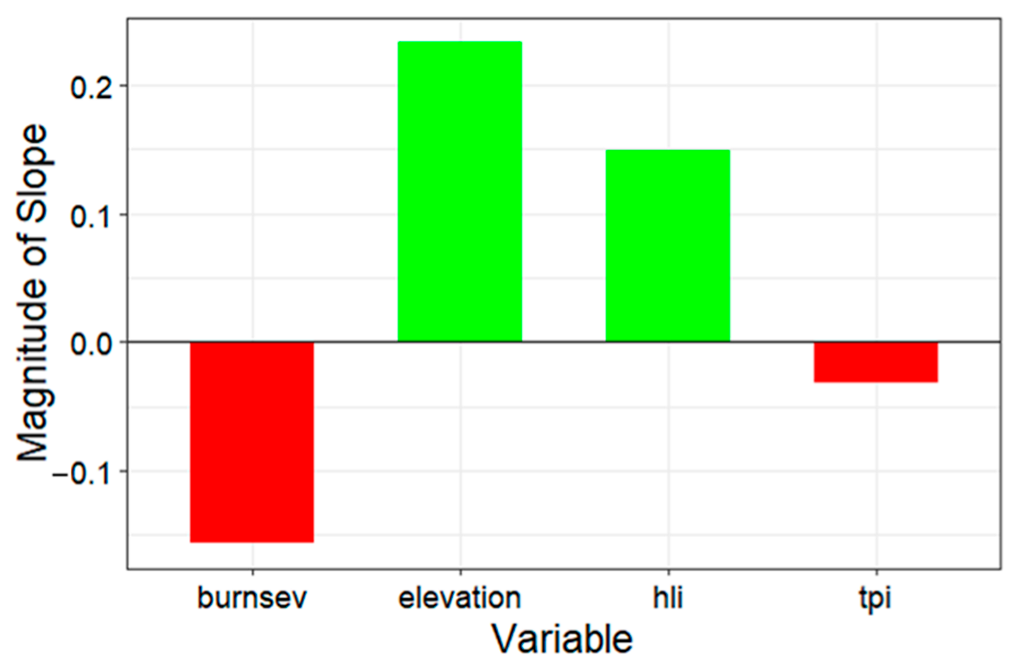
The effect of number of times burned, burn severity, elevation, HLI, and TPI were each statistically significant at the 95% confidence level. Elevation and HLI were associated with positive trends, while the number of times burned, burn severity, and TPI were associated with negative trends. The scaled effects of the variables are shown in Figure 10. Not including number of times burned, elevation had the greatest relative effect, followed by burn severity, HLI, and finally TPI.

4. Discussion

In this study, we assessed the impact of scale on modeling fractional shrub cover and evaluated interannual changes and overall trends in DFSC. The 20 m random forest model outperformed the 10 m model in predicting DFSC. Variable importance was largely unaffected by scale, with the probability of shrub presence and NDVI being the most significant variables regardless of scale. Yearly DFSC predictions revealed a decrease from 2019 to 2022, coinciding with drought and the Cerro Pelado fire in 2022, followed by an increase from 2022 to 2023. DFSC increased disproportionately within the CP burn scar. The trend analysis revealed that most of the pixels with significant slopes were positive and were correlated with topographic and burn variables. Despite considerable interannual variability during a time of drought and wildfire, fractional shrub cover generally increased.

4.1. Scale Affects Random Forest Model Performance

Model scale was found to have a notable impact on performance, with the 20 m model exhibiting a higher R-squared and lower RMSE than the 10 m model. Variable importance was similar, with some of the most important variables in each model being probability of shrub presence, NDVI, and NDVIsd. The probability of shrub presence was the most significant variable in each model (Figure 4) which was expected. If there is a high likelihood of shrub presence, it is likely that there will be some percentage of shrub cover. This variable was derived from a random forest model using the same input variables as the 10 m and 20 m models; consequently, it interacts with spectral and environmental predictors that are crucial for shrub presence and, by extension, are likely significant for shrub cover as well. Longitude was also highly important in the 20 m model, as it reflects an elevation change from east to west in the study area. As longitude decreases from east to west, more mesic conditions support increased shrub growth more than lower, arid conditions.
Derived indices were also important, as expected, as they have a strong correlation with fractional vegetation cover [78,79]. These are commonly used to evaluate vegetation recovery following wildfire [80,81,82]. NDVIsd can help distinguish deciduous species from coniferous species, as NDVI values for deciduous species are high in the summer and low in the winter, but remain relatively consistent for coniferous species. EVIsd was also important, ranking higher in the 20 m model. EVI may also help distinguish deciduous from coniferous species, as it is sensitive to dense biomass-conifers maintain similar biomass throughout the seasons, whereas deciduous species’ biomass reduces when leaves abscise. A coarser resolution may offer a more homogeneous signal that better represents overall vegetation density, compared to a finer resolution.
The red-edge bands were found to be important in both models (Figure 4). Red-edge 2, or band 6 was important in the 20 m model, and leaf-off red-edge 1 (loB5) was important in the 10 m model. The red-edge bands have shown a strong relationship with fractional vegetation cover [30,38,39]. Red-edge 1 (705 nm) is at the lower range of the red edge, making it highly sensitive to variations in vegetation/chlorophyll content [83] which may be better captured in higher resolution 10 m imagery. Red-edge 2 (740 nm) in the middle of the edge may capture slightly broader trends in the 20 m imagery, relating to more general vegetation health. Regardless of scale, the red-edge bands appear to be relevant to modeling DFSC. This highlights the advantage of Sentinel-2 having three bands in this range, which can detect small variations at multiple scales.
Based on the importance of variables and the spatial scale of landscape features and shrub growth properties, the 20 m resolution imagery is more effective at capturing overall vegetation cover. The higher 10 m resolution appears to miss broader trends, such as topographic variation, which is a crucial indicator of shrub cover. It is possible that coarser resolution imagery more accurately captures shrub cover because shrubs often occur in large, aggregated patches. While higher resolution imagery provides more detail, it can introduce additional noise, making it harder to distinguish these shrub patches. In contrast, the coarser resolution cannot pick up as many high-detail variations, offering a better overall representation of shrub cover. Using a coarser resolution is also more practical for computational time in a large landscape, where capturing the overall extent of the shrubs is more essential than identifying minute differences in individual shrubs. This aligns with other studies that have found 20 m Sentinel-2 imagery effective for estimating fractional vegetation cover in semi-arid regions [34] and specifically for estimating fractional shrub cover [33]. Warkentin et al. [62] also found that estimating shrub cover from 20 m grids was more accurate than from 10 m grids, while still providing a fine enough resolution to detect changes in shrub growth.

4.2. DFSC Has High Interannual Variation with Overall Increasing Trends

DFSC showed a decrease in shrub cover from 2019 to 2022, followed by a drastic increase in 2023. These trends were consistent in both the Cerro Pelado burn scar and areas unaffected by that fire (Table 2).The overall net change indicated an increase in DFSC despite the five years being significantly impacted by drought and wildfire, which caused a consistent decrease for most of the study period. The study area experienced severe drought conditions in 2020 and 2021 (Figure 2), preceding the Cerro Pelado fire in 2022. Drought conditions in these years were the most severe since 2002 (Figure 2). Although oak and New Mexico locust are highly resistant to drought conditions [17,22] even these resilient species showed signs of stress during that time (Figure 9). Following 2021, the study area continued to experience below-average SPEI, albeit with less severity. This could have supported the recovery and significant increase in shrub cover by 2023.
The trend analysis revealed that 58% of pixels in the study area experienced an increase in DFSC. The global mean of the entire study area was 2.2%, indicating a positive trend on average. Only 5% of slopes were statistically significant, which is expected, considering there was a substantial decrease in shrub cover followed by a significant increase, resulting in most of the landscape showing no trend. Of the significant slopes, 83% were positive, indicating an increase in shrub cover. Although five years is a short period for observing landscape scale changes, the presence of significant slopes within this period underscores the persistent nature of the shrubs. Oak and New Mexico locust have high drought tolerance and fire resilience [17,22], and post-fire vegetation has been shown to be even more resilient to subsequent fire [27]. Past high-severity fire, climate change and current fire regimes promote persistence of altered post-fire vegetation states, especially those comprising resprouting shrub species [15,26]. These findings suggest that shrub cover is likely to continue to increase during periods of fire and extreme drought, demonstrating its persistence and potential for continued expansion as a relatively stable vegetation state in this landscape.

4.3. Environmental Variables Drive DFSC Trends

The relationship between shrub cover trends and environmental factors was assessed using the scaled effect on slope magnitude (Figure 10). Elevation and HLI were associated with positive trends (p < 0.05), while number of times burned, burn severity and TPI were associated with decreasing trends (p < 0.05). Elevation had the largest relative impact on shrub growth trends, with higher elevations correlating with positive trends and the highest DFSC predictions occurring at moderate and high elevations (Figure 9). Cooler climates and more mesic conditions at higher elevations offer more favorable conditions for vegetation growth, resulting in increased post-fire regeneration. Several western landscapes have demonstrated better post-fire forest recovery at higher elevations compared to lower elevations [15,84,85].
Burn severity and number of times burned were both associated with decreasing shrub cover trends. While burn severity is a significant driver of forest-to-shrubland conversion [15,27], the last burn (Las Conchas, 2011) occurred eight years before this study, suggesting its influence on shrub expansion has diminished. Additionally, areas outside the Cerro Pelado burn were mainly affected by the Cerro Grande Fire (2000) and the Las Conchas Fire (2011) (Figure 1). The Las Conchas Fire burned mostly at moderate and high severities across elevations. Similarly, the Cerro Grande Fire burned largely at moderate and high severities, but at low and moderate elevations. Areas that experienced overlap from these fires were situated at moderate to lower-range high elevations. These patterns likely result in the number of times burned and burn severity having inverse relationships with shrub cover trends. Lower elevations, which experience warmer, drier conditions, face even greater limitations to vegetation recovery when coupled with intense drought, especially following severe, repeated fire [21,50,85]. This hypothesis is supported by Figure 8, which shows an area of substantial decrease in DFSC. This patch occurred in the area burned by both Las Conchas and Cerro Grande and sits at a lower elevation. This loss of shrub cover can likely be explained by the overlap of high-severity fires and the climate associated with lower elevations, which are particularly affected by drought.
HLI showed a positive relationship with trends, as higher HLI values occur on south- and west-facing, steeper slopes due to increased direct sunlight, leading to warmer and drier conditions. Conifer forests struggle to regenerate in these topographies and associated microclimates [80,85], likely reducing competition for shrubs. Cocking et al. [51] found that HLI was associated with decreased post-fire mortality of resprouting California black oak in Northern California [51], suggesting that higher HLI may enhance the recovery of resprouting species. At higher elevations, where conditions are cooler and moister, increased direct sunlight may create highly favorable conditions for shrubs.
TPI was associated with decreasing trends. Areas with high TPI, such as ridges or hilltops, face similar challenges to steep slopes, like limited water availability and increased burn severities [86]. High TPI has been associated with low levels of post-burn recovery in both conifer forests [80] and resprouting deciduous species [87].

4.4. Effects of Recent Fire on DFSC Dynamics

Changes in DFSC within the Cerro Pelado burn scar were analyzed with yearly DFSC predictions, as no trends can be detected over a 1 year period. The global mean of DFSC within the Cerro Pelado fire was just 6.6% in 2022 after the fire and jumped to 20.7% in 2023. Considering the total net change from 2019 to 2023 (Figure 6), the area affected by Cerro Pelado contributed 66% of the total area of shrub cover increase, although Cerro Pelado covered only 25% of the study area. The change in DFSC over the study period can be seen in Figure 7d, decreasing until 2022 and increasing drastically in 2023.
The drought conditions in 2023 were less severe, likely facilitating shrub recovery following the burn. A significant increase in healthy vegetation can be seen just one year post-fire in a color-infrared image from the Cerro Pelado fire (Figure 7c). A field visit in June 2023 confirms rapid resprouting and/or refoliation in that area, where New Mexico locust shrubs were over six feet tall (Figure 7b). Cerro Pelado primarily burned over areas previously affected by the 2011 Las Conchas fire, which likely contributed to its low severity [27]. Areas burned at lower severity have shown increased short-term regeneration [81], where most regrowth typically occurs within the first three years following a disturbance [27,81,82]. Therefore, it is not surprising that significant growth was observed, especially given the less severe drought conditions in 2023 (Figure 7).
The 2022 DFSC predictions significantly overestimated DFSC within the CP burn scar, resulting in an R-squared of just 0.21. Many points with zero ground-truth cover were predicted to have 0–20% DFSC, with about 64% of points being overpredicted (Figure 5). The NAIP imagery used for ground-truth points was taken on 14 June 2022, just before Cerro Pelado was officially considered under control on 15 June. In contrast, the Sentinel-2 imagery for DFSC predictions spanned from 1 June to 31 August, potentially capturing early shrub regrowth. This likely led to the overprediction of shrubs in the field-derived dataset, particularly in areas affected by Cerro Pelado.

4.5. Ecological and Technical Considerations

As previously mentioned in Section 4.4, there was a timing discrepancy between the NAIP and Sentinel-2 imagery. The NAIP imagery for the binary species distribution basemap was taken on 6 June 2020, and the NAIP imagery for the 2022 accuracy assessment was taken on 14 June 2022. In contrast, the Sentinel-2 imagery for DFSC predictions was gathered between 1 June and 31 August for the leaf-on imagery. This timing difference could have led to an apparent overprediction of DFSC, as the baseline data was taken earlier in the season. This discrepancy particularly impacted the 2022 prediction accuracy assessment within the Cerro Pelado burn scar (Figure 5), where prolific resprouting of deciduous shrub species would be expected following the disturbance. At the time of this study, development of a unique shrub cover basemap was more effective than using existing fractional vegetation cover products [39,40]. A new RAP product that utilizes Sentinel-2 data (10 m) and has additional PFTs is expected to be released in 2025 [88]; however, DSFC is not one of the new plant functional types. Future research should assess this product’s efficiency in shrub cover prediction in this system that has unique PFTs. Other methodological approaches, such as integrating auxiliary datasets—like soil moisture or LAI time series—could help temporally harmonize imagery and improve assessment accuracy. However, the coarse spatial resolution of these datasets (typically >100 m) limits their direct applicability to our model outputs at 20 m resolution. Nonetheless, future efforts to explore multiscale data integration for temporal harmonization could help refine shrub regeneration predictions in dynamic post-fire landscapes.
This study used bilinear interpolation to resample continuous data layers, a method widely used in ecological remote sensing. Compared to alternatives like nearest neighbor or bicubic, bilinear offers reliable performance with lower computational demand [89]. While advanced techniques such as bicubic interpolation or Hopfield Neural Network (HNN) resampling may yield more accurate results, they also require significantly more computation [90]. The influence of alternative resampling methods on study outcomes warrants further investigation in future work.
Another limitation was the missing data in the burn severity mosaic for the Las Conchas fire, caused by the Landsat 7 Scan Line Corrector (SLC) failure. This technical issue resulted in stripes of missing data in each scene, omitting key information. Since the Las Conchas burn scar constituted the majority of the study area and was the most recent fire before Cerro Pelado, the burn severity variable was greatly impacted by the missing data.
The Cerro Pelado Fire in 2022 presented both challenges and opportunities for this study. Nearly 25% of the study area had to be excluded from certain analyses. However, the large size and environmental variability of the remaining areas provided valuable information covering a wide range of conditions. Additionally, the fire offered a unique opportunity to assess vegetation change one year post-fire.
Additionally, this study treated deciduous resprouting shrubs as a single functional group characterized by two time periods of reflectance within a single year. Incorporating all satellite observations within a calendar year holds promise to disentangle these conspicuous deciduous species [91]. However, additional satellite observations require more sophisticated statistical analyses as well as intensive processing power before such an approach is operational at the landscape scale.
Finally, the short time frame of this study posed several limitations. It restricted the amount of data that could be collected, thereby reducing the statistical power of trend analysis. Level-2A Sentinel-2 imagery is only available in this study area from 2019 onward. While Level-1 top of atmosphere (TOA) imagery is available, it requires processing to eliminate atmospheric effects. We chose to use only Level-2A imagery because atmospherically correcting Level-1 imagery is computationally difficult and can introduce errors. Additionally, using both types of imagery could introduce inconsistencies. The Mann–Kendall Theil–Sen trend analysis can detect trends with as few as three time periods [92], but a longer time span would give a better understanding of shrub cover change over time. However, we implemented a modified version of the Mann–Kendall test [75,76] recommended in small sample sizes (n < 10) to account for temporal autocorrelation that is more influential in shorter time series. Despite this challenge, this study highlighted the dynamic yearly variability in this system and provided a close look at post-fire regeneration patterns in deciduous resprouting shrubs. Future analyses can revisit the approach and results of this study as the vegetation continues to develop on the post-disturbance environment.

5. Conclusions

The increasing evidence that post-conversion vegetation types are long-term or permanent states highlights the need to monitor and understand the dynamics of unique vegetation types to effectively manage landscapes [13,15]. This study revealed high interannual variability with overall increasing trends of shrub cover, despite drought conditions and a major wildfire during the study period. Areas affected by the fire exhibited significant regrowth within one year. Elevation was a key driver of DFSC trends, and the red-edge bands were important variables at both scales.
Our findings underscore the resilience of deciduous shrubs to repeated disturbances and their tolerance to adverse climate conditions, as observed in other studies [18,19,27]. This resilience, combined with species competition and adverse climate conditions, poses compounding challenges to conifer recruitment [4,13]. Consequently, the persistence of shrubs under these conditions adds further evidence that deciduous shrubland may represent a long-term stable vegetation state in this landscape [6].
Our findings offer valuable insight into post-disturbance land management. Spatial and temporal patterns of shrub recovery can help identify zones where additional monitoring or intervention may be warranted. The methodologies applied in this study offer land managers an efficient means of tracking vegetation dynamics and guiding resource allocation. As vegetation shifts with changing climate and fire regimes, management strategies will need to prioritize adaptive approaches. Recognizing these changes and adjusting practices accordingly will be crucial for sustaining long-term ecosystem health.

Author Contributions

Conceptualization, H.T. and T.A.; methodology, H.T. and T.A.; formal analysis, H.T. and T.A.; data curation, H.T.; writing—original draft preparation, H.T. and T.A.; writing—review and editing, H.T. and T.A.; visualization, H.T. and T.A.; supervision, T.A. All authors have read and agreed to the published version of the manuscript.

Funding

This research received no external funding.

Data Availability Statement

All satellite data used in this study are publicly available through Google Earth Engine. Field-collected data has been archived in the Knowledge Network for Biocomplexity [93]. R code for analysis is available from the corresponding author upon request.

Acknowledgments

We thank Andreas Wion, Ellis Margolis, and Craig Allen for field assistance and collaboration. We gratefully acknowledge financial support from the Department of Geography at Kent State University.

Conflicts of Interest

The authors declare no conflicts of interest.

Appendix A

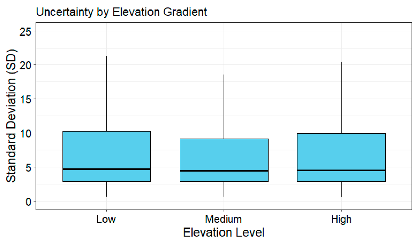
To evaluate spatial variability in model uncertainty, we summarized per-pixel standard deviation (SD) across the study area, in areas outside of Cerro Pelado. Key statistics included the mean Standard Deviation (7.05), 25th percentile (2.87), 50th percentile (4.56), and 75th percentile (9.94), which together indicated a moderately skewed but relatively uniform spread of prediction uncertainty. When stratified by elevation levels, boxplots showed similar distributions across elevation zones. A one-way ANOVA test (p = 0.199), followed by Tukey’s HSD post hoc comparisons, revealed no statistically significant differences in SD between elevation groups. This suggests elevation did not influence model uncertainty, and that prediction confidence was broadly consistent across the landscape’s vertical gradient.
Figure A1. Standard Deviation by elevation, outside of the Cerro Pelado burn scar. 1 = low elevations (1660–2341 m), 2 = mid-elevations (2341–2679 m), and 3 = high elevations (2679–3358 m).
Land 14 01603 g0a1

References

  1. Abatzoglou, J.T.; Williams, A.P. Impact of anthropogenic climate change on wildfire across western US forests. Proc. Natl. Acad. Sci. USA 2016, 113, 11770–11775. [Google Scholar] [CrossRef]
  2. Mueller, S.E.; Thode, A.E.; Margolis, E.Q.; Yocom, L.L.; Young, J.D.; Iniguez, J.M. Climate relationships with increasing wildfire in the southwestern US from 1984 to 2015. For. Ecol. Manag. 2020, 460, 117861. [Google Scholar] [CrossRef]
  3. Steel, Z.L.; Safford, H.D.; Viers, J.H. The fire frequency-severity relationship and the legacy of fire suppression in California forests. Ecosphere 2015, 6, 1–23. [Google Scholar] [CrossRef]
  4. Haffey, C.; Sisk, T.D.; Allen, C.D.; Thode, A.E.; Margolis, E.Q. Limits to Ponderosa Pine Regeneration following Large High-Severity Forest Fires in the United States Southwest. Fire Ecol. 2018, 14, 143–163. [Google Scholar] [CrossRef]
  5. Savage, M.; Mast, J.N.; Feddema, J.J. Double whammy: High-severity fire and drought in ponderosa pine forests of the Southwest. Can. J. For. Res. 2013, 43, 570–583. [Google Scholar] [CrossRef]
  6. Guiterman, C.H.; Margolis, E.Q.; Allen, C.D.; Falk, D.A.; Swetnam, T.W. Long-Term Persistence and Fire Resilience of Oak Shrubfields in Dry Conifer Forests of Northern New Mexico. Ecosystems 2018, 21, 943–959. [Google Scholar] [CrossRef]
  7. Williams, A.P.; Cook, B.I.; Smerdon, J.E. Rapid intensification of the emerging southwestern North American megadrought in 2020–2021. Nat. Clim. Chang. 2022, 12, 232–234. [Google Scholar] [CrossRef]
  8. Garfin, G.; Jardine, A.; Merideth, R.; Black, M.; LeRoy, S. (Eds.) Assessment of Climate Change in the Southwest United States: A Report Prepared for the National Climate Assessment; Island Press/Center for Resource Economics: Washington, DC, USA, 2013. [Google Scholar] [CrossRef]
  9. Hessburg, P.F.; Prichard, S.J.; Hagmann, R.K.; Povak, N.A.; Lake, F.K. Wildfire and climate change adaptation of western North American forests: A case for intentional management. Ecol. Appl. 2021, 31, e02432. [Google Scholar] [CrossRef]
  10. Allen, C.D.; Breshears, D.D.; McDowell, N.G. On underestimation of global vulnerability to tree mortality and forest die-off from hotter drought in the Anthropocene. Ecosphere 2015, 6, 1–55. [Google Scholar] [CrossRef]
  11. Assal, T.J.; Anderson, P.J.; Sibold, J. Spatial and temporal trends of drought effects in a heterogeneous semi-arid forest ecosystem. For. Ecol. Manag. 2016, 365, 137–151. [Google Scholar] [CrossRef]
  12. Tepley, A.J.; Thomann, E.; Veblen, T.T.; Perry, G.L.W.; Holz, A.; Paritsis, J.; Kitzberger, T.; Anderson-Teixeira, K.J.; Lines, E. Influences of fire–vegetation feedbacks and post-fire recovery rates on forest landscape vulnerability to altered fire regimes. J. Ecol. 2018, 106, 1925–1940. [Google Scholar] [CrossRef]
  13. Coop, J.D.; Parks, S.A.; Stevens-Rumann, C.S.; Crausbay, S.D.; Higuera, P.E.; Hurteau, M.D.; Tepley, A.; Whitman, E.; Assal, T.; Collins, B.M.; et al. Wildfire-Driven Forest Conversion in Western North American Landscapes. Bioscience 2020, 70, 659–673. [Google Scholar] [CrossRef]
  14. Savage, M.; Mast, J.N. How resilient are southwestern ponderosa pine forests after crown fires? Can. J. For. Res. 2005, 35, 967–977. [Google Scholar] [CrossRef]
  15. Guiterman, C.H.; Gregg, R.M.; Marshall, L.A.E.; Beckmann, J.J.; van Mantgem, P.J.; Falk, D.A.; Keeley, J.E.; Caprio, A.C.; Coop, J.D.; Fornwalt, P.J.; et al. Vegetation type conversion in the US Southwest: Frontline observations and management responses. Fire Ecol. 2022, 18, 6. [Google Scholar] [CrossRef]
  16. Abella, S.R. Managing Gambel Oak in Southwestern Ponderosa Pine Forests: The Status of Our Knowledge; U.S. Department of Agriculture, Forest Service, Rocky Mountain Research Station: Ft. Collins, CO, USA, 2008; RMRS-GTR-218. [CrossRef]
  17. Kaufmann, M.R.; Huisjen, D.W.; Kitchen, S.; Babler, M.; Abella, S.R.; Gardiner, T.S.; McAvoy, D.; Howie, J.; Page, D.H., Jr. Gambel Oak Ecology and Management in the Southern Rockies: The Status of Our Knowledge; Southern Rockies Fire Science Network 2016-1; Colorado State University, Southern Rockies Fire Sciences Network: Fort Collins, CO, USA, 2016. [Google Scholar]
  18. Clarke, P.J.; Lawes, M.J.; Midgley, J.J.; Lamont, B.B.; Ojeda, F.; Burrows, G.E.; Enright, N.J.; Knox, K.J.E. Resprouting as a key functional trait: How buds, protection and resources drive persistence after fire. New Phytol. 2013, 197, 19–35. [Google Scholar] [CrossRef]
  19. Zeppel, M.J.B.; Harrison, S.P.; Adams, H.D.; Kelley, D.I.; Li, G.; Tissue, D.T.; Dawson, T.E.; Fensham, R.; Medlyn, B.E.; Palmer, A.; et al. Drought and resprouting plants. New Phytol. 2015, 206, 583–589. [Google Scholar] [CrossRef]
  20. Anderegg, L.D.L.; HilleRisLambers, J. Drought stress limits the geographic ranges of two tree species via different physiological mechanisms. Glob. Chang. Biol. 2016, 22, 1029–1045. [Google Scholar] [CrossRef] [PubMed]
  21. Stevens-Rumann, C.S.; Kemp, K.B.; Higuera, P.E.; Harvey, B.J.; Rother, M.T.; Donato, D.C.; Morgan, P.; Veblen, T.T.; Lloret, F. Evidence for declining forest resilience to wildfires under climate change. Ecol. Lett. 2018, 21, 243–252. [Google Scholar] [CrossRef] [PubMed]
  22. Krofcheck, D.J.; Litvak, M.E.; Hurteau, M.D. Allometric relationships for Quercus gambelii and Robinia neomexicana for biomass estimation following disturbance. Ecosphere 2019, 10, e02905. [Google Scholar] [CrossRef]
  23. Margolis, E.Q.; Swetnam, T.W.; Allen, C.D. A stand-replacing fire history in upper montane forests of the southern Rocky Mountains. Can. J. For. Res. 2007, 37, 2227–2241. [Google Scholar] [CrossRef]
  24. Touchan, R.; Allen, C.D.; Swetnam, T.W. Fire History and Climatic Patterns in Ponderosa Pine and Mixed-Conifer Forests of the Jemez Mountains, Northern New Mexico; U.S. Department of Agriculture, Forest Service, Rocky Mountain Forest and Range Experiment Station: Ft. Collins, CO, USA, 1996; RM-GTR-286. [CrossRef]
  25. Barton, A.M.; Poulos, H.M. Pine vs. oaks revisited: Conversion of Madrean pine-oak forest to oak shrubland after high-severity wildfire in the Sky Islands of Arizona. For. Ecol. Manag. 2018, 414, 28–40. [Google Scholar] [CrossRef]
  26. Cocking, M.I.; Varner, J.M.; Knapp, E.E. Long-term effects of fire severity on oak–conifer dynamics in the southern Cascades. Ecol. Appl. 2014, 24, 94–107. [Google Scholar] [CrossRef]
  27. Coop, J.D.; Parks, S.A.; McClernan, S.R.; Holsinger, L.M. Influences of prior wildfires on vegetation response to subsequent fire in a reburned Southwestern landscape. Ecol. Appl. 2016, 26, 346–354. [Google Scholar] [CrossRef]
  28. Kim, A.; Jung, I.; Ryu, D. Optimal selection of resampling methods for imbalanced data with high complexity. PLoS ONE 2023, 18, e0288540. [Google Scholar] [CrossRef] [PubMed]
  29. Zheng, H.; Du, P.; Chen, J.; Xia, J.; Li, E.; Xu, Z.; Li, X.; Yokoya, N. Performance Evaluation of Downscaling Sentinel-2 Imagery for Land Use and Land Cover Classification by Spectral-Spatial Features. Remote Sens. 2017, 9, 1274. [Google Scholar] [CrossRef]
  30. Bayle, A.; Carlson, B.Z.; Thierion, V.; Isenmann, M.; Choler, P. Improved Mapping of Mountain Shrublands Using the Sentinel-2 Red-Edge Band. Remote Sens. 2019, 11, 2807. [Google Scholar] [CrossRef]
  31. Daryaei, A.; Sohrabi, H.; Atzberger, C.; Immitzer, M. Fine-scale detection of vegetation in semi-arid mountainous areas with focus on riparian landscapes using Sentinel-2 and UAV data. Comput. Electron. Agric. 2020, 177, 105686. [Google Scholar] [CrossRef]
  32. Kattenborn, T.; Lopatin, J.; Förster, M.; Braun, A.C.; Fassnacht, F.E. UAV data as alternative to field sampling to map woody invasive species based on combined Sentinel-1 and Sentinel-2 data. Remote Sens. Environ. 2019, 227, 61–73. [Google Scholar] [CrossRef]
  33. Gränzig, T.; Fassnacht, F.E.; Kleinschmit, B.; Förster, M. Mapping the fractional coverage of the invasive shrub Ulex europaeus with multi-temporal Sentinel-2 imagery utilizing UAV orthoimages and a new spatial optimization approach. Int. J. Appl. Earth Obs. Geoinf. 2021, 96, 102281. [Google Scholar] [CrossRef]
  34. Wang, B.; Jia, K.; Liang, S.; Xie, X.; Wei, X.; Zhao, X.; Yao, Y.; Zhang, X. Assessment of Sentinel-2 MSI Spectral Band Reflectances for Estimating Fractional Vegetation Cover. Remote Sens. 2018, 10, 1927. [Google Scholar] [CrossRef]
  35. Delegido, J.; Verrelst, J.; Alonso, L.; Moreno, J. Evaluation of Sentinel-2 Red-Edge Bands for Empirical Estimation of Green LAI and Chlorophyll Content. Sensors 2011, 11, 7063–7081. [Google Scholar] [CrossRef]
  36. Filella, I.; Penuelas, J. The red edge position and shape as indicators of plant chlorophyll content, biomass and hydric status. nt. J. Remote Sens. 1994, 15, 1459–1470. [Google Scholar] [CrossRef]
  37. Forkuor, G.; Dimobe, K.; Serme, I.; Tondoh, J.E. Landsat-8 vs. Sentinel-2: Examining the added value of sentinel-2’s red-edge bands to land-use and land-cover mapping in Burkina Faso. GIScience Remote Sens. 2018, 55, 331–354. [Google Scholar] [CrossRef]
  38. Gitelson, A.A. Remote estimation of crop fractional vegetation cover: The use of noise equivalent as an indicator of performance of vegetation indices. Int. J. Remote Sens. 2013, 34, 6054–6066. [Google Scholar] [CrossRef]
  39. Liu, Q.; Zhang, T.; Li, Y.; Li, Y.; Bu, C.; Zhang, Q. Comparative Analysis of Fractional Vegetation Cover Estimation Based on Multi-sensor Data in a Semi-arid Sandy Area. Chin. Geogr. Sci. 2019, 29, 166–180. [Google Scholar] [CrossRef]
  40. Allred, B.W.; Bestelmeyer, B.T.; Boyd, C.S.; Brown, C.; Davies, K.W.; Duniway, M.C.; Ellsworth, L.M.; Erickson, T.A.; Fuhlendorf, S.D.; Griffiths, T.V.; et al. Improving Landsat predictions of rangeland fractional cover with multitask learning and uncertainty. Methods Ecol. Evol. 2021, 12, 841–849. [Google Scholar] [CrossRef]
  41. Rigge, M.B.; Bunde, B.; Shi, H.; Postma, K. Rangeland Condition Monitoring Assessment and Projection (RCMAP) Fractional Component Time-Series Across the Western U.S. 1985–2020; U.S. Geological Survey: Reston, VA, USA, 2021. [CrossRef]
  42. Sheppard, P.R.; Comrie, A.C.; Packin, G.D.; Angersbach, K.; Hughes, M.K. The climate of the US Southwest. Clim. Res. 2002, 21, 219–238. [Google Scholar] [CrossRef]
  43. Muldavin, E.; Kenedy, A.; Jackson, C.; Neville, P.; Schultz, K.; Reid, M. Vegetation Classification and Map: Bandelier National Monument [and Associated Files]; National Park Service, Natural Resource Program Center: Fort Collins, CO, USA, 2011; NPS/SCPN/NRTR—2011/438. [Google Scholar]
  44. Tillery, A.C.; Darr, M.J.; Cannon, S.H.; Michael, J.A. Postwildfire Preliminary Debris Flow Hazard Assessment for the Area Burned by the 2011 Las Conchas Fire in North-Central New Mexico; U.S. Geological Survey: Reston, VA, USA, 2011; Open-File Report 2011–1308.
  45. Cerro Pelado Post-Fire BAER SBS. NM Fire Info. Available online: https://nmfireinfo.com/2022/05/27/cerro-pelado-post-fire-baer-sbs-map-released-may-27-2022/ (accessed on 17 April 2023).
  46. Assal, T.J.; Steen, V.A.; Caltrider, T.; Cundy, T.; Stewart, C.; Manning, N.; Anderson, P.J. Monitoring long-term riparian vegetation trends to inform local habitat management in a mountainous environment. Ecol. Indic. 2021, 127, 107807. [Google Scholar] [CrossRef]
  47. Fernández-Guisuraga, J.M.; Suárez-Seoane, S.; Calvo, L.; Disney, M.; Li, W. Radar and multispectral remote sensing data accurately estimate vegetation vertical structure diversity as a fire resilience indicator. Remote Sens. Ecol. Conserv. 2023, 9, 117–132. [Google Scholar] [CrossRef]
  48. Norlin, B.; Scholl, A.E.; Case, A.L.; Assal, T.J. Mapping an Indicator Species of Sea-Level Rise along the Forest–Marsh Ecotone. Land 2024, 13, 1551. [Google Scholar] [CrossRef]
  49. Global ALOS CHILI (Continuous Heat-Insolation Load Index) | Earth Engine Data Catalog. Google for Developers. Available online: https://developers.google.com/earth-engine/datasets/catalog/CSP_ERGo_1_0_Global_ALOS_CHILI (accessed on 12 September 2024).
  50. Allen, C.D.; Breshears, D.D. Drought-induced shift of a forest-woodland ecotone: Rapid landscape response to climate variation. Proc. Natl. Acad. Sci. USA 1998, 95, 14839–14842. [Google Scholar] [CrossRef]
  51. Cocking, M.I.; Varner, J.M.; Sherriff, R.L. California black oak responses to fire severity and native conifer encroachment in the Klamath Mountains. For. Ecol. Manag. 2012, 270, 25–34. [Google Scholar] [CrossRef]
  52. Goetz, S.J.; Fiske, G.J.; Bunn, A.G. Using satellite time-series data sets to analyze fire disturbance and forest recovery across Canada. RRemote Sens. Environ. 2006, 101, 352–365. [Google Scholar] [CrossRef]
  53. Carlson, T.N.; Ripley, D.A. On the relation between NDVI, fractional vegetation cover, and leaf area index. Remote Sens. Environ. 1997, 62, 241–252. [Google Scholar] [CrossRef]
  54. Engler, R.; Waser, L.T.; Zimmermann, N.E.; Schaub, M.; Berdos, S.; Ginzler, C.; Psomas, A. Combining ensemble modeling and remote sensing for mapping individual tree species at high spatial resolution. For. Ecol. Manag. 2013, 310, 64–73. [Google Scholar] [CrossRef]
  55. Hand, D.J.; Christen, P.; Kirielle, N. F*: An interpretable transformation of the F-measure. Mach. Learn. 2021, 110, 451–456. [Google Scholar] [CrossRef]
  56. Rouse, W.; Haas, R.H.; Schell, J.A.; Deering, D.W. Monitoring Vegetation Systems in the Great Plains with ERTS; NASA: Washington, DC, USA, 1974.
  57. Huete, A.; Didan, K.; Miura, T.; Rodriguez, E.P.; Gao, X.; Ferreira, L.G. Overview of the radiometric and biophysical performance of the MODIS vegetation indices. Remote Sens. Environ. 2002, 83, 195–213. [Google Scholar] [CrossRef]
  58. McCune, B.; Keon, D. Equations for potential annual direct incident radiation and heat load. J. Veg. Sci. 2002, 13, 603–606. [Google Scholar] [CrossRef]
  59. De Reu, J.; Bourgeois, J.; Bats, M.; Zwertvaegher, A.; Gelorini, V.; De Smedt, P.; Chu, W.; Antrop, M.; De Maeyer, P.; Finke, P.; et al. Application of the topographic position index to heterogeneous landscapes. Geomorphology 2013, 186, 39–49. [Google Scholar] [CrossRef]
  60. Assal, T.J.; Sibold, J.; Reich, R. Modeling a Historical Mountain Pine Beetle Outbreak Using Landsat MSS and Multiple Lines of Evidence. Remote Sens. Environ. 2014, 155, 275–288. [Google Scholar] [CrossRef]
  61. Wickham, H.; François, R.; Henry, L.; Muller, K. dplyr: A Grammar of Data Manipulation. (17 November 2023). Available online: https://cran.r-project.org/web/packages/dplyr/index.html (accessed on 23 September 2024).
  62. Warkentin, K.; Stow, D.; Uyeda, K.; O’leary, J.; Lambert, J.; Loerch, A.; Coulter, L. Shrub Fractional Cover Estimation and Mapping of San Clemente Island Shrubland Based on Airborne Multispectral Imagery and Lidar Data. Remote Sens. 2020, 12, 3608. [Google Scholar] [CrossRef]
  63. Breiman, L.; Cutler, A.; Liaw, A.; Wiener, M.; Liaw, A. randomForest: Breiman and Cutlers Random Forests for Classification and Regression. (23 May 2022). Available online: https://cran.r-project.org/web/packages/randomForest/ (accessed on 13 September 2024).
  64. Immitzer, M.; Atzberger, C.; Koukal, T. Tree Species Classification with Random Forest Using Very High Spatial Resolution 8-Band WorldView-2 Satellite Data. Remote Sens. 2012, 4, 2661–2693. [Google Scholar] [CrossRef]
  65. Maxwell, A.E.; Strager, M.P.; Warner, T.A.; Ramezan, C.A.; Morgan, A.N.; Pauley, C.E. Large-Area, High Spatial Resolution Land Cover Mapping Using Random Forests, GEOBIA, and NAIP Orthophotography: Findings and Recommendations. Remote Sens. 2019, 11, 1409. [Google Scholar] [CrossRef]
  66. Schwieder, M.; Leitão, P.J.; Suess, S.; Senf, C.; Hostert, P. Estimating Fractional Shrub Cover Using Simulated EnMAP Data: A Comparison of Three Machine Learning Regression Techniques. Remote Sens. 2014, 6, 3427–3445. [Google Scholar] [CrossRef]
  67. Hodson, T.O. Root-mean-square error (RMSE) or mean absolute error (MAE): When to use them or not. Geosci. Model Dev. 2022, 15, 5481–5487. [Google Scholar] [CrossRef]
  68. Chicco, D.; Warrens, M.J.; Jurman, G. The coefficient of determination R-squared is more informative than SMAPE, MAE, MAPE, MSE and RMSE in regression analysis evaluation. PeerJ Comput. Sci. 2021, 7, e623. [Google Scholar] [CrossRef]
  69. Vogeler, J.C.; Braaten, J.D.; Slesak, R.A.; Falkowski, M.J. Extracting the full value of the Landsat archive: Inter-sensor harmonization for the mapping of Minnesota forest canopy cover (1973–2015). Remote Sens. Environ. 2018, 209, 363–374. [Google Scholar] [CrossRef]
  70. Kruskal, W.H.; Wallis, W.A. Use of Ranks in One-Criterion Variance Analysis. J. Am. Stat. Assoc. 1952, 47, 583–621. [Google Scholar] [CrossRef]
  71. Mann, H.B.; Whitney, D.R. On a Test of Whether one of Two Random Variables is Stochastically Larger than the Other. Ann. Math. Stat. 1947, 18, 50–60. [Google Scholar] [CrossRef]
  72. Mann, H.B. Nonparametric Tests Against Trend. Econometrica 1945, 13, 245–259. [Google Scholar] [CrossRef]
  73. Sen, P.K. Estimates of the Regression Coefficient Based on Kendall’s Tau. J. Am. Stat. Assoc. 1968, 63, 1379–1389. [Google Scholar] [CrossRef]
  74. Jiang, W.; Yuan, L.; Wang, W.; Cao, R.; Zhang, Y.; Shen, W. Spatio-temporal analysis of vegetation variation in the Yellow River Basin. Ecol. Indic. 2015, 51, 117–126. [Google Scholar] [CrossRef]
  75. Patakamuri, S.K.; O’Brien, N. modifiedmk: Modified Versions of Mann Kendall and Spearman’s Rho Trend Tests. (10 June 2021). Available online: https://cran.r-project.org/web/packages/modifiedmk/index.html (accessed on 25 September 2024).
  76. Von Storch, H. Misuses of Statistical Analysis in Climate Research. In Analysis of Climate Variability; Von Storch, H., Navarra, A., Eds.; Springer: Berlin Heidelberg, Germany, 1999; pp. 11–26. [Google Scholar] [CrossRef]
  77. Assal, T.J.; González, M.E.; Sibold, J.S. Burn severity controls on postfire Araucaria-Nothofagus regeneration in the Andean Cordillera. J. Biogeogr. 2018, 45, 2483–2494. [Google Scholar] [CrossRef]
  78. Gao, L.; Wang, X.; Johnson, B.A.; Tian, Q.; Wang, Y.; Verrelst, J.; Mu, X.; Gu, X. Remote sensing algorithms for estimation of fractional vegetation cover using pure vegetation index values: A review. ISPRS J. Photogramm. Remote Sens. 2020, 159, 364–377. [Google Scholar] [CrossRef] [PubMed]
  79. Shiferaw, H.; Bewket, W.; Eckert, S. Performances of machine learning algorithms for mapping fractional cover of an invasive plant species in a dryland ecosystem. Ecol. Evol. 2019, 9, 2562–2574. [Google Scholar] [CrossRef]
  80. Carlson, A.R.; Sibold, J.S.; Assal, T.J.; Negrón, J.F.; Bond-Lamberty, B. Evidence of compounded disturbance effects on vegetation recovery following high-severity wildfire and spruce beetle outbreak. PLoS ONE 2017, 12, e0181778. [Google Scholar] [CrossRef] [PubMed]
  81. Fernández-Guisuraga, J.M.; Fernandes, P.M. Enhanced post-wildfire vegetation recovery in prescribed-burnt Mediterranean shrubland: A regional assessment. For. Ecol. Manag. 2024, 561, 121921. [Google Scholar] [CrossRef]
  82. Ireland, G.; Petropoulos, G.P. Exploring the relationships between post-fire vegetation regeneration dynamics, topography and burn severity: A case study from the Montane Cordillera Ecozones of Western Canada. Appl. Geogr. 2015, 56, 232–248. [Google Scholar] [CrossRef]
  83. Zeng, Y.; Hao, D.; Huete, A.; Dechant, B.; Berry, J.; Chen, J.M.; Joiner, J.; Frankenberg, C.; Bond-Lamberty, B.; Ryu, Y.; et al. Optical vegetation indices for monitoring terrestrial ecosystems globally. Nat. Rev. Earth Environ. 2022, 3, 477–493. [Google Scholar] [CrossRef]
  84. Meng, R.; Dennison, P.E.; Huang, C.; Moritz, M.A.; D’Antonio, C. Effects of fire severity and post-fire climate on short-term vegetation recovery of mixed-conifer and red fir forests in the Sierra Nevada Mountains of California. Remote Sens. Environ. 2015, 171, 311–325. [Google Scholar] [CrossRef]
  85. Stevens-Rumann, C.S.; Morgan, P. Tree regeneration following wildfires in the western US: A review. Fire Ecol. 2019, 15, 15. [Google Scholar] [CrossRef]
  86. Lydersen, J.; North, M. Topographic Variation in Structure of Mixed-Conifer Forests Under an Active-Fire Regime. Ecosystems 2012, 15, 1134–1146. [Google Scholar] [CrossRef]
  87. Ziegler, J.P.; Hoffman, C.M.; Fornwalt, P.J.; Sieg, C.H.; Battaglia, M.A.; Chambers, M.E.; Iniguez, J.M. Tree Regeneration Spatial Patterns in Ponderosa Pine Forests Following Stand-Replacing Fire: Influence of Topography and Neighbors. Forests 2017, 8, 391. [Google Scholar] [CrossRef]
  88. Allred, B.W.; McCord, S.E.; Assal, T.J.; Bestelmeyer, B.T.; Boyd, C.S.; Brooks, A.C.; Cady, S.M.; Fuhlendorf, S.D.; Green, S.A.; Harrison, G.R.; et al. Estimating rangeland fractional cover and canopy gap size class with Sentinel-2 imagery. bioRxiv 2025. [Google Scholar] [CrossRef]
  89. Studley, H.; Weber, K.T. Assessing Post-Fire Recovery of Sagebrush-Steppe Rangelands in Southeastern Idaho; Idaho State University, GIS Training and Research Center: Pocatello, ID, USA, 2011. [Google Scholar]
  90. Minh, N.Q.; Huong, N.T.T.; Khanh, P.Q.; Hien, L.P.; Bui, D.T. Impacts of Resampling and Downscaling Digital Elevation Model and Its Morphometric Factors: A Comparison of Hopfield Neural Network, Bilinear, Bicubic, and Kriging Interpolations. Remote Sens. 2024, 16, 819. [Google Scholar] [CrossRef]
  91. Scharf, H.; Schierbaum, J.; Matsumoto, H.; Assal, T. Predicting species-level vegetation cover using large satellite imagery data sets. J. Agric. Biol. Environ. Stat. 2024, 1–20. [Google Scholar] [CrossRef]
  92. Hamed, K. Exact distribution of the Mann–Kendall trend test statistic for persistent data. J. Hydrol. 2009, 365, 86–94. [Google Scholar] [CrossRef]
  93. Trommer, H.; Assal, T. Data from: Georeferenced photo points from the Eastern Jemez Mountains, New Mexico 2023. Available online: https://knb.ecoinformatics.org/view/urn%3Auuid%3A629149d9-1a44-4aad-b8e8-6d1c6844982f (accessed on 15 June 2024).
Figure 1. Location and extent of study area with recent fire perimeters. Fire perimeters obtained from MTBS. Background: USGS 10-Meter Digital Elevation Model from GEE (“USGS/3DEP/10m”).
Land 14 01603 g001
Figure 3. Combining classified NAIP imagery and spectral, topographic, and burn variables to produce a 10 and 20 m model, which were analyzed and used to create yearly DFSC predictions.
Land 14 01603 g003
Figure 4. Variable importance in random forest models. See Table 1 for predictor variable names (e.g., loB11 = Band 11 from the leaf-off time period, and NDVIsd = standard deviation of NDVI). A higher mean decrease in accuracy signifies that a variable holds greater importance in the random forest model.
Land 14 01603 g004
Figure 5. Regression scatterplots of 2022 DFSC predictions and truth data (from the field-validated dataset, n = 646), from areas outside or inside the Cerro Pelado burn scar. The blue line indicates the regression line, with the gray band identifying the 95% confidence interval. The red line lies at (x = y) and represents perfect agreement.
Land 14 01603 g005
Figure 6. Net change in DFSC from 2019 to 2023. Green represents areas of increased shrub cover, while red represents areas of decrease. Yellow indicates minimal change.
Land 14 01603 g006
Figure 7. Effect of the Cerro Pelado fire: (a) burn severity mosaic for the 2022 Cerro Pelado Fire (MTBS); (b) a photo taken in the field at the location indicated on the burn severity map with a star; (c) near-infrared (NIR) images of the area surrounding the field point in 2022, and one year post-fire (red indicates live, healthy vegetation); (d) boxplot of DFSC values inside the CP burn scar.
Land 14 01603 g007
Figure 8. Area of DFSC decrease. The upper panels show a bright red area visible in Figure 6 that indicates a net loss in shrub cover from 2019 to 2023. The following panels show color-infrared (CIR) NAIP images from 2020 and 2022, and the DFSC predictions from the respective years. In the DFSC predictions, white indicates no shrub cover and dark green represents high shrub cover.
Land 14 01603 g008
Figure 9. DFSC by elevation, outside of the Cerro Pelado burn scar. 1 = low elevations (1660–2341 m), 2 = mid-elevations (2341–2679 m), and 3 = high elevations (2679–3358 m). All elevation groups were found to be significantly different within each year (denoted by different letters) at 95% confidence using a Tukey HSD test.
Land 14 01603 g009
Figure 10. Scaled effects of predictive variables on magnitude of slope. Standardized effect sizes were calculated using the difference in predictions at Q1 and Q3, while holding all other variables constant, to enable relative comparison of each variable. The number of times burned was excluded, as it is a discrete indicator variable and could not be computed in the same manner as continuous variables.
Land 14 01603 g010
Table 2. DFSC total cover, yearly change, and yearly mean in areas outside of Cerro Pelado. Total shrub cover per year is expressed as hectares ± SD, reflecting model-derived uncertainty based on per-pixel variation across decision trees.
YearHectaresChangeGlobal Mean DFSC
20197813 [±3823]NA14.4%
20206474 [±3823]−1339 ha12.0%
20215980 [±3823]−494 ha11.1%
20224286 [±3823]−1694 ha7.9%
20238340 [±3823]4054 ha15.4%
Disclaimer/Publisher’s Note: The statements, opinions and data contained in all publications are solely those of the individual author(s) and contributor(s) and not of MDPI and/or the editor(s). MDPI and/or the editor(s) disclaim responsibility for any injury to people or property resulting from any ideas, methods, instructions or products referred to in the content.