
A Lightweight Spatiotemporal Graph Framework Leveraging Clustered Monitoring Networks and Copula-Based Pollutant Dependency for PM2.5 Forecasting


Abstract
1. Introduction
2. Materials and Problem Definition
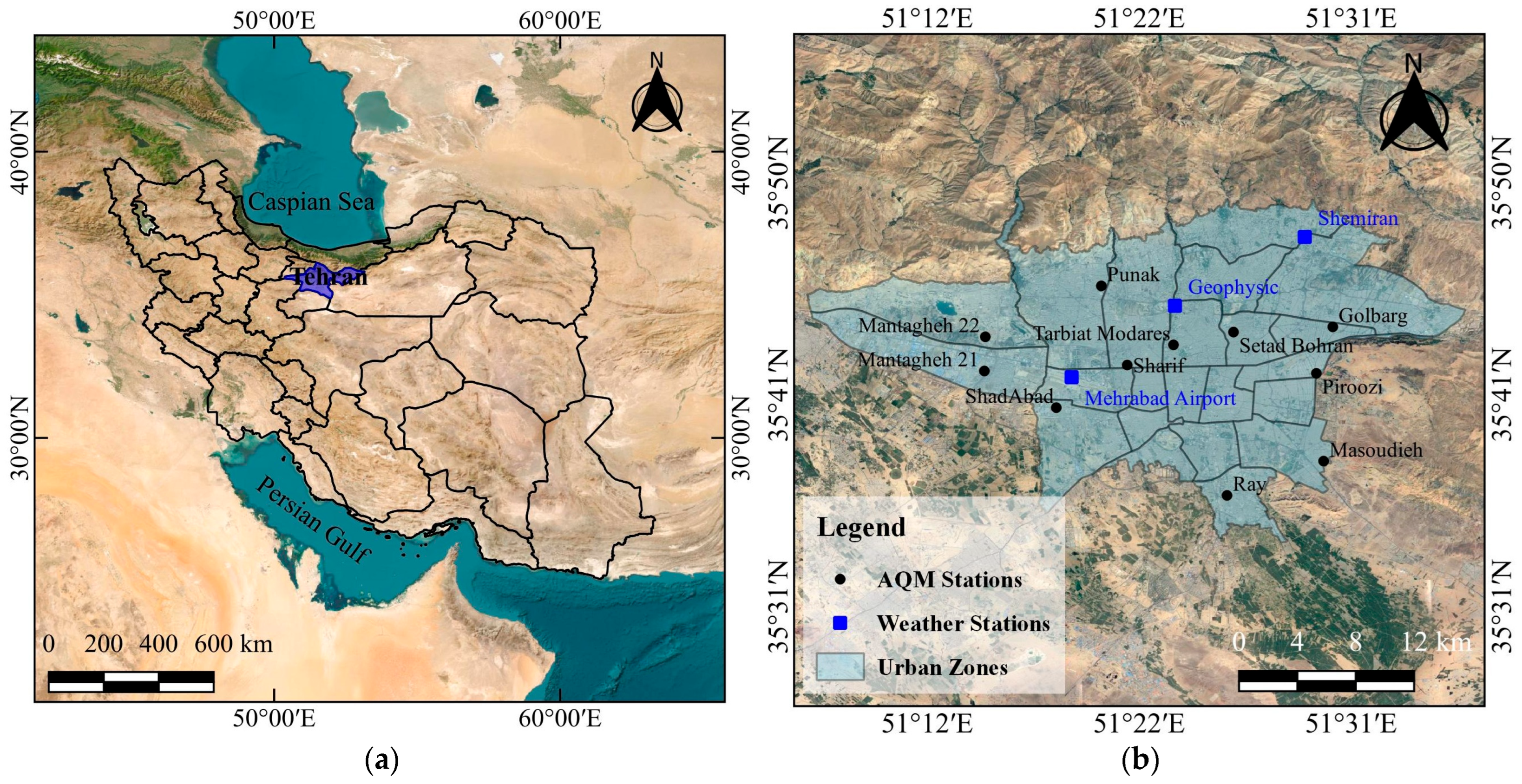
2.1. Study Area and Data Description
2.2. Data Preprocessing
2.3. Problem Formulation
3. Theoretical Background
3.1. GCNs
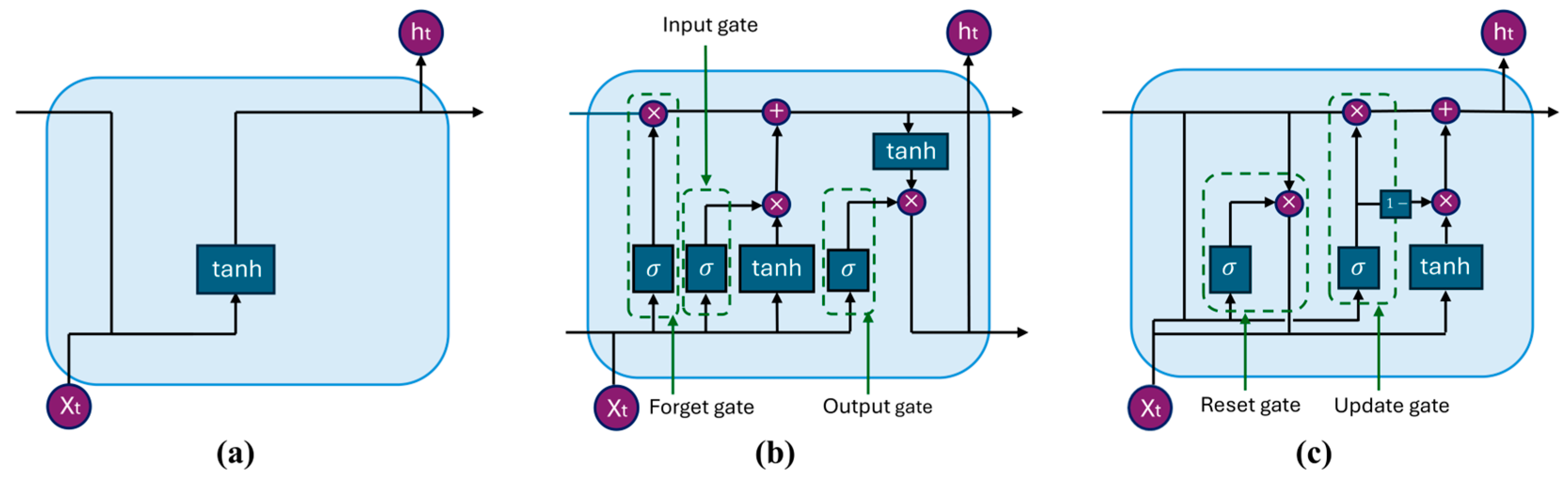
3.2. RNNs
4. Proposed Model and Experimental Settings
4.1. Model Design
4.1.1. Copula-Based Dependency Analysis Block
4.1.2. Pollutant Time Series Clustering Block
4.1.3. Graph Convolution Block
4.1.4. GRU Block
4.1.5. Output Block
4.2. Model Validation
4.3. Model Evaluation
- (1)
- GRU competitive method
- (2)
- LSTM competitive method
- (3)
- GRU and LSTM with multi-head attention competitive method
- (4)
- CNN-GRU competitive method
- (5)
- Distance-based GCN-GRU and wind-driven dynamic GAT-GRU
4.4. Experimental Settings
5. Results
5.1. PM2.5 Dependency on Other Pollutants
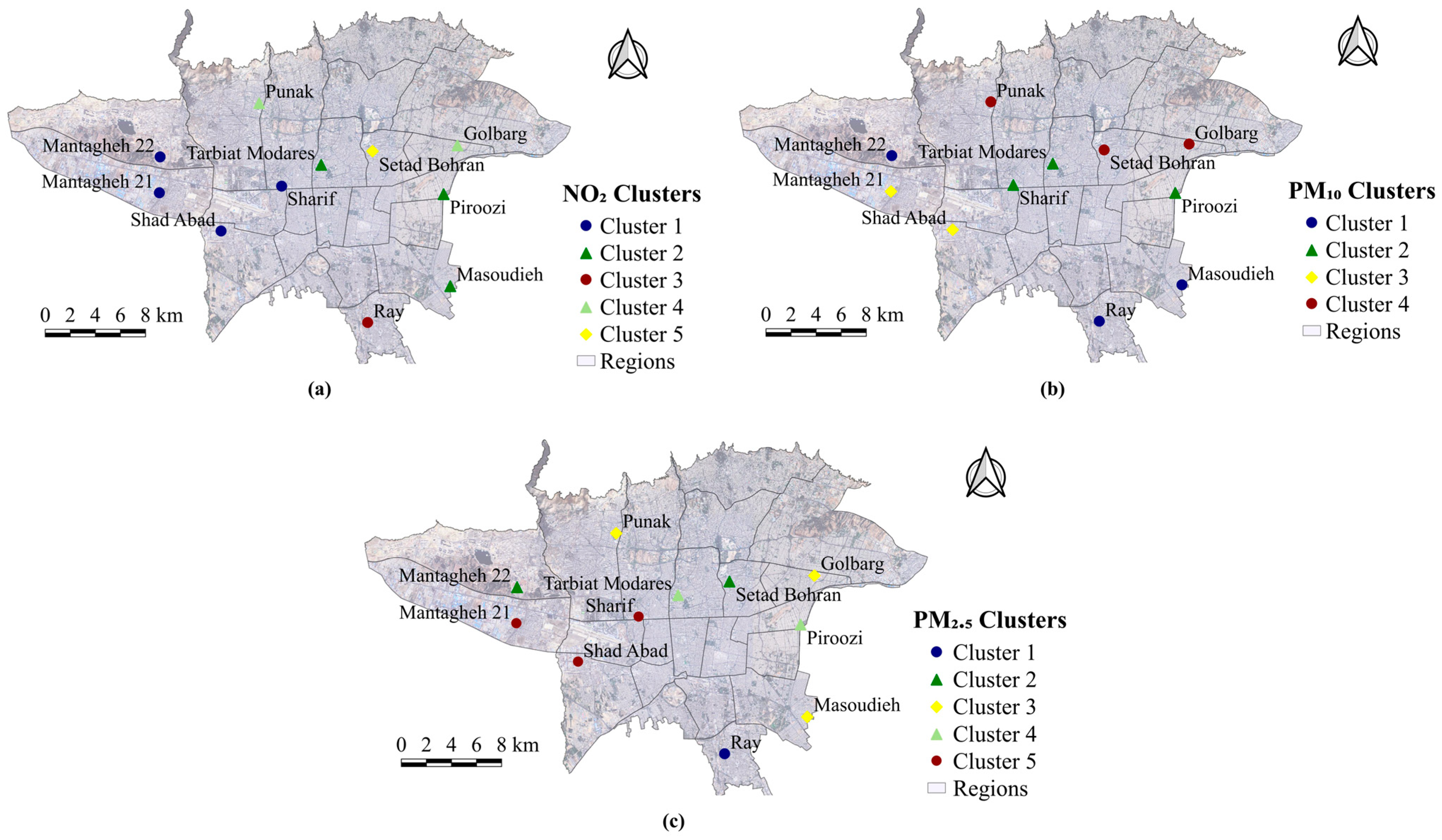
5.2. Spatial Clustering of AQMSs
5.3. Comparison of Model Performance Across Spatial Clustering of AQMSs
5.4. Comparison Results of Model Complexity
6. Discussion
7. Conclusions
Supplementary Materials
Author Contributions
Funding
Data Availability Statement
Conflicts of Interest
References
- Zhang, J.; Fu, M.; Wang, L.; Liang, Y.; Tang, F.; Li, S.; Wu, C. Impact of Urban Shrinkage on Pollution Reduction and Carbon Mitigation Synergy: Spatial Heterogeneity and Interaction Effects in Chinese Cities. Land 2025, 14, 537. [Google Scholar] [CrossRef]
- WHO World Health Organization. Available online: https://www.who.int/news-room/fact-sheets/detail/ambient-(outdoor)-air-quality-and-health (accessed on 31 July 2025).
- Habibi, R.; Alesheikh, A.A.; Mohammadinia, A.; Sharif, M. An Assessment of Spatial Pattern Characterization of Air Pollution: A Case Study of CO and PM2. 5 in Tehran, Iran. ISPRS Int. J. Geo-Inf. 2017, 6, 270. [Google Scholar] [CrossRef]
- Liu, F.; Jia, S.; Ma, L.; Lu, S. Spatiotemporal Dynamic Evolution of PM2. 5 Exposure from Land Use Changes: A Case Study of Gansu Province, China. Land 2025, 14, 795. [Google Scholar] [CrossRef]
- Song, Y.; Mao, H.; Li, H. Spatio-Temporal Modeling for Air Quality Prediction Based on Spectral Graph Convolutional Network and Attention Mechanism. In Proceedings of the 2022 International Joint Conference on Neural Networks (IJCNN), Padua, Italy, 18–23 July 2022; IEEE: New York, NY, USA, 2022; pp. 1–9. [Google Scholar]
- Liu, Z.; Fang, Z.; Hu, Y. A Deep Learning-Based Hybrid Method for PM2. 5 Prediction in Central and Western China. Sci. Rep. 2025, 15, 10080. [Google Scholar]
- Guan, Q.; Wang, J.; Ren, S.; Gao, H.; Liang, Z.; Wang, J.; Yao, Y. Predicting Short-Term PM2. 5 Concentrations at Fine Temporal Resolutions Using a Multi-Branch Temporal Graph Convolutional Neural Network. Int. J. Geogr. Inf. Sci. 2024, 38, 778–801. [Google Scholar] [CrossRef]
- Wang, Z.; Hu, K.; Wang, Z.; Yang, B.; Chen, Z. Impact of Urban Neighborhood Morphology on PM2. 5 Concentration Distribution at Different Scale Buffers. Land 2024, 14, 7. [Google Scholar] [CrossRef]
- Faridi, S.; Niazi, S.; Yousefian, F.; Azimi, F.; Pasalari, H.; Momeniha, F.; Mokammel, A.; Gholampour, A.; Hassanvand, M.S.; Naddafi, K. Spatial Homogeneity and Heterogeneity of Ambient Air Pollutants in Tehran. Sci. Total Environ. 2019, 697, 134123. [Google Scholar] [CrossRef]
- Mun, H.; Li, M.; Jung, J. Spatial-Temporal Characteristics and Influencing Factors of Particulate Matter: Geodetector Approach. Land 2022, 11, 2336. [Google Scholar] [CrossRef]
- Alharbi, B.H.; Alduwais, A.K.; Alhudhodi, A.H. An Analysis of the Spatial Distribution of O3 and Its Precursors during Summer in the Urban Atmosphere of Riyadh, Saudi Arabia. Atmos. Pollut. Res. 2017, 8, 861–872. [Google Scholar] [CrossRef]
- Hu, Y.; Li, Q.; Shi, X.; Yan, J.; Chen, Y. Domain Knowledge-Enhanced Multi-Spatial Multi-Temporal PM2. 5 Forecasting with Integrated Monitoring and Reanalysis Data. Environ. Int. 2024, 192, 108997. [Google Scholar] [CrossRef]
- Reichstein, M.; Camps-Valls, G.; Stevens, B.; Jung, M.; Denzler, J.; Carvalhais, N. Prabhat, fnm Deep Learning and Process Understanding for Data-Driven Earth System Science. Nature 2019, 566, 195–204. [Google Scholar] [CrossRef]
- Abbasi, M.T.; Alesheikh, A.A.; Lotfata, A.; Azizi, Z. Hybrid Graph Convolutional Networks for Air Quality Prediction: A Systematic Review of Foundations, Challenges, and Opportunities. Int. J. Environ. Sci. Technol. 2025. [Google Scholar] [CrossRef]
- Chen, Q.; Ding, R.; Mo, X.; Li, H.; Xie, L.; Yang, J. An Adaptive Adjacency Matrix-Based Graph Convolutional Recurrent Network for Air Quality Prediction. Sci. Rep. 2024, 14, 4408. [Google Scholar] [CrossRef]
- Hu, W.; Zhang, Z.; Zhang, S.; Chen, C.; Yuan, J.; Yao, J.; Zhao, S.; Guo, L. Learning Spatiotemporal Dependencies Using Adaptive Hierarchical Graph Convolutional Neural Network for Air Quality Prediction. J. Clean. Prod. 2024, 459, 142541. [Google Scholar] [CrossRef]
- Zeng, Q.; Cao, Y.; Fan, M.; Chen, L.; Zhu, H.; Wang, L.; Li, Y.; Liu, S. Fine Particulate Matter Concentration Prediction Based on Hybrid Convolutional Network with Aggregated Local and Global Spatiotemporal Information: A Case Study in Beijing and Chongqing. Atmos. Environ. 2024, 333, 120647. [Google Scholar] [CrossRef]
- Liu, H.; Han, Q.; Lu, D.; Sheng, J.; Sui, S.; Sun, H. Fine-Grained Graph Convolutional Network with Learning-Based Bi-Relational Graph for Spatiotemporal Forecasting. Expert Syst. Appl. 2025, 265, 125959. [Google Scholar] [CrossRef]
- Zhao, Q.; Liu, J.; Yang, X.; Qi, H.; Lian, J. Spatiotemporal PM2. 5 Forecasting via Dynamic Geographical Graph Neural Network. Environ. Model. Softw. 2025, 186, 106351. [Google Scholar] [CrossRef]
- Huang, Y.; Han, F.; Feng, Q. A Novel Model for Predicting PM2. 5 Concentrations Utilizing Graph Convolutional Networks and Transformer. IEEE Access 2025. [Google Scholar]
- Zeng, Q.; Zeng, H.; Fan, M.; Chen, L.; Tao, J.; Zhang, Y.; Zhu, H.; Liu, S.; Zhu, Y. Adaptive Graph-Generating Jump Network for Air Quality Prediction Based on Improved Graph Convolutional Network. Atmos. Pollut. Res. 2025, 16, 102488. [Google Scholar] [CrossRef]
- Wang, P.; Zhang, H.; Cheng, S.; Zhang, T.; Lu, F.; Wu, S. A Lightweight Spatiotemporal Graph Dilated Convolutional Network for Urban Sensor State Prediction. Sustain. Cities Soc. 2024, 101, 105105. [Google Scholar] [CrossRef]
- Zheng, Y.; Capra, L.; Wolfson, O.; Yang, H. Urban Computing: Concepts, Methodologies, and Applications. ACM Trans. Intell. Syst. Technol. 2014, 5, 1–55. [Google Scholar] [CrossRef]
- Van, N.H.; Van Thanh, P.; Tran, D.N.; Tran, D.-T. A New Model of Air Quality Prediction Using Lightweight Machine Learning. Int. J. Environ. Sci. Technol. 2023, 20, 2983–2994. [Google Scholar] [CrossRef]
- Abbasi, M.T.; Alesheikh, A.A.; Jafari, A.; Lotfata, A. Spatial and Temporal Patterns of Urban Air Pollution in Tehran with a Focus on PM2. 5 and Associated Pollutants. Sci. Rep. 2024, 14, 25150. [Google Scholar] [CrossRef] [PubMed]
- Kalankesh, L.R.; Khajavian, N.; Soori, H.; Vaziri, M.H.; Saeedi, R.; Hajighasemkhan, A. Association Metrological Factors with Covid-19 Mortality in Tehran, Iran (2020-2021). Int. J. Environ. Health Res. 2024, 34, 1725–1736. [Google Scholar] [CrossRef] [PubMed]
- Taksibi, F.; Khajehpour, H.; Saboohi, Y. On the Environmental Effectiveness Analysis of Energy Policies: A Case Study of Air Pollution in the Megacity of Tehran. Sci. Total Environ. 2020, 705, 135824. [Google Scholar] [CrossRef] [PubMed]
- Zhu, J.; Ge, Z.; Song, Z.; Gao, F. Review and Big Data Perspectives on Robust Data Mining Approaches for Industrial Process Modeling with Outliers and Missing Data. Annu. Rev. Control 2018, 46, 107–133. [Google Scholar] [CrossRef]
- Singh, D.; Singh, B. Feature Wise Normalization: An Effective Way of Normalizing Data. Pattern Recognit. 2022, 122, 108307. [Google Scholar] [CrossRef]
- Jiang, W.; Luo, J. Graph Neural Network for Traffic Forecasting: A Survey. Expert Syst. Appl. 2022, 207, 117921. [Google Scholar] [CrossRef]
- Zhou, J.; Cui, G.; Hu, S.; Zhang, Z.; Yang, C.; Liu, Z.; Wang, L.; Li, C.; Sun, M. Graph Neural Networks: A Review of Methods and Applications. AI open 2020, 1, 57–81. [Google Scholar] [CrossRef]
- Zhang, S.; Tong, H.; Xu, J.; Maciejewski, R. Graph Convolutional Networks: A Comprehensive Review. Comput. Soc. Networks 2019, 6, 1–23. [Google Scholar] [CrossRef]
- Wu, G.; Al-qaness, M.A.A.; Al-Alimi, D.; Dahou, A.; Abd Elaziz, M.; Ewees, A.A. Hyperspectral Image Classification Using Graph Convolutional Network: A Comprehensive Review. Expert Syst. Appl. 2024, 257, 125106. [Google Scholar] [CrossRef]
- Bruna, J.; Zaremba, W.; Szlam, A.; LeCun, Y. Spectral Networks and Locally Connected Networks on Graphs. arXiv 2013, arXiv:1312.6203. [Google Scholar]
- Henaff, M.; Bruna, J.; LeCun, Y. Deep Convolutional Networks on Graph-Structured Data. arXiv 2015, arXiv:1506.05163. [Google Scholar]
- Defferrard, M.; Bresson, X.; Vandergheynst, P. Convolutional Neural Networks on Graphs with Fast Localized Spectral Filtering. Adv. Neural Inf. Process. Syst. 2016, 29. [Google Scholar]
- Kipf, T.N.; Welling, M. Semi-Supervised Classification with Graph Convolutional Networks. arXiv 2016, arXiv:1609.02907. [Google Scholar]
- Shin, J.; Yeon, K.; Kim, S.; Sunwoo, M.; Han, M. Comparative Study of Markov Chain with Recurrent Neural Network for Short Term Velocity Prediction Implemented on an Embedded System. IEEE Access 2021, 9, 24755–24767. [Google Scholar] [CrossRef]
- Hopfield, J.J. Neural Networks and Physical Systems with Emergent Collective Computational Abilities. Proc. Natl. Acad. Sci. USA 1982, 79, 2554–2558. [Google Scholar] [CrossRef]
- Farmanifard, S.; Alesheikh, A.A.; Sharif, M. A Context-Aware Hybrid Deep Learning Model for the Prediction of Tropical Cyclone Trajectories. Expert Syst. Appl. 2023, 231, 120701. [Google Scholar] [CrossRef]
- Elman, J.L. Finding Structure in Time. Cogn. Sci. 1990, 14, 179–211. [Google Scholar] [CrossRef]
- Hamedi, H.; Alesheikh, A.A.; Panahi, M.; Lee, S. Landslide Susceptibility Mapping Using Deep Learning Models in Ardabil Province, Iran. Stoch. Environ. Res. Risk Assess. 2022, 36, 4287–4310. [Google Scholar] [CrossRef]
- Schmidhuber, J.; Hochreiter, S. Long Short-Term Memory. Neural Comput. 1997, 9, 1735–1780. [Google Scholar]
- Fan, J.; Li, R.; Zhao, M.; Pan, X. A BiLSTM-Based Hybrid Ensemble Approach for Forecasting Suspended Sediment Concentrations: Application to the Upper Yellow River. Land 2025, 14, 1199. [Google Scholar] [CrossRef]
- Hakim, W.L.; Nur, A.S.; Rezaie, F.; Panahi, M.; Lee, C.-W.; Lee, S. Convolutional Neural Network and Long Short-Term Memory Algorithms for Groundwater Potential Mapping in Anseong, South Korea. J. Hydrol. Reg. Stud. 2022, 39, 100990. [Google Scholar] [CrossRef]
- Cho, K.; Van Merriënboer, B.; Gulcehre, C.; Bahdanau, D.; Bougares, F.; Schwenk, H.; Bengio, Y. Learning Phrase Representations Using RNN Encoder-Decoder for Statistical Machine Translation. arXiv 2014, arXiv:1406.1078. [Google Scholar]
- Faraji, M.; Nadi, S.; Ghaffarpasand, O.; Homayoni, S.; Downey, K. An Integrated 3D CNN-GRU Deep Learning Method for Short-Term Prediction of PM2. 5 Concentration in Urban Environment. Sci. Total Environ. 2022, 834, 155324. [Google Scholar] [CrossRef] [PubMed]
- Li, M.; Yan, Y. Comparative Analysis of Machine-Learning Models for Soil Moisture Estimation Using High-Resolution Remote-Sensing Data. Land 2024, 13, 1331. [Google Scholar] [CrossRef]
- Xiong, B.; Tang, J.; Li, Y.; Zhou, P.; Zhang, S.; Zhang, X.; Dong, C.; Gooi, H.B. A Flow-Rate-Aware Data-Driven Model of Vanadium Redox Flow Battery Based on Gated Recurrent Unit Neural Network. J. Energy Storage 2023, 74, 109537. [Google Scholar] [CrossRef]
- Szramowiat-Sala, K.; Marczak-Grzesik, M.; Karczewski, M.; Kistler, M.; Giebl, A.K.; Styszko, K. Chemical Investigation of Polycyclic Aromatic Hydrocarbon Sources in an Urban Area with Complex Air Quality Challenges. Sci. Rep. 2025, 15, 6987. [Google Scholar] [CrossRef]
- Yang, L.; Wang, G.; Wang, Y.; Wang, Y.; Ma, Y.; Zhang, X. A Rapid Computational Method for Quantifying Inter-Regional Air Pollutant Transport Dynamics. Atmosphere 2025, 16, 163. [Google Scholar] [CrossRef]
- Joe, H. Dependence Modeling with Copulas; CRC Press: Boca Raton, FL, USA, 2014; ISBN 1466583223. [Google Scholar]
- Lyu, M.-Z.; Fei, Z.-J.; Feng, D.-C. Copula-Based Cloud Analysis for Seismic Fragility and Its Application to Nuclear Power Plant Structures. Eng. Struct. 2024, 305, 117754. [Google Scholar] [CrossRef]
- Pan, S.; Joe, H. Predicting Times to Event Based on Vine Copula Models. Comput. Stat. Data Anal. 2022, 175, 107546. [Google Scholar] [CrossRef]
- Zhang, J.; Li, Y.; Liu, C.; Wu, B.; Shi, K. A Study of Cross-Correlations between PM2. 5 and O3 Based on Copula and Multifractal Methods. Phys. A Stat. Mech. Its Appl. 2022, 589, 126651. [Google Scholar] [CrossRef]
- Zhang, Y. Dynamic Effect Analysis of Meteorological Conditions on Air Pollution: A Case Study from Beijing. Sci. Total Environ. 2019, 684, 178–185. [Google Scholar] [CrossRef] [PubMed]
- Qi, Y.; Li, Q.; Karimian, H.; Liu, D. A Hybrid Model for Spatiotemporal Forecasting of PM2. 5 Based on Graph Convolutional Neural Network and Long Short-Term Memory. Sci. Total Environ. 2019, 664, 1–10. [Google Scholar] [CrossRef]
- Zhou, H.; Zhang, F.; Du, Z.; Liu, R. A Theory-Guided Graph Networks Based PM2. 5 Forecasting Method. Environ. Pollut. 2022, 293, 118569. [Google Scholar] [CrossRef]
- Wang, H.; Zhang, L.; Wu, R.; Cen, Y. Spatio-Temporal Fusion of Meteorological Factors for Multi-Site PM2. 5 Prediction: A Deep Learning and Time-Variant Graph Approach. Environ. Res. 2023, 239, 117286. [Google Scholar] [CrossRef] [PubMed]
- Pillai, P.S.; Babu, S.S.; Moorthy, K.K. A Study of PM, PM10 and PM2. 5 Concentration at a Tropical Coastal Station. Atmos. Res. 2002, 61, 149–167. [Google Scholar] [CrossRef]
- Wang, P.; Guo, H.; Hu, J.; Kota, S.H.; Ying, Q.; Zhang, H. Responses of PM2. 5 and O3 Concentrations to Changes of Meteorology and Emissions in China. Sci. Total Environ. 2019, 662, 297–306. [Google Scholar] [CrossRef] [PubMed]
- Chuang, M.-T.; Chou, C.C.-K.; Lin, C.-Y.; Lee, J.-H.; Lin, W.-C.; Chen, Y.-Y.; Chang, C.-C.; Lee, C.-T.; Kong, S.S.-K.; Lin, T.-H. A Numerical Study of Reducing the Concentration of O3 and PM2. 5 Simultaneously in Taiwan. J. Environ. Manag. 2022, 318, 115614. [Google Scholar] [CrossRef]
- Nabavi, S.O.; Haimberger, L.; Abbasi, E. Assessing PM2. 5 Concentrations in Tehran, Iran, from Space Using MAIAC, Deep Blue, and Dark Target AOD and Machine Learning Algorithms. Atmos. Pollut. Res. 2019, 10, 889–903. [Google Scholar] [CrossRef]
- Zamani Joharestani, M.; Cao, C.; Ni, X.; Bashir, B.; Talebiesfandarani, S. PM2. 5 Prediction Based on Random Forest, XGBoost, and Deep Learning Using Multisource Remote Sensing Data. Atmosphere 2019, 10, 373. [Google Scholar] [CrossRef]


| Variable | Unit | Range | Mean | St. Dev. |
|---|---|---|---|---|
| PM2.5 | [0.167, 249.724] | 30.680 | 20.309 | |
| PM10 | [0.677, 697.977] | 76.780 | 46.340 | |
| SO2 | ppb | [0.051, 142.400] | 7.561 | 6.472 |
| NO2 | ppb | [0.565, 301.055] | 48.597 | 22.942 |
| O3 | ppb | [0.0680, 213.035] | 20.702 | 20.204 |
| CO | ppm | [0.0075, 15.7300] | 1.871 | 1.269 |
| Temperature | °C | [−7.631, 40.888] | 17.770 | 10.191 |
| Pressure | mbar | [956.452, 1037.462] | 1011.236 | 8.928 |
| Humidity | % | [2.479, 99.147] | 36.656 | 20.766 |
| Dew point temperature | °C | [−26.819, 24.372] | 0.061 | 5.308 |
| Wind_x | m/s | [−11.653, 7.269] | −0.874 | 1.408 |
| Wind_y | m/s | [−18.558, 9.383] | −0.188 | 1.936 |
| Copula Family | Tail Dependence | Symmetry | Type of Dependence Captured | Typical Use Case in Air Pollution |
|---|---|---|---|---|
| Clayton | Lower tail (strong) | Asymmetric | Captures stronger association in low extremes | Simultaneous decrease in pollutant concentrations |
| Gumbel | Upper tail (strong) | Asymmetric | Captures stronger association in high extremes | Joint increase in pollutants under severe pollution events |
| t-Student | Both tails (moderate/strong) | Symmetric | Models symmetric tail dependence | Extreme events with co-movements in both directions |
| Gaussian | None (only linear correlation) | Symmetric | Captures linear correlation but no tail dependence | Mild/moderate dependence under normal conditions |
| Frank | No tail dependence (moderate) | Symmetric | Captures moderate dependence across the whole range | Balanced and non-extreme pollutant interactions |
| Pollutant | Fitted Cupola Model | |||
|---|---|---|---|---|
| O3 | Rotated Gumbel 90° | −0.262 | 0 | 0 |
| CO | Frank | 0.386 | 0 | 0 |
| NO2 | t-Student | 0.424 | 0.136 | 0.136 |
| SO2 | t-Student | 0.388 | 0.189 | 0.189 |
| PM10 | t-Student | 0.665 | 0.229 | 0.229 |
| Model | Metric | +1 | +2 | +4 | +8 | +12 | +24 | +48 | +72 |
|---|---|---|---|---|---|---|---|---|---|
| GRU | IA | 0.886 | 0.835 | 0.761 | 0.708 | 0.647 | 0.606 | 0.543 | 0.513 |
| R2 | 0.688 | 0.585 | 0.463 | 0.360 | 0.319 | 0.277 | 0.229 | 0.202 | |
| MAE () | 6.761 | 7.912 | 9.187 | 10.121 | 10.432 | 10.655 | 10.976 | 11.175 | |
| RMSE () | 10.208 | 11.780 | 13.438 | 14.709 | 15.170 | 15.647 | 16.194 | 16.550 | |
| LSTM | IA | 0.868 | 0.812 | 0.737 | 0.662 | 0.629 | 0.578 | 0.527 | 0.504 |
| R2 | 6.911 | 8.008 | 9.186 | 10.072 | 10.337 | 10.652 | 10.935 | 11.044 | |
| MAE () | 10.548 | 12.050 | 13.542 | 14.684 | 15.140 | 15.593 | 16.012 | 16.251 | |
| RMSE () | 10.548 | 12.050 | 13.542 | 14.684 | 15.140 | 15.593 | 16.012 | 16.251 | |
| GRU with multi-head attention | IA | 0.892 | 0.835 | 0.756 | 0.689 | 0.657 | 0.604 | 0.519 | 0.480 |
| R2 | 0.691 | 0.581 | 0.456 | 0.355 | 0.322 | 0.270 | 0.189 | 0.142 | |
| MAE () | 6.688 | 7.893 | 9.287 | 10.370 | 10.611 | 10.814 | 11.383 | 11.703 | |
| RMSE () | 10.121 | 11.788 | 13.478 | 14.722 | 15.128 | 15.705 | 16.614 | 17.171 | |
| LSTM with multi-head attention | IA | 0.877 | 0.825 | 0.748 | 0.669 | 0.638 | 0.585 | 0.503 | 0.471 |
| R2 | 0.663 | 0.562 | 0.437 | 0.329 | 0.294 | 0.245 | 0.162 | 0.128 | |
| MAE () | 7.090 | 8.160 | 9.440 | 10.458 | 10.739 | 11.021 | 11.608 | 11.783 | |
| RMSE () | 10.569 | 12.052 | 13.697 | 14.983 | 15.389 | 15.922 | 16.847 | 17.255 | |
| CNN-GRU | IA | 0.914 | 0.863 | 0.811 | 0.748 | 0.735 | 0.674 | 0.585 | 0.549 |
| R2 | 0.740 | 0.627 | 0.546 | 0.451 | 0.434 | 0.359 | 0.247 | 0.200 | |
| MAE () | 6.376 | 7.778 | 8.822 | 9.783 | 9.909 | 10.257 | 11.018 | 11.359 | |
| RMSE () | 9.838 | 11.783 | 13.045 | 14.313 | 14.421 | 14.854 | 15.966 | 16.440 | |
| Distance-based GCN-GRU | IA | 0.921 | 0.876 | 0.811 | 0.766 | 0.743 | 0.720 | 0.614 | 0.592 |
| R2 | 0.748 | 0.644 | 0.554 | 0.466 | 0.431 | 0.386 | 0.239 | 0.224 | |
| MAE () | 6.185 | 7.396 | 8.476 | 9.258 | 9.593 | 9.880 | 10.992 | 11.089 | |
| RMSE () | 9.686 | 11.510 | 12.922 | 14.147 | 14.485 | 14.539 | 16.066 | 16.211 | |
| Wind-driven dynamic GAT-GRU | IA | 0.935 | 0.892 | 0.843 | 0.786 | 0.752 | 0.715 | 0.567 | 0.546 |
| R2 | 0.802 | 0.717 | 0.632 | 0.551 | 0.506 | 0.457 | 0.284 | 0.241 | |
| MAE () | 5.613 | 6.763 | 7.856 | 8.848 | 9.184 | 9.471 | 10.796 | 10.972 | |
| RMSE () | 8.485 | 10.306 | 11.790 | 12.999 | 13.515 | 13.721 | 15.625 | 16.059 | |
| ClusLite-STGCN-GRU | IA | 0.920 | 0.884 | 0.842 | 0.788 | 0.776 | 0.752 | 0.633 | 0.624 |
| R2 | 0.765 | 0.687 | 0.617 | 0.533 | 0.512 | 0.475 | 0.323 | 0.317 | |
| MAE () | 5.905 | 7.008 | 8.001 | 8.909 | 9.062 | 9.244 | 10.458 | 10.461 | |
| RMSE () | 9.373 | 10.797 | 11.981 | 13.212 | 13.400 | 13.450 | 15.148 | 15.210 |
| Model | FBP (s) | FP (ms) | Total Epoch Time (s) | Inference Memory Allocated (MB) | FLOPs | Number of Parameters |
|---|---|---|---|---|---|---|
| Distance-based GCN-GRU | 383.35 | 11.03 | 440.65 | 920.40 | 78,312,960 | 252,844 |
| Wind-driven dynamic GAT-GRU | 995.87 | 18.01 | 1089.40 | 4166.76 | 105,318,400 | 176,304 |
| ClusLite-STGCN-GRU | 337.27 | 3.66 | 373.41 | 720.09 | 16,549,904 | 257,288 |
| Authors | Publication | Study Period | Model | Evaluation Criteria |
|---|---|---|---|---|
| Nabavi et al. [63] | 2019 | 2011–2016 | Machine Learning (Random Forest) | MAE = Not mentioned. |
| Zamani Joharestani et al. [64] | 2019 | 2015–2018 | Machine Learning (XGBoost) | |
| Faraji et al. [47] | 2022 | 2016–2019 | Deep Learning (3D CNN-GRU) | |
| Ours | - | 2019–2022 | Deep Learning (ClusLite-STGCN-GRU) |
Disclaimer/Publisher’s Note: The statements, opinions and data contained in all publications are solely those of the individual author(s) and contributor(s) and not of MDPI and/or the editor(s). MDPI and/or the editor(s) disclaim responsibility for any injury to people or property resulting from any ideas, methods, instructions or products referred to in the content. |
© 2025 by the authors. Licensee MDPI, Basel, Switzerland. This article is an open access article distributed under the terms and conditions of the Creative Commons Attribution (CC BY) license (https://creativecommons.org/licenses/by/4.0/).
Share and Cite
Abbasi, M.T.; Alesheikh, A.A.; Rezaie, F. A Lightweight Spatiotemporal Graph Framework Leveraging Clustered Monitoring Networks and Copula-Based Pollutant Dependency for PM2.5 Forecasting. Land 2025, 14, 1589. https://doi.org/10.3390/land14081589
Abbasi MT, Alesheikh AA, Rezaie F. A Lightweight Spatiotemporal Graph Framework Leveraging Clustered Monitoring Networks and Copula-Based Pollutant Dependency for PM2.5 Forecasting. Land. 2025; 14(8):1589. https://doi.org/10.3390/land14081589
Chicago/Turabian StyleAbbasi, Mohammad Taghi, Ali Asghar Alesheikh, and Fatemeh Rezaie. 2025. "A Lightweight Spatiotemporal Graph Framework Leveraging Clustered Monitoring Networks and Copula-Based Pollutant Dependency for PM2.5 Forecasting" Land 14, no. 8: 1589. https://doi.org/10.3390/land14081589
APA StyleAbbasi, M. T., Alesheikh, A. A., & Rezaie, F. (2025). A Lightweight Spatiotemporal Graph Framework Leveraging Clustered Monitoring Networks and Copula-Based Pollutant Dependency for PM2.5 Forecasting. Land, 14(8), 1589. https://doi.org/10.3390/land14081589