Article

Multifactor Configurational Pathways Driving the Eco-Efficiency of Cultivated Land Utilization in China: A Dynamic Panel QCA

1
College of Agriculture, Guangxi University, Nanning 530004, China
2
Research Institute of Forestry Policy and Information, Chinese Academy of Forestry, Beijing 100091, China
*
Author to whom correspondence should be addressed.
These authors contributed equally to this work.
Land 2025, 14(8), 1549; https://doi.org/10.3390/land14081549
Submission received: 17 June 2025 / Revised: 16 July 2025 / Accepted: 24 July 2025 / Published: 28 July 2025
(This article belongs to the Section Land Use, Impact Assessment and Sustainability)

Abstract

Cultivated land is fundamental to agricultural production, and the eco-efficiency of cultivated land utilization is widely acknowledged as a crucial indicator for assessing rational land use. Accordingly, this study applies a Super-SBM model with undesirable outputs to evaluate the eco-efficiency of cultivated land utilization (ECLU) across 31 provinces in China utilizing provincial panel data from 2005 to 2023 and further employs dynamic fuzzy-set qualitative comparative analysis to investigate, across spatial and temporal dimensions, how government policy, agricultural technology, socioeconomic conditions, and natural conditions interact to achieve a high ECLU and to elucidate the diverse configurational pathways through which these factors converge to deliver a high ECLU. Our findings demonstrate that the ECLU originates from the joint influence of several factors, and no single factor alone can provide a high level of eco-efficiency. In particular, a high GDP per capita and strong government agricultural expenditure intensity are pivotal for achieving a high ECLU, whereas a low GDP per capita and weak government agricultural expenditure intensity are the core conditions associated with poor eco-efficiency outcomes. We identify three distinct driving pathways that foster a high ECLU: the Economy–Technology–Government Synergistic Pathway, Nature–Economy Dual-Driver Pathway, and Government-Supported Land–Economy Pathway. Between-configuration consistency (BECONS) exhibits no significant temporal effect; however, a constellation of external factors triggered a pronounced, collective reduction in configurational consistency from 2008 to 2014. Regional analysis reveals pronounced heterogeneity: Spatially, the Economy–Technology–Government Synergistic Pathway is concentrated in China’s central and eastern provinces, the Nature–Economy Dual-Driver Pathway clusters mainly in the central belt, and the Government-Supported Land–Economy Pathway predominates in the west.

1. Introduction

Cultivated land is essential for human life and societal advancement, providing the foundation for global food security [1,2]. The global population increase, along with urbanization-induced reduction in cultivated land, has significantly diminished the agricultural land base: since the 1960s, per-capita cropland area has decreased from 0.41 hectares to 0.21 hectares. With food consumption rising in parallel, food security has become an acute worldwide concern [3,4]. Since China’s Reform and Opening-up four decades ago, total grain output has risen sharply. Yet, rapid urbanization and industrialization have steadily eroded cropland, and high-input, intensive farming has aggravated environmental degradation. Against a backdrop of shrinking farmland and mounting ecological stress, the urgent task is to raise cultivated land-use efficiency and curb its environmental pollution while safeguarding food production [5,6].
Since the early 1990s, Schaltegger and Sturm have advanced the concept of eco-efficiency, framing it as the ratio of economic value added to environmental burden [7]. The World Business Council for Sustainable Development subsequently broadened the idea and promoted it as a key metric of sustainability [8]—one now widely applied across industry [9], agriculture [10], tourism [11], and other sectors. The eco-efficiency of cultivated land utilization (ECLU) represents a contextualized application of the eco-efficiency concept to cultivated land systems. It reflects the degree to which cultivated land is used rationally in agricultural production—measured by the capacity to maximize agricultural and grain output while minimizing resource inputs and environmental pollution [12].
Research into the ECLU now rests on a solid foundation, spanning indicator frameworks, measurement methods, spatiotemporal characteristics, and driving factors. Debate, however, persists over the choice of undesirable outputs: some studies consider only carbon emissions [13,14,15,16], while others focus exclusively on non-point-source pollution [8,17,18]. More recently, scholars have highlighted cultivated land’s role as a substantial carbon sink—and, accordingly, have begun to include carbon sequestration as a desirable output in their assessments [19]. With respect to measurement methods, researchers now favor Data Envelopment Analysis (DEA), Stochastic Frontier Analysis (SFA), and Slack-Based Measure (SBM) models [14,20,21]. Studies are conducted at multiple scales—national [22], provincial [23], and municipal [24]—to capture variation in eco-efficiency. To probe its spatiotemporal characteristics, scholars typically track evolutionary patterns with kernel-density estimation [25], spatial autocorrelation statistics, and the Theil index [26,27]. For driving factors, some scholars have applied the Tobit regression model to analyze the driving factors behind China’s ECLU, finding that natural conditions, agricultural production conditions, regional economic development, and the level of regional technological development are the principal sources of variation [28]. Fan et al. utilized a Tobit regression model to analyze the Yangtze River Delta and demonstrated that the ECLU is enhanced by increased urbanization and regional GDP per capita [15]. Yang et al. quantified the ECLU in the Yangtze River Delta from 2001 to 2018 and analyzed the factors that influenced its level using spatial econometric models. Their results show that stronger socioeconomic development levels and greater investment in agricultural science and technology significantly enhance this efficiency [29]. Ma applied a geographical and temporal weighted regression (GTWR) model to probe the determinants of ECLU across China’s principal grain-producing regions. The results indicate that higher economic development consistently elevates ECLU, whereas technical factors—such as agricultural machinery density—exert region-specific effects [30]. Lyu et al., using a spatial β-convergence model, analyzed the ECLU across provinces in the middle and lower Yangtze River basin and found that a higher urbanization level, higher economic development level, a more advanced agricultural science and technology level, a greater economic contribution of family agriculture, and stronger financial support for agriculture each significantly enhance ECLU [31]. Synthesizing the preceding literature demonstrates that the ECLU is a complex system shaped jointly by policy, natural, technological, and economic forces and, crucially, constitutes a configurational phenomenon shaped by the joint action of multiple factors. Previous work using Tobit and other linear regression models has typically examined only the “net effect” of each individual factor in isolation. Accordingly, we define the ECLU as a dynamic “input–desirable-output–undesirable-output” process. To remedy gaps in the literature, we center our analysis on cropland-specific drivers, treating land, labor force, irrigation, agricultural machinery, agricultural plastic film, pesticides, and fertilizer as input variables. Outputs span three dimensions—carbon sink, economic value, and social benefits—whereas agricultural carbon emissions and agricultural non-point-source pollution are designated as undesirable outputs. Using a Super-SBM model with undesirable outputs, we quantify the ECLU across 31 Chinese provinces for the period of 2005–2023. Where conventional, static Qualitative Comparative Analysis (QCA) overlooks the temporal dimension—and hence cannot completely resolve causal complexity. We introduce dynamic QCA, a strategy that explicitly tracks the inter-provincial dynamics of ECLU and illuminates how alternative configurational pathways unfold over time. At the empirical and practical level, this study addresses three key issues. First, we obtain a reliable picture of the ECLU by applying a Super-SBM model with undesirable outputs to provincial data for 2005–2023, thereby overcoming the inaccuracy and pollution-blindness of earlier metrics. Second, we investigate how multiple drivers act in concert: dynamic QCA reveals the configurational pathways that deliver a high ECLU, correcting the single-factor bias of previous work and delimiting three pathways—the Economy–Technology–Government Synergistic Pathway, the Nature–Economy Dual-Driver Pathway, and the Government-Supported Land–Economy Pathway. Third, we examine regional heterogeneity, evaluating the suitability of each pathway across eastern, central, and western China and thus providing an evidence base for region-specific agricultural policy.
This study makes three primary contributions. First, drawing on a provincial panel, we quantify the ECLU for every Chinese province and deploy dynamic QCA in place of conventional linear regressions, a switch that both curbs omitted-variable bias and eases the endogeneity concerns that beset parametric models. Second, where earlier work typically examines a single factor at a time, we mine nationwide panel data to unearth how bundles of factors act together. The configurational approach captures the interaction and synergy of factors and offers enhanced explanatory power for the “many paths to the same outcome” patterns observed in ECLU. Third, because conventional static QCA relies on cross-sectional data and therefore overlooks how configurations change through time, we plot the year-to-year consistency of five configurational solutions, mapping the dynamic evolution of multifactor pathways and addressing a key limitation of earlier cross-sectional studies.
The remainder of this paper is organized as follows. Section 2 reviews the theoretical background and establishes the theoretical framework. Section 3 details the research design, including the Super-SBM model with undesirable outputs, dynamic QCA, necessary-condition analysis, variable construction, and the study area and data sources. Section 4 presents the empirical results. Section 5 discusses these findings, outlines the study’s limitations, and proposes directions for future work. Section 6 synthesizes the main conclusions and highlights their theoretical and practical implications.

2. Theoretical Framework

Rooted in eco-efficiency theory [7], we define the ECLU as maximizing agricultural output—grain yield and economic value—while minimizing resource inputs and environmental pollution. Earlier analysis demonstrates that ECLU emerges from the interplay of natural conditions, socioeconomic development, agricultural technology, and government policy; their joint effects therefore warrant explicit consideration [15,28,29,30,31]. Guided by this insight and by data availability, we construct a theoretical framework based on four dimensions: natural conditions, socioeconomic level, agricultural technology level, and government support.
Natural conditions constitute the resource bedrock of ECLU. The Multiple Cropping Index quantifies land-use intensity: a high value signals more frequent use of each hectare, raising per-unit output but often at the cost of heavier pesticide and fertilizer applications and greater ecological stress [32]. In contrast, the area of cultivated land reflects the absolute scale of regional cropland; enlarging that area can boost total harvests, yet it may also drive up carbon emissions [33]. The two measures, therefore, complement and counterbalance one another: expanding cropland eases pressure on individual fields, whereas increasing the Multiple Cropping Index functions as an efficiency-enhancing tactic when land expansion is constrained.
Socioeconomic conditions capture the objective setting in which cultivated land is managed; in this study, we proxy this dimension with GDP per capita and the urbanization rate, two indicators widely used to characterize regional socioeconomic development [15,30,34,35]. A higher GDP per capita signals a stronger regional purchasing power and larger agricultural investment, both of which tend to raise ECLU [36]. The urbanization level, the share of urban in the total population, influences cropland use on two fronts: as rural workers migrate to cities, land consolidation facilitates large-scale farming, and the more urbanized a region becomes, the more likely it is to adopt advanced, green production technologies [37]. A rising GDP per capita supplies the capital for such green upgrades, while higher urbanization levels unlock scale efficiencies through labor migration and land transfer. Acting in concert, the two indicators can markedly enhance the ECLU.
Agricultural technology is the principal, immediate driver of advancements in the ECLU. Within our indicator set, the level of agricultural technology is proxied by investment in science and technology—measured as local government expenditure on research and development. Local government expenditure on research and development constitutes a substantial share of public R&D funding in China. In 2023, local fiscal spending on science and technology reached approximately CNY 802.27 billion, accounting for 66.9% of national science and technology expenditure and providing a reliable indicator of regional government investment in agricultural technology. Increased investment fosters more sustainable production practices and refined management regimes, thereby elevating ECLU [36]. Agricultural mechanization density, which quantifies the extent of mechanized operations, can likewise boost land-use efficiency and curtail resource waste; nonetheless, improper machinery use may counteract these benefits by raising carbon emissions [25].
Government support provides the institutional underpinning for green cultivation. Here, government support is quantified as the ratio of fiscal outlays on agriculture, forestry, and water to the total sown area of crops, a metric that assesses the strength of local public investment in agriculture [31]. A higher ratio signals greater capacity to upgrade rural infrastructure and offset farmers’ losses from implementing greener practices, thereby steering them toward low-carbon, resource-conserving land use. In our conceptual framework, natural conditions furnish the foundation, socioeconomic factors shape the external milieu, agricultural technology drives efficiency advances, and government support delivers institutional guidance. Together, these four dimensions enable a holistic appraisal of how variable combinations impact the ECLU, offering robust evidence to inform policy design, foster green changes, and enhance productivity.
The three driving pathways identified through the dynamic QCA are marked in Figure 1.

3. Research Design

3.1. Research Methodology

3.1.1. Super-SBM Model with Undesirable Outputs

The Data Envelopment Analysis model, first introduced by Charnes et al. [38], has become a standard tool for measuring resource-use efficiency [39,40]. When inputs are excessive or outputs inadequate, however, DEA can overestimate the efficiency of a decision-making unit, introducing measurement bias. In addition, the classical DEA framework equates efficiency with producing more output from fewer inputs [41]. Yet, cropland systems inevitably yield undesirable outputs—such as carbon dioxide emissions and non-point-source pollution—alongside grain and other valuable products. To address these limitations, Tone introduced a Slack-Based Measure model that explicitly incorporates undesirable outputs [42]. Its mathematical formulations are provided in Equations (1) and (2).
E C L U = min 1 1 m × i = 1 m S i X i 1 + 1 s 1 + s 2 × r = 1 s 1 S r g Y r g + k = 1 S 2 S k b Y k b
s . t X 0 = X × λ + S Y 0 g = Y g × λ S g Y 0 b = Y b × λ + S b S 0 , S g 0 , S b 0
In Equations (1) and (2), ECLU denotes the cultivated-land eco-efficiency for the given year. m is the number of input variables, S 1 the number of desirable outputs, and S 2 the number of undesirable outputs. Symbols S i , S r g , and S k b represent, respectively, the input slack, the desirable-output slack, and the undesirable-output slack. For clarity, in the SBM framework, the slack variables measure the gap between each decision-making unit (DMU) and the efficiency frontier. A positive input slack reflects redundant input that could be further reduced without lowering output, while a positive output slack indicates an output shortfall that could be increased with the existing inputs. When all slacks equal zero, the DMU is fully efficient [43]. Variables X i , Y r g , and Y k b correspond to the input variables, the desirable-output variables, and the undesirable-output variables, while λ denotes the intensity weight. Symbols S , S g , and S b give the input slack, desirable-output slack, and undesirable-output slack for the DMU. Values X 0 , Y 0 g , and Y 0 b are the DMU’s observed inputs, desirable outputs, and undesirable outputs, whereas X , Y g , and Y b are the target inputs, desirable outputs, and undesirable outputs required to reach the efficiency frontier. The efficiency score of standard SBM models is limited to 1, rendering it impossible to differentiate between units that are entirely efficient. Consequently, we utilize the Super-SBM formulation with undesirable outputs to assess ECLU [44]. Its mathematical formulations are provided in Equations (3) and (4).
E C L U = min 1 m × i = 1 m x ¯ X i 1 s 1 + s 2 × r = 1 s 1 S r g Y r g + k = 1 S 2 S k b Y k b
s . t x ¯ X × λ Y g ¯ = Y g × λ Y b ¯ = Y b × λ x ¯ X 0 , Y g ¯ Y 0 g , Y b ¯ Y 0 b , λ 0

3.1.2. Dynamic QCA

QCA is a qualitative method grounded in Boolean algebra that combines qualitative and quantitative approaches to examine how multiple variables configure to generate complex causal relationships [45]. Compared with conventional linear regression, the Boolean framework of QCA helps avoid omitted-variable bias and mitigates potential endogeneity [46]. Traditional static QCA, however, relies on cross-sectional data and therefore overlooks the temporal dimension of configurations, making it difficult to trace how multifactor pathways evolve over time [47,48]. Accordingly, we apply dynamic QCA to provincial panel data to uncover the multiple configurational pathways through which various factors shape China’s ECLU [47]. Specifically, we analyze China’s provincial ECLU panel in R Studio 4.4.2, generating three sets of results—between-configuration consistency (BECONS), within-configuration consistency (WICONS), and pooled consistency (POCONS). BECONS assesses cross-sectional sufficiency for each year, WICONS gauges the temporal stability of each case, and consistency-adjusted distances are then used to track how these consistencies vary across both time and cases.

3.1.3. Necessary Condition Analysis

Necessary Condition Analysis (NCA), introduced by Dul in 2016, is designed to detect and test whether “necessary but not sufficient” causal conditions are present in a given phenomenon [49]. NCA selects such conditions from a larger set of antecedents and quantifies the degree to which each is necessary. Here, we integrate NCA with QCA: we first apply NCA to test whether any necessary condition must be in place to achieve a high eco-efficiency of cultivated land utilization, and then use QCA to verify the robustness of the necessary conditions identified by NCA [50].

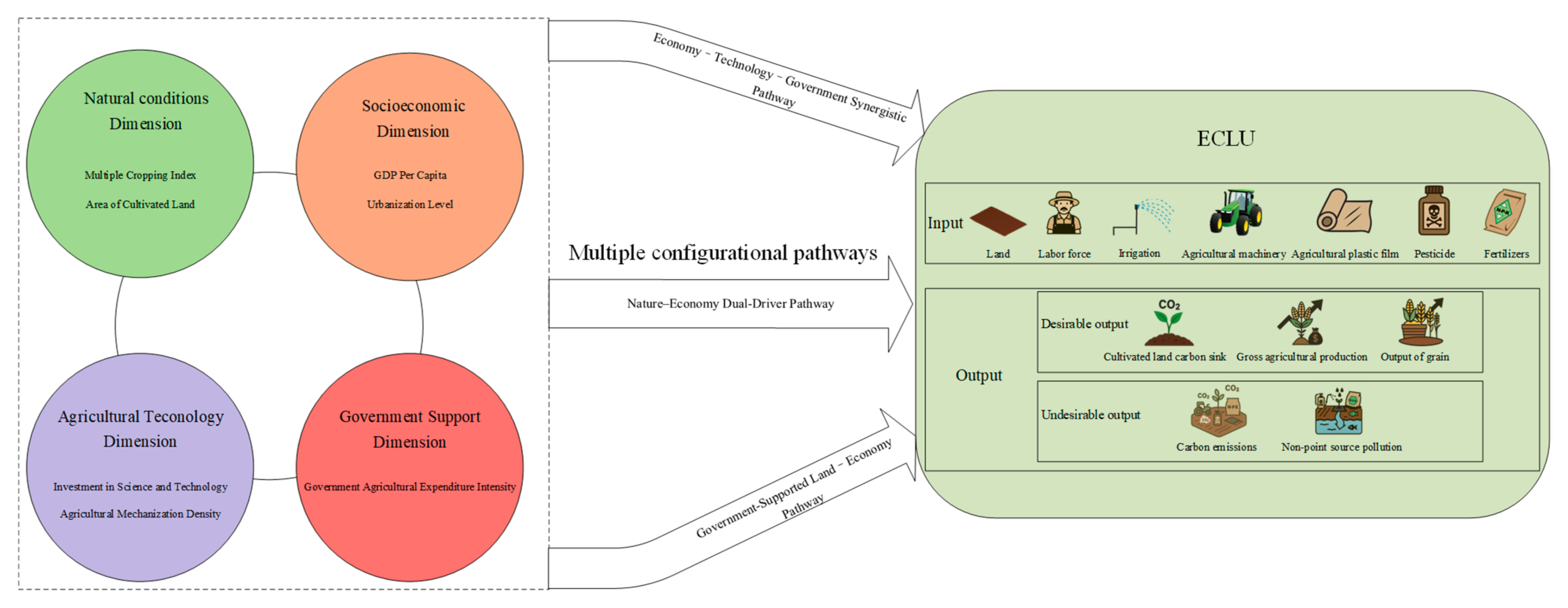
3.2. Index Selection

3.2.1. Outcome Variable

The outcome variable is the ECLU for 31 provinces, measured for 2005–2023 with a Super-SBM model that incorporates undesirable outputs. Because a high ECLU means producing more desirable output with fewer inputs and less undesirable output. Building on prior studies [8,18,19,29], we specify seven inputs—land, labor force, irrigation, agricultural machinery, agricultural plastic film, pesticide, and fertilizers. Agriculture functions both as a carbon sink and a carbon source, so the desirable outputs cover three dimensions: (1) a carbon sink quantified by agricultural carbon sequestration, (2) economic output represented by real gross agricultural production (base year 2005), and (3) social output represented by the output of grain. Undesirable outputs are the agricultural carbon emissions and agricultural non-point-source pollution generated in the production process. Detailed information is provided in Table 1.
Following Yin’s procedure, we estimate the number of agricultural workers by multiplying the crop farming output value as a proportion of the gross output value of agriculture, forestry, animal husbandry, and fishery by the number of agriculture, forestry, animal husbandry, and fishery employees [8]. Following Chen’s approach, we estimate total agricultural carbon sequestration using nine representative crops—rice, wheat, corn, millet, sorghum, beans, tubers, peanuts, rapeseed, cotton, sugarcane, sugar beet, vegetables, and tobacco leaf [51]. Its mathematical formulation is provided in Equation (5).
C * = k = 0 n C k D k = k = 0 n C k Y k H k
In Equation (5), C * is the carbon absorbed during the crop’s growth period; k denotes crop k ; D k is that crop’s biomass carbon content; C k is its carbon absorption rate; Y k is its economic yield; and H k is its economic coefficient. The economic coefficient—also called the harvest index—is defined as the ratio of harvested economic yield to the total above-ground dry biomass at maturity. Table 2 presents the carbon absorption rate, moisture content, and economic coefficient for the major crops [52].
Agricultural carbon emissions are calculated following Rong’s methodology [53]. Its mathematical formulation is provided in Equation (6).
E = E i = T i × δ i
In Equation (6), E denotes the total agricultural carbon emissions; Ei is the carbon emissions attributable to each carbon source; Ti represents the quantity of that carbon source; and δi is the corresponding carbon emission coefficient. Table 3 reports each carbon source, its coefficient, and the reference source.
Cultivated land non-point-source pollution is categorized as originating from two streams: solid agricultural residues and fertilizer discharge. The solid-residue stream is composed of straw or by-products from rice, wheat, corn, vegetables, peanuts, rapeseed, sunflower seeds, beans, and tubers, while fertilizer pollution is represented by phosphorus and nitrogen fertilizers. We estimate the provincial emissions of total nitrogen (TN), total phosphorus (TP), and chemical oxygen demand (COD) for China’s 31 provinces from 2005 to 2023 in accordance with Lai’s protocol [58,59,60]. Its mathematical formulation is provided in Equation (7).
P o l l u t i o n n m = γ P o n γ m × f a c t o r n γ 1 × f a c t o r n γ 2
In Equation (7), P o l l u t i o n n m denotes the cultivated land non-point-source pollution load for province n in year m. Symbol γ represents a pollution unit, and P o n γ m is the number of survey units for province n in year m. Parameter f a c t o r n γ 1 is the loss rate, whereas f a c t o r n γ 2 is the pollution production coefficient; both coefficients are taken from Lai [58,59]. Following the procedure of Cheng and Chang, the calculated emissions of TN, TP, and COD are converted into an equivalent standard pollutant load using benchmark concentrations of 0.2 mg/L, 1 mg/L, and 20 mg/L, respectively. This yields the total agricultural non-point-source pollution are expressed in units of 109 m3 [61].

3.2.2. Conditional Variable

Building on the foregoing discussion, we posit that ECLU is shaped by a constellation of drivers. Guided by both theory and data availability, we draw indicators from four dimensions—natural conditions, socioeconomic development, agricultural technology, and government support. The resulting panel comprises seven variables: Multiple Cropping Index (MCI) and area of cultivated land (ACL) for natural conditions; GDP per capita (GPC) and urbanization level (UL) for socioeconomic factors; investment in science and technology (STI) and agricultural mechanization density (AMD) for agricultural technology; and government agricultural expenditure intensity (GAEI) for government support. Detailed descriptions and reference sources are provided in Table 4.

3.3. Data Calibration
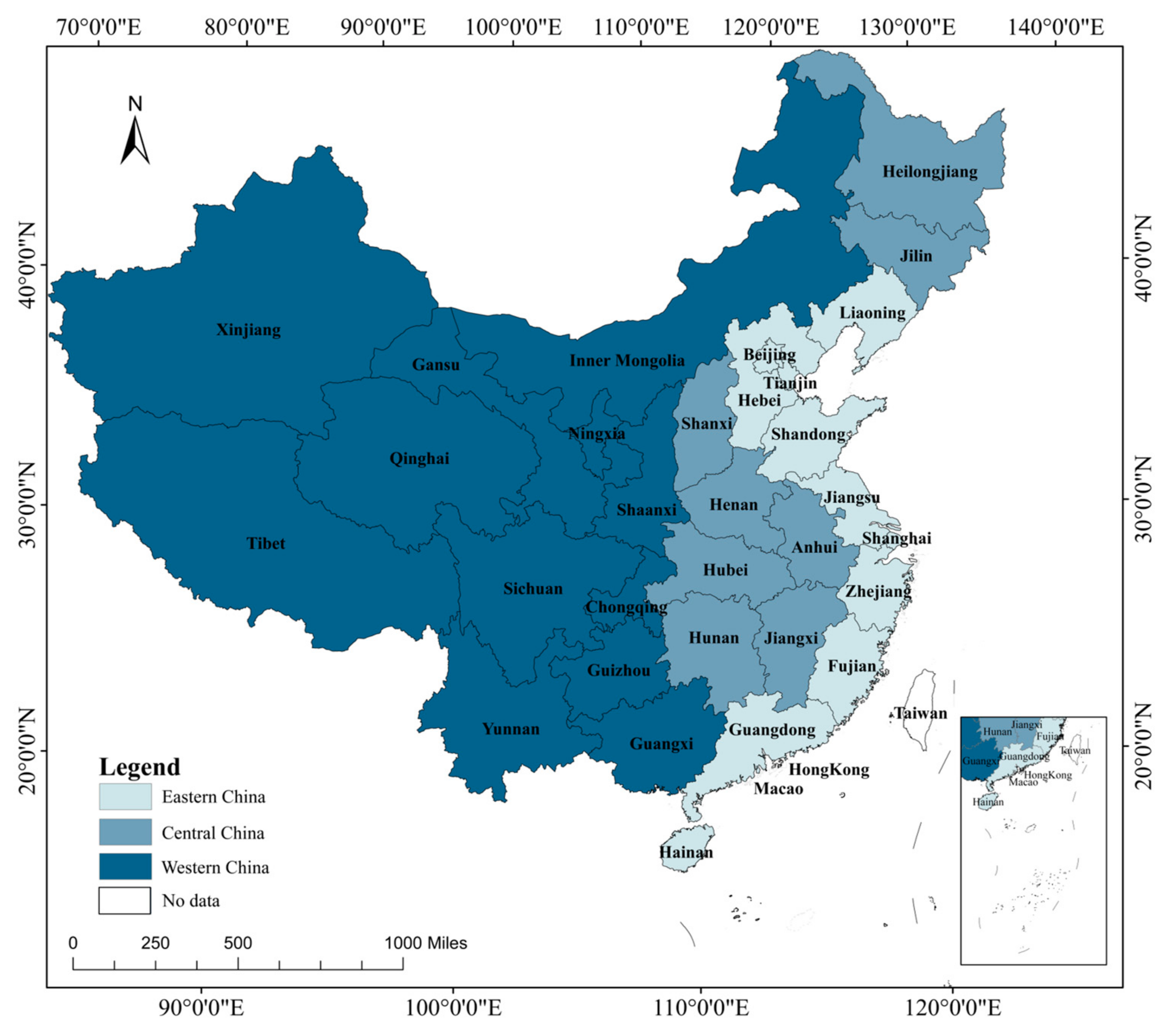
In QCA, data calibration converts raw values—guided by theory and empirical knowledge—into fuzzy-set memberships ranging from 0 to 1, providing the basis for subsequent analyses of consistency and coverage [62]. Using the direct calibration method [45], we set the 95%, 50%, and 5% quartiles as the calibration anchor points for full membership, the crossover point, and full non-membership, respectively. Because cases with a calibrated score of exactly 0.5 cannot enter the analysis, we follow Ragin’s guidance and recode any 0.5 value to 0.501 [63]. Table 5 summarizes the calibrated variables and their descriptive statistics.

3.4. Study Area

China, located in East Asia, has a vast territory of about 9.6 million km2, featuring a diverse topography and spanning multiple climatic zones. Administratively, the country comprises 34 provincial-level units (provinces, autonomous regions, and municipalities). Owing to data availability, our analysis focuses on the 31 mainland units for 2005–2023, excluding Hong Kong, Macao, and Taiwan. To compare regional differences in configurational coverage, we adopt the tripartite scheme of Xia et al. [64], grouping provinces into eastern, central, and western China. The eastern region comprises Beijing, Tianjin, Hebei, Liaoning, Shanghai, Jiangsu, Zhejiang, Fujian, Shandong, Guangdong, and Hainan; the central region comprises Shanxi, Jilin, Heilongjiang, Henan, Hubei, Hunan, Anhui, and Jiangxi; and the western region comprises Inner Mongolia, Chongqing, Sichuan, Guangxi, Guizhou, Yunnan, Shaanxi, Gansu, Qinghai, Ningxia, Xinjiang, and Tibet, as illustrated in Figure 2.

3.5. Data Source

We examine a cohort of 31 provinces in China (excluding Hong Kong, Macao, and Taiwan) from 2005 to 2023. The main sources of data are China’s Statistical Yearbook, the China Rural Statistical Yearbook, and the provincial annual statistical yearbooks. Linear interpolation is employed to cover any gaps. Gross agricultural production and GDP per capita are reported at constant 2005 prices to eliminate inflationary effects.

4. Results

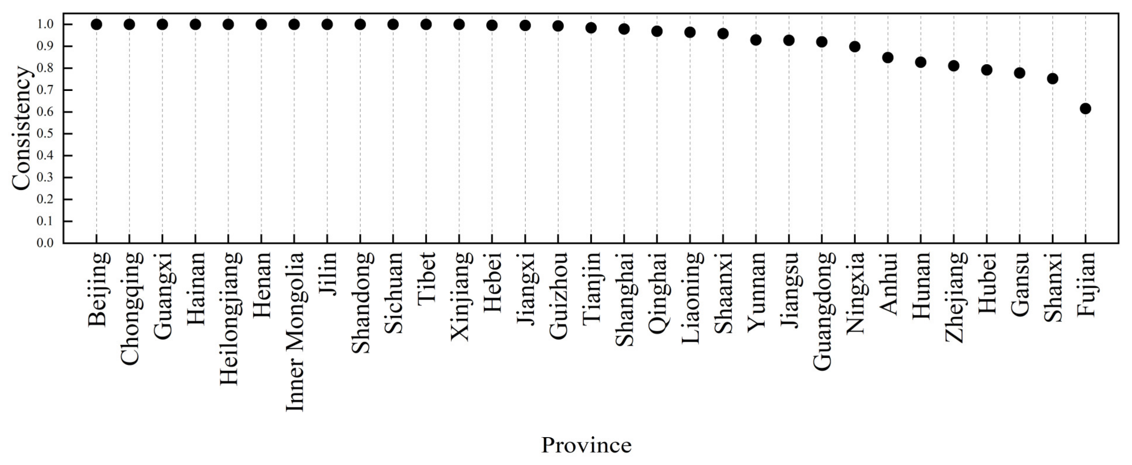
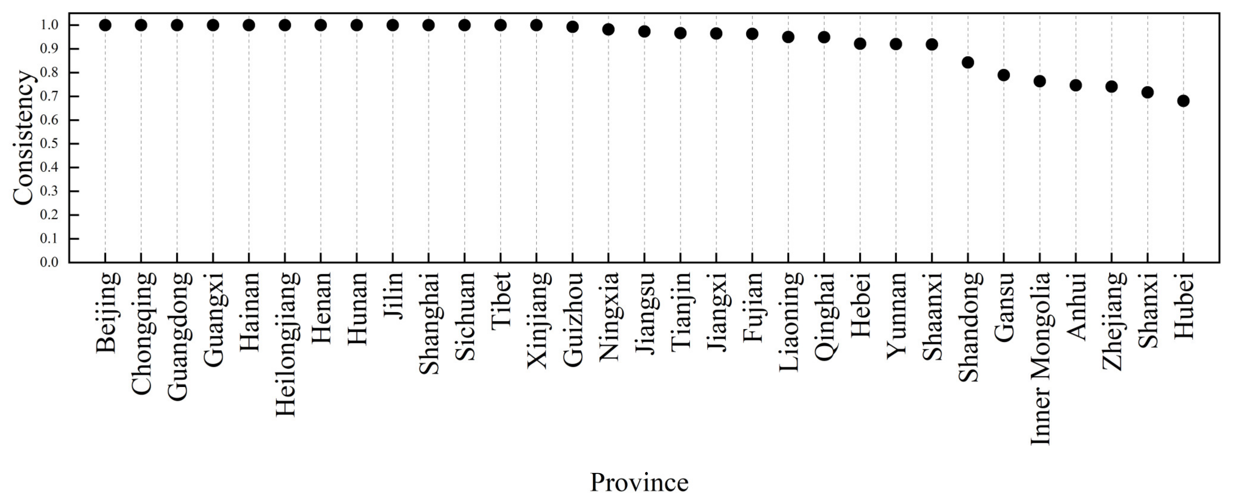
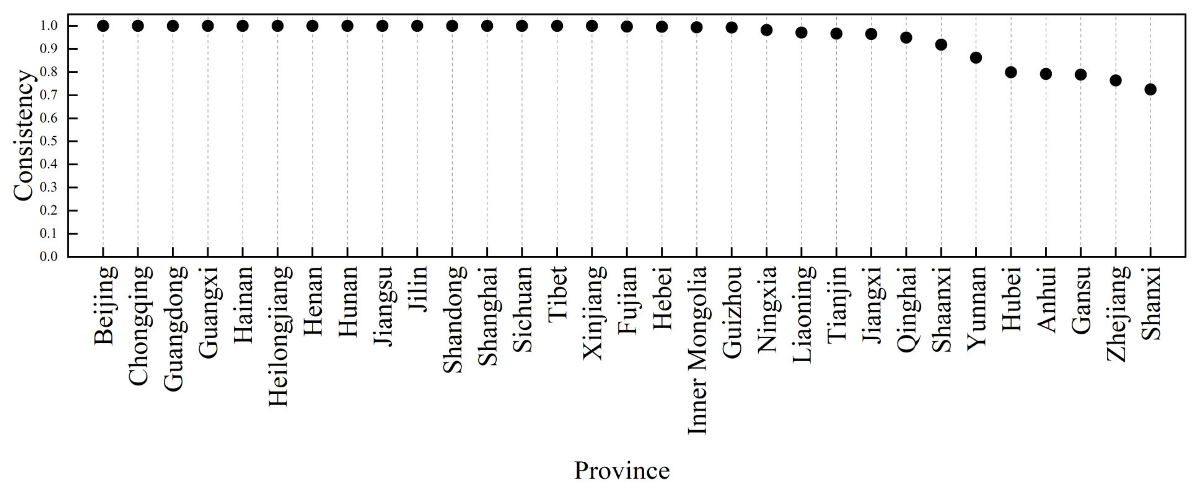
4.1. Necessity Analysis of Single Conditions

4.1.1. Necessity Analysis

Using the NCA package in R Studio 4.4.2, we applied both ceiling envelopment (CE) and ceiling regression (CR) to identify necessary conditions. For each of the seven candidate variables—MCI, ACL, GPC, UL, STI, AMD, and GAEI—the analysis generated the ceiling zone, effect size, c-accuracy, and p-value (Monte Carlo simulation substitution test); the results are summarized in the accompanying Table 6. In NCA, a variable is deemed necessary only when three stringent criteria are met simultaneously: effect size ≥ 0.1, p-value < 0.05, and c-accuracy > 95% [49,65,66,67]. Under both CE and CR, the p-values for MCI, ACL, GPC, UL, STI, and AMD all exceed 0.05, and their effect sizes remain below 0.1. GAEI attains statistical significance (p < 0.05) in both models, yet its effect size likewise falls short of the 0.1 threshold. Thus, none of the seven conditions satisfy NCA’s benchmark for necessity, indicating that no single factor alone qualifies as a necessary condition for achieving a high ECLU.
Building on the NCA results, a CR bottleneck analysis was performed to pinpoint the minimum levels each condition must meet to attain a specified outcome. As summarized in Table 7, attaining the ideal ECLU = 100% requires the following thresholds: MCI 17.6%, ACL 1.7%, GPC 67.9%, UL 63.7%, STI 1.5%, AMD 73.9%, and GAEI 61.5%. These figures confirm that a high ECLU depends on the joint contribution of several conditions, with GPC, UL, AMD, and GAEI emerging as the most demanding prerequisites. In Table 7, “NN” denotes “not necessary.”

4.1.2. Necessity Analysis of a Single Condition in QCA

Before undertaking the configurational analysis, each condition must be tested for necessity with respect to the outcome. As in conventional QCA, a condition is regarded as necessary if its POCONS is ≥0.90 and its pooled coverage (POCOV) exceeds 0.50 [68]. Because this study employs dynamic panel-data QCA, the test is tightened by an additional metric—the BECONS adjusted distance; a value < 0.20 indicates that the POCONS is sufficiently precise to support a claim of necessity [47]. Table 8 reports the consistency and coverage for all seven conditions. In every case, POCONS falls below the 0.90 threshold, signifying that no singular condition—whether associated with high or low eco-efficiency of cultivated land utilization—qualifies as a necessary factor.
Table S1 reveals 16 instances in which the BECONS adjusted distance exceeds 0.2, signaling a pronounced temporal effect; all corresponding causal configurations were re-examined and are collated in Table S1. Cases 1, 3, 4, 5, and 7 have BECONS < 0.90, ruling out necessity, whereas Cases 2, 8, 9, 10, 11, 12, 13, 14, and 15 show BECONS > 0.90 but between coverage (BECOV) < 0.50, likewise disqualifying them. Only Case 6 (2005) and Case 16 (2018) clear both thresholds; X–Y scatterplots drawn for these years reveal that Case 6 still fails the necessity test because observations cluster near the right-hand y-axis [69]. Although Case 16 satisfies both thresholds in 2018—between-consistency above 0.90 and between-coverage above 0.50—this pattern is observed in that single year only. Overall, a high level of GAEI does not constitute a necessary condition for a low ECLU. The scatterplot for Case 6 is shown in Figure 3, and the scatterplot for Case 16 is presented in Figure 4.

4.2. Configuration Analysis

Configuration analysis—the core of QCA—assesses how distinct combinations of conditions influence the outcome variable. Before conducting the analysis, three benchmark settings were adopted, drawing on earlier studies and the specifics of this dataset [68,70]: the consistency threshold was set at 0.80, the frequency threshold at 2, and the PRI consistency threshold at 0.65. These parameters retain 574 observational cases. No directional expectations were imposed during the counterfactual analyses. The procedure produces three solution sets—parsimonious, complex, and intermediate. The intermediate solutions serve as the principal results, while comparison with the parsimonious solutions identifies condition salience: any antecedent appearing in both sets is classified as a core condition, whereas one appearing only in the intermediate solutions is classified as a peripheral condition. The resulting configurations are summarized in Table 9.

4.3. Pooled Results Analysis

Table 9 shows an overall consistency of 0.901 for the high-ECLU configurations, well above the 0.80 sufficiency threshold, confirming that these configurations are sufficient for achieving a high ECLU [71]. The overall coverage is 0.507, meaning that, collectively, the configurations account for 50.7% of the high-ECLU cases in the dataset. The five configurations cluster into three thematic pathways. Configurations H1a and H1b make up the Economy–Technology–Government Synergistic Pathway; H2 stands for the Nature–Economy Dual-Driver Pathway; and H3a and H3b create the Government-Supported Land–Economy Pathway.
(1)
Economy–Technology–Government Synergistic Pathway. The configuration H1a demonstrates a consistency of 0.925 and a coverage of 0.391, indicating that 39.1% of the cases can be accounted for by this configuration. Its core conditions are a high GPC, high STI, low AMD, and high GAEI, with a high UL serving as a peripheral condition. This combination is sufficient to attain a high ECLU. The configuration H1b explains 24% of the cases, as it achieves a consistency of 0.942 and a coverage of 0.240. Although it shares the same core conditions—high GPC, high STI, low AMD, and high GAEI—it relies on a high MCI and high ACL as peripheral conditions to achieve a high ECLU. Thus, both configurations have identical cores, while their peripheral conditions are substitutable. Financial and technological resources can compensate for lower mechanization density or limited natural endowments in provinces with a strong economic capacity, active agricultural innovation, and robust policy support. This enables precise and efficient resource allocation and, ultimately, a high ECLU. Regions with higher levels of economic development typically command greater advantages in the allocation of agricultural inputs, enabling them to raise the ECLU [72]. Shanghai illustrates this dynamic. As China’s economic center, Shanghai leverages its robust economic strength to keep upgrading agricultural production conditions and thus consistently raise ECLU. In 2021, Shanghai’s contribution rate of agricultural scientific and technological progress reached 79.09%, among the highest nationwide, and the city consistently ranks near the top in agricultural modernization and indigenous innovation capacity [73]. Policy support reinforces these strengths. In 2025, the municipal government issued the Implementation Opinions on Accelerating Agricultural Science-and-Technology Innovation, calling for an integrated innovation system that links universities, research institutes, and enterprises to boost in-house R&D and speed up the commercialization of research outputs. A 2024 notice—On the Allocation of Funds for Cultivated Land Fertility Protection Subsidies—directs government subsidies to soil fertility protection, promoting pollution abatement and carbon mitigation in cultivated land use and further enhancing the city’s ECLU.
(2)
Nature–Economy Dual-Driver Pathway. Configuration H2 obtains a consistency of 0.911 and a coverage of 0.299, indicating that 29.9% of the cases can be accounted for by this configuration. Its core conditions are a high ACL, high GPC, low MCI, and low AMD; a high UL and low STI serve as peripheral conditions. In practice, where natural constraints keep both re-cropping intensity and mechanization modest, expanding the scope of cultivated land operations, combined with strong economic resources, can offset limited technological input and still deliver a high ECLU. Inner Mongolia exemplifies this pathway. Owing to its climate, the region produces only one crop per year, yielding a low MCI. Yet, in 2023, its cultivated land endowment reached 11,466.7 kha—about 10% of China’s total and second only to Heilongjiang. In 2024, GPC stood at CNY 110,011, eighth nationwide and among the highest in China’s central–western region. Prior work contends that favorable economic conditions reinforce farmers’ ecological awareness and encourage conservation tillage, allowing land abundance to translate into a high ECLU despite technological limitations [74].
(3)
Government-Supported Land–Economy Pathway. Configuration H3a records a consistency of 0.926 and a coverage of 0.281, indicating that 28.1% of the cases can be accounted for by this configuration. Its core conditions are a high ACL, high GPC, high GAEI, and low MCI and STI; a high UL serves as a peripheral condition. Together, these features are sufficient to achieve a high ECLU. Configuration H3b achieves a consistency of 0.940 and a coverage of 0.267, accounting for 26.7% of the cases. It shares the same core conditions as H3a—high ACL, high GPC, high GAEI, and sub-threshold MCI and STI—and adds a low AMD. Thus, the two configurations possess identical cores and substitute each other in their peripheral requirements. Xinjiang exemplifies this pathway. The region’s contribution rate of agricultural scientific and technological progress has long lagged behind the national average [75], and its harsh inland climate limits multiple cropping, yielding a low MCI. Yet, Xinjiang commands vast cultivated land—about 7066.7 kha, or 5.5% of China’s total—and strong fiscal support: in 2024, budgetary expenditure on agriculture, forestry, and water affairs reached CNY 98.63 billion, up 22.6% year-on-year. By leveraging extensive land resources, a robust economic capacity, and vigorous government funding, Xinjiang compensates for technological and natural constraints and achieves a higher ECLU.

4.4. Between Results

Figure 5 plots the temporal trajectory of BECONS for the five configurations, addressing a limitation of earlier cross-sectional QCA studies. In every year, each configuration’s BECONS exceeds the sufficiency benchmark of 0.75, and all BECONS-adjusted distances remain below 0.20, indicating no discernible time effect. A closer look at configuration dynamics shows that all configurations maintained BECONS values between 0.8 and 1.0 over 2005–2023 but dipped notably during 2008–2014. One likely reason is the policy response to the 2008 global financial crisis: to spur domestic demand, the government introduced the 2009 Agricultural Machinery Purchase Subsidy Programme, releasing an initial CNY 10 billion. Rapid mechanization in most provinces thereafter weakened the explanatory power of the low-AMD condition in several configurations. Secondly, the MCI began to decline around 2009. The drop was likely triggered by grain price policies—such as minimum purchase prices for rice and wheat and a temporary corn stockpiling scheme—whose initial floor prices were relatively low and whose incentives reached farmers only after a lag. At the same time, rising input costs prompted many farmers to leave fields fallow seasonally or even for an entire year while taking up off-farm work [76]. These shifts increased uncertainty in production patterns and, in turn, weakened configurational consistency. Over the same period, an extreme drought swept northern China, affecting many provinces north of the Yangtze River and ranking as the worst event in half a century for some of them [77]. After 2009, a once-in-a-century drought struck the southwest, curbing crop yields and inflicting substantial economic losses [78]. To offset these shocks, farmers expanded irrigation and intensified pesticide and fertilizer use—practices that, when applied in excess, undermine the ECLU. The combined impact of these shocks drove down the consistency of all five configurations. From 2014 onward, however, consistency rose significantly; after 2018, the BECONS values stabilized at about 1.0, and from 2021, they reached 1.0 across the board. This pattern indicates that, throughout 2005–2023, all five configurations retained a robust explanatory capacity and consistently proved sufficient for delivering a high ECLU.

4.5. Within Results

WICONS gauges how a configuration’s explanatory strength varies across provinces. Table 9 shows that the WICONS adjusted distance falls below 0.20 for all five high-ECLU configurations, indicating negligible regional heterogeneity; even so, each configuration maintains a consistency above 0.75 in most provinces. A single province can therefore achieve a high ECLU through several pathways. In Shanxi, for example, consistency for H3a is relatively low at 0.677, and yet it exceeds 0.70 in H1a, H1b, H2, and H3b. Fujian scores a relatively modest 0.615 under H1a, but the other four configurations yield much higher values, the highest reaching 0.997. These patterns underscore the versatility of the configurational solutions across China’s provincial landscape. The WICONS distribution plots for the five configurations are shown in Figure 6, Figure 7, Figure 8, Figure 9 and Figure 10: Figure 6 corresponds to H1a, Figure 7 to H1b, Figure 8 to H2, Figure 9 to H3a, and Figure 10 to H3b.
Coverage was stratified by eastern, central, and western China, and a regional configuration coverage mean was calculated for each zone. The Economy–Technology–Government Synergistic Pathway is responsible for the highest proportion of cases in the central region, followed by a lesser proportion in the east and the smallest proportion in the west, as illustrated in Table 10. Compared with western China, the central and eastern regions experience higher levels of economic development. Their accumulated economic advantages finance greater agricultural R&D and infrastructural investment, resulting in more advanced technology on the farm. In these wealthier areas, producers are more inclined to adopt conservation tillage and other green practices, and government support for agriculture is both larger and more stable. Together, strong economic capacity, technological progress, and sustained public funding form a mutually reinforcing driver that delivers a high ECLU. Typical provinces that follow this pathway include Shanghai, Fujian, Guangdong, and Jiangsu in the east; Jiangxi and Hubei in the center; and Chongqing and Sichuan in the west. The second pathway—the Nature–Economy Dual-Driver Pathway—covers the largest proportion of cases in the central region and, to a lesser extent, in the west. Its core conditions are a high ACL and GPC, with a high UL acting as a peripheral condition. The pathway therefore suits provinces that combine ample cultivated land with a solid but not necessarily advanced degree of urbanization, particularly in the central region and parts of the west. Heilongjiang exemplifies the pattern in the center, while Inner Mongolia is its leading representative in the west. The third pathway—the Government-Supported Land–Economy Pathway—is concentrated almost entirely in western China. Provinces in this zone share abundant cropland but operate under harsh natural and geographic constraints; they post a low MCI and only modest levels of agricultural technology. Xinjiang is the pathway’s most emblematic case.

4.6. Configurational Analysis of Low ECLU

Exploiting the causal asymmetry inherent in QCA, we also examined configurations that lead to a low ECLU. Table 9 reveals three such pathways, which fall into two categories on the basis of their core conditions: a Nature–Economy–Government Deficit Pathway and a Socioeconomic Deficit Pathway. Inspection of the pooled results indicates that a low GPC and low UL—markers of weak socioeconomic development and limited government agricultural support—are the primary drivers of poor ECLU performance.
The Nature–Economy–Government Deficit Pathway comprises configurations H4 and H6. Examination of H4 shows that a high AMD, together with a low MCI, low GPC and low GAEI, constitutes the core conditions. When coupled with a low ACL and low UL as peripheral conditions, this configuration yields a low ECLU. This finding suggests that when economic resources are constrained, government support is limited, and natural conditions restrict multiple cropping; increased mechanization cannot, on its own, raise ECLU. This configuration is observed mainly before 2014 in provinces such as Shanxi, Qinghai, Ningxia, and Gansu. Configuration H6 is marked by a low MCI, low GPC, low GAEI, and high AMD as its core conditions, with a low UL and low STI as peripheral conditions—a combination that yields a low ECLU. This configuration illustrates that where economic development lags, natural conditions are poor, and agricultural technology remains limited; even a high density of farm machinery alone cannot yield a high ECLU. Representative cases are found mainly in Gansu and Shanxi prior to 2014.
Configuration H5 embodies the Socioeconomic Deficit Pathway. As Table 9 shows, its core conditions are a high MCI, high ACL, high AMD, and low GPC, whereas a low UL and low GAEI act as peripheral conditions. The pathway is exemplified by Henan and Hebei, with most instances occurring before 2015.

4.7. Further Analysis

Inspection of the eight configurational pathways that give rise to either a high or low ECLU underscores the pivotal role played by socioeconomic development and government support. In all five high-ECLU pathways, a high GPC and high GAEI appear as core conditions, whereas in the three low-ECLU pathways, their counterparts—low GPC and low GAEI—constitute the core. A plausible explanation is that greater affluence gives farmers the financial latitude to adopt advanced technologies—energy-efficient machinery, drip irrigation and fertigation systems, and other precision-farming tools—thereby curbing excessive extraction of land and water resources and fostering more sustainable cropland use. This interpretation is consistent with prior findings in the literature [8,28,29,30]. Additionally, provinces with a high GAEI possess the fiscal capacity to upgrade public infrastructure—high-standard farmland, modern drainage and irrigation systems, and integrated water–fertilizer networks—thereby curbing pollution, boosting resource-use efficiency, and replacing traditional, ecology-neglecting modes of extensive cultivation [79]. Ample budgets also enable fiscal instruments such as ecological compensation schemes that encourage farmers to adopt low-carbon, low-pollution practices. In contrast, where both GPC and GAEI are weak, technological renewal lags behind and environmental investment remains scant, constraining any improvement in the ECLU. Regions that already combine a high GPC with strong government support for agriculture can pursue either of two pathways to attain a high ECLU: technological upgrading or large-scale cultivated-land operations.
Moreover, juxtaposing configurations H1a and H3a shows that, under the same preconditions of high GPC and strong GAEI, H1a attains a high ECLU through elevated STI, whereas H3a achieves the same outcome via an extensive ACL—implying that agricultural technology and land endowment function as substitutable routes to a high ECLU. When cultivated land is scarce, raising eco-efficiency depends on boosting the output per unit area. A high STI signals the widespread adoption of capital-intensive technologies—precision irrigation–fertigation systems, digital agriculture platforms, and the like. By coupling such technology-intensive production with precisely targeted inputs, farms can achieve high yields and low emissions on limited land. Where the STI is somewhat lagging, provinces with strong government support can reach the same goal by using fiscal subsidies to finance land transfers or leases, thereby enlarging the operational holding [80]. Scale economies then spread machinery depreciation and other inputs over more hectares, lifting the ECLU.

4.8. Robustness Test

To test robustness, we adopted the guideline that “a re-specification of QCA parameters that produces no substantive change in the solutions can be regarded as robust.” [81] Accordingly, the consistency threshold was raised from 0.80 to 0.90. The recalculated configurations summarized in Table 11 are identical to the originals, confirming the robustness of our findings under this stricter criterion.

5. Discussion

This study investigates how natural conditions, socioeconomic circumstances, agricultural technology, and government policy combine to shape ECLU in China’s 31 provinces from 2005 to 2023. Using a super-efficiency SBM model with undesirable outputs, together with dynamic QCA and NCA, we identify five configurations that are sufficient for a high ECLU and classify them into three overarching pathways. The findings reveal both complementarity and substitutability among factor combinations, expanding the field beyond the single-factor focus of conventional linear-regression studies.
The Economy–Technology–Government Synergistic Pathway proposed in this study highlights that elevated socioeconomic development, substantial technological investment, and vigorous government support jointly drive improvements in ECLU, a finding that aligns closely with previous research. For example, Yang et al. reported that higher levels of socioeconomic development and greater investment in agricultural technology significantly enhance ECLU [29], while Lyu demonstrated that economic development, agricultural technology, and the intensity of fiscal support for agriculture all exert positive effects on ECLU [31]. Our findings further demonstrate that robust socioeconomic development, ample agricultural technological investment, and strong governmental support can yield a high ECLU even when natural conditions are restrictive. The second pathway—the Nature–Economy Dual-Driver Pathway—shows that when natural constraints depress both the MCI and the level of AMD, a high ECLU can still be achieved by enlarging operational land holdings and injecting greater economic resources, thereby offsetting limitations in agricultural technology. This result corroborates Zhou and Fan’s findings that a higher GPC and larger operational land holdings exert a positive influence on ECLU [15,82]. The third pathway—the Government-Supported Land-Economy Pathway—shows that a large ACL, high GPC, and strong GAEI together suffice to deliver a high ECLU. This result is consistent with earlier work emphasizing the efficacy of fiscal support [31].
A further comparison shows that GPC and GAEI emerge as core conditions in all five configurations, underscoring the critical role of both high GPC and strong government support in enhancing the ECLU. This finding is broadly consistent with earlier research [31,36]. In addition, whereas earlier work shows that either advanced agricultural technology or larger operational land holdings can improve the ECLU [19,29,36], this study finds that, once a high GPC and strong GAEI are in place, a clear substitution effect emerges between STI and ACL. Our configurational analysis therefore fills a gap left by previous studies.

Limitations and Future Work

Although this study adopts a dynamic configurational QCA framework to elucidate multiple pathways for improving the ECLU in China and contributes to the field, it nonetheless has several limitations. First, the indicator system employed to measure the ECLU requires further refinement to enhance its general applicability. Second, many variables—such as cultivated-land fragmentation, terrain, crop diversity, and off-farm employment—also affect the ECLU but could not be incorporated here owing to data constraints [35,83]. Third, limited data availability restricted the analysis to China’s 31 provinces. In this study, only two pairings—high GPC with high GAEI and low GPC with low GAEI—exceeded the required consistency threshold. The combinations of high GPC with low GAEI and low GPC with high GAEI did not meet the necessary consistency level, so they were left out, making it impossible to properly evaluate their effect on the ECLU. The provincial sample lacks enough cases to test these atypical pairings, and the same data constraints have thus far precluded a cross-national comparison.
Future studies could diversify data collection by incorporating social surveys and interviews. Remote-sensing imagery would make it possible to quantify geographic attributes such as cultivated-land fragmentation and terrain and to assess their effects on the ECLU. The configurational perspective could also be deployed at finer spatial scales—prefectural and county levels—or broadened to an international scope to compare the pathways that drive the ECLU across countries.

6. Conclusions

Drawing on China’s provincial panel data for 2005–2023, we first applied a Super-SBM model with undesirable outputs to estimate the ECLU in 31 provinces and treated this metric as the outcome variable. We then employed dynamic QCA to identify the configurational pathways through which multiple factors combine to deliver a high ECLU. The principal findings are as follows: (1) The combined NCA–QCA necessity analysis shows that no single factor is indispensable for achieving a high ECLU. Every high-ECLU configuration includes both a high GPC and strong GAEI, whereas a low GPC together with weak government support serve as the core factors underpinning a low ECLU. (2) Configurational analysis identifies three distinct forms that are sufficient for attaining a high ECLU: the Economy–Technology–Government Synergistic Pathway, the Nature–Economy Dual-Driver Pathway, and the Government-Supported Land–Economy Pathway. (3) Given a high GPC and strong GAEI, an advanced level of agricultural technology and an extensive cultivated-land area act as mutually substitutable conditions. (4) BECONS shows no clear temporal effect; however, all pathways experienced a marked, simultaneous decline during 2008–2014. This downturn was probably driven by the combined influence of the global financial crisis, policy shifts, and severe natural disasters, which temporarily weakened the explanatory power of each configuration. (5) Comparison of the regional configuration coverage means shows clear spatial preferences: cases captured by the Economy–Technology–Government Synergistic Pathway are concentrated in central and eastern China; those explained by the Nature–Economy Dual-Driver Pathway lie predominantly in the central region; and cases associated with the Government-Supported Land–Economy Pathway are found chiefly in the west. The third pathway—the Government-Supported Land-Economy Pathway—shows that a large ACL, high GPC, and strong GAEI together suffice to deliver a high ECLU. This result is consistent with earlier work emphasizing the efficacy of fiscal support.

6.1. Theoretical Implications

This study moves beyond previous research that focused exclusively on the “net effects” of individual factors and overlooked their interrelationships. We systematically investigate the interactive effects of seven variables drawn from four dimensions—natural conditions, socioeconomic development, agricultural technology, and government support—on the ECLU by adopting a configurational approach and building on the existing literature. Our analysis identifies five distinct pathways that improve ECLU, thereby addressing a significant limitation of conventional linear-regression methods that are unable to account for the combinational effects of multiple factors. As a result, this research broadens the scope of ECLU research from a single-factor perspective to a more intricate configurational framework. Our results provide a solid basis for creating policies and management plans that improve the ECLU, which helps make farming land resources more sustainable. Previous configurational analyses employing fuzzy-set Qualitative Comparative Analysis (fsQCA) typically relied on cross-sectional data, limiting their analytical scope to condition combinations and regional disparities at specific time points, without capturing dynamic, temporal trajectories. To overcome this limitation, our study innovatively integrates the temporal dimension into the configurational analysis of the ECLU, revealing dynamic evolutionary trends across various pathways. This provides methodological insights and theoretical implications for future research in this area.

6.2. Practical Implications

(1)
For provinces aligning with the Economy–Technology–Government Synergistic Pathway, governments should effectively allocate agricultural fiscal resources by providing subsidies to farmers adopting efficient and environmentally friendly production inputs and offering targeted incentives for precision agriculture and other advanced technologies. Resources should also be strategically channeled into research and development for ecological agricultural technologies. Additionally, fiscal subsidies could prioritize reducing chemical fertilizers, minimizing pesticide use, and enhancing soil remediation. Financial instruments, such as green agricultural bonds, may further accelerate the adoption of energy-efficient agricultural machinery. In regions characterized by fragmented farmland ownership, governments could facilitate land transfers to enable large-scale cultivation, with cooperatives or professional agricultural service providers delivering technical support and mechanized services.
(2)
For provinces characterized by the Nature–Economy Dual-Driver Pathway, governments should enhance fiscal investments in agriculture, particularly in farmland infrastructural improvements such as irrigation facilities, aiming to increase multiple-cropping indices and mechanization levels. Collaboration with local research institutes, universities, and technical colleges is also essential to deliver targeted farmer training, facilitate the dissemination of agricultural scientific knowledge, and provide tailored technological support. Moreover, the promotion of regionally appropriate green cultivation practices and strengthened investment in digital agricultural infrastructure should be prioritized to elevate local agricultural technological capacities.
(3)
In provinces explained by the Government-Supported Land–Economy Pathway, governments should increase technical subsidies targeted towards regions lagging in agricultural technology. Research institutes and universities should be encouraged to develop new crop varieties and technologies specifically suited to areas with low MCI, such as drought-resistant, high-yield cultivars and conservation tillage machinery. Fiscal subsidies can then accelerate adoption, phasing out outdated, energy-intensive equipment, thereby enhancing the mechanization density while reducing resource consumption and emissions.

Supplementary Materials

The following supporting information can be downloaded at: https://www.mdpi.com/article/10.3390/land14081549/s1.

Author Contributions

Conceptualization, Z.X., J.D. and Z.H.; Methodology, Z.X. and J.D.; Software, Z.X. and J.D.; Validation, C.Y. and Z.H.; Data Curation, C.Y.; Writing—Original Draft, Z.X. and J.D.; Writing—Review and Editing, L.Z.; Visualization, Z.X. and J.D.; Supervision, L.Z. and Z.H.; Project Administration, Z.H. All authors have read and agreed to the published version of the manuscript.

Funding

This research was funded by the National Natural Science Foundation of China (Grant No. 42477042).

Data Availability Statement

The raw data supporting the conclusions of this article will be made available by the authors on request.

Conflicts of Interest

The authors declare no conflicts of interest.

Abbreviations

Eco-efficiency of cultivated land utilization (ECLU); Data Envelopment Analysis (DEA); Stochastic Frontier Analysis (SFA); Slack-Based Measure (SBM); geographical and temporal weighted regression (GTWR); Qualitative Comparative Analysis (QCA); decision making unit (DMU); between-configuration consistency (BECONS); between coverage (BECOV); within-configuration consistency (WICONS); pooled consistency (POCONS); pooled coverage (POCOV); Necessary Condition Analysis (NCA); total nitrogen (TN); total phosphorus (TP); chemical oxygen demand (COD); Multiple Cropping Index (MCI); Area of Cultivated Land (ACL); GDP per Capita (GPC); Urbanization Level (UL); Investment in Science and Technology (STI); Agricultural Mechanization Density (AMD); Government Agricultural Expenditure Intensity (GAEI); ceiling envelopment (CE); ceiling regression (CR).

References

  1. Lambin, E.F.; Gibbs, H.K.; Ferreira, L.; Grau, R.; Mayaux, P.; Meyfroidt, P.; Morton, D.C.; Rudel, T.K.; Gasparri, I.; Munger, J. Estimating the World’s Potentially Available Cropland Using a Bottom-up Approach. Glob. Environ. Change 2013, 23, 892–901. [Google Scholar] [CrossRef]
  2. Su, M.; Guo, R.; Hong, W. Institutional Transition and Implementation Path for Cultivated Land Protection in Highly Urbanized Regions: A Case Study of Shenzhen, China. Land Use Policy 2019, 81, 493–501. [Google Scholar] [CrossRef]
  3. Li, X.; Zhao, L.; Chang, X.; Yu, J.; Song, X.; Zhang, L. Spatial and Temporal Evolution of the Eco-Efficiency of Cultivated Land Use in the Region around Beijing–Tianjin Based on the Super-EBM Model. Front. Ecol. Evol. 2023, 11, 1297570. [Google Scholar] [CrossRef]
  4. He, C.; Liu, Z.; Xu, M.; Ma, Q.; Dou, Y. Urban Expansion Brought Stress to Food Security in China: Evidence from Decreased Cropland Net Primary Productivity. Sci. Total Environ. 2017, 576, 660–670. [Google Scholar] [CrossRef]
  5. Liu, Y.; Zou, L.; Wang, Y. Spatial-Temporal Characteristics and Influencing Factors of Agricultural Eco-Efficiency in China in Recent 40 Years. Land Use Policy 2020, 97, 104794. [Google Scholar] [CrossRef]
  6. Cao, W.; Zhou, W.; Wu, T.; Wang, X.; Xu, J. Spatial-Temporal Characteristics of Cultivated Land Use Eco-Efficiency under Carbon Constraints and Its Relationship with Landscape Pattern Dynamics. Ecol. Indic. 2022, 141, 109140. [Google Scholar] [CrossRef]
  7. Schaltegger, S.; Sturm, A. Ökologische Rationalität: Ansatzpunkte Zur Ausgestaltung von Ökologieorientierten Managementinstrumenten. Die Unternehm. 1990, 44, 273–290. [Google Scholar]
  8. Yin, Y.; Hou, X.; Liu, J.; Zhou, X.; Zhang, D. Detection and Attribution of Changes in Cultivated Land Use Ecological Efficiency: A Case Study on Yangtze River Economic Belt, China. Ecol. Indic. 2022, 137, 108753. [Google Scholar] [CrossRef]
  9. Dahlström, K.; Ekins, P. Eco-Efficiency Trends in the UK Steel and Aluminum Industries. J. Ind. Ecol. 2005, 9, 171–188. [Google Scholar] [CrossRef]
  10. Yang, B.; Zhang, Z.; Wu, H. Detection and Attribution of Changes in Agricultural Eco-Efficiency within Rapid Urbanized Areas: A Case Study in the Urban Agglomeration in the Middle Reaches of Yangtze River, China. Ecol. Indic. 2022, 144, 109533. [Google Scholar] [CrossRef]
  11. Wang, Q.; Wei, M.; Wang, N.; Chen, Q. The Impact of Human Capital and Tourism Industry Agglomeration on China’s Tourism Eco-Efficiency: An Analysis Based on the Undesirable Super-SBM-ML Model. Sustainability 2024, 16, 6918. [Google Scholar] [CrossRef]
  12. Wang, X.; Wang, D. Breaking Spatial Constraints: A Dimensional Perspective-Based Analysis of the Eco-Efficiency of Cultivated Land Use and Its Spatial Association Network. Land 2024, 13, 2221. [Google Scholar] [CrossRef]
  13. Liu, M.; Zhang, A.; Wen, G. Regional Differences and Spatial Convergence in the Ecological Efficiency of Cultivated Land Use in the Main Grain Producing Areas in the Yangtze Region. J. Nat. Resour. 2022, 37, 477. (In Chinese) [Google Scholar] [CrossRef]
  14. Ke, X.; Zhang, Y.; Zhou, T. Spatio-Temporal Characteristics and Typical Patterns of Eco-Efficiency of Cultivated Land Use in the Yangtze River Economic Belt, China. J. Geogr. Sci. 2023, 33, 357–372. [Google Scholar] [CrossRef]
  15. Fan, Y.; Ning, W.; Liang, X.; Wang, L.; Lv, L.; Li, Y.; Wang, J. Spatial–Temporal Characteristics and Influencing Factors of Eco-Efficiency of Cultivated Land Use in the Yangtze River Delta Region. Land 2024, 13, 219. [Google Scholar] [CrossRef]
  16. Lin, Q.; Bai, S.; Qi, R. Cultivated Land Green Use Efficiency and Its Influencing Factors: A Case Study of 39 Cities in the Yangtze River Basin of China. Sustainability 2024, 16, 29. [Google Scholar] [CrossRef]
  17. Li, M.; Tan, L.; Yang, X. The Impact of Environmental Regulation on Cultivated Land Use Eco-Efficiency: Evidence from China. Agriculture 2023, 13, 1723. [Google Scholar] [CrossRef]
  18. Hou, X.; Liu, J.; Zhang, D.; Zhao, M.; Xia, C. Impact of Urbanization on the Eco-Efficiency of Cultivated Land Utilization: A Case Study on the Yangtze River Economic Belt, China. J. Clean. Prod. 2019, 238, 117916. [Google Scholar] [CrossRef]
  19. Feng, L.; Lei, G.; Nie, Y. Exploring the Eco-Efficiency of Cultivated Land Utilization and Its Influencing Factors in Black Soil Region of Northeast China under the Goal of Reducing Non-Point Pollution and Net Carbon Emission. Environ. Earth Sci. 2023, 82, 94. [Google Scholar] [CrossRef]
  20. Zhang, N.; Sun, F.; Hu, Y. Carbon Emission Efficiency of Land Use in Urban Agglomerations of Yangtze River Economic Belt, China: Based on Three-Stage SBM-DEA Model. Ecol. Indic. 2024, 160, 111922. [Google Scholar] [CrossRef]
  21. Liangjian, W.; Hui, L. Cultivated Land Use Efficiency and the Regional Characteristics of Its Influencing Factors in China: By Using a Panel Data of 281 Prefectural Cities and the Stochastic Frontier Production Function. Geogr. Res. 2015, 33, 1995–2004. [Google Scholar]
  22. Zou, X.; Xie, M.; Li, Z.; Duan, K. Spatial Spillover Effect of Rural Labor Transfer on the Eco-Efficiency of Cultivated Land Use: Evidence from China. Int. J. Environ. Res. Public Health 2022, 19, 9660. [Google Scholar] [CrossRef] [PubMed]
  23. Huang, K.; Tang, W.; Zhou, F. Agricultural Productive Services and Ecological Efficiency of Cultivated Land Use: Evidence from Hunan Province, China. Pol. J. Environ. Stud. 2024, 33, 5127–5140. [Google Scholar] [CrossRef] [PubMed]
  24. Wang, Y.; Wu, X.; Zhu, H. Spatio-Temporal Pattern and Spatial Disequilibrium of Cultivated Land Use Efficiency in China: An Empirical Study Based on 342 Prefecture-Level Cities. Land 2022, 11, 1763. [Google Scholar] [CrossRef]
  25. Ke, N.; Zhang, X.; Lu, X.; Kuang, B.; Jiang, B. Regional Disparities and Influencing Factors of Eco-Efficiency of Arable Land Utilization in China. Land 2022, 11, 257. [Google Scholar] [CrossRef]
  26. Liu, Q.; Qiao, J.; Han, D.; Li, M.; Shi, L. Spatiotemporal Evolution of Cultivated Land Use Eco-Efficiency and Its Dynamic Relationship with Landscape Pattern Change from the Perspective of Carbon Effect: A Case Study of Henan, China. Agriculture 2023, 13, 1350. [Google Scholar] [CrossRef]
  27. Fan, Z.; Luo, Q.; Yu, H.; Liu, J.; Xia, W. Spatial–Temporal Evolution of the Coupling Coordination Degree between Water and Land Resources Matching and Cultivated Land Use Eco-Efficiency: A Case Study of the Major Grain-Producing Areas in the Middle and Lower Reaches of the Yangtze River. Land 2023, 12, 982. [Google Scholar] [CrossRef]
  28. Kuang, B.; Lu, X.; Zhou, M.; Chen, D. Provincial Cultivated Land Use Efficiency in China: Empirical Analysis Based on the SBM-DEA Model with Carbon Emissions Considered. Technol. Forecast. Soc. Change 2020, 151, 119874. [Google Scholar] [CrossRef]
  29. Yang, B.; Wang, Z.; Zou, L.; Zou, L.; Zhang, H. Exploring the Eco-Efficiency of Cultivated Land Utilization and Its Influencing Factors in China’s Yangtze River Economic Belt, 2001–2018. J. Environ. Manag. 2021, 294, 112939. [Google Scholar] [CrossRef]
  30. Ma, Y.; Wang, X.; Zhong, C. Spatial and Temporal Differences and Influencing Factors of Eco-Efficiency of Cultivated Land Use in Main Grain-Producing Areas of China. Sustainability 2024, 16, 5734. [Google Scholar] [CrossRef]
  31. Lyu, T.; Fu, S.; Hu, H.; Wang, L.; Geng, C. Dynamic Evolution and Convergence Characteristics of Cultivated Land Green Use Efficiency Based on the Constraint of Agricultural Green Transition: Taking the Main Grain Producing Areas in the Middle Reaches of the Yangtze River as an Example. China Land Sci. 2023, 37, 107–118. (In Chinese) [Google Scholar]
  32. Ma, L.; Zhang, R.; Pan, Z.; Wei, F. Analysis of the Evolution and Influencing Factors of Temporal and Spatial Pattern of Eco-Efficiency of Cultivated Land Use among Provinces in China: Based on Panel Data from 2000 to 2019. China Land Sci. 2022, 36, 74–85. (In Chinese) [Google Scholar]
  33. Lu, X.; Kuang, B.; Li, J. Regional Differences and Its Influencing Factors of Cultivated Land Use Efficiency under Carbon Emission Constraint. J. Nat. Resour. 2018, 33, 657–668. [Google Scholar]
  34. Li, W.; Guo, J.; Xie, T. Impact of Non-Agricultural Labor Transfer on the Ecological Efficiency of Cultivated Land: Evidence from China. Agriculture 2025, 15, 1083. [Google Scholar] [CrossRef]
  35. Wang, J.; Su, D.; Wu, Q.; Li, G.; Cao, Y. Study on Eco-Efficiency of Cultivated Land Utilization Based on the Improvement of Ecosystem Services and Emergy Analysis. Sci. Total Environ. 2023, 882, 163489. [Google Scholar] [CrossRef] [PubMed]
  36. Li, S.; Mu, N.; Ren, Y.; Glauben, T. Spatiotemporal Characteristics of Cultivated Land Use Eco-Efficiency and Its Influencing Factors in China from 2000 to 2020. J. Arid Land 2024, 16, 396–414. [Google Scholar] [CrossRef]
  37. Wen, G.; Liu, M.; Hu, X.; Zhao, J. Spatial Correlation and Spatial Effect of Cultivated Land Use Ecological Efficiency in the Dongting Lake Plain. Sci. Geogr. Sin. 2022, 42, 1102–1112. [Google Scholar]
  38. Charnes, A.; Cooper, W.W.; Rhodes, E. Measuring the Efficiency of Decision Making Units. Eur. J. Oper. Res. 1978, 2, 429–444. [Google Scholar] [CrossRef]
  39. Wang, A.; Si, L.; Hu, S. Does China’s Outward Foreign Direct Investment Improve Carbon Emission Efficiency? The Heterogeneous Impact of Economic Development. Energy Policy 2025, 204, 114678. [Google Scholar] [CrossRef]
  40. Fertő, I.; Baráth, L.; Bojnec, Š. Gender-Based Differences in Eco-Efficient Farming. Sci. Rep. 2025, 15, 15895. [Google Scholar] [CrossRef]
  41. Xue, L.; Qu, A.; Guo, X.; Hao, C. Research on Environmental Performance Measurement and Influencing Factors of Key Cities in China Based on Super-Efficiency SBM-Tobit Model. Sustainability 2024, 16, 4792. [Google Scholar] [CrossRef]
  42. Tone, K. Dealing with Undesirable Outputs in DEA: A Slacks-Based Measure (SBM) Approach. Nippon Opereshonzu, Risachi Gakkai Shunki Kenkyu Happyokai Abusutorakutoshu. 2004, Volume 1, pp. 44–45. Available online: https://www.researchgate.net/publication/284047010_Dealing_with_undesirable_outputs_in_DEA_a_Slacks-Based_Measure_SBM_approach (accessed on 23 July 2025).
  43. Guo, I.-L.; Lee, H.-S.; Lee, D. An Integrated Model for Slack-Based Measure of Super-Efficiency in Additive DEA. Omega 2017, 67, 160–167. [Google Scholar] [CrossRef]
  44. Li, H.; Shi, J. Energy Efficiency Analysis on Chinese Industrial Sectors: An Improved Super-SBM Model with Undesirable Outputs. J. Clean. Prod. 2014, 65, 97–107. [Google Scholar] [CrossRef]
  45. Ragin, C.C. Redesigning Social Inquiry: Fuzzy Sets and Beyond; University of Chicago Press: Chicago, IL, USA, 2009. [Google Scholar]
  46. Wang, X.; Zhang, T.; Luo, S.; Abedin, M.Z. Pathways to Improve Energy Efficiency under Carbon Emission Constraints in Iron and Steel Industry: Using EBM, NCA and QCA Approaches. J. Environ. Manag. 2023, 348, 119206. [Google Scholar] [CrossRef] [PubMed]
  47. Garcia-Castro, R.; Ariño, M.A. A General Approach to Panel Data Set-Theoretic Research. J. Adv. Manag. Sci. Inf. Syst. 2016, 2, 63–76. [Google Scholar] [CrossRef]
  48. Beynon, M.J.; Jones, P.; Pickernell, D. Country-Level Entrepreneurial Attitudes and Activity through the Years: A Panel Data Analysis Using fsQCA. J. Bus. Res. 2020, 115, 443–455. [Google Scholar] [CrossRef]
  49. Dul, J. Necessary Condition Analysis (NCA): Logic and Methodology of “Necessary but Not Sufficient” Causality. Organ. Res. Methods 2016, 19, 10–52. [Google Scholar] [CrossRef]
  50. Sun, C.; Xia, E.; Huang, J.; Tong, H. Coupled Coordination and Pathway Analysis of Food Security and Carbon Emission Efficiency under Climate-Smart Agriculture Orientation. Sci. Total Environ. 2024, 948, 174706. [Google Scholar] [CrossRef]
  51. Chen, L.; Xue, L.; Xue, Y. Spatial-Temporal Characteristics of China’s Agricultural Net Carbon Sink. J. Nat. Resour. 2016, 31, 596–607. (In Chinese) [Google Scholar]
  52. Tian, Y.; Zhang, J. Regional Differentiation Research on Net Carbon Effect of Agricultural Production in China. J. Nat. Resour. 2013, 28, 1298–1309. (In Chinese) [Google Scholar]
  53. Rong, J.; Hong, J.; Guo, Q.; Fang, Z.; Chen, S. Path Mechanism and Spatial Spillover Effect of Green Technology Innovation on Agricultural CO2 Emission Intensity: A Case Study in Jiangsu Province, China. Ecol. Indic. 2023, 157, 111147. [Google Scholar] [CrossRef]
  54. West, T.O.; Marland, G. A Synthesis of Carbon Sequestration, Carbon Emissions, and Net Carbon Flux in Agriculture: Comparing Tillage Practices in the United States. Agric. Ecosyst. Environ. 2002, 91, 217–232. [Google Scholar] [CrossRef]
  55. Liu, M.; Yang, L. Spatial Pattern of China’s Agricultural Carbon Emission Performance. Ecol. Indic. 2021, 133, 108345. [Google Scholar] [CrossRef]
  56. Intergovernmental Panel on Climate Change (IPCC). Climate Change 2007: The Physical Science Basis. Contribution of Working Group I to the Fourth Assessment Report of the IPCC; Cambridge University Press: Cambridge, UK, 2007; Available online: https://archive.ipcc.ch/publications_and_data/ar4/wg1/en/contents.html (accessed on 23 July 2025).
  57. Li, B.; Zhang, J.; Li, H. Others Research on Spatial-Temporal Characteristics and Affecting Factors Decomposition of Agricultural Carbon Emission in China. China Popul. Resour. Environ. 2011, 21, 80–86. (In Chinese) [Google Scholar]
  58. Lai, S.; Du, P.; Chen, J. Evaluation of Non-Point Source Pollution Based on Unit Analysis. J.-Tsinghua Univ. 2004, 44, 1184–1187. (In Chinese) [Google Scholar]
  59. Liang, L. Study on the Temporal and Spatial Evolution of Rural Ecological Environment. Ph.D. Thesis, Nanjing Agricultural University, Nanjing, China, 2009. (In Chinese). [Google Scholar]
  60. Yan, K.; Tang, D.; Gan, T. Quantitative Evaluation and Dynamic Evolution of the Synergistic Effect of Agricultural Pollution and Carbon Reduction in China: An Analysis Based on Marginal Abatement Cost. Chin. Rural Econ. 2024, 9, 22–41. (In Chinese) [Google Scholar]
  61. Cheng, Y.; Zhang, D.; Wang, X. Green Development Effect of Agricultural Socialized Services: An Analysis Based on Farming Households’ Perspective. Resour. Sci. 2022, 44, 1848–1864. (In Chinese) [Google Scholar] [CrossRef]
  62. Pappas, I.O.; Woodside, A.G. Fuzzy-Set Qualitative Comparative Analysis (fsQCA): Guidelines for Research Practice in Information Systems and Marketing. Int. J. Inf. Manag. 2021, 58, 102310. [Google Scholar] [CrossRef]
  63. Ragin, C.C.; Drass, K.A.; Davey, S. Fuzzy-Set/Qualitative Comparative Analysis 2.0. Tucson Ariz. Dep. Sociol. Univ. Ariz. 2006, 23, 1949–1955. [Google Scholar]
  64. Xia, S.; Yang, Y.; Qian, X.; Xu, X. Spatiotemporal Interaction and Socioeconomic Determinants of Rural Energy Poverty in China. Int. J. Environ. Res. Public Health 2022, 19, 10851. [Google Scholar] [CrossRef]
  65. Du, Y.; Kim, P.H. One Size Does Not Fit All: Strategy Configurations, Complex Environments, and New Venture Performance in Emerging Economies. J. Bus. Res. 2021, 124, 272–285. [Google Scholar] [CrossRef]
  66. Dul, J. Conducting Necessary Condition Analysis for Business and Management Students; SAGE Publications Ltd.: Thousand Oaks, CA, USA, 2019. [Google Scholar]
  67. Dul, J.; Van der Laan, E.; Kuik, R. A Statistical Significance Test for Necessary Condition Analysis. Organ. Res. Methods 2020, 23, 385–395. [Google Scholar] [CrossRef]
  68. Schneider, C.Q.; Wagemann, C. Set-Theoretic Methods for the Social Sciences: A Guide to Qualitative Comparative Analysis; Cambridge University Press: Cambridge, UK, 2012. [Google Scholar]
  69. Tan, H.; Fan, Z.; Du, Y. Technology Management Capability, Attention Allocation, and Local Government Website Development: A Configuration Analysis Based on the TOE Framework. J. Manag. World 2019, 35, 81–94. (In Chinese) [Google Scholar]
  70. He, H.; Zhang, Z.; Ding, R.; Shi, Y. Multi-Driving Paths for the Coupling Coordinated Development of Agricultural Carbon Emission Reduction and Sequestration and Food Security: A Configurational Analysis Based on Dynamic fsQCA. Ecol. Indic. 2024, 160, 111875. [Google Scholar] [CrossRef]
  71. Rihoux, B.; Ragin, C. Configurational Comparative Methods: Qualitative Comparative Analysis (QCA) and Related Techniques; SAGE Publications, Inc.: Thousand Oaks, CA, USA, 2009. [Google Scholar]
  72. McMillan, J.; Whalley, J.; Zhu, L. The Impact of China’s Economic Reforms on Agricultural Productivity Growth. J. Political Econ. 1989, 97, 781–807. [Google Scholar] [CrossRef]
  73. Zhang, Q.; Wang, S.; Liu, C. Coordinated Development between Agricultural Modernization and Agricultural Insurance and the Influencing Factors in the Yangtze River Economic Belt. Resour. Environ. Yangtze Basin 2024, 33, 646–657. (In Chinese) [Google Scholar]
  74. Li, H.; Yang, H.; Wang, T.; Qi, M. Spatial-Temporal Differentiation of Ecological Efficiency of Cultivated Land Use and Its Configuration Paths in the Yangtze River Economic Belt. China Land Sci. 2024, 38, 114–124. (In Chinese) [Google Scholar]
  75. Zhang, Y.; Tang, H.; Tian, X. Research and Enlightenment on the Difference of Contribution Rate of Agricultural Science and Technology Progress in China since the Tenth FIve-Year Plan. Sci. Manag. Res. 2020, 38, 125–130. (In Chinese) [Google Scholar]
  76. Li, T.; Wang, Y.; Liu, C.; Tu, S. Research on Identification of Multiple Cropping Index of Farmland and Regional Optimization Scheme in China Based on NDVI Data. Land 2021, 10, 861. [Google Scholar] [CrossRef]
  77. Gao, H.; Yang, S. A Severe Drought Event in Northern China in Winter 2008–2009 and the Possible Influences of La Niña and Tibetan Plateau. J. Geophys. Res. Atmos. 2009, 114, D24104. [Google Scholar] [CrossRef]
  78. Yang, J.; Gong, D.; Wang, W.; Hu, M.; Mao, R. Extreme Drought Event of 2009/2010 over Southwestern China. Meteorol. Atmos. Phys. 2012, 115, 173–184. [Google Scholar] [CrossRef]
  79. Wang, P.; Zhang, L.; Lu, R. Evolution Characteristics and Mechanism of Cultivated Land Use Eco-Efficiency from the Triple-Security Perspective in China-Vietnam Border Area. Acta Ecol. Sin. 2024, 44, 4637–4649. (In Chinese) [Google Scholar]
  80. Hu, X.; Lin, X.; Wen, G.; Zhou, Y.; Zhou, H.; Lin, S.; Yue, D. The Impact of Cultivated Land Fragmentation on Farmers’ Ecological Efficiency of Cultivated Land Use Based on the Moderating and Mediating Effects of the Cultivated Land Management Scale. Land 2024, 13, 1628. [Google Scholar] [CrossRef]
  81. Zhang, S.; Cao, X. How Does Digital Governance Improve Natural Resource Utilization Efficiency? Configuration Analysis Based on the TOE Framework. Humanit. Soc. Sci. Commun. 2025, 12, 714. [Google Scholar] [CrossRef]
  82. Zhou, M.; Zhang, H.; Ke, N. Cultivated Land Transfer, Management Scale, and Cultivated Land Green Utilization Efficiency in China: Based on Intermediary and Threshold Models. Int. J. Environ. Res. Public Health 2022, 19, 12786. [Google Scholar] [CrossRef]
  83. Zhang, P.; Li, Y.; Yuan, X.; Zhao, Y. Effects of Off-Farm Employment on the Eco-Efficiency of Cultivated Land Use: Evidence from the North China Plain. Land 2024, 13, 1538. [Google Scholar] [CrossRef]
Figure 1. Theoretical framework for analyzing the ECLU.
Land 14 01549 g001
Figure 2. The study area.
Land 14 01549 g002
Figure 3. Necessity test scatterplot for Case 6 (2005).
Land 14 01549 g003
Figure 4. Necessity test scatterplot for Case 16 (2018).
Land 14 01549 g004
Figure 5. Trends in between consistency.
Land 14 01549 g005
Figure 6. WICONS for H1a.
Land 14 01549 g006
Figure 7. WICONS for H1b.
Land 14 01549 g007
Figure 8. WICONS for H2.
Land 14 01549 g008
Figure 9. WICONS for H3a.
Land 14 01549 g009
Figure 10. WICONS for H3b.
Land 14 01549 g010
Table 1. Indicator framework for measuring the ECLU.
NameVariablesDescriptionUnit
InputLandSown area of crops103 ha
Labor forceAgricultural workers104 People
IrrigationEffective irrigation area103 ha
Agricultural machineryTotal power of agricultural machinery104 kW
Agricultural plastic filmConsumption of agricultural plastic film104 T
PesticideConsumption of pesticides104 T
FertilizersConsumption of chemical fertilizers104 T
Desirable outputCarbon sinkTotal agricultural carbon sequestration104 T
Economic outputGross agricultural production108 CNY
Social outputOutput of grain104 T
Undesirable outputCarbon emissionsTotal agricultural carbon emissions104 T
Non-point-source pollutionTotal agricultural non-point-source pollution109 m3
Table 2. Economic coefficients, moisture contents, and carbon absorption rates for the major crops.
Crops Economic
Coefficients
Moisture Contents (%) Carbon Absorption
Rice0.45120.414
Wheat0.40120.485
Corn0.40130.471
Millet0.42120.450
Sorghum0.35120.450
Beans0.34130.450
Rapeseed0.25100.450
Peanuts0.43100.450
Sunflower seed0.30100.450
Cotton0.1080.450
Tubers0.70700.423
Sugarcane0.50500.450
Sugar beet0.70750.407
Vegetables (including cucurbits)0.60900.450
Tobacco leaf0.55850.450
Table 3. Agricultural carbon emission coefficient.
Carbon Source Carbon Emission Coefficient Reference Source
Fertilizer0.8956 kg/kgWest et al. [54]
Pesticide4.9341 kg/kgLiu et al. [55]
Agricultural plastic film5.18 kg/kgAgricultural Resources and Ecological Environment Institute, Nanjing Agricultural University
Diesel0.5927 kg/kgI.P.C.C. Climate Change
The Fourth Assessment Report of the Intergovernmental Panel on Climate Change [56]
Tillage312.6 kg/km2College of Biotechnology, China Agricultural University
Agricultural irrigation20.476 kg/haLi et al. [57]
Table 4. Variables and references.
Dimension Variable Description Reference Source
Natural conditions dimensionMultiple Cropping IndexSown area of crops/total cultivated area (%)Li et al. [36]
Area of Cultivated LandTotal cultivated areaYang et al. [29]
Socioeconomic dimensionGDP per CapitaGDP per capita at constant 2005 pricesKuang et al. [28]
Urbanization LevelUrban population/total population (%)Fan et al. [15]
Agricultural technology dimensionInvestment in Science and TechnologyLocal expenditures on science and technology/general budgetary expenditures of local governmentsLi et al. [36]
Agricultural Mechanization DensityTotal power of agricultural machinery/sown area of cropsMa et al. [30]
Government support dimensionGovernment Agricultural Expenditure IntensityBudgetary expenditure on agriculture, forestry, and water affairs/sown area of cropsLyu et al. [31]
Table 5. Descriptive statistics and calibration of variables.
Calibration Descriptive Statistics
Variable Category Variable Full Membership Crossover Point Full Non-Membership Mean Standard Deviation Min. Max.
Outcome variableECLU1.017643670.566926270.3627739320.63267240.22183110.30102961.062032
Conditional variableMCI211.241622133.01031575.6259658133.02244.7655253.07357253.5735
ACL9195.1564064.18223.014152.4033263.79493.517,195.4
GPC86,595.072133,109.357711,025.4309438,714.924,694.515184.857142,784.9
UL86.2655.4933.69255.9546714.6722220.8589.6
STI5.409541751.331899210.6769446182.0177491.4633770.30290057.201887
AMD12.07447965.590936442.9951049446.4806293.3866912.10553124.62582
GAEI74,125.72079425.15571169.7706922,496.558,139.15460.6958659,842
Table 6. Necessity analysis results based on NCA method.
Variable Method Ceiling Zone Effect Size (d)C-Accuracy (%)p-Value
MCICE00100%0.962
CR0099.50%0.953
ACLCE00100%0.95
CR0099.30%0.969
GPCCE0.0020.002100%0.868
CR0.0020.00299.70%0.868
ULCE0.0020.002100%0.786
CR0.020.02295.40%0.474
STICE00100%0.979
CR0.0030.00399.00%0.836
AMDCE0.0040.005100%0.445
CR0.0030.00399.80%0.82
GAEICE0.0080.008100%0
CR0.0720.0885.20%0.05
Table 7. Bottleneck thresholds identified by the CR analysis.
ECLU MCI ACL GPC UL STI AMD GAEI
0NNNNNNNNNNNNNN
10NNNNNNNNNNNNNN
20NNNNNNNNNNNNNN
30NNNNNNNNNNNNNN
40NNNNNNNNNNNNNN
50NNNNNNNNNNNNNN
60NNNNNNNN0NNNN
70NNNNNNNN0.4NNNN
80NNNNNNNN0.8NN14.4
90NNNNNNNN1.2NN37.9
10017.61.767.963.71.573.961.5
Table 8. Necessity of each variable.
Conditional Variable High ECLU Low ECLU
POCONS POCOV BECONS Adjusted Distance WICONS Adjusted Distance POCONS POCOV BECONS Adjusted Distance WICONS Adjusted Distance
MCI0.5950.6370.0611210.5778120.5790.6420.2491860.560302
∼MCI0.6660.6040.1786620.4494090.6730.6320.1504520.4319
ACL0.590.6280.145750.5836480.60.6620.230380.560302
∼ACL0.6830.6230.0658230.43190.6630.6260.1833630.466919
GPC0.7080.750.3573230.3210060.5040.5530.4983720.461082
∼GPC0.5780.5290.3714280.4027170.7720.7320.1128390.31517
UL0.7210.7460.230380.3268430.5350.5730.404340.496101
∼UL0.5880.5490.2867990.3968810.7630.7390.0893310.350189
STI0.6410.6580.1128390.4377360.5930.6310.230380.466919
∼STI0.6410.6030.173960.4202270.6790.6620.0752260.41439
AMD0.580.5990.2256780.4785910.6510.6960.2632910.379371
∼AMD0.7050.6610.2115730.3910440.6250.6060.2068710.478591
GAEI0.6490.7580.347920.3034970.5070.6130.5641950.396881
∼GAEI0.6690.5670.2538880.315170.80.7030.1551540.297661
Table 9. Configuration analysis results.
Conditional Variable High ECLU Low ECLU
H1a H1b H2 H3a H3b H4 H5 H6
MCI Land 14 01549 i001Land 14 01549 i002Land 14 01549 i003Land 14 01549 i004Land 14 01549 i005Land 14 01549 i006Land 14 01549 i007
ACL Land 14 01549 i008Land 14 01549 i009Land 14 01549 i010Land 14 01549 i011Land 14 01549 i012Land 14 01549 i013
GPCLand 14 01549 i014Land 14 01549 i015Land 14 01549 i016Land 14 01549 i017Land 14 01549 i018Land 14 01549 i019Land 14 01549 i020Land 14 01549 i021
ULLand 14 01549 i022 Land 14 01549 i023Land 14 01549 i024 Land 14 01549 i025Land 14 01549 i026Land 14 01549 i027
STILand 14 01549 i028Land 14 01549 i029Land 14 01549 i030Land 14 01549 i031Land 14 01549 i032 Land 14 01549 i033
AMDLand 14 01549 i034Land 14 01549 i035Land 14 01549 i036 Land 14 01549 i037Land 14 01549 i038Land 14 01549 i039Land 14 01549 i040
GAEILand 14 01549 i041Land 14 01549 i042 Land 14 01549 i043Land 14 01549 i044Land 14 01549 i045Land 14 01549 i046Land 14 01549 i047
Consistency0.9250.9420.9110.9260.9400.8850.8980.865
PRI0.8070.6930.7510.7440.7850.6900.7400.671
Coverage0.3910.240.2990.2810.2670.2930.2990.314
Unique coverage0.1130.0010.0390.0210.0060.0060.0810.012
BECONS adjusted distance0.07992760.051717860.08933080.0752260.05171790.1551535740.1692584450.169258445
WICONS adjusted distance0.10505670.087547220.11089310.10505670.09338370.1809309260.1575850.233459259
Overall consistency0.9010.863
Overall PRI0.7820.711
Overall coverage0.5070.413
● denotes a high level of the antecedent condition and ⊗ a low level. A small circle marks a peripheral condition, a large circle marks a core condition, and a blank cell indicates that the condition is irrelevant to the outcome.
Table 10. Regional configuration coverage mean.
Regional Economy–Technology–Government Synergistic Pathway Nature–Economy Dual-Driver Pathway Government-Supported Land–Economy Pathway
H1a H1b H2 H3a H3b
Eastern China0.4550.2410.2340.2930.220
Central China0.5080.4080.3730.3150.312
Western China0.3190.2380.3660.3560.369
Table 11. Robustness test results.
Conditional Variable Test
J1 J2 J3 J4 J5
MCI
ACL
GPC
UL
STI
AMD
GAEI
Consistency0.9250.9110.9260.940.942
PRI0.8070.7510.7440.7850.693
Coverage0.3910.2990.2810.2670.24
Unique coverage0.1130.0390.0210.0060.001
Overall consistency0.901
Overall PRI0.782
Overall coverage0.507
● denotes a high level of the antecedent condition and ⊗ a low level.
Disclaimer/Publisher’s Note: The statements, opinions and data contained in all publications are solely those of the individual author(s) and contributor(s) and not of MDPI and/or the editor(s). MDPI and/or the editor(s) disclaim responsibility for any injury to people or property resulting from any ideas, methods, instructions or products referred to in the content.

