


Ecological Stability over the Period: Land-Use Land-Cover Change and Prediction for 2030


Abstract
1. Introduction
2. Materials and Methods
2.1. Study Area
2.2. Data Sources and LULC Classification
2.3. Ecological Stability
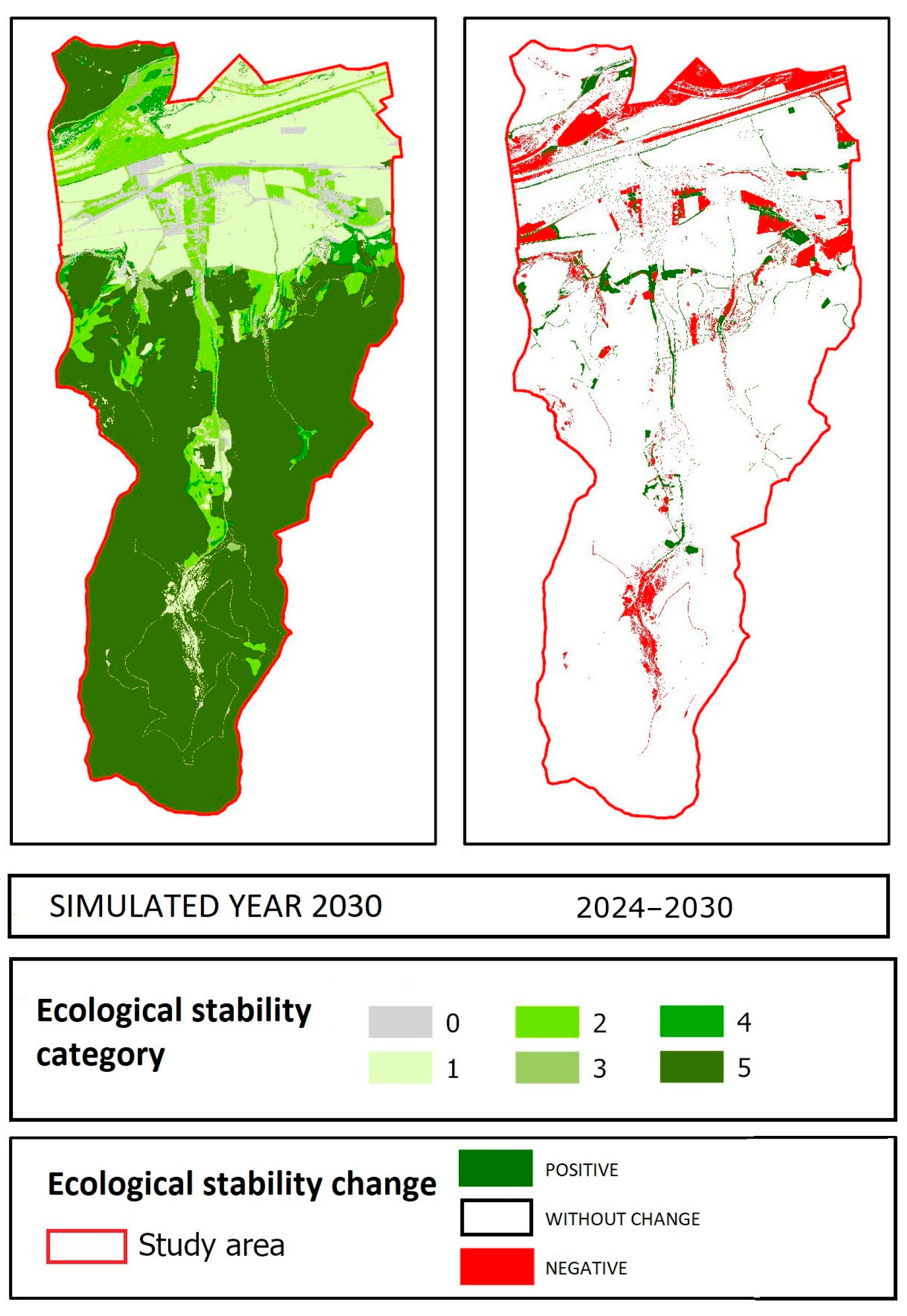
- Category 5 (very high significance) includes landscape elements with natural and near-natural vegetation (natural forests, natural grassland communities, wetlands, peatlands, watercourses, areas with natural beds and banks and with characteristic aquatic and riparian communities, etc.).
- Category 4 (high significance) includes landscape elements with semi-natural and near-natural vegetation (forests and meadows dominated by naturally occurring species, natural water bodies, etc.).
- Category 3 (moderate significance) includes landscape elements with anthropogenically influenced vegetation with natural elements (e.g., grassed and extensively used orchards, etc.).
- Category 2 (low significance) includes landscape elements with anthropogenically influenced synanthropic vegetation (e.g., intensively managed orchards, vineyards, reclaimed meadows, etc.).
- Category 1 (very low significance) includes elements such as intensively used, large-scale blocks of arable land, etc.
- Category 0 (no significance) includes elements like built-up areas, roads, etc.
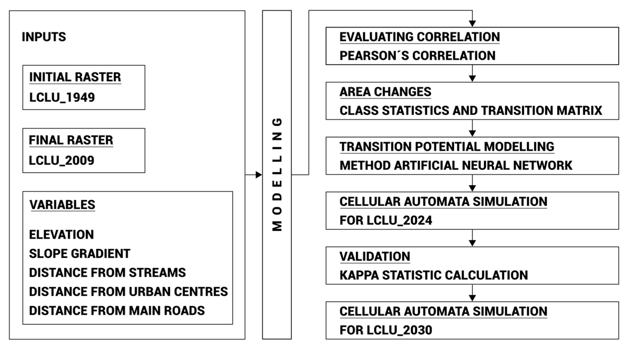
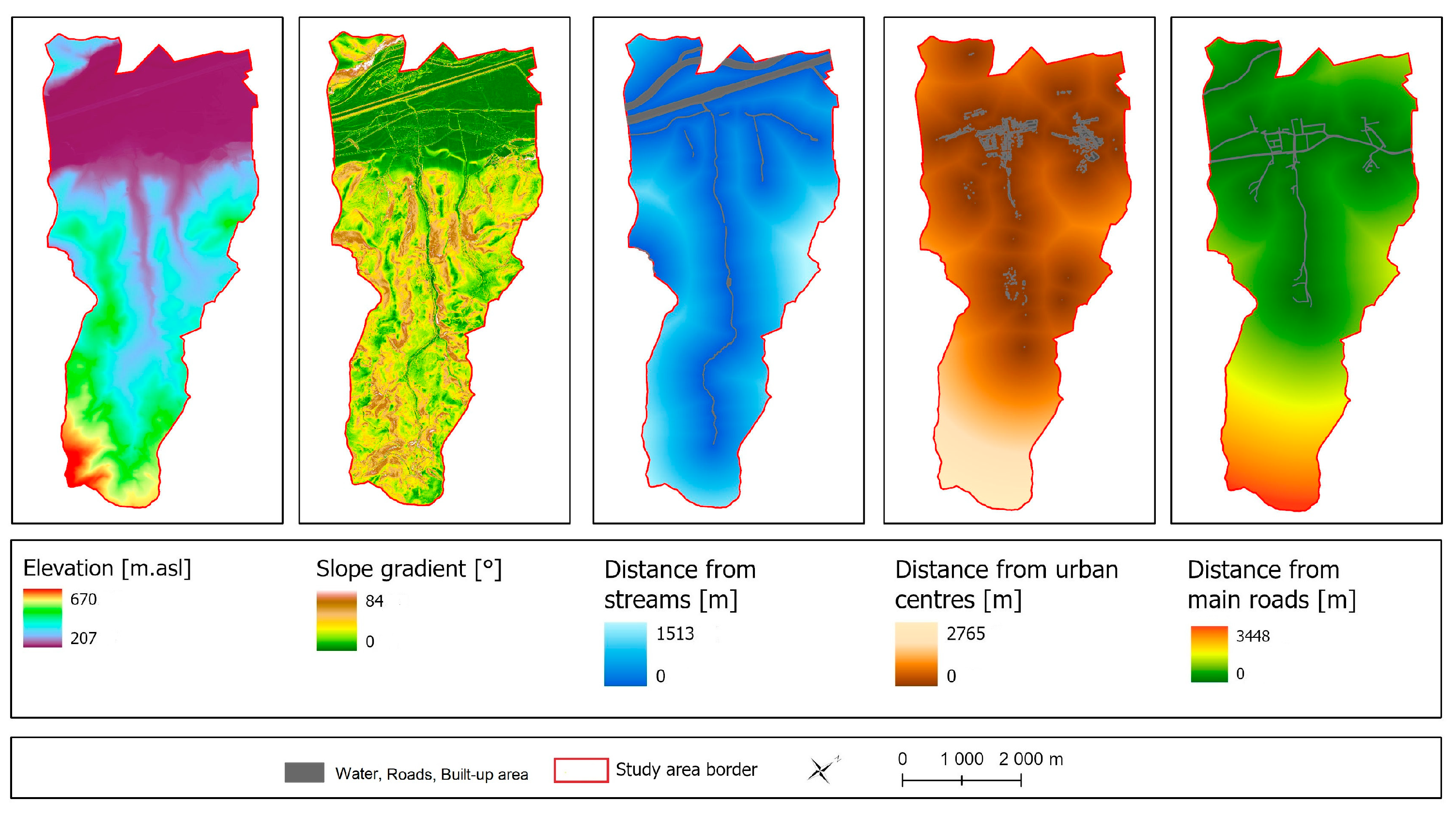
2.4. LULC Prediction
3. Results and Discussion
4. Conclusions
Author Contributions
Funding
Data Availability Statement
Conflicts of Interest
References
- Lambin, E.F.; Geist, H.J. Land-Use and Land-Cover Change: Local Processes and Global Impacts; Springer: Berlin/Heidelberg, Germany, 2006; p. 236. [Google Scholar]
- Jansen, L.J.M.; Di Gregorio, A. Parametric land cover and land-use classification as tools for environmental change detection. Agric. Ecosyst. Environ. 2002, 91, 89–100. [Google Scholar] [CrossRef]
- Patel, S.K.; Verma, P.; Singh, G.S. Agricultural growth and land use land cover change in peri-urban India. Environ. Monit. Assess. 2019, 191, 600. [Google Scholar] [CrossRef] [PubMed]
- Bununu, Y.A.; Bello, A.; Ahmed, A. Land cover, land use, climate change and food security. Sustain. Earth Rev. 2023, 6, 16. [Google Scholar] [CrossRef]
- Sherley, E.F.; Kumar, A.; Revathy, D. Detection and prediction of land use and land cover changes using deep learning. In Communication Software and Networks; Lecture Notes in Networks and Systems; Springer: Singapore, 2021; Volume 134, pp. 437–448. [Google Scholar] [CrossRef]
- Ives, A.R.; Carpenter, S.R. Stability and diversity of ecosystems. Science 2007, 317, 58–62. [Google Scholar] [CrossRef] [PubMed]
- Zaccarelli, N.; Petrosillo, I.; Zurlini, G. Retrospective analysis. In Encyclopedia of Ecology; Elsevier: Amsterdam, The Netherlands, 2008; pp. 3020–3029. [Google Scholar] [CrossRef]
- Cassin, J.; Matthews, J.H. Nature-based solutions, water security and climate change: Issues and opportunities. In Nature-Based Solutions and Water Security; Cassin, J., Matthews, J.H., Lopez Gunn, E., Eds.; Elsevier: Amsterdam, The Netherlands, 2021; pp. 63–79. [Google Scholar] [CrossRef]
- Donohue, I.; Hillebrand, H.; Montoya, J.M.; Petchey, O.L.; Pimm, S.L.; Fowler, M.S.; Healy, K.; Jackson, A.L.; Lurgi, M.; McClean, D.; et al. Navigating the complexity of ecological stability. Ecol. Lett. 2016, 19, 1172–1185. [Google Scholar] [CrossRef] [PubMed]
- Chromčák, J.; Bačová, D.; Pecho, P.; Seidlová, A. The possibilities of orthophotos application for calculation of ecological stability coefficient purposes. Sustainability 2021, 13, 3017. [Google Scholar] [CrossRef]
- Míchal, I. Principy krajinářského hodnocení území. Archit. A Urban 1982, 65, 87. [Google Scholar]
- Löw, J. Zásady Pro Vymezování a Navrhovaní Územních Systému Ekologické Stability; Agroprojekt: Brno, Czech Republic, 1984; p. 55. [Google Scholar]
- Miklós, L. Stabilita krajiny v ekologickom genereli SSR. Zivotn. Prostr. 1986, 20, 87–93. [Google Scholar]
- Gehrig-Fasel, J.; Guisan, A.; Zimmermann, N.E. Tree line shifts in the Swiss Alps: Climate change or land abandonment? J. Veg. Sci. 2007, 18, 571–582. [Google Scholar] [CrossRef]
- Halada, L.; Evans, D.; Romao, C.; Petersen, J.E. Which habitats of European importance depend on agricultural practices? Biodivers. Conserv. 2011, 20, 2365–2378. [Google Scholar] [CrossRef]
- Henle, K.; Alard, D.; Clitherow, J.; Cobb, P. Identifying and managing the conflicts between agriculture and biodiversity conservation in Europe—A review. Agric. Ecosyst. Environ. 2008, 124, 60–71. [Google Scholar] [CrossRef]
- Nguyen, H.Q.; Warr, P. Land consolidation as technical change: Economic impacts in rural Vietnam. World Dev. 2020, 127, 104750. [Google Scholar] [CrossRef]
- Janečková Molnárová, K.; Sklenička, P.; Bohnet, I.C.; Lowther-Harris, F.; Van den Brink, A.; Moghaddam, S.M.; Fanta, V.; Zástěra, V.; Azadi, H. Impacts of land consolidation on land degradation. J. Environ. Manag. 2023, 329, 117026. [Google Scholar] [CrossRef] [PubMed]
- Jiang, Y.; Long, H.; Tang, Y.; Deng, W.; Chen, K.; Zheng, Y. The impact of land consolidation on rural vitalization at village level: A case study of a Chinese village. J. Rural Stud. 2021, 86, 485–496. [Google Scholar] [CrossRef]
- Turner, B.L.; Lambin, E.F.; Reenberg, A. The emergence of land change science for global environmental change and sustainability. Proc. Natl. Acad. Sci. USA 2007, 104, 20666–20671. [Google Scholar] [CrossRef] [PubMed]
- Lu, D.; Moran, E.; Hetrick, S.; Li, G. Land-use and land-cover change detection. In Advances in Environmental Remote Sensing: Sensors, Algorithms and Applications; CRC Press: Boca Raton, FL, USA, 2011; pp. 273–291. [Google Scholar] [CrossRef]
- Seifu, T.K.; Woldesenbet, T.A.; Alemayehu, T.; Ayenew, T. Spatio-Temporal Change of Land Use/Land Cover and Vegetation Using Multi-MODIS Satellite Data, Western Ethiopia. Sci. World J. 2023, 2023, 7454137. [Google Scholar] [CrossRef] [PubMed]
- Muhammad, R.; Zhang, W.; Abbas, Z.; Guo, F.; Gwiazdzinski, L. Spatiotemporal Change Analysis and Prediction of Future Land Use and Land Cover Changes Using QGIS MOLUSCE Plugin and Remote Sensing Big Data: A Case Study of Linyi, China. Land 2022, 11, 419. [Google Scholar] [CrossRef]
- Zhang, Y.; Liu, X.; Chen, H.; Wang, L.; Li, J. Integrating Machine Learning and GIS for Predictive Mapping of Ecological Vulnerability Under Land Use Change Scenarios. Front. Environ. Sci. 2025, 13, 1540140. [Google Scholar] [CrossRef]
- Soil Science and Conservation Research Institute. Map Service. Available online: https://portal.vupop.sk/portal/apps/webappviewer/index.html?id=d89cff7c70424117ae01ddba7499d3ad (accessed on 5 October 2024).
- Muchová, Z.; Vanek, J.; Halaj, P.; Hrnčiarová, T.; Konc, Ľ.; Raškovič, V.; Streďanská, A.; Šimonides, I.; Vašek, A. Metodické Štandardy Projektovania Pozemkových Úprav, 1st ed.; SPU v Nitre: Nitra, Slovakia, 2009; p. 397. [Google Scholar]
- Löw, J. Rukověť Projektanta Místního Územního Systému Ekologické Stability; Doplňek: Brno, Czech Republic, 1995; p. 124. [Google Scholar]
- Verburg, P.H.; Alexander, P.; Evans, T.; Magliocca, N.R.; Malek, Z.; Rounsevell, M.D.A. Beyond land cover change: Towards a new generation of land use models. Curr. Opin. Environ. Sustain. 2019, 38, 77–85. [Google Scholar] [CrossRef]
- Li, Z.; Jiang, W.; Peng, K.; Wang, X.; Deng, Y.; Yin, X.; Ling, Z. Comparative analysis of land use change prediction models for land and fine wetland types: Taking the wetland cities Changshu and Haikou as examples. Landsc. Urban Plan. 2024, 243, 104975. [Google Scholar] [CrossRef]
- Ward, D.P.; Murray, A.T.; Phinn, S.R. A stochastically constrained cellular model of urban growth. Comput. Environ. Urban Syst. 2000, 24, 539–558. [Google Scholar] [CrossRef]
- Alam, N.; Saha, S.; Gupta, S.; Chakraborty, S. Prediction modelling of riverine landscape dynamics in the context of sustainable management of floodplain: Geospatial approach. Ann. GIS 2021, 27, 299–314. [Google Scholar] [CrossRef]
- Rahman, M.T.U.; Tabassum, F.; Rasheduzzaman, M.; Saba, H.; Sarkar, L.; Ferdous, J.; Uddin, S.Z.; Zahedul Islam, A.Z.M. Temporal dynamics of land use/land cover change and its prediction using CA-ANN model for southwestern coastal Bangladesh. Environ. Monit. Assess. 2017, 189, 565. [Google Scholar] [CrossRef] [PubMed]
- Hamad, R.; Balzter, H.; Kolo, K. Predicting land use/land cover changes using a CA-Markov model under two different scenarios. Sustainability 2018, 10, 3421. [Google Scholar] [CrossRef]
- Praveen, R.; Kanmani, S. Predicting the future land use and land cover changes for Bhavani basin, Tamil Nadu, India, using QGIS MOLUSCE plugin. Environ. Sci. Pollut. Res. 2021, 28, 58724–58736. [Google Scholar] [CrossRef]
- Foody, G.M. Explaining the unsuitability of the kappa coefficient in the assessment and comparison of the accuracy of thematic maps obtained by image classification. Remote Sens. Environ. 2020, 239, 111630. [Google Scholar] [CrossRef]
- Kuemmerle, T.; Hostert, P.; Radeloff, V.C.; van der Linden, S.; Perzanowski, K.; Kruhlov, I. Cross-Border Comparison of Post-Socialist Farmland Abandonment in the Carpathians. Ecosystems 2008, 11, 614–628. [Google Scholar] [CrossRef]
- Munteanu, C.; Kuemmerle, T.; Boltiziar, M.; Butsic, V.; Gimmi, U.; Halada, L.; Radeloff, V.C. Forest and Agricultural Land Change in the Carpathian Region—A Meta-Analysis of Long-Term Patterns and Drivers. Land Use Policy 2014, 38, 685–697. [Google Scholar] [CrossRef]
- Petrovič, F.; Muchová, Z.; Lieskovský, J. Assessment of Ecological Stability Development of Agricultural Landscape on the Basis of Land Use Changes (Case Study: Nitra Region). Ekologia 2016, 35, 38–49. [Google Scholar] [CrossRef]
- Esch, T.; Marconcini, M.; Felbier, A.; Roth, A.; Heldens, W.; Huber, M.; Dech, S. Urban Footprint Processor—Fully Automated Processing Chain Generating Settlement Masks from Global Data of the Copernicus Programme. Remote Sens. Environ. 2020, 242, 111744. [Google Scholar] [CrossRef]
- Šišmiš, M.Z. Dejín Opatovej Nad Váhom do Roku 1918. Opatova.sk. Available online: https://www.vkmr.sk/buxus/docs/Pravek%C3%A9%20a%20v%C4%8Dasnohistorick%C3%A9%20archeologick%C3%A9%20n%C3%A1lezisk%C3%A1%20v%20tren%C4%8Dianskom%20regi%C3%B3ne.pdf (accessed on 11 April 2017).
- Alshari, E.A.; Gawali, B.W. Modeling land use change in Sana’a City of Yemen with MOLUSCE. J. Sens. 2022, 15, 7419031. [Google Scholar] [CrossRef]
- Friehat, T.; Mulugeta, G.; Gala, T. Modeling urban sprawls in northeastern Illinois. J. Geosci. 2015, 3, 133–141. [Google Scholar] [CrossRef]
- Mondal, D.M.S.; Sharma, N.; Kappas, M.; Garg, P. CA MARKOV modeling of land use land cover change predictions and effect of numerical iterations, image interval (time steps) on prediction results. Int. Arch. Photogramm. Remote Sens. Spatial Inf. Sci. 2020, 43, 713–720. [Google Scholar] [CrossRef]
- Rahmi, K.; Ali, A.; Maghribi, A.; Aldiansyah, S.; Atiqi, R. Monitoring of land use land cover change using Google Earth Engine in urban area: Kendari city 2000–2021. IOP Conf. Ser. Earth Environ. Sci. 2022, 950, 012081. [Google Scholar] [CrossRef]


| Land-Use Element Subdivisions (Unique Code) | Occurrence of the Element in the Given Year Marked with x | Land-Use Element Subdivisions (Unique Code) | Occurrence of the Element in the Given Year Marked with x | ||||||
|---|---|---|---|---|---|---|---|---|---|
| 1850 | 1949 | 2009 | 2024 | 1850 | 1949 | 2009 | 2024 | ||
| Large-block arable land (0210001) | x | x | Grass-covered yard with planted settlement vegetation (1310403) | x | x | x | |||
| Small-block arable land–strip fields (0210002) | x | x | x | x | Non-residential development (1320001, 1320002) | x | x | x | |
| Garden outside the built-up area (0510001) | x | x | Railway tracks (1330101) | x | x | x | |||
| Orchard (0610001) | x | x | x | Aerial ropeways (1330103) | x | x | |||
| Abandoned orchard (0610003) | x | x | First-class road (1332101) | x | x | x | x | ||
| Abandoned meadows and pastures (weedy) (0710014) | x | x | x | Local road (1332102) | x | x | x | x | |
| Intensively used meadows (0710001) | x | x | Sidewalk (1332103) | x | x | ||||
| Semi-intensively used meadows (0710002) | x | x | x | x | Other road objects (e.g., guardrails, signs) (1332104) | x | x | ||
| Extensively used meadows (0710004) | x | x | Paved field road (1332105) | x | x | ||||
| Semi-intensively used pastures (0710009) | x | x | Wastewater treatment plant (1336104) | x | x | ||||
| Abandoned meadows and pastures with shrubs (NDV) (0710018) | x | x | x | Water reservoir (1336106) | x | x | |||
| Temporarily removed forest cover–clear-cut area (1020039) | x | Weir (1336108) | x | ||||||
| Forest storage (1023002) | x | x | Construction site (1370001) | x | x | ||||
| Unpaved forest road (1023003) | x | x | Mill (1427000) | x | |||||
| Beech and fir–beech forests (1020012) | x | x | x | x | Industrial area (1427002) | x | |||
| Paved forest road (1026002) | x | x | Abandoned quarry (1428002) | x | |||||
| Watercourse with natural channel (1111001) | x | x | Street vegetation (1441003) | x | |||||
| Watercourse with modified channel (1111002) | x | x | NDV—forest ecosystem fragments (1442006) | x | x | x | x | ||
| Seasonal watercourse (1111004) | x | Playground (1450003) | x | x | |||||
| Canal (1111005) | x | x | Cottage settlement area (1450005) | x | x | ||||
| Canal with overgrown channel (1111006) | x | x | x | Cemetery (1460001) | x | x | x | x | |
| Water body (1111007) | x | x | Gully or ravine (1470007) | x | x | ||||
| Riparian grass and herb vegetation (1113008) | x | x | Natural rock formations (1470008) | x | x | ||||
| Spring area (1113010) | x | x | Gravel banks (1470009) | x | x | ||||
| Wetlands with fluctuating water levels (1113014) | x | x | Unpaved field road (1473001) | x | x | x | |||
| Family housing (1310002) | x | x | x | x | Unpaved field manure pit (1473004) | x | |||
| Isolated residential structures (1310003) | x | x | Sacred building (church, monastery) (1480006) | x | x | x | x | ||
| Concrete-paved yard (1310401) | x | x | x | Wayside shrine (1480008) | x | x | |||
| Grass-covered yard (1310402) | x | x | |||||||
| Land Type | 1850 | 1949 | 2009 | 2024 | ||||
|---|---|---|---|---|---|---|---|---|
| ha | % | ha | % | ha | % | ha | % | |
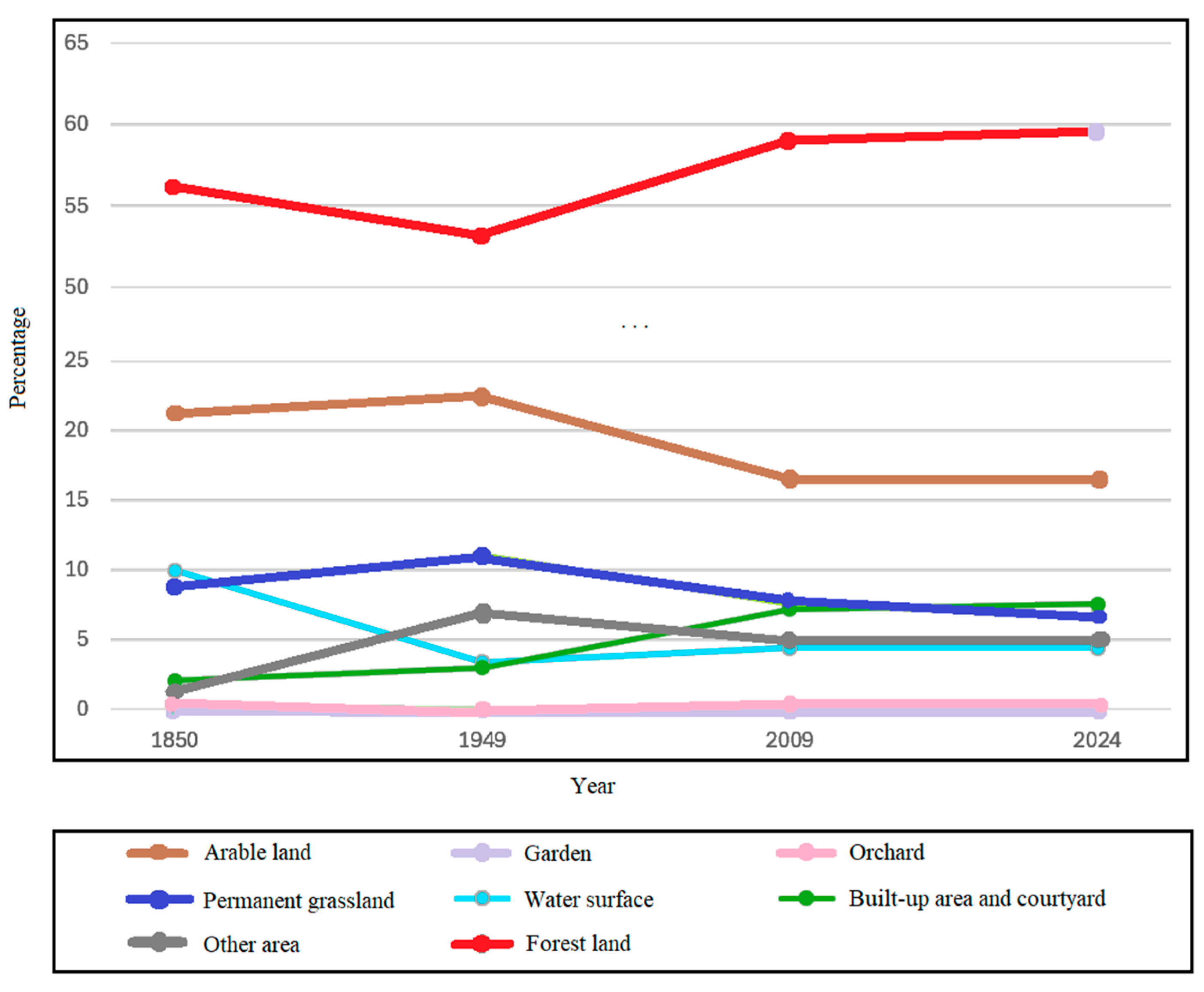
| Arable land | 416.03 | 21.29 | 438.22 | 22.43 | 324.54 | 16.61 | 321.59 | 16.46 |
| Garden | 0.00 | 0.00 | 0.00 | 0.00 | 1.80 | 0.09 | 0.51 | 0.03 |
| Orchard | 6.14 | 0.31 | 0.00 | 0.00 | 3.65 | 0.19 | 3.88 | 0.20 |
| Permanent grassland | 172.17 | 8.81 | 215.37 | 11.02 | 147.77 | 7.56 | 131.59 | 6.73 |
| Forest land | 1097.19 | 56.15 | 1040.00 | 53.22 | 1152.86 | 59.00 | 1164.64 | 59.60 |
| Water surface | 195.50 | 10.00 | 66.58 | 3.41 | 86.55 | 4.43 | 86.69 | 4.44 |
| Built-up area and courtyard | 40.33 | 2.06 | 59.10 | 3.02 | 140.81 | 7.21 | 147.82 | 7.57 |
| Other area | 26.68 | 1.37 | 134.73 | 6.90 | 96.06 | 4.92 | 97.28 | 4.98 |
| Category | 1850–1949 | 1949–2009 | 2009–2024 |
|---|---|---|---|
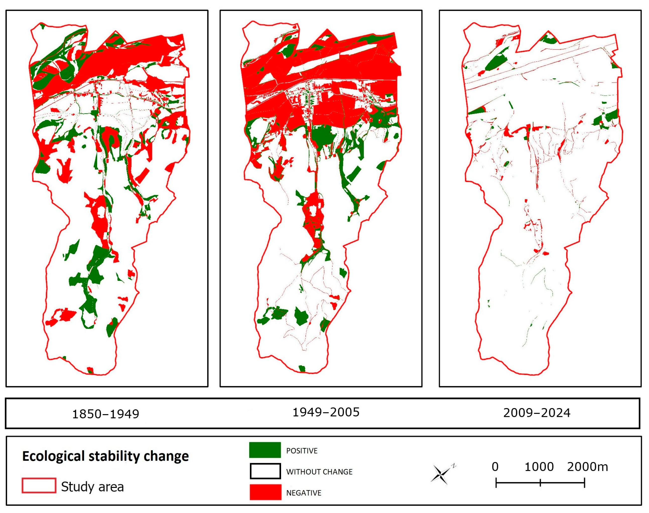
| Positive | 11.41 | 10.32 | 2.13 |
| Negative | 19.93 | 28.40 | 2.49 |
| Without change | 68.66 | 61.29 | 95.38 |
Disclaimer/Publisher’s Note: The statements, opinions and data contained in all publications are solely those of the individual author(s) and contributor(s) and not of MDPI and/or the editor(s). MDPI and/or the editor(s) disclaim responsibility for any injury to people or property resulting from any ideas, methods, instructions or products referred to in the content. |
© 2025 by the authors. Licensee MDPI, Basel, Switzerland. This article is an open access article distributed under the terms and conditions of the Creative Commons Attribution (CC BY) license (https://creativecommons.org/licenses/by/4.0/).
Share and Cite
Tárníková, M.; Muchová, Z. Ecological Stability over the Period: Land-Use Land-Cover Change and Prediction for 2030. Land 2025, 14, 1503. https://doi.org/10.3390/land14071503
Tárníková M, Muchová Z. Ecological Stability over the Period: Land-Use Land-Cover Change and Prediction for 2030. Land. 2025; 14(7):1503. https://doi.org/10.3390/land14071503
Chicago/Turabian StyleTárníková, Mária, and Zlatica Muchová. 2025. "Ecological Stability over the Period: Land-Use Land-Cover Change and Prediction for 2030" Land 14, no. 7: 1503. https://doi.org/10.3390/land14071503
APA StyleTárníková, M., & Muchová, Z. (2025). Ecological Stability over the Period: Land-Use Land-Cover Change and Prediction for 2030. Land, 14(7), 1503. https://doi.org/10.3390/land14071503