


Best Siting for Small Hill Reservoirs and the Challenge of Sedimentation: A Case Study in the Umbria Region (Central Italy)


Abstract
1. Introduction
2. Materials and Methods
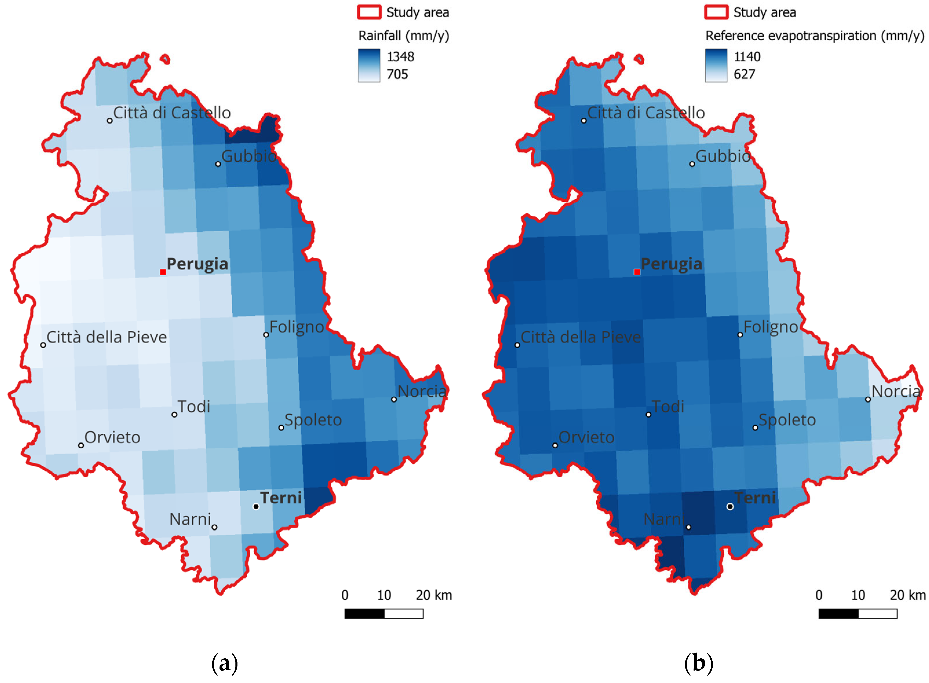
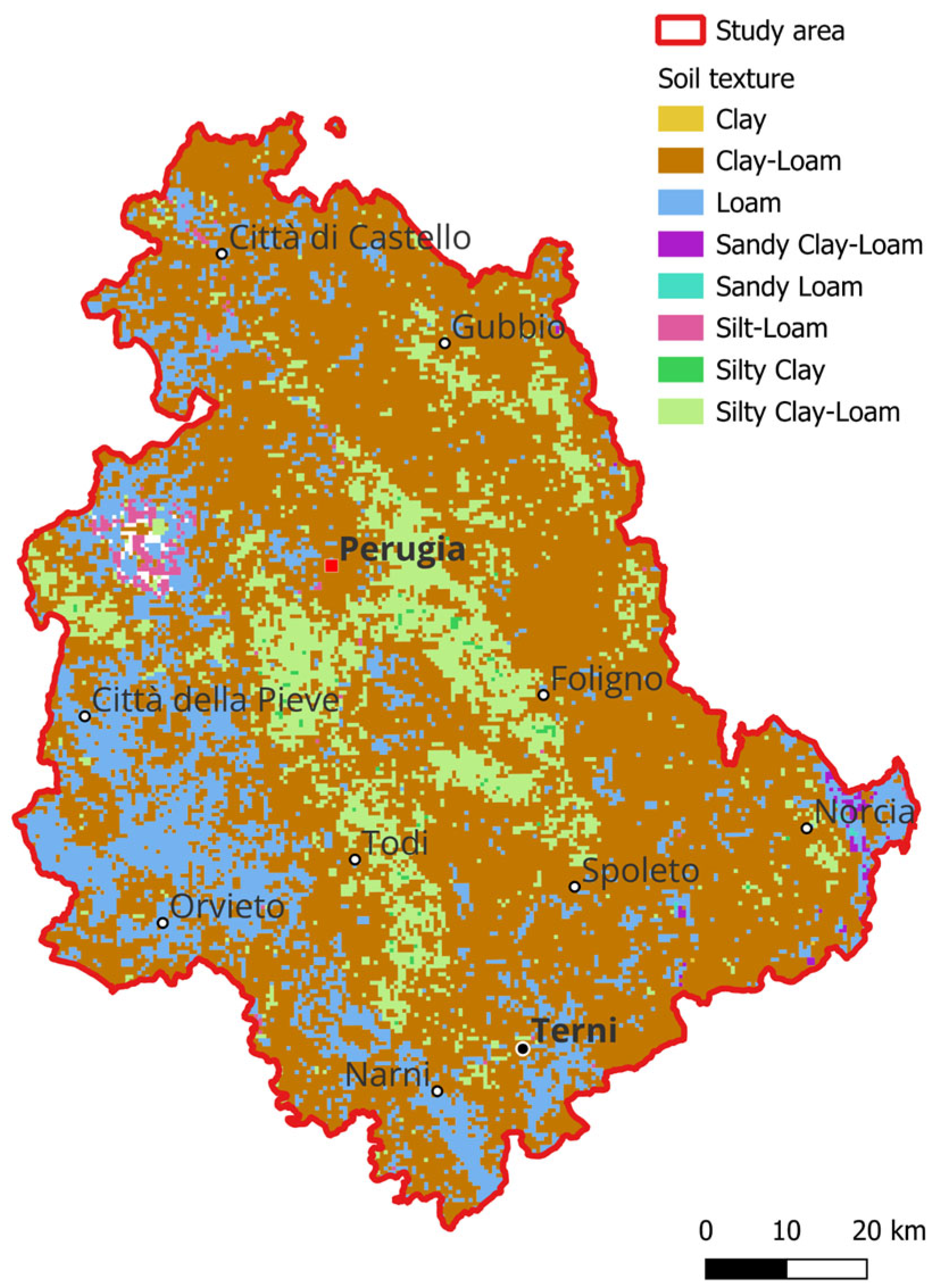
2.1. Study Area
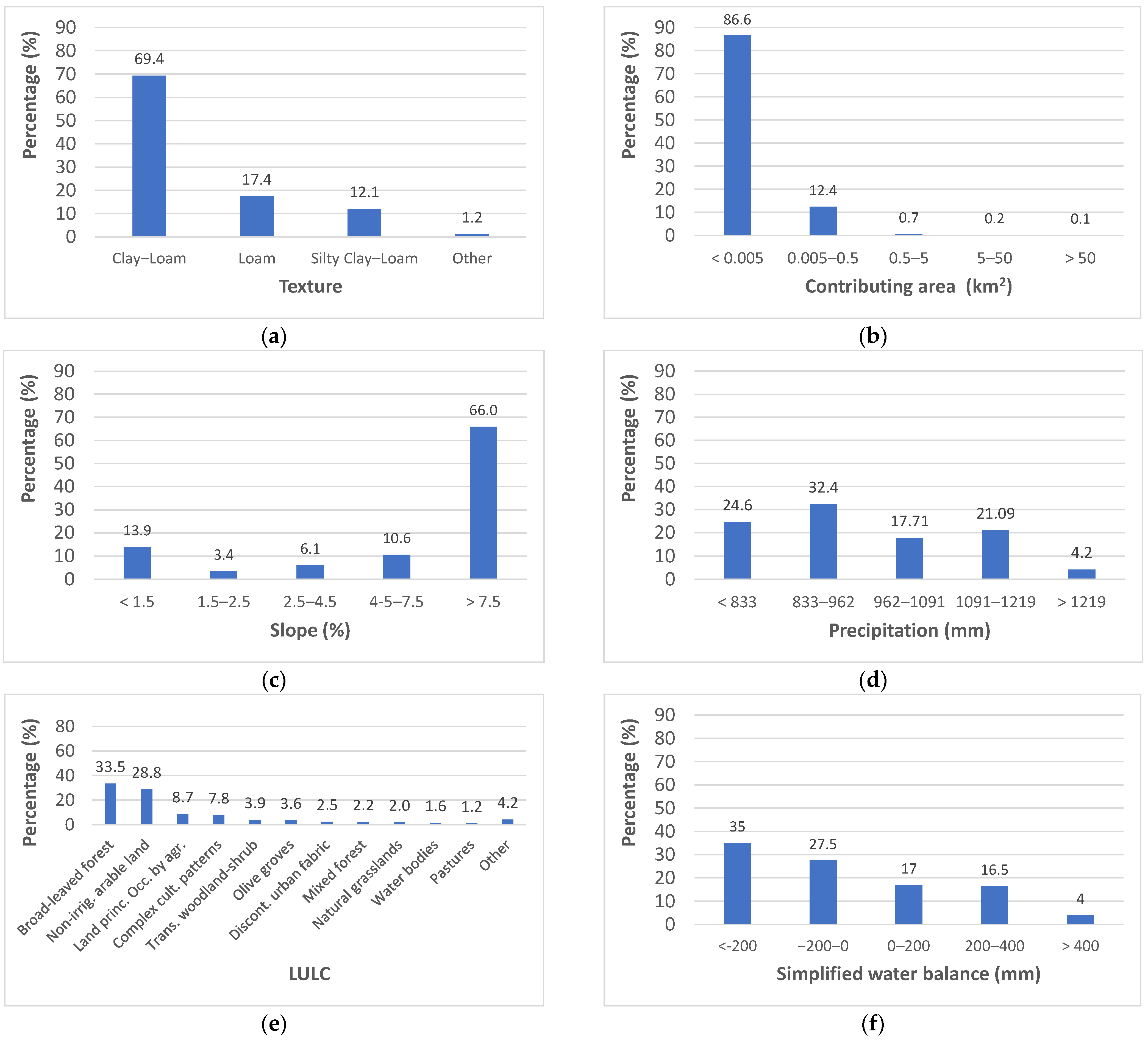
2.2. Data
2.2.1. Topographic, Meteorological, Soil and Land Use Data
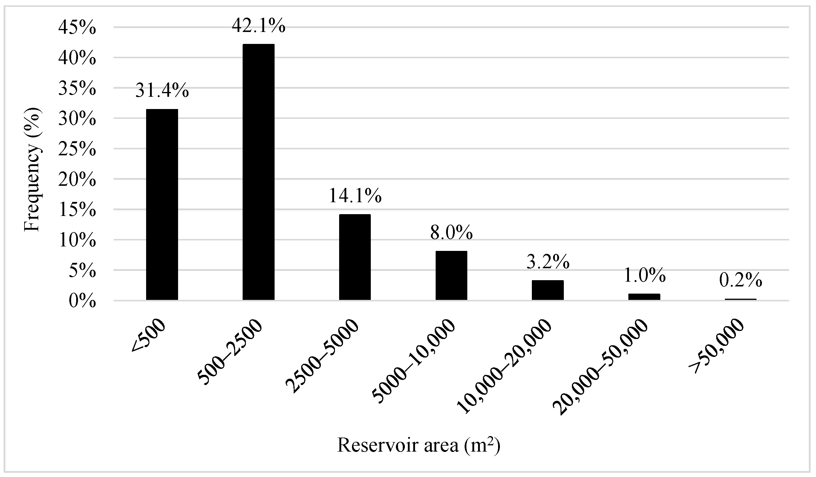
2.2.2. Database of Existing Reservoirs
2.3. Methods
2.3.1. Weighted Overlay Process
- Defining the criteria, i, considered relevant for determining suitability;
- Defining the classes, c, within each criterion;
- Establishing a scale of normalized suitability scores si,c for each class (e.g., from 1 to 5 or from 1 to 10) within each criterion;
- Optionally assigning different weights, wi, to each criterion based on their relative importance;
- Computing the suitability score (Ssu) for each cell to produce the final suitability map as follows:
2.3.2. Model A
2.3.3. Model B
- 1.
- Assignment of a unique class per criterion to each reservoir
- 2.
- Computation of the weighted frequency () for each class c
- 3.
- Ranking and scoring
2.3.4. Suitability Evaluation Based on Sediment Yield (Model C)
2.3.5. Evaluation of Agreement Between Suitability Models
3. Results
3.1. Definition of the Suitability Scores for Model B
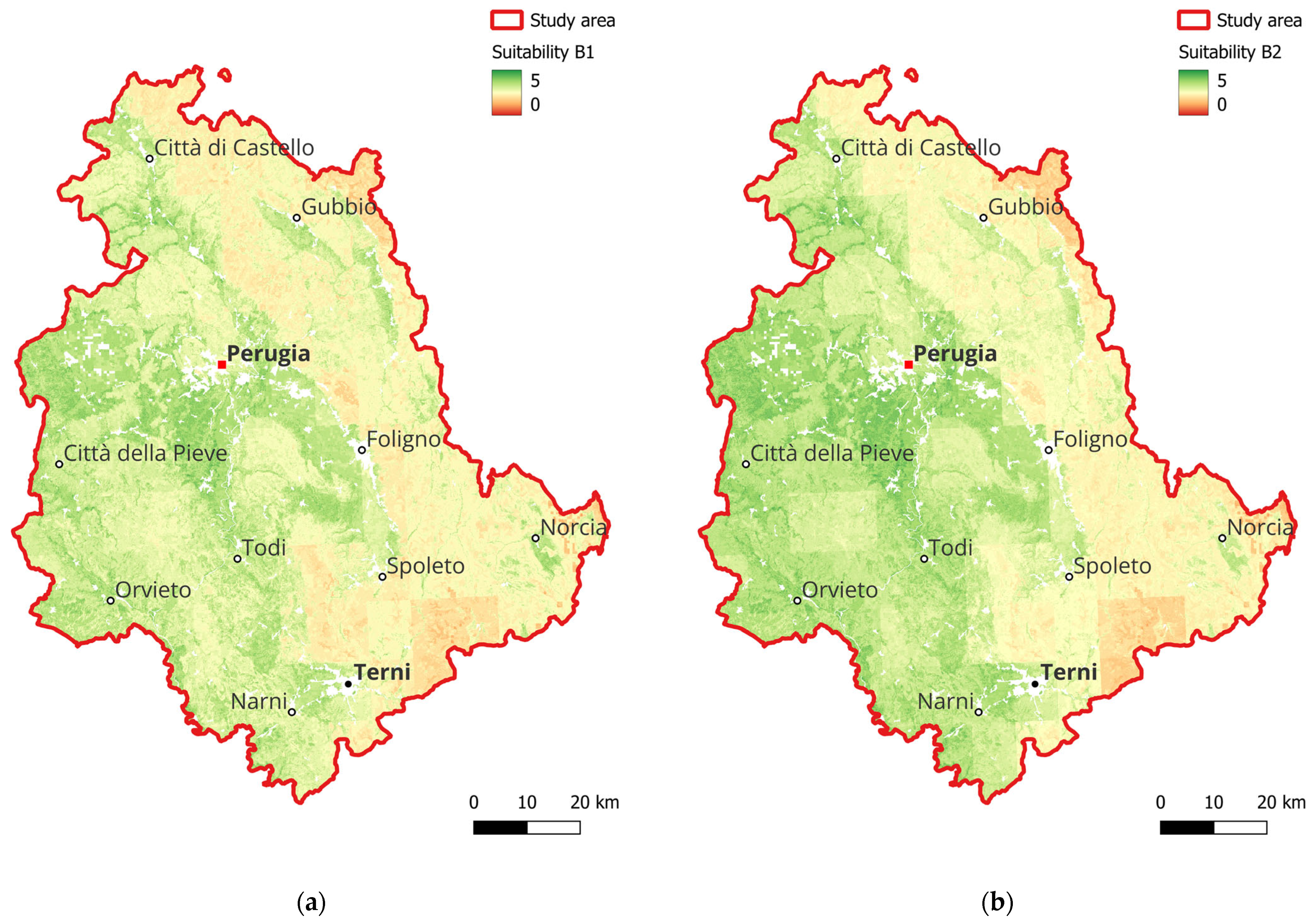
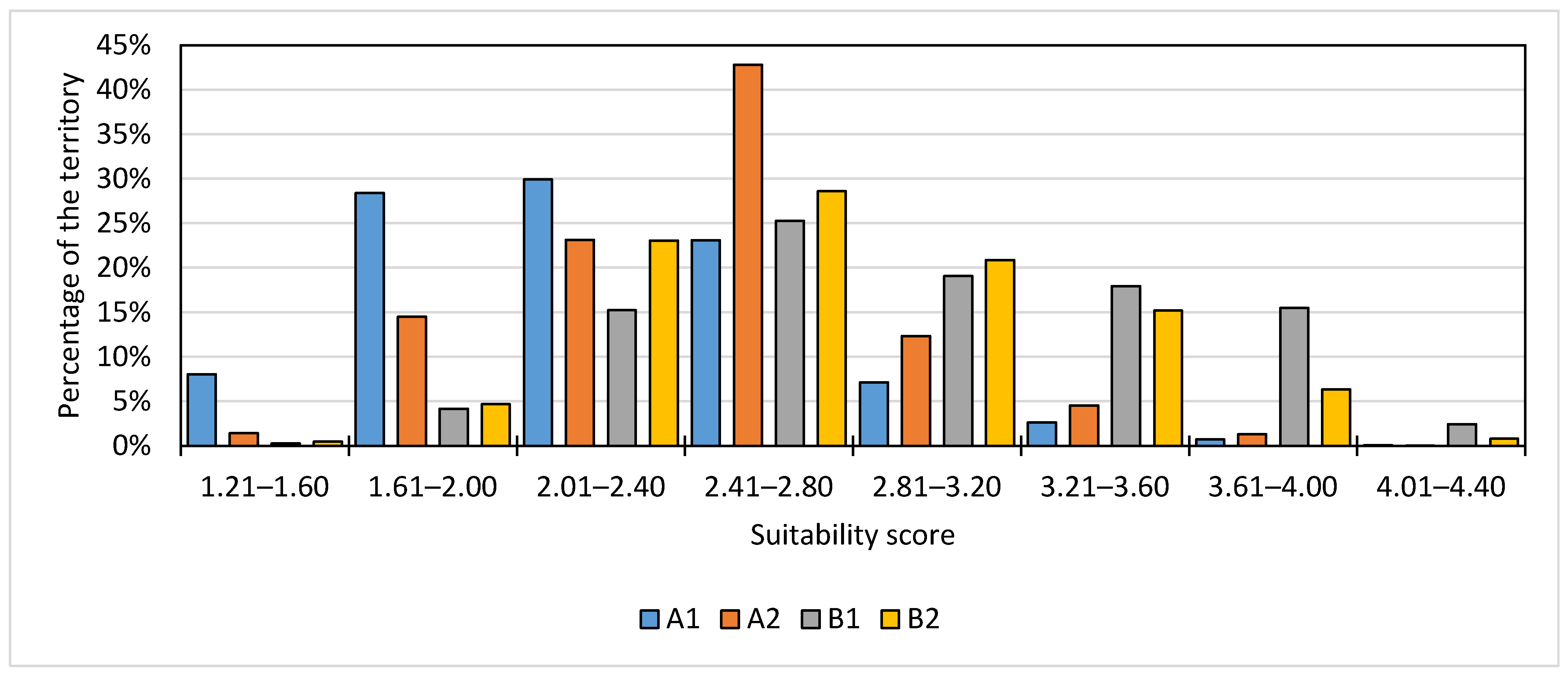
3.2. Suitability Maps Based on Model A and Model B
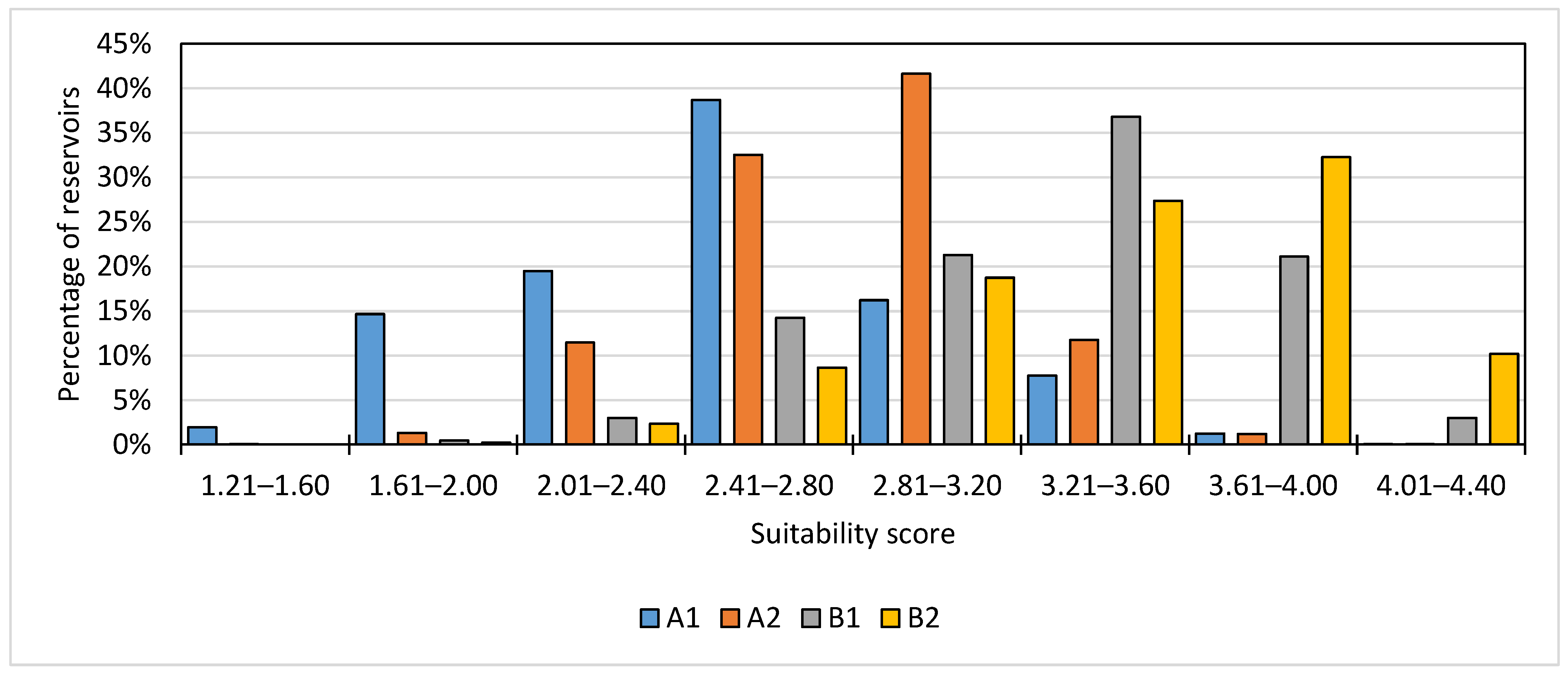
3.3. Potential Sediment Production and Siltation Risk on Existing Reservoirs
4. Discussion
5. Conclusions
Author Contributions
Funding
Data Availability Statement
Acknowledgments
Conflicts of Interest
Abbreviations
| CA | Contributing Area |
| ET0 | Annual reference evapotranspiration |
| MCDM | Multi-Criteria Decision-Making |
| LULC | Land Use Land Cover |
| Pr | Annual precipitation |
| RUSLE | Revised Universal Soil Loss Equation |
| SHRBS | Small Hill Reservoir Best Siting |
| SHR Sl | Small Hill Reservoir Slope |
| T | Texture |
| WB | Simplified water balance |
| WOP | Weighted Overlay Process |
Appendix A

| Criterion | Suitability Score | ||||
|---|---|---|---|---|---|
| 5 (Highly Suitable) | 4 | 3 | 2 | 1 (Low Suitability) | |
| Texture, T | Clay | Silty-clay | Sandy-clay | Sandy-clay-loam, Sandy-loam | Clay-loam, Silt, Silt-loam, Loam, Sand, Loamy-sand, Silty-clay-loam |
| Contributing Area, CA (km2) | 0.005–0.5 | 0.5–5 | 5–50 | <0.005 | >50 |
| Slope, Sl (%) | 1.5–2.5 | 2.5–4.5 | <1.5 | 4.5–7.5 | >7.5 |
| Precipitation, Pr (mm/year) | 962–1091 | 1091–1219 | 833–962 | >1219 | <833 |
| LULC | Sparsely vegetated areas, inland marshes, pastures, natural grasslands, non-irrigated arable land, predominantly agricultural land with significant natural vegetation areas, water bodies | Fruit trees and berry plantations, annual crops associated with permanent crops, complex cultivation patterns, olive groves, sclerophyllous vegetation, vineyards | Burnt areas, transitional shrubland-forest | Broad-leaved forest, mixed forest, coniferous forest | Bare rocks, mining sites, beaches, dunes, sands |
| Simplified Water Balance, WB (mm/year) | <−200 | −200–0 | 0–200 | 200–400 | >400 |
| Criterion | Suitability Score | ||||
|---|---|---|---|---|---|
| 5 (Highly Suitable) | 4 | 3 | 2 | 1 (Low Suitability) | |
| Texture, T | Silty Clay-Loam, Loam | Clay-Loam | Silty-Clay, Silt-Loam | - | Clay, Sandy-Clay-Loam, Sandy-Loam |
| Contributing Area, CA (km2) | 0.5–5 | 5–50 | >50 | 0.005–0.5 | <0.005 |
| Slope, Sl (%) | 1.5–2.5 | 2.5–4.5 | 4.5–7.5 | <1.5 | >7.5 |
| Precipitation, Pr (mm/year) | <883 | 833–962 | 962–1091 | 1091–1219 | >1219 |
| LULC | Inland marshes, Mineral extraction sites, Fruit trees and berry plantations, Water bodies, Non-irrigated arable land | Water courses, Land principally occupied by agriculture with significant areas of natural vegetation, Complex cultivation patterns, Vineyards | Mixed forest, Sclerophyllous vegetation, Pastures, Olive groves, Broad-leaved forest | Natural grasslands, Transitional woodland-shrub | Annual crops associated with permanent crops, Bare rocks, Beaches, dunes, sands, Burnt areas, Coniferous forest, Construction sites, Sparsely vegetated areas |
| Simplified Water Balance, WB (mm/year) | <−200 | −200–0 | 200–400 | 0–200 | >400 |
References
- Adhikari, S. Drought Impact and Adaptation Strategies in the Mid-Hill Farming System of Western Nepal. Environments 2018, 5, 101. [Google Scholar] [CrossRef]
- Ferk, M.; Ciglič, R.; Komac, B.; Loczy, D. Management of Small Retention Ponds and Their Impact on Flood Hazard Prevention in the Slovenske Gorice Hills. AGS 2020, 60, 107–125. [Google Scholar] [CrossRef]
- Adham, A.; Sayl, K.N.; Abed, R.; Abdeladhim, M.A.; Wesseling, J.G.; Riksen, M.; Fleskens, L.; Karim, U.; Ritsema, C.J. A GIS-Based Approach for Identifying Potential Sites for Harvesting Rainwater in the Western Desert of Iraq. Int. Soil Water Conserv. Res. 2018, 6, 297–304. [Google Scholar] [CrossRef]
- Subedi, A.; Kalauni, D.; Khadka, R.; Kattel, R.R. Assessment of Role of Water Harvesting Technology in Vegetable-Based Income Diversification in Palpa District, Nepal. Cogent Food Agric. 2020, 6, 1758374. [Google Scholar] [CrossRef]
- Forzini, E.; Piemontese, L.; Bresci, E.; Barthod, B.; Bielser, F.; Sylvestre, M.; Adhikari, N.; Pun, S.; Castelli, G. Identification of Suitable Sites for Traditional Pokhari Water Harvesting in Mountain Rural Communities of the Himalaya. Hydrol. Res. 2022, 53, 1340–1356. [Google Scholar] [CrossRef]
- Di Francesco, S.; Casadei, S.; Di Mella, I.; Giannone, F. The Role of Small Reservoirs in a Water Scarcity Scenario: A Computational Approach. Water Resour Manag. 2022, 36, 875–889. [Google Scholar] [CrossRef]
- Casadei, S.; Di Francesco, S.; Giannone, F.; Pierleoni, A. Small Reservoirs for a Sustainable Water Resources Management. Adv. Geosci. 2019, 49, 165–174. [Google Scholar] [CrossRef]
- U.S. Department of Agriculture (USDA). Ponds-Planning, Design, Construction; Handbook AH-59; USDA: Washington, DC, USA, 1997; 85p.
- Adham, A.; Riksen, M.; Ouessar, M.; Ritsema, C. A Methodology to Assess and Evaluate Rainwater Harvesting Techniques in (Semi-) Arid Regions. Water 2016, 8, 198. [Google Scholar] [CrossRef]
- Dile, Y.T.; Rockström, J.; Karlberg, L. Suitability of Water Harvesting in the Upper Blue Nile Basin, Ethiopia: A First Step towards a Mesoscale Hydrological Modeling Framework. Adv. Meteorol. 2016, 2016, 5935430. [Google Scholar] [CrossRef]
- Mugo, G.M.; Odera, P.A. Site Selection for Rainwater Harvesting Structures in Kiambu County-Kenya. Egypt. J. Remote Sens. Space Sci. 2019, 22, 155–164. [Google Scholar] [CrossRef]
- Shadmehri Toosi, A.; Ghasemi Tousi, E.; Ghassemi, S.A.; Cheshomi, A.; Alaghmand, S. A Multi-Criteria Decision Analysis Approach towards Efficient Rainwater Harvesting. J. Hydrol. 2020, 582, 124501. [Google Scholar] [CrossRef]
- Umukiza, E.; Abagale, F.K.; Apusiga Adongo, T.; Petroselli, A. Suitability Assessment and Optimization of Small Dams and Reservoirs in Northern Ghana. Hydrology 2024, 11, 166. [Google Scholar] [CrossRef]
- Arabatzis, G.; Kolkos, G.; Stergiadou, A.; Kantartzis, A.; Tampekis, S. Optimal Allocation of Water Reservoirs for Sustainable Wildfire Prevention Planning via AHP-TOPSIS and Forest Road Network Analysis. Sustainability 2024, 16, 936. [Google Scholar] [CrossRef]
- Hosseinzadeh, A.; Behzadian, K.; Rossi, P.; Karami, M.; Ardeshir, A.; Torabi Haghighi, A. A New Multi-criteria Framework to Identify Optimal Detention Ponds in Urban Drainage Systems. J. Flood Risk Manag. 2023, 16, e12890. [Google Scholar] [CrossRef]
- Ouechtati, S.; Baldassarre, G. Evaluation Du Transport Solide et de l’envasement Dans Le Bassin Versant de Siliana (Tunisie): Cas Des Barrages Siliana et Lakhmess. Bull. Eng. Geol. Environ. 2011, 70, 709–722. [Google Scholar] [CrossRef]
- Todisco, F.; Tosi, G.; Vergni, L.; Marconi, L.; Radicioni, F. Sediment Volume Determination and Actualization of the Area-Volume-Elevation Curve in a Small Reservoir. In Biosystems Engineering Promoting Resilience to Climate Change—AIIA 2024—Mid-Term Conference; Sartori, L., Tarolli, P., Guerrini, L., Zuecco, G., Pezzuolo, A., Eds.; Lecture Notes in Civil Engineering; Springer Nature Switzerland: Cham, Switzerland, 2025; Volume 586, pp. 256–264. ISBN 978-3-031-84211-5. [Google Scholar]
- Banasik, K.; Hejduk, L.; Krajewski, A.; Wasilewicz, M. The Intensity of Siltation of a Small Reservoir in Poland and Its Relationship to Environmental Changes. CATENA 2021, 204, 105436. [Google Scholar] [CrossRef]
- Honek, D.; Michalková, M.Š.; Smetanová, A.; Sočuvka, V.; Velísková, Y.; Karásek, P.; Konečná, J.; Németová, Z.; Danáčová, M. Estimating Sedimentation Rates in Small Reservoirs—Suitable Approaches for Local Municipalities in Central Europe. J. Environ. Manag. 2020, 261, 109958. [Google Scholar] [CrossRef]
- Stanford University; University of Minnesota; Chinese Academy of Sciences; The Nature Conservancy; World Wildlife Fund; Stockholm Resilience Centre and the Royal Swedish Academy of Sciences. Natural Capital Project; InVEST, 3.16.0; Stanford University: Stanford, CA, USA; University of Minnesota: Minneapolis, MN, USA; Chinese Academy of Sciences: Beijing, China; The Nature Conservancy: Arlington, VA, USA; World Wildlife Fund: Gland, Switzerland; Stockholm Resilience Centre and the Royal Swedish Academy of Sciences: Stockholm, Sweden, 2025. [Google Scholar]
- Cornes, R.C.; Van Der Schrier, G.; Van Den Besselaar, E.J.M.; Jones, P.D. An Ensemble Version of the E-OBS Temperature and Precipitation Data Sets. JGR Atmos. 2018, 123, 9391–9409. [Google Scholar] [CrossRef]
- Hargreaves, G.H.; Zohrab, A. Samani Reference Crop Evapotranspiration from Temperature. Appl. Eng. Agric. 1985, 1, 96–99. [Google Scholar] [CrossRef]
- Tarquini, S.; Isola, I.; Favalli, M.; Battistini, A.; Dotta, G. TINITALY, a Digital Elevation Model of Italy with a 10 Meters Cell Size, Version 1.1; Istituto Nazionale di Geofisica e Vulcanologia (INGV): Rome, Italy, 2023. [Google Scholar]
- Ballabio, C.; Panagos, P.; Monatanarella, L. Mapping Topsoil Physical Properties at European Scale Using the LUCAS Database. Geoderma 2016, 261, 110–123. [Google Scholar] [CrossRef]
- European Environment Agency. CORINE Land Cover 2018 (Raster 100 m), Europe, 6-Yearly; Version 2020_20u1 May 2020; European Environment Agency: Copenhagen, Denmark, 2019. [Google Scholar]
- Taherdoost, H.; Madanchian, M. Multi-Criteria Decision Making (MCDM) Methods and Concepts. Encyclopedia 2023, 3, 77–87. [Google Scholar] [CrossRef]
- Adham, A.; Riksen, M.; Abed, R.; Shadeed, S.; Ritsema, C. Assessing Suitable Techniques for Rainwater Harvesting Using Analytical Hierarchy Process (AHP) Methods and GIS Techniques. Water 2022, 14, 2110. [Google Scholar] [CrossRef]
- Owusu, S.; Mul, M.L.; Ghansah, B.; Osei-Owusu, P.K.; Awotwe-Pratt, V.; Kadyampakeni, D. Assessing Land Suitability for Aquifer Storage and Recharge in Northern Ghana Using Remote Sensing and GIS Multi-Criteria Decision Analysis Technique. Model. Earth Syst. Environ. 2017, 3, 1383–1393. [Google Scholar] [CrossRef]
- Piemontese, L.; Bocci, C.; Michelotti, E.; Papini, T.; Castelli, G.; Giambastiani, Y.; Dani, A.; Bresci, E.; Preti, F. Approccio Innovativo per La Localizzazione Di Aree Idonee Alla Realizzazione Di Piccoli Invasi in Toscana. In Proceedings of the Atti del XXXIX Covegno Nazionale di Idraulica e Costruzioni Idrauliche, Parma, Italy, 15–18 September 2024. [Google Scholar]
- Neitsch, S.L.; Arnold, J.G.; Kiniry, J.R.; Williams, J.R. Soil and Water Assessment Tool Theoretical Documentation Version 2009; U.S. Department of Agriculture: Washington, DC, USA, 2011.
- Ferro, V.; Minacapilli, M. Sediment Delivery Processes at Basin Scale. Hydrol. Sci. J. 1995, 40, 703–717. [Google Scholar] [CrossRef]
- Renard, K.G. (Ed.) Predicting Soil Erosion by Water: A Guide to Conservation Planning with the Revised Universal Soil Loss Equation (RUSLE); Agriculture Handbook; U.S. Department of Agriculture: Washington, DC, USA, 1997; ISBN 978-0-16-048938-9.
- Vigiak, O.; Borselli, L.; Newham, L.T.H.; McInnes, J.; Roberts, A.M. Comparison of Conceptual Landscape Metrics to Define Hillslope-Scale Sediment Delivery Ratio. Geomorphology 2012, 138, 74–88. [Google Scholar] [CrossRef]
- Borselli, L.; Cassi, P.; Torri, D. Prolegomena to Sediment and Flow Connectivity in the Landscape: A GIS and Field Numerical Assessment. CATENA 2008, 75, 268–277. [Google Scholar] [CrossRef]
- Cavalli, M.; Trevisani, S.; Comiti, F.; Marchi, L. Geomorphometric Assessment of Spatial Sediment Connectivity in Small Alpine Catchments. Geomorphology 2013, 188, 31–41. [Google Scholar] [CrossRef]
- Todisco, F.; Massimi Alunno, A.; Vergni, L. Spatial Distribution, Temporal Behaviour, and Trends of Rainfall Erosivity in Central Italy Using Coarse Data. Water 2025, 17, 801. [Google Scholar] [CrossRef]
- Panagos, P.; Meusburger, K.; Ballabio, C.; Borrelli, P.; Alewell, C. Soil Erodibility in Europe: A High-Resolution Dataset Based on LUCAS. Sci. Total Environ. 2014, 479–480, 189–200. [Google Scholar] [CrossRef]
- Panagos, P.; Ballabio, C.; Borrelli, P.; Meusburger, K.; Klik, A.; Rousseva, S.; Tadić, M.P.; Michaelides, S.; Hrabalíková, M.; Olsen, P.; et al. Rainfall Erosivity in Europe. Sci. Total Environ. 2015, 511, 801–814. [Google Scholar] [CrossRef]
- Panagos, P.; Borrelli, P.; Meusburger, K.; Alewell, C.; Lugato, E.; Montanarella, L. Estimating the Soil Erosion Cover-Management Factor at the European Scale. Land Use Policy 2015, 48, 38–50. [Google Scholar] [CrossRef]
- Cohen, J. A Coefficient of Agreement for Nominal Scales. Educ. Psychol. Meas. 1960, 20, 37–46. [Google Scholar] [CrossRef]
- Cohen, J. Weighted Kappa: Nominal Scale Agreement with Provision for Scaled Disagreement or Partial Credit. Psychol Bull 1968, 70, 213–220. [Google Scholar] [CrossRef] [PubMed]
- Vergni, L.; Todisco, F.; Di Lena, B. Evaluation of the Similarity between Drought Indices by Correlation Analysis and Cohen’s Kappa Test in a Mediterranean Area. Nat. Hazards 2021, 108, 2187–2209. [Google Scholar] [CrossRef]
- Landis, J.R.; Koch, G.G. The Measurement of Observer Agreement for Categorical Data. Biometrics 1977, 33, 159–174. [Google Scholar] [CrossRef]
- Gamer, M.; Lemon, J.; Singh, I.F.P. Irr: Various Coefficients of Interrater Reliability and Agreement, R Package, Version 0.84.1; The R Foundation: Vienna, Austria, 2019. [Google Scholar]
- Więckowski, J.; Sałabun, W. Sensitivity Analysis Approaches in Multi-Criteria Decision Analysis: A Systematic Review. Appl. Soft Comput. 2023, 148, 110915. [Google Scholar] [CrossRef]
- Zhao, L.Q.; Van Duynhoven, A.; Dragićević, S. Machine Learning for Criteria Weighting in GIS-Based Multi-Criteria Evaluation: A Case Study of Urban Suitability Analysis. Land 2024, 13, 1288. [Google Scholar] [CrossRef]
- Luís, A.D.A.; Cabral, P. Small Dams/Reservoirs Site Location Analysis in a Semi-Arid Region of Mozambique. Int. Soil Water Conserv. Res. 2021, 9, 381–393. [Google Scholar] [CrossRef]
- Panagos, P.; Borrelli, P.; Poesen, J.; Ballabio, C.; Lugato, E.; Meusburger, K.; Montanarella, L.; Alewell, C. The New Assessment of Soil Loss by Water Erosion in Europe. Environ. Sci. Policy 2015, 54, 438–447. [Google Scholar] [CrossRef]


| Kw | Agreement Level |
|---|---|
| <0.00 | Poor |
| 0.00–0.20 | Slight |
| 0.21–0.40 | Fair |
| 0.41–0.60 | Moderate |
| 0.61–0.80 | Substantial |
| 0.81–1.00 | Almost perfect |
| A1 | A2 | B1 | B2 | |
| A1 | - | |||
| A2 | 0.41 | - | ||
| B1 | 0.03 | 0.13 | - | |
| B2 | −0.03 | 0.10 | 0.67 | - |
| Suitability Score | |||||
|---|---|---|---|---|---|
| Reservoir | Model A1 | Model A2 | Model B1 | Model B2 | Model C |
| Martin Pescatore | 2.20 | 2.66 | 3.41 | 3.68 | 5 |
| Spina | 2.34 | 2.79 | 3.95 | 4.13 | 1 |
Disclaimer/Publisher’s Note: The statements, opinions and data contained in all publications are solely those of the individual author(s) and contributor(s) and not of MDPI and/or the editor(s). MDPI and/or the editor(s) disclaim responsibility for any injury to people or property resulting from any ideas, methods, instructions or products referred to in the content. |
© 2025 by the authors. Licensee MDPI, Basel, Switzerland. This article is an open access article distributed under the terms and conditions of the Creative Commons Attribution (CC BY) license (https://creativecommons.org/licenses/by/4.0/).
Share and Cite
Vergni, L.; Pasquini, N.; Todisco, F. Best Siting for Small Hill Reservoirs and the Challenge of Sedimentation: A Case Study in the Umbria Region (Central Italy). Land 2025, 14, 1401. https://doi.org/10.3390/land14071401
Vergni L, Pasquini N, Todisco F. Best Siting for Small Hill Reservoirs and the Challenge of Sedimentation: A Case Study in the Umbria Region (Central Italy). Land. 2025; 14(7):1401. https://doi.org/10.3390/land14071401
Chicago/Turabian StyleVergni, Lorenzo, Nicola Pasquini, and Francesca Todisco. 2025. "Best Siting for Small Hill Reservoirs and the Challenge of Sedimentation: A Case Study in the Umbria Region (Central Italy)" Land 14, no. 7: 1401. https://doi.org/10.3390/land14071401
APA StyleVergni, L., Pasquini, N., & Todisco, F. (2025). Best Siting for Small Hill Reservoirs and the Challenge of Sedimentation: A Case Study in the Umbria Region (Central Italy). Land, 14(7), 1401. https://doi.org/10.3390/land14071401