Abstract
Land surface models (LSMs) play a crucial role in climate prediction and carbon cycle assessment. To ensure their reliability, it is crucial to evaluate their performance in simulating key processes, such as evapotranspiration (ET) and gross primary productivity (GPP), across various temporal scales and vegetation types. This study systematically evaluates the performance of the newly modernized Noah-MP LSM version 5.0 in simulating water and carbon fluxes, specifically ET and GPP, across temporal scales ranging from half-hourly (capturing diurnal cycles) to annual using observational data from 105 sites within the globally FLUXNET2015 dataset. The results reveal that Noah-MP effectively captured the overall variability of both ET and GPP, particularly at short temporal scales. The model successfully simulated the diurnal and seasonal cycles of both fluxes, though cumulative errors increased at the annual scale. Diurnally, the largest simulation biases typically occurred around noon; while, seasonally, biases were smallest in winter. Performance varied significantly across vegetation types. For ET, the simulations were most accurate for open shrublands and deciduous broadleaf forests, while showing the largest deviation for woody savannas. Conversely, GPP simulations were most accurate for wetlands and closed shrublands, showing the largest deviation for evergreen broadleaf forests. Furthermore, an in-depth analysis stratified by the climate background revealed that ET simulations failed to capture inter-annual variability in the temperate and continental zones, while GPP was severely overestimated in arid and temperate climates. This study identifies the strengths and weaknesses of Noah-MP in simulating water and carbon fluxes, providing valuable insights for future model improvements.
1. Introduction
Land surface processes connect the atmosphere, biosphere, lithosphere, and hydrosphere, regulating the dynamic balance of the Earth system through exchanges of energy, water, and carbon. These processes significantly influence regional and global climate systems, ecosystem dynamics, and service functions [1,2]. The study of water and carbon fluxes typically involve measuring two key components of terrestrial vegetation: evapotranspiration (ET) and gross primary productivity (GPP) [3]. ET is a central component of the surface energy balance; it not only regulates regional water resources but serves as a core process connecting hydrological and energy cycles [4,5]. GPP quantifies the capacity of green plants to fix carbon through photosynthesis, representing the starting point of the terrestrial carbon cycle and directly determining the ecosystem’s carbon sequestration potential [5,6].
Land surface models (LSMs) have undergone significant advancements in recent decades and have become indispensable tools for accurately simulating and predicting water and carbon cycles in terrestrial ecosystems [7,8]. Numerous studies have utilized a variety of LSMs, including the Community Land Model [9,10], the community Noah LSM with multiparameterization options (Noah-MP) [11], and the Joint UK Land Environment Simulator [12]. These models employ complex parameterization schemes to describe vegetation physiology, soil hydrology, and biogeochemical processes, aiming to capture the dynamic changes in water and carbon fluxes. Extensive simulations and evaluations of ET and GPP have been conducted at global or regional scales. The results indicate that LSMs can, to some extent, capture the main spatiotemporal variation characteristics of ET and GPP [13,14]; many models can reasonably reproduce the diurnal and seasonal cycles of carbon fluxes and respond to interannual fluctuations [13], but accurately simulating interannual variability remains somewhat difficult [14]. Lawrence et al. [10] and Reddy et al. [15] improved the water and carbon flux simulation capabilities of the Community Land Model version 5 by refining modules such as hydrology, snow processes, plant hydraulics, and nitrogen cycling, and by introducing more comprehensive land management descriptions.
The Noah-MP model, developed based on the Noah LSM, has garnered widespread attention in water and carbon flux simulation research due to its flexible multiparameterization options, which allow users to select the most suitable scheme combinations for different physical processes [11]. Studies have evaluated the performance of Noah-MP at global and regional scales. For instance, Cai et al. [16] assessed the performance of multiple hydrological parameterization schemes in Noah-MP over the continental United States. To further enhance the simulation accuracy of Noah-MP, many studies have also focused on improving its key physical processes. For example, applying eco-evolutionary optimality (EEO) principles to the simulation of photosynthesis and vegetation respiration has shown potential in reducing GPP simulation biases [17]. Data assimilation techniques, such as assimilating satellite-derived leaf area index (LAI) or surface soil moisture, have also been widely used to constrain Noah-MP’s state variables, thereby improving ET and GPP estimations [18].
Despite significant progress in evaluating LSM simulations of water and carbon fluxes, challenges remain. Firstly, although the Noah-MP model has been widely applied and evaluated, systematic and comprehensive assessments of its latest version are still relatively scarce at the global scale. Noah-MP 5.0, which features code modernization and updated physics, has not yet been thoroughly evaluated across most vegetation types and multiple temporal scales [19,20]. Most evaluations have focused on specific regions, limited vegetation types, or earlier model versions. Secondly, the ability of LSMs to simulate water and carbon fluxes varies significantly across different plant functional types (PFTs), and balancing universal versus PFT-specific parameters remains a research challenge [21,22,23]. Detailed evaluations of complex models like Noah-MP across more than ten major PFTs are rare, yet essential for identifying structural biases and guiding parameter optimization.
Therefore, this study aims to systematically evaluate the performance of Noah-MP in simulating ET and GPP across 12 vegetation types based on the global FLUXNET2015 in situ dataset. We focus on the model’s performance at half-hourly (capturing diurnal cycles), monthly, and annual scales, analyzing simulation biases across different vegetation types to identify the strengths and weaknesses of Noah-MP in water and carbon flux simulations. The results of this study will not only provide a scientific basis for the further development and parameter optimization of the Noah-MP model but will also contribute to improving the accuracy of land–atmosphere interaction simulations in Earth system models and, consequently, to more reliable predictions of carbon and water cycle dynamics under future climate change scenarios.
2. Methodology
2.1. Noah-MP Model
This study utilizes the Noah-MP LSM version 5.0 embedded within the HRLDAS framework (software available at https://github.com/NCAR/hrldas-release (accessed on 19 December 2024)) to evaluate its water and carbon flux simulations. Noah-MP enhances the original Noah LSM by incorporating multiple parameterization options for canopy, soil, and snow processes. It provides users with a large number of parameterization scheme combinations across 12 physical processes, such as canopy stomatal resistance, runoff, and frozen soil infiltration, encompassing the entire chain of vegetation–atmosphere interactions [11,24,25]. Version 5.0, refactored using modern Fortran, splits physical processes into independent modules (e.g., vegetation physiology, snow/ice processes), improving code readability and extensibility. It separates vegetation and ground surface for soil temperature calculations, eliminating the assumption that soil thermal conductivity decreases with vegetation cover fraction. To address snow simulation issues in the Noah model, Noah-MP employs a 3-layer snow physics model and a snow interception model, representing processes like infiltration, retention, refreezing, and energy transfer within the snowpack [26]. The parameterization scheme configuration used in this study is detailed in Table 1.

Table 1.
Parameterization schemes in Noah-MP.
2.2. FLUXNET2015 Dataset
The FLUXNET dataset, based on the eddy covariance method, provides direct measurements of water and carbon fluxes (e.g., NEE, GPP, and ET) covering over 10 ecosystem types, including forests, grasslands, and wetlands. Early versions (e.g., FLUXNET2000) primarily consisted of single-site data with inconsistent quality control standards and significant energy balance closure errors [27]. FLUXNET2015 offers site-level ‘gold standard’ observations suitable for detailed validation of model diurnal cycles and seasonal dynamics. Its half-hourly data support the analysis of diurnal variations and short-term dynamics, while annual data are used for long-term trend assessments. The site data used in this study were obtained from the FLUXNET website (https://fluxnet.org/data/fluxnet2015-dataset (accessed on 3 December 2024)) and Zenodo (https://zenodo.org/records/12596218 (accessed on 3 December 2024)).
This study analyzes data from 105 global sites, encompassing 12 different vegetation types classified according to the International Geosphere–Biosphere Programme (IGBP) [28], including evergreen needleleaf forest (ENF), evergreen broadleaf forest (EBF), deciduous needleleaf forest (DNF), deciduous broadleaf forest (DBF), mixed forest (MF), closed shrublands (CSH), open shrublands (OSH), woody savannas (WSA), savannas (SAV), grasslands (GRA), permanent wetlands (WET), and croplands (CRO). The selection of these 105 sites was based on data availability and the aim to cover a wide range of IGBP vegetation types from the high-quality FLUXNET2015 dataset. Specifically, sites were chosen if they provided continuous, multi-year records of both the required meteorological forcing data and the target flux variables (ET and GPP) necessary for a robust evaluation. The site information is provided in Table S1. The geographical distribution of these sites, classified by IGBP type, is shown in Figure 1. Sites are primarily concentrated in Western Europe and North America, with fewer sites in China and Australia.
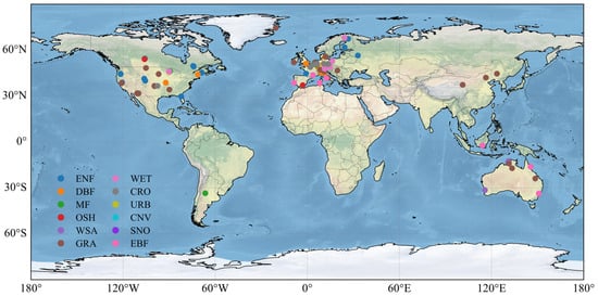
Figure 1.
Geographical distribution of FLUXNET sites based on IGBP classification.
2.3. Experimental Design
The experimental setup was designed for single-point (offline) simulations at each of the 105 FLUXNET sites. The atmospheric forcing data used in the experiments are derived from site observations within the FLUXNET2015 dataset. This dataset has a temporal resolution of 30 min and includes the following seven variables: near-surface wind speed, temperature, humidity, air pressure, shortwave radiation flux, longwave radiation flux, and precipitation. The experimental setup involved inputting new atmospheric forcing data every 30 min. To minimize the influence of initial conditions, a 50-year spin-up simulation was first conducted for each site by repeatedly cycling the available years of forcing data. This ensured that key model state variables, such as soil moisture and temperature, reached a quasi-equilibrium state. Following the spin-up, a final simulation was run for the entire observational period of each site to generate the ET and GPP flux data used in our analysis.
2.4. Analysis Methods
To evaluate the performance of the LSM in simulating water and carbon fluxes across different temporal scales, this study employs common evaluation metrics, including the Pearson correlation coefficient (R), root mean square error (RMSE), and mean absolute error (MAE). The formulas for calculating R, RMSE, and MAE are given in Equations (1)–(3), respectively [29]. The Pearson correlation coefficient (R) measures the degree of linear correlation between simulated and observed values, ranging from −1 to 1. Values closer to 1 indicate a stronger positive correlation, while values closer to −1 indicate a stronger negative correlation. RMSE and MAE quantify the magnitude of the difference between simulated and observed values. Both RMSE and MAE are non-negative, with values closer to 0 indicating smaller errors and better agreement between simulations and observations [30,31].
where xi and yi represent the observed and simulated values, respectively,
x and y are the mean values of observations and simulations, and n is the number of data points.
3. Results and Discussion
3.1. Annual Scale
3.1.1. Evapotranspiration (ET)
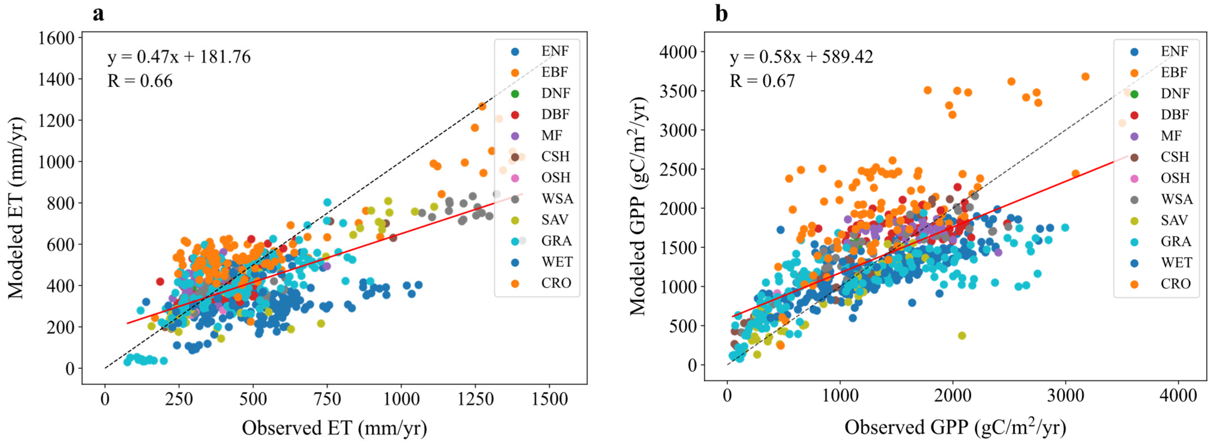
As shown in Table 2 and Figure 2a, the model generally underestimates annual mean ET. The overall simulated annual mean ET is 405.39 mm yr−1, compared to the observed mean of 476.67 mm yr−1, resulting in an absolute error of 71.28 mm yr−1 and a relative error of 14.95%. The overall correlation coefficient (R) is 0.66, indicating a moderate positive linear relationship, but the RMSE of 188.99 mm yr−1 suggests considerable spread. With the exception of DBF, MF, CSH, and CRO, the simulated values are lower than the observations for most vegetation types. The largest underestimation occurs for ENF, with a relative error of 33.26%. This bias may arise from inadequate representation of vegetation transpiration processes, potentially linked to errors in the parameterization of canopy radiation scattering, canopy interception, or the rooting depth of plants [32].
Table 2.
Quantitative evaluation of annual ET simulations against FLUXNET observations across 12 vegetation types defined in Section 2.2.
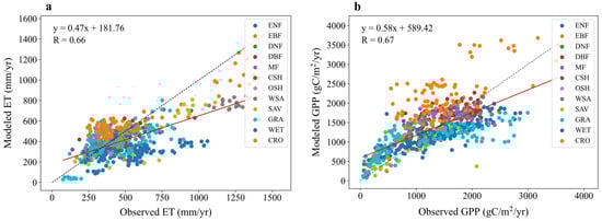
Figure 2.
Comparison of modeled versus observed annual mean for (a) evapotranspiration (ET) and (b) gross primary productivity (GPP) fluxes across 12 vegetation types. Dashed lines indicate a 1:1 relationship, and solid lines show linear regression fits, with correlation coefficients (R) displayed.
Performance varies significantly across vegetation types. CSH shows the best performance with a high correlation (R = 0.93, p < 0.001) and low relative error (6.02%), indicating excellent agreement. DNF performs the worst, with a negative correlation (R = −0.37, p = 0.7555, not significant), significant overestimation (observed 302.13 mm yr−1 vs. simulated 396.04 mm yr−1, relative error 31.08%), and high variability. The lack of significance for OSH (p = 0.545) and DNF might be due to small sample sizes. For most other types (DBF, CSH, WSA, SAV, GRA, WET, CRO), the p-values are <0.001, indicating statistically significant confidence levels.
The significant underestimation of ET in ENF, with a relative error of 33.26%, likely stems from inaccuracies in the LAI simulations for ENF by the default Dynamic Vegetation (DVEG) module within the Noah-MP model. As a critical parameter governing canopy transpiration and interception, biases in DVEG’s LAI simulations are directly propagated into the ET estimates. Moreover, ENFs are characterized by complex canopy structures. Deficiencies in the model’s simulation of intra-canopy radiation transfer (specifically under RAD option 1, a three-dimensional canopy morphology scheme) and energy partitioning may further contribute to the underestimation of both canopy interception evaporation and vegetation transpiration [33].
Conversely, ET simulations for CSH exhibited the highest accuracy. This suggests that either the default Noah-MP parameters (e.g., vegetation physiological parameters, root distribution assumptions) and the DVEG module adequately represent the growth and water use strategies of CSH vegetation, or that the climatic and soil conditions at the selected CSH sites align well with the model’s generalized assumptions. In stark contrast, ET simulations for DNF were the least accurate, marked by significant overestimation and a negative correlation coefficient. This poor performance is largely attributable to an extremely small sample size (only 3 site-years, as indicated in Table 2), rendering the evaluation results highly susceptible to individual anomalous sites or short-term climatic fluctuations and, consequently, compromising the robustness of these findings [34].
3.1.2. Gross Primary Productivity (GPP)
As shown in Table 3 and Figure 2b, the model generally overestimates annual mean GPP. The overall simulated annual mean GPP is 1346.85 gC·m−2·yr−1, compared to the observed mean of 1295.48 gC·m−2·yr−1, resulting in an absolute error of 51.37 gC·m−2·yr−1 and a relative error of 3.97%. The overall correlation coefficient (R) is 0.67, indicating a moderate positive relationship, but the RMSE of 500.62 gC·m−2·yr−1 suggests substantial scatter. Except for ENF, SAV, and GRA, simulated values are higher than observations for most other vegetation types. The largest overestimation occurs for OSH, with a relative error of 53.99%.
Table 3.
Quantitative evaluation of annual GPP simulations against FLUXNET observations across 12 vegetation types defined in Section 2.2.
Among vegetation types, CSH shows the best correlation (R = 0.97, p < 0.001), indicating strong agreement, although the bias is relatively large (absolute error 184.99 gC·m−2·yr−1, relative error 20.06%). OSH performs the worst with a negative correlation (R = −0.72, p = 0.2793, not significant) and significant overestimation (observed 472.18 gC·m−2·yr−1 vs. simulated 727.10 gC·m−2·yr−1), possibly due to inadequate simulation of vegetation transpiration processes in arid regions. The lack of significance for OSH and DNF (p = 0.9428) might again be due to small sample sizes. For ENF, EBF, CSH, WSA, SAV, GRA, WET, and CRO, the p-values are <0.001, indicating statistically significant results.
The overestimation of annual GPP may originate from the simplified parameterization in Noah-MP’s photosynthesis module, particularly its treatment of photosynthetic capacity metrics. While the model employs the Farquhar biochemical framework [35], its reliance on static lookup tables for key parameters, such as the maximum carboxylation rate (Vcmax) and the maximum electron transport rate (Jmax), introduces critical limitations. However, plant photosynthetic capacity exhibits considerable variability across species, within species, and even among different leaves of the same individual; it also undergoes dynamic adjustments in response to environmental conditions (e.g., light availability, temperature, moisture, CO2 concentration, nutrient status) and leaf age [36]. Consequently, if the model’s preset average values for Vcmax or Jmax for a given PFT are systematically higher than the actual photosynthetic capacity of that PFT in specific regions or during particular years, this directly leads to an overestimation of the potential photosynthetic rate. This, in turn, can accumulate, resulting in an overestimation of annual GPP.
3.2. Monthly Scale
3.2.1. Evapotranspiration (ET)
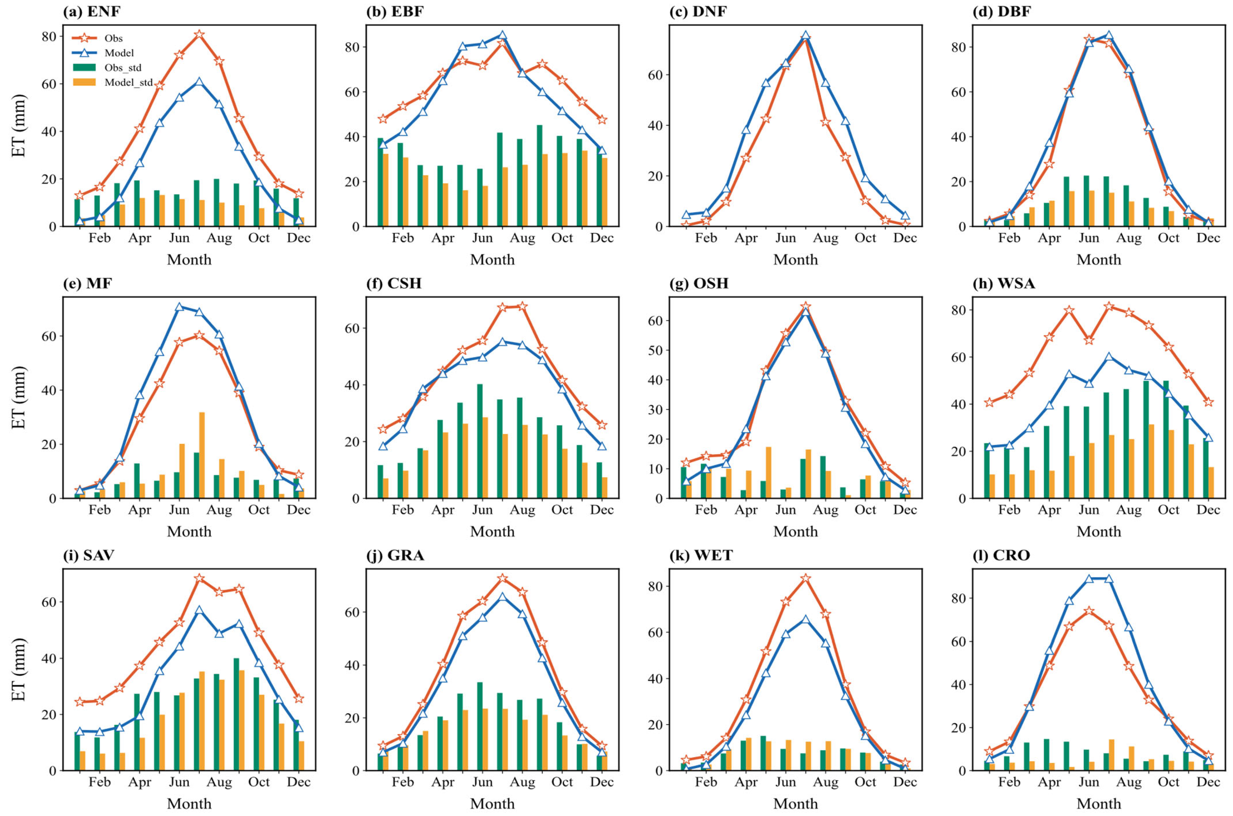
Figure 3 illustrates the multi-year average seasonal cycle of simulated and observed monthly ET, along with the standard deviation across sites for each month. The model generally captures the monthly variation well. Most vegetation types exhibit a “single-peak” seasonal distribution (seasons defined by the Northern Hemisphere: Spring MAM, Summer JJA, Autumn SON, Winter DJF; the Southern Hemisphere shifted by 6 months), with peaks typically occurring in summer (June–August) and troughs in winter (December–February). The simulated seasonal fluctuations align reasonably well with the observations, suggesting the model responds appropriately to the seasonal dynamics of climate drivers (mainly radiation, temperature, and precipitation).

Figure 3.
Multiyear averaged seasonal variations (solid lines) in the simulated and observed ET flux across 12 vegetation types and the corresponding standard deviation (bar charts) across sites: (a) ENF: evergreen needleleaf forest; (b) EBF: evergreen broadleaf forest; (c) DNF: deciduous needleleaf forest; (d) DBF: deciduous broadleaf forest; (e) MF: mixed forest; (f) CSH: closed shrublands; (g) OSH: open shrublands; (h) WSA: woody savanna; (i) SAV: savanna; (j) GRA: grasslands; (k) WET: wetlands; (l) CRO: croplands.
However, for many vegetation types (e.g., WSA, CRO, and ENF), the simulation bias for summer ET is generally larger than for winter ET. This indicates that the model’s ability to capture inter-site ET heterogeneity decreases during seasons with high energy input, leading to greater uncertainty under high radiation and strong transpiration conditions. The standard deviation (represented by bar height in Figure 3) also shows seasonal differences. For most types, the standard deviation among sites is larger in summer than in winter, implying greater variation in simulation performance across different locations during the peak growing season. EBF is an exception, showing larger standard deviation in winter.
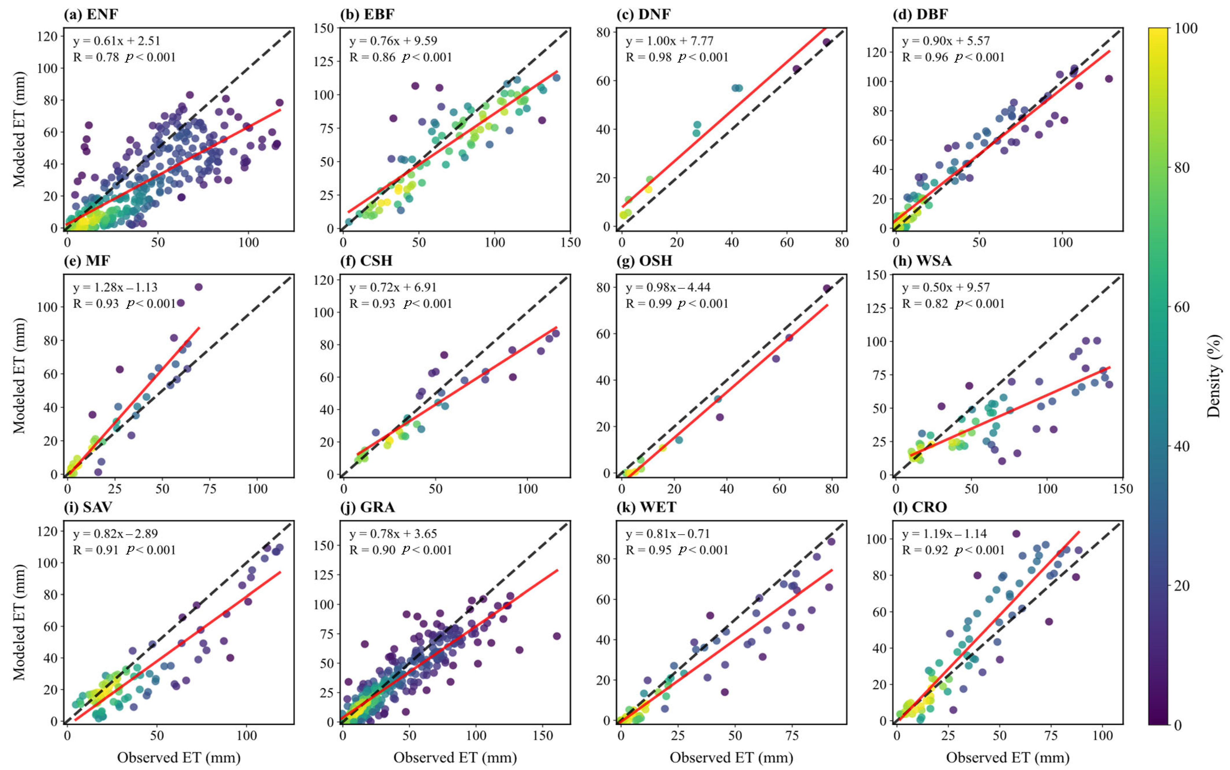
Figure 4 presents scatter plots comparing simulated and observed monthly mean ET across sites for each vegetation type. The correlation for seasonal ET variation is generally high, with R values above 0.8 (often >0.9) for all vegetation types except ENF. For OSH and WSA, simulated monthly means are consistently lower than observed means (points below the 1:1 line). Conversely, for WET and MF, simulated values are significantly higher than observed values (points above the 1:1 line), suggesting overestimation in high-humidity or complex vegetation structure environments.
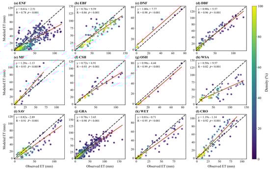
Figure 4.
Scatter plots of monthly ET flux between simulation and observation for sites in different vegetation types: (a) ENF; (b) EBF; (c) DNF; (d) DBF; (e) MF; (f) CSH; (g) OSH; (h) WSA; (i) SAV; (j) GRA; (k) WET; (l) CRO. Dashed lines indicate a 1:1 relationship, and solid lines show linear regression fits, with correlation coefficients (R) displayed.
3.2.2. Gross Primary Productivity (GPP)
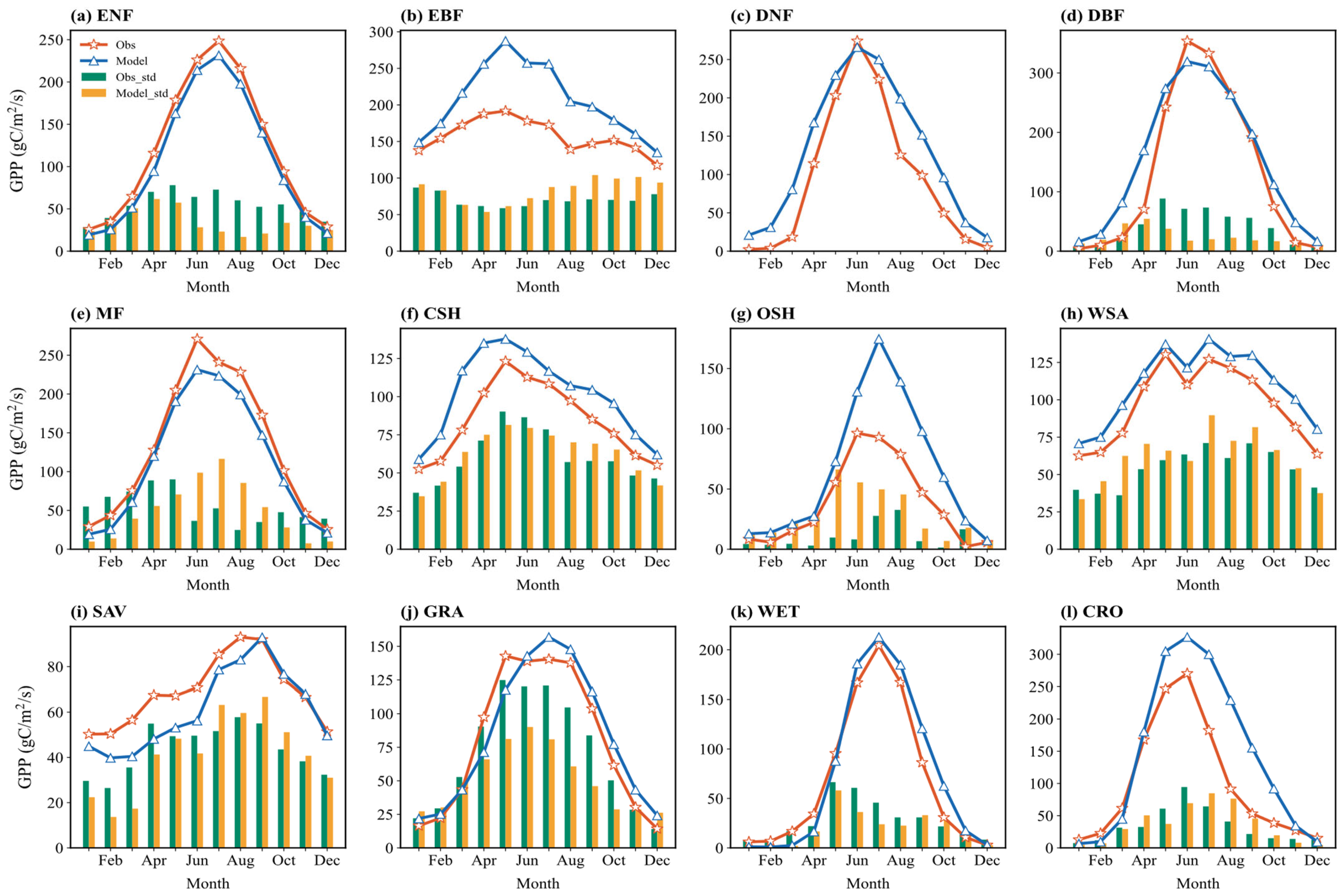
Figure 5 shows the multi-year average seasonal cycle of simulated and observed monthly GPP and its standard deviation across sites. Simulated and observed GPP generally show good agreement in seasonal variations for most vegetation types, exhibiting single-peak or double-peak structures. Peaks typically occur during the growing season (summer, June–August), and troughs during the non-growing season (winter, December–February). For example, in ENF, both the simulated and observed GPP remain high from May to September, peaking in July, reflecting the model’s ability to capture the year-round photosynthetic activity of needleleaf forests.
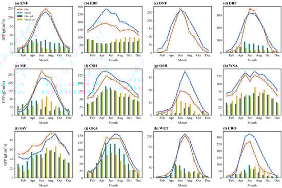
Figure 5.
Multiyear averaged seasonal variations (solid lines) in the simulated and observed GPP flux across 12 vegetation types and the corresponding standard deviation (bar charts) across sites: (a) ENF; (b) EBF; (c) DNF; (d) DBF; (e) MF; (f) CSH; (g) OSH; (h) WSA; (i) SAV; (j) GRA; (k) WET; (l) CRO.
The bar charts in Figure 5 indicate that the seasonal distribution of multi-site standard deviation varies among vegetation types. For GRA, the standard deviation is significantly higher in summer (June–August) than in winter (December–February), suggesting greater variability in simulation results among different grassland sites during the peak growing season. Conversely, for CRO, the standard deviation is relatively low throughout the year, indicating high consistency in GPP simulation across cropland sites, possibly related to simplified representations of management practices like irrigation and fertilization.
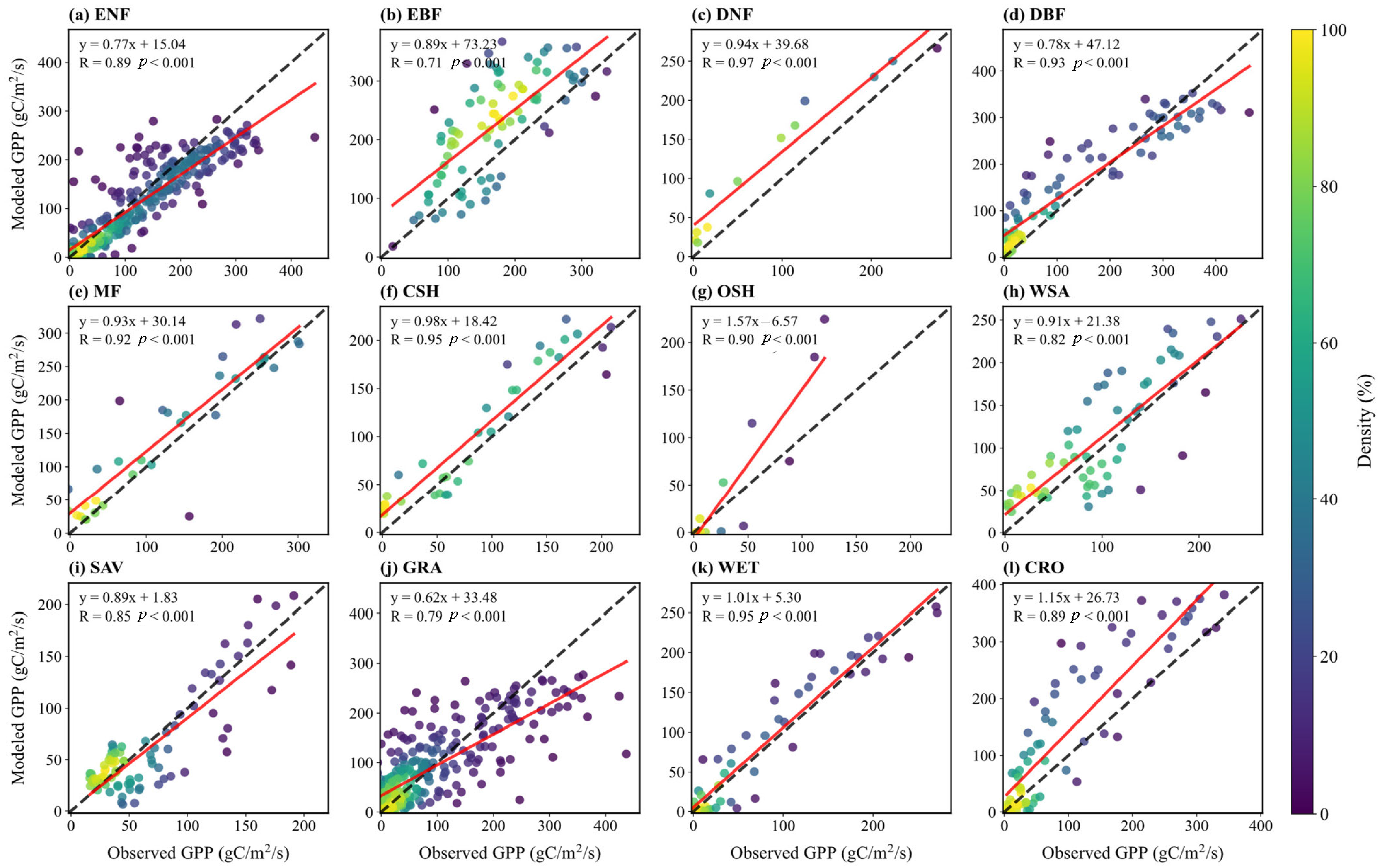
Figure 6 displays scatter plots comparing simulated and observed multi-year monthly mean GPP across sites. The model shows high correlation between simulated and observed GPP for different vegetation types (R values range from 0.71 to 0.97, all p < 0.001), indicating that simulations effectively capture the GPP flux trends. Except for EBF and GRA, R values are above 0.8 for all other types. For WET, the scatter points cluster closely around the 1:1 line, with a high correlation (R = 0.95). Forest ecosystems (ENF, DNF, DBF, etc.) generally show high correlations (R ≥ 0.89), while GRA and WSA exhibit weaker performance (R = 0.79, 0.82), potentially underestimating the dynamic response of herbaceous vegetation to environmental forcing like water limitation.
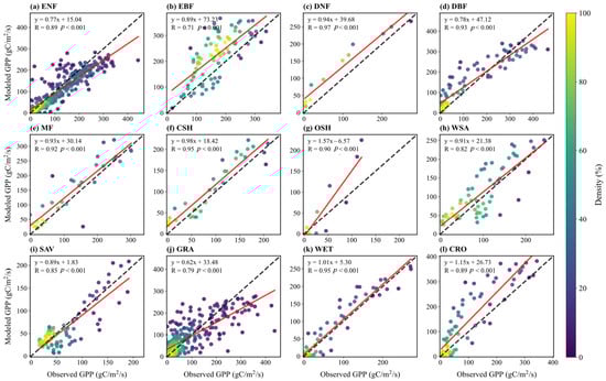
Figure 6.
Scatter plots of monthly GPP flux between simulation and observation for sites in different vegetation types: (a) ENF; (b) EBF; (c) DNF; (d) DBF; (e) MF; (f) CSH; (g) OSH; (h) WSA; (i) SAV; (j) GRA; (k) WET; (l) CRO. Dashed lines indicate a 1:1 relationship, and solid lines show linear regression fits, with correlation coefficients (R) displayed.
3.3. Diurnal Variation
3.3.1. Evapotranspiration (ET)
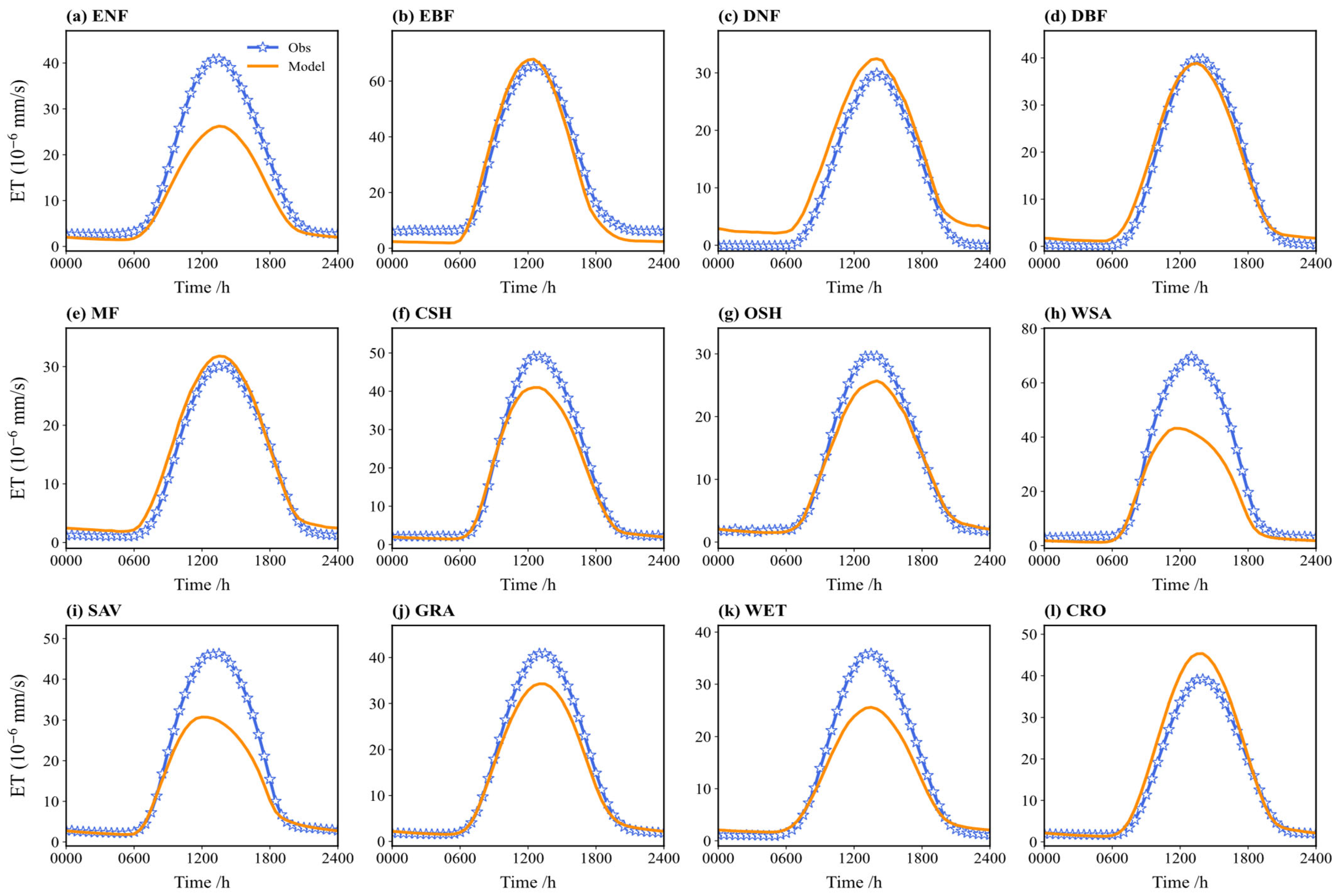
Figure 7 compares the multi-year average diurnal cycle of simulated and observed ET. The simulated and observed diurnal cycles are mostly consistent, both showing a “single-peak” structure peaking around noon (local time 12:00), characteristic of solar radiation-driven evapotranspiration. For several vegetation types (e.g., ENF, WSA, WET, SAV), the simulated values during daytime (especially 12:00–14:00) are significantly lower than the observed values. For ENF, the noon underestimation can reach 10–15%. Conversely, for CRO and MF, the simulated values exceed the observations during parts of the day; for CRO, around 14:00, the simulations are 5–8% higher. Nighttime ET is minimal in both the simulations and observations, with little discrepancy.
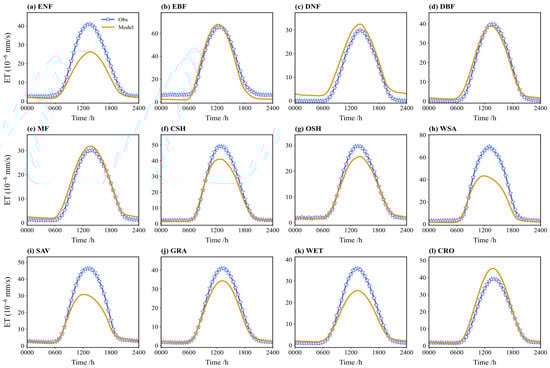
Figure 7.
Comparison between the observed and simulated ET flux on a diurnal course in different vegetation types (multi-year average): (a) ENF; (b) EBF; (c) DNF; (d) DBF; (e) MF; (f) CSH; (g) OSH; (h) WSA; (i) SAV; (j) GRA; (k) WET; (l) CRO.
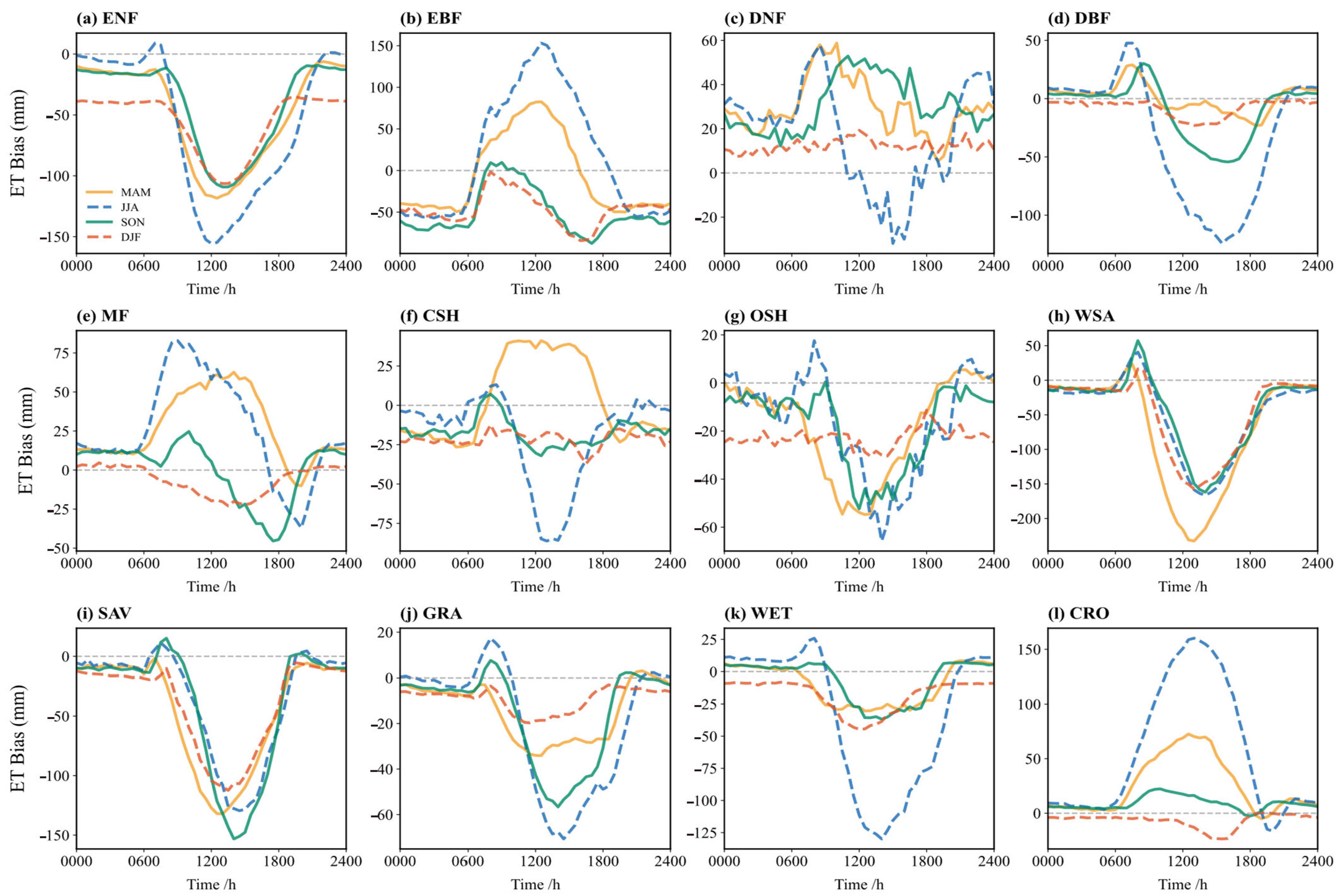
Figure 8 shows the diurnal cycle of simulation bias (simulation minus observation) for ET across different seasons. Overall, the simulation biases are significantly larger during the summer under high temperature and radiation conditions. Winter simulations perform best, while spring and autumn are intermediate. Summer (JJA) exhibits the largest biases, with midday deviations amplified 2–3 times compared to winter (DJF), reaching up to 160 mm. This suggests challenges in simulating complex vegetation physiological and soil moisture processes under high-temperature, high-radiation conditions. In winter, the biases are generally small for all vegetation types, with bias curves close to zero, indicating good agreement. The simplified ET processes during low temperatures, dominated by basic physics, like soil heat conduction and vegetation dormancy, appear well-captured. During the summer midday, the model tends to overestimate ET for EBF, DNF, MF, and CSH, while underestimating it for other vegetation types.
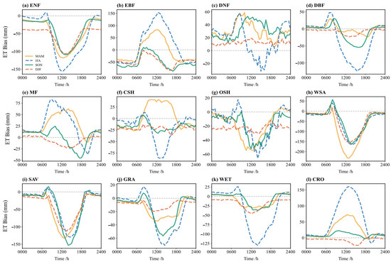
Figure 8.
Bias (simulation minus observation) of the multi-year average diurnal variation of ET flux in different vegetation types in spring, summer, autumn, and winter: (a) ENF; (b) EBF; (c) DNF; (d) DBF; (e) MF; (f) CSH; (g) OSH; (h) WSA; (i) SAV; (j) GRA; (k) WET; (l) CRO.
3.3.2. Gross Primary Productivity (GPP)
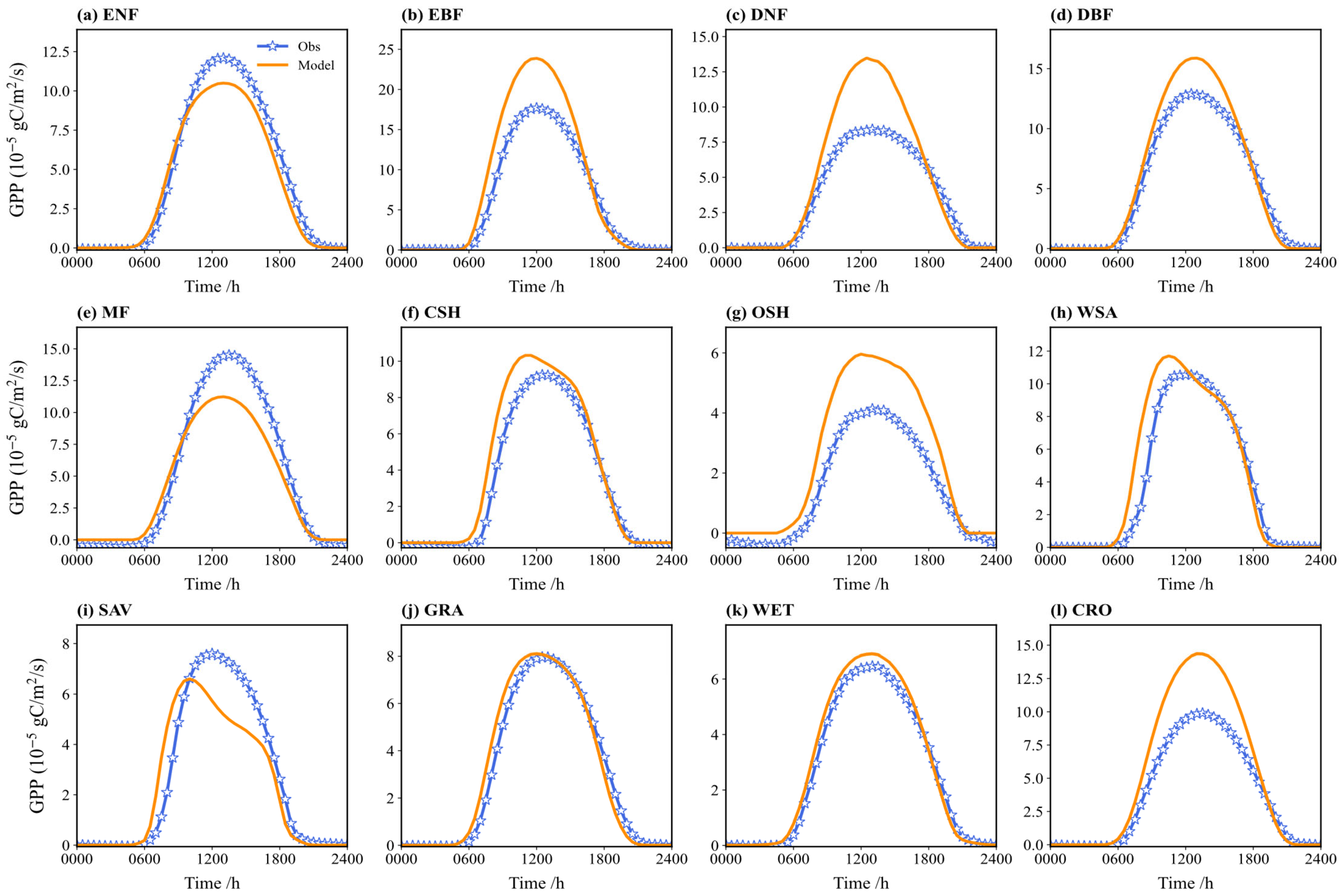
Figure 9 compares the multi-year average diurnal cycle of simulated and observed GPP. The diurnal patterns are generally consistent, showing a distinct “single-peak” around noon (local time 12:00), aligning with the typical diurnal pattern of photosynthesis. During the daytime (06:00 to 18:00), simulated GPP is underestimated to varying degrees for vegetation types like EBF, DNF, CSH, and OSH. Conversely, the simulations tend to overestimate GPP for MF, SAV, and ENF. The simulations for GRA and WET show the closest agreement with the observations. Nighttime GPP is near zero in both the simulations and observations for most types.
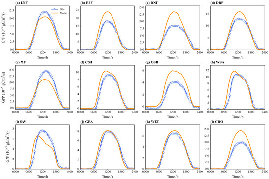
Figure 9.
Comparison between the observed and simulated GPP flux on a diurnal course in different vegetation types (multi-year average): (a) ENF; (b) EBF; (c) DNF; (d) DBF; (e) MF; (f) CSH; (g) OSH; (h) WSA; (i) SAV; (j) GRA; (k) WET; (l) CRO.
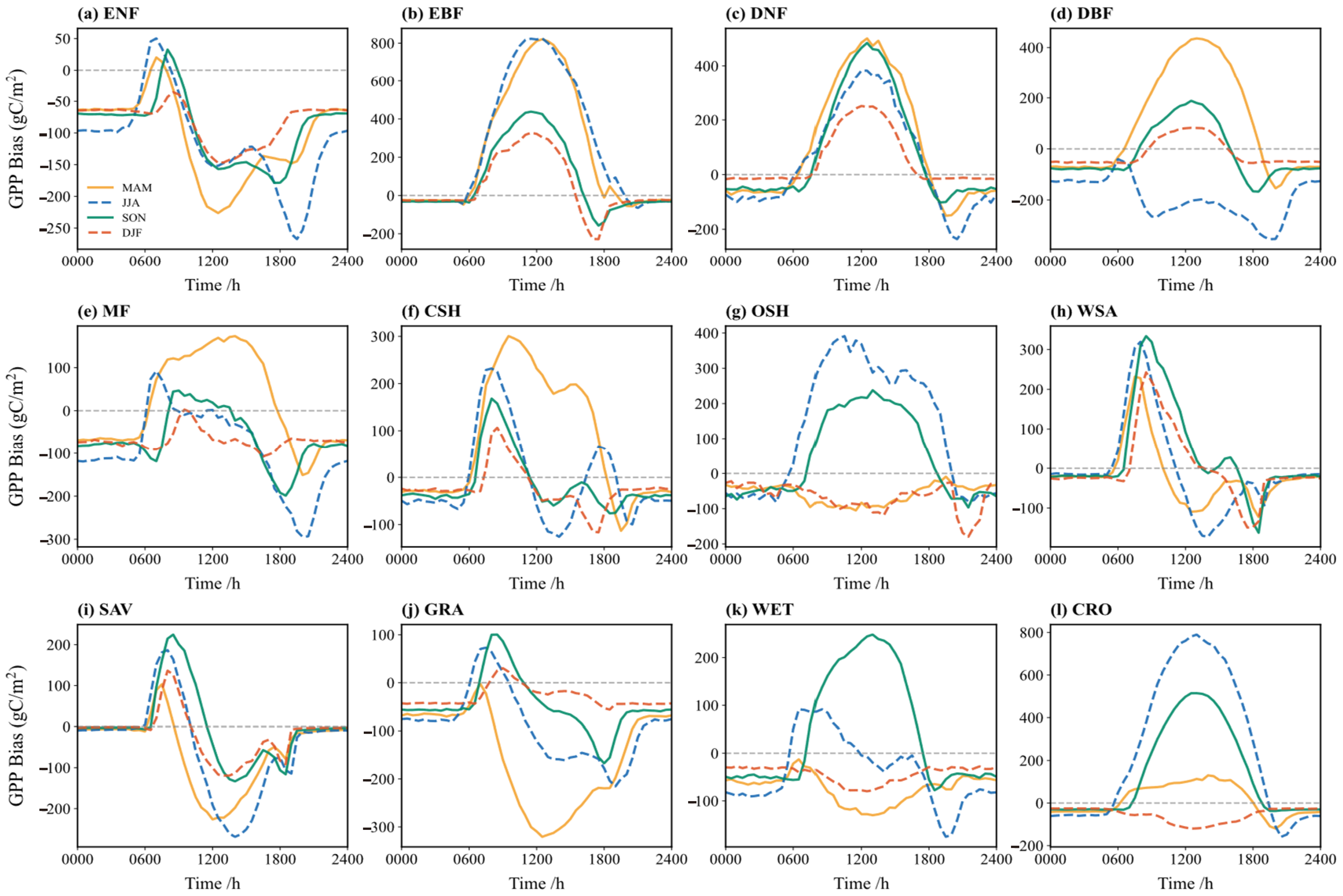
Figure 10 illustrates the diurnal cycle of GPP simulation bias across the seasons. Diurnal biases are larger in the spring and summer, potentially reaching 800 gC/m2, whereas autumn and winter biases are mostly within 200 gC/m2. For vegetation types like ENF, CSH, SAV, GRA, and WET, the simulated GPP is higher than observed in the early morning during the summer (positive bias), but the bias fluctuates complexly after noon, possibly due to photoinhibition or other physiological processes. In the winter, when vegetation activity is reduced, biases are relatively stable and smaller.
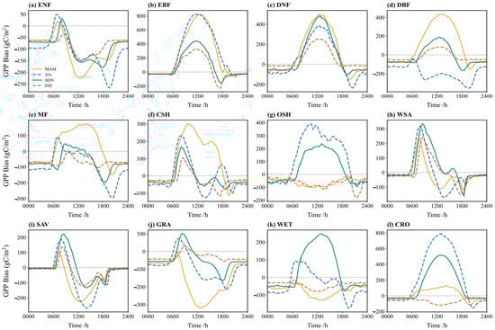
Figure 10.
Bias (simulation minus observation) of the multi-year average diurnal variation of GPP flux in different vegetation types in spring (yellow), summer (blue), autumn (green), and winter (red): (a) ENF; (b) EBF; (c) DNF; (d) DBF; (e) MF; (f) CSH; (g) OSH; (h) WSA; (i) SAV; (j) GRA; (k) WET; (l) CRO.
3.4. Comparison of Simulation Performance Across Different Temporal Scales
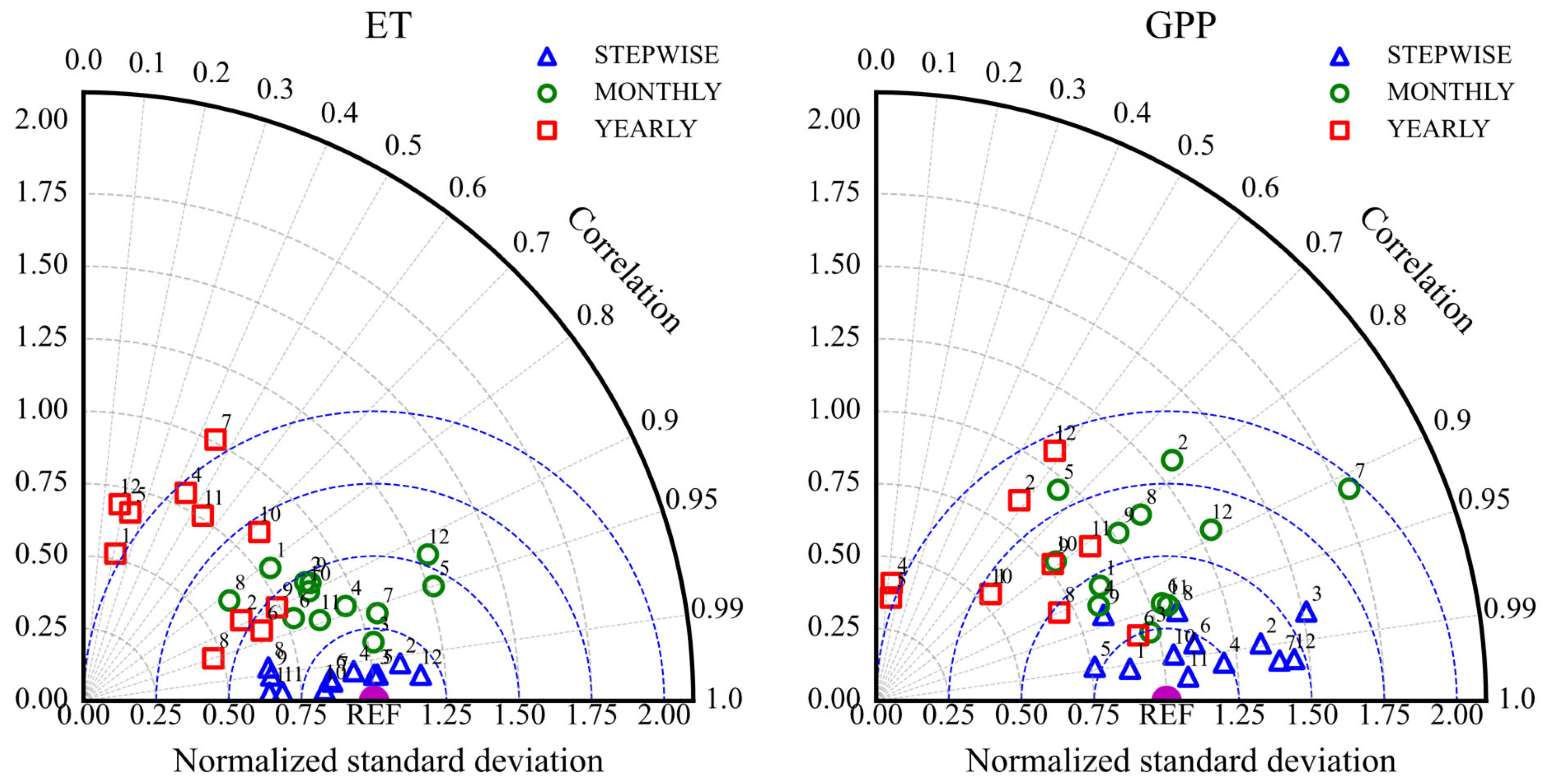
Figure 11 presents a Taylor diagram summarizing the model’s simulation skill for ET and GPP across different temporal scales (half-hourly, monthly, annual) based on the Pearson correlation coefficient (R) and standardized deviation (SD). The R values for water and carbon fluxes mainly range from 0.6 to 1 (ET) and 0.5 to 1 (GPP), while SD values range from 0.5 to 1.3 and 0.5 to 1.5, respectively.
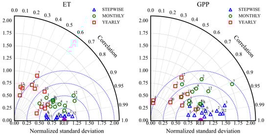
Figure 11.
Taylor diagram showing the comparison of simulation performance for ET and GPP at half-hourly, monthly, and annual temporal scales for different vegetation types (1: ENF; 2: EBF; 3: DNF; 4: DBF; 5: MF; 6: CSH; 7: OSH; 8: WSA; 9: SAV; 10: GRA; 11: WET; 12: CRO).
The model simulations for both ET and GPP show high consistency with observations at the half-hourly scale, with R values typically between 0.8 and 1. The ET simulations also maintain good consistency at the monthly scale, with R values mostly between 0.95 and 1. At the annual scale, the GPP simulations show correlations above 0.5 for most vegetation types, except for DNF, DBF, MF, and OSH, which did not pass the significance tests. Figure 12 also indicates that annual scale simulation biases (RMSE and MAE) are relatively small in magnitude compared to the total annual flux, despite lower correlations.
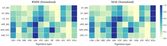
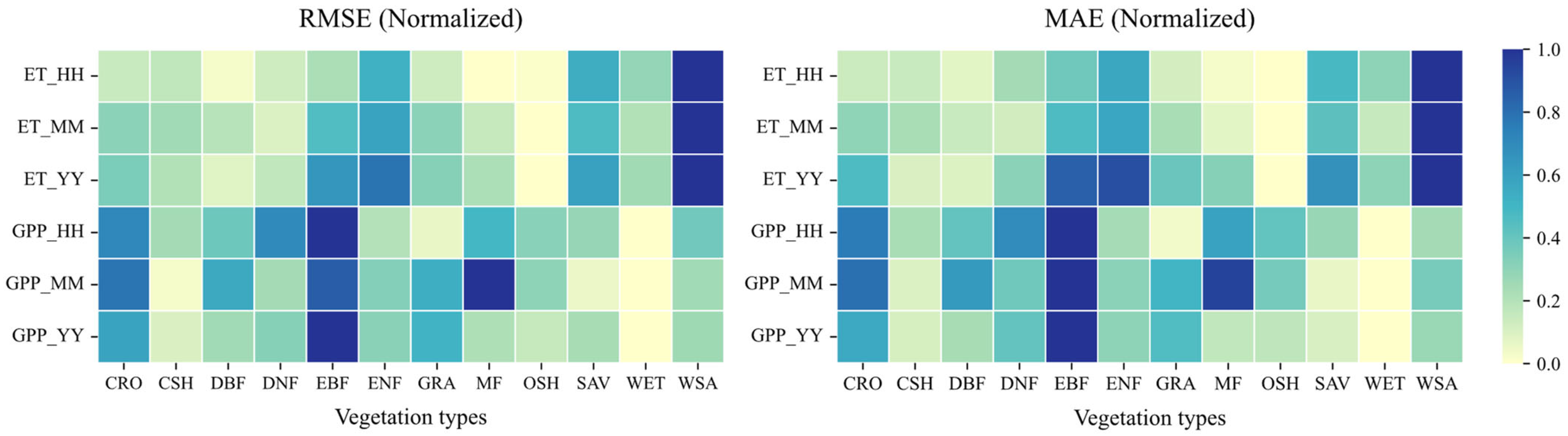
Figure 12.
Model performance in simulating ET and GPP on temporal scales of half-hourly (HH), monthly (MM), and annual (YY) measured using the RMSE and MAE for different vegetation types.
Overall, RMSE and MAE values (Figure 12) are smallest at the half-hourly scale and largest at the annual scale. This reflects that the model has the smallest simulation bias at the half-hourly scale, performing better than at monthly or annual scales in terms of absolute error magnitude relative to the variability at that scale. Comparing ET and GPP (Figure 11), the model generally performs better for ET than for GPP. At half-hourly and monthly scales, the ET simulations show higher R values and SD values closer to the reference point (REF = 1) compared to GPP. Furthermore, Figure 12 shows that the average RMSE and MAE values for ET across all three temporal scales are smaller than those for GPP.
Noah-MP 5.0’s simulation accuracy for ET and GPP is significantly higher at the half-hourly scale compared to the annual scale (ET: R = 0.93 vs. 0.66; GPP: R = 0.89 vs. 0.67). This aligns with the model’s ability to finely capture responses to transient drivers like radiation and temperature at short temporal scales. However, the substantial increase in cumulative error at the annual scale highlights the deficiencies in simulating long-term cumulative effects of vegetation physiology, such as carbon allocation and soil moisture memory. Silva et al. [37] observed similar phenomena in tropical rainforest evaluations, suggesting that the parameterization of phenological lag responses in Noah-MP’s dynamic vegetation module requires further optimization.
3.5. Comparison of Simulation Performance Across Climate Zones
To investigate the influence of background climate on model fidelity, a climate-stratified evaluation was performed. The 105 FLUXNET sites were categorized based on the globally recognized Köppen–Geiger climate classification system, which delineates climate zones according to the distinct seasonal patterns of temperature and precipitation [38]. For this analysis, sites were aggregated into five principal climate regions: Tropical, Arid, Temperate, Continental, and Polar. The model’s performance in simulating annual ET and GPP within each zone is quantitatively presented in Table 4 and Table 5, with the distribution of simulation biases visualized in Figure 13.
Table 4.
Quantitative evaluation of annual ET simulations against FLUXNET observations across climate zone.
Table 5.
Quantitative evaluation of annual GPP simulations against FLUXNET observations across climate zone.
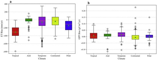
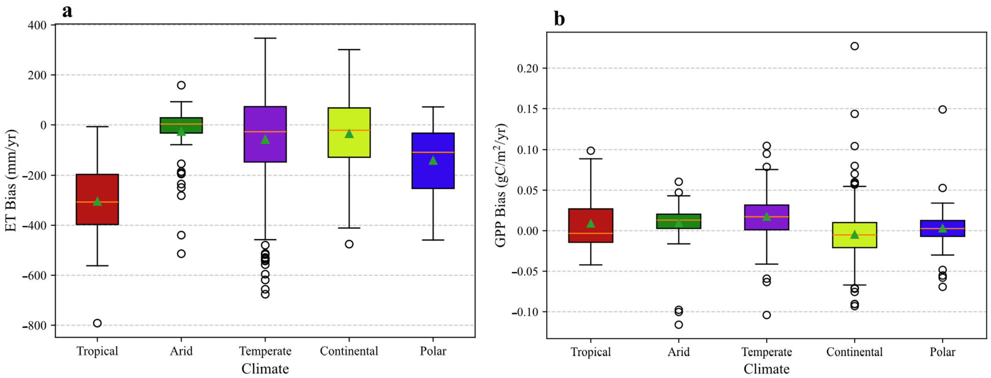
Figure 13.
Distribution of annual simulation biases for (a) evapotranspiration (ET) and (b) gross primary productivity (GPP) across five principal climate zones. The bias is calculated as the simulated value minus the observed value. In the box plot, the central horizontal line indicates the median, while the bottom and top edges of the box represent the 25th (Q1) and 75th (Q3) percentiles, respectively. The whiskers extend to the most extreme data points within 1.5 × IQR (where IQR = Q3 − Q1) of the box. The triangle symbol (△) indicates the mean value. Individual points beyond the whiskers are marked as outliers.
3.5.1. Evapotranspiration (ET)
The model’s simulation of ET exhibits a pronounced, climate-dependent error structure. A general tendency to overestimate annual ET is evident, with the largest mean positive biases occurring in the Polar and Tropical regions. Conversely, the Arid zone displays the smallest mean deviation.
Of particular significance is the model’s apparent incapacity to capture the inter-annual variability of ET in mid-latitude climates. In both the Temperate and Continental zones, the correlation between simulated and observed annual ET is statistically insignificant. This finding suggests a fundamental deficiency in the model’s ability to represent the drivers of hydrological dynamics in these regions, limiting its utility for climate sensitivity and trend analyses. The underlying cause may be linked to an inadequate parameterization of the processes critical to these climates, such as snowmelt hydrology, soil freeze–thaw dynamics, and vegetation phenological controls on canopy conductance [39,40].
The distribution of simulation biases further elucidates performance heterogeneity (Figure 13a). In the Tropical zone, a notable divergence exists between the mean bias, which indicates a strong overestimation, and the median bias, which suggests an underestimation of approximately 300 mm yr−1. This implies that the arithmetic mean is highly skewed by extreme positive errors at a subset of sites, while the model’s typical behavior is to underestimate ET. The broad interquartile ranges observed in the Temperate and Continental zones signify substantial simulation uncertainty and low model robustness across the sites within these regions.
3.5.2. Gross Primary Productivity (GPP)
In contrast to ET, the GPP simulations demonstrated statistically significant positive correlations with the observations across all five climate regions (p < 0.01 for all). However, the model’s ability to capture the correct magnitude and variability of GPP is highly climate-dependent.
The model systematically overestimates GPP, a bias most pronounced in the Arid (53.11%) and Temperate (+26.80%) zones. In the Arid zone, the large positive mean bias contrasts with a near-zero median bias (Figure 13b), indicating that extreme overestimation at a subset of sites skews the average. This suggests a conditionally flawed water-stress parameterization that inadequately suppresses photosynthesis during drought [41,42,43]. The consistent overestimation in the Temperate zone, reflected by its positive median bias and wide interquartile range, points to an overly optimistic parameterization of photosynthetic capacity (e.g., Vcmax) within the model’s PFT scheme, possibly compounded by phenological inaccuracies [44,45].
Furthermore, the fidelity with which the model captures GPP variability is low in climates with complex, interacting limiting factors. The correlation is notably poor in the Arid (R = 0.31) and Continental (R = 0.24) zones. The Continental region is unique in exhibiting a mean GPP underestimation (−6.99%). Visually, its box plot in Figure 13b displays the largest interquartile range among all climates, indicating the highest degree of simulation uncertainty. This high site-to-site variability, coupled with the very weak correlation, underscores the model’s struggle to consistently simulate physiological responses to the wide temperature extremes of this climate. This could involve over-penalizing productivity during summer heat stress while inaccurately modeling the rapid onset of photosynthesis following cold-period dormancy [46,47].
By contrast, the stronger correlations in the Tropical (R = 0.74) and Polar (R = 0.74) zones, supported by the more compact and centered bias distributions in Figure 13b, suggest greater model skill where GPP dynamics are governed by a single, dominant environmental driver, such as radiation or a temperature-defined growing season.
4. Discussion
4.1. Discrepancies in Model Capability Across Temporal Scales
The model performs best at short temporal scales (e.g., half-hourly), but its performance deteriorates as the temporal resolution increases to monthly and annual scales, due to the accumulation of systematic errors. This highlights the model’s varying capacity to represent processes across different time scales, which primarily stems from its differential ability to characterize dominant processes and transmit the “memory effect” of slow variables.
At sub-daily to daily scales, fluxes are primarily driven by immediate atmospheric forcing and rapid physical and physiological responses of the vegetation canopy and upper soil layers. These processes are generally well-represented in Noah-MP through established physical laws and biochemical equations [17].
However, at longer time scales (e.g., monthly, seasonal, or annual), system memory becomes increasingly important—meaning that current flux states are not only influenced by the immediate forcings, but by the accumulated conditions of slow variables over time, such as deep soil moisture, vegetation biomass, and LAI. Noah-MP’s simulation of these slow processes often relies on empirical parameters, simplified assumptions, and limited representation of complex feedbacks. These structural uncertainties, coupled with imperfect coupling among model components, contribute to the accumulation and amplification of short-term biases over time [48,49,50].
4.2. Challenges in Simulating Complex and Heterogeneous Canopies
The model exhibits significant biases in ecosystems with complex canopy structures and heterogeneous compositions, revealing limitations in its underlying assumptions.
The consistent underestimation of ET in ENF points to deficiencies in the model’s radiation transfer scheme. Noah-MP’s default single-layer, “big-leaf” approach treats the canopy as a single, homogenous entity. This simplification fails to capture the intricate three-dimensional structure of dense, multi-layered coniferous canopies. It cannot adequately represent processes like self-shading or the vertical gradients in light and microclimatic within the canopy. Consequently, the contribution of lower, shaded parts of the canopy to total ecosystem transpiration is likely underestimated, leading to a systematic low bias in total ET.
The poor performance in WSA highlights the model’s difficulty in simulating resource competition between different PFTs within a single grid cell. Savannas are composed of co-existing trees and grasses, which compete for light, water, and nutrients. These life forms have different rooting depths, phenological timings, and physiological responses to stress. A single-grid-cell model, like Noah-MP, struggles to resolve this sub-grid heterogeneity, particularly the asymmetric competition for soil water between deep-rooted trees and shallow-rooted grasses. Inaccuracies in partitioning these resources lead to significant errors in the simulated water and carbon fluxes for the ecosystem as a whole [51,52].
4.3. The “Midday Depression” Simulation Gap
At the diurnal scale, the largest simulation biases for both ET and GPP frequently occur around noon, especially during summer. This points to a gap in the model’s ability to simulate plant responses to combined high-stress conditions (i.e., high vapor pressure deficit (VPD) and high radiation). The observed underestimation of ET in many PFTs during midday suggests that the stomatal conductance model may be overly sensitive, predicting a more pronounced stomatal closure (“midday depression”) than what occurs in reality. Conversely, overestimated GPP at noon in other types indicates the model may not be fully accounting for protective mechanisms, like non-photochemical quenching (NPQ) or direct heat stress on enzymatic activity, which down-regulate photosynthesis under peak stress [36].
4.4. Limitations
A fundamental source of uncertainty in this study stems from the atmospheric forcing data utilized to drive the model simulations. We employed the standardized FLUXNET2015 dataset, a composite product where gaps in in situ meteorological observations are filled with downscaled data from the ECMWF reanalysis. While this procedure is essential for creating the complete and continuous time series required for land surface model simulations, it inevitably introduces a degree of uncertainty. These potential discrepancies arise from two primary sources, including (1) the spatial scale mismatch between the coarse-resolution reanalysis grid and the point-scale flux tower footprint, and (2) the inherent systematic biases within the reanalysis model itself. Consequently, a portion of the model-data error reported herein must be attributed to this forcing uncertainty. This is particularly relevant for variables like precipitation, where errors in timing and intensity can propagate directly into the simulation of soil moisture dynamics and, subsequently, the surface fluxes of water and carbon. Quantitatively partitioning the total simulation error between forcing data uncertainty and model structural deficiencies is a persistent challenge in the field of land surface modeling, and remains beyond the scope of this evaluation [53,54].
Furthermore, the geographical distribution of the FLUXNET sites is imbalanced, leading to insufficient ecological representation. The 105 selected sites are primarily concentrated in western Europe and north America, with a significant lack of coverage in tropical rainforests like the Amazon and southeast Asia, and cold regions such as Siberia and the Tibetan Plateau. This uneven distribution may limit the comprehensive evaluation of the model’s adaptability to high-radiation, high-humidity, or extreme low-temperature environments. Recent studies underscore that tropical ecosystem environments present unique modeling challenges that differ substantially from temperate systems. For instance, research in seasonally dry tropical forests and in the Amazon rainforest has highlighted the critical role of deep rooting systems, plant hydraulic strategies, and complex phenological responses to seasonal water availability in controlling land–atmosphere fluxes. Furthermore, studies have demonstrated that standard model parameterizations often fail to capture the resilience of these ecosystems to drought, leading to significant errors in GPP and ET simulations [55,56,57,58]. Additionally, some vegetation types (e.g., DNF and OSH) have very few representative sites or site-years, potentially leading to larger uncertainties and less robust conclusions for those types.
Additionally, our analysis is primarily stratified by vegetation type rather than by background climate. The geographical distribution of the FLUXNET sites means that certain vegetation types are inherently confounded with specific climate zones (e.g., savannas in water-limited regions, certain forests in temperate zones). A dedicated analysis segmented by a climate classification system would be necessary to disentangle the effects of vegetation physiology from those of overarching climatic drivers (e.g., aridity, temperature limitations). Such an investigation would better clarify the model’s structural weaknesses under specific environmental stresses, and remains a critical avenue for future research.
A further limitation is that the model does not account for human activities like irrigation and fertilization in agricultural ecosystems. The absence of agricultural management modules, such as those for irrigation and fertilization, results in significant simulation biases for CRO. This is evidenced by a substantial absolute error of 503.21 gC·m−2·yr−1 and a relative error of 43.31% for GPP in agricultural areas.
Finally, our parameter sensitivity analysis was limited to predefined scheme combinations and did not include parameter optimization experiments. Consequently, while model performance was assessed under existing configurations, we did not explore how fine-tuning specific parameters might improve its accuracy across diverse regions and conditions. Future research could benefit from coupling data assimilation systems with multi-source remote sensing observations (e.g., SMAP, GOSAT) to enhance the regional adaptability of these parameters [59].
5. Conclusions
This study evaluated the Noah-MP land surface model using single-point simulations against observations from 105 FLUXNET2015 sites across 12 typical vegetation types. The performance in simulating ET and GPP was assessed at half-hourly, monthly, and annual temporal scales. The main results were as follows:
- (1)
- Noah-MP generally performed well in simulating ET and GPP fluxes, capturing their variability characteristics with relatively small biases compared to the observations. The ET simulations showed slightly better agreement with the observations than the GPP simulations.
- (2)
- Simulation performance varied significantly with temporal scales, systematically decreasing as the time scale lengthened. At the half-hourly scale, simulated ET and GPP showed high consistency with observations, indicating strong capability in capturing responses to short-term drivers. At the annual scale, cumulative errors increased substantially.
- (3)
- Noah-MP generally captured the characteristic diurnal, seasonal, and interannual variations of ET and GPP. Diurnal simulation biases were often largest around noon. Seasonally, simulation biases for both fluxes were smallest in winter. Inter-site simulation performance showed greater variability during the summer compared to the winter. The standard deviation across sites was smaller for ET than for GPP, suggesting less spread in the ET simulation performance.
- (4)
- Based on the evaluation metrics, the ET simulations performed relatively well for OSH, DBF, and MF, with the largest bias observed for WSA. The GPP simulations performed relatively well for WET, CSH, and SAV, with the largest bias occurring for EBF.
- (5)
- Noah-MP exhibits a strong dependence on the climatic region. For ET, the model fails to capture the inter-annual variability in temperate and continental climates, indicating a fundamental weakness in simulating mid-latitude hydrology. For GPP, the model exhibits severe magnitude biases, particularly as overestimation in arid and temperate zones, while also failing to capture the temporal dynamics in arid and continental climates.
Supplementary Materials
The following supporting information can be downloaded at: https://www.mdpi.com/article/10.3390/land14071400/s1.
Author Contributions
Methodology, B.P. and X.W.; Software, B.P.; Validation, B.P.; Formal analysis, B.P.; Investigation, X.W.; Resources, X.W.; Data curation, X.W.; Writing—original draft, B.P.; Writing—review & editing, X.C.; Visualization, B.P.; Supervision, X.C.; Project administration, X.C.; Funding acquisition, X.C. All authors have read and agreed to the published version of the manuscript.
Funding
This work is supported by the National Key Research and Development Program of China (2023YFF0805501) and the National Natural Science Foundation of China (42375165). We thank the technical support of the National Large Scientific and Technological Infrastructure “Earth System Numerical Simulation Facility” (https://cstr.cn/31134.02.EL (accessed on 1 June 2025)).
Data Availability Statement
The data presented in this study are openly available in FLUXNET at https://fluxnet.org/data/fluxnet2015-dataset (accessed on 3 December 2024).
Conflicts of Interest
The authors declare no conflicts of interest.
References
- Bonan, G.B. Forests and Climate Change: Forcings, Feedbacks, and the Climate Benefits of Forests. Science 2008, 320, 1444–1449. [Google Scholar] [CrossRef]
- Reichstein, M.; Bahn, M.; Ciais, P.; Frank, D.; Mahecha, M.D.; Seneviratne, S.I.; Zscheischler, J.; Beer, C.; Buchmann, N.; Frank, D.C.; et al. Climate Extremes and the Carbon Cycle. Nature 2013, 500, 287–295. [Google Scholar] [CrossRef]
- Gong, K.; Huang, Z.; Qu, M.; He, Z.; Chen, J.; Wang, Z.; Yu, Q.; Feng, H.; He, J. Influences of Climate Change on Carbon and Water Fluxes of the Ecosystem in the Qinling Mountains of China. Ecol. Indic. 2024, 166, 112504. [Google Scholar] [CrossRef]
- Fisher, J.B.; Melton, F.; Middleton, E.; Hain, C.; Anderson, M.; Allen, R.; McCabe, M.F.; Hook, S.; Baldocchi, D.; Townsend, P.A.; et al. The Future of Evapotranspiration: Global Requirements for Ecosystem Functioning, Carbon and Climate Feedbacks, Agricultural Management, and Water Resources. Water Resour. Res. 2017, 53, 2618–2626. [Google Scholar] [CrossRef]
- Xue, B.; A, Y.; Wang, G.; Helman, D.; Sun, G.; Tao, S.; Liu, T.; Yan, D.; Zhao, T.; Zhang, H.; et al. Divergent Hydrological Responses to Forest Expansion in Dry and Wet Basins of China: Implications for Future Afforestation Planning. Water Resour. Res. 2022, 58, e2021WR031856. [Google Scholar] [CrossRef]
- Running, S.W.; Nemani, R.R.; Heinsch, F.A.; Zhao, M.; Reeves, M.; Hashimoto, H. A Continuous Satellite-Derived Measure of Global Terrestrial Primary Production. Bioscience 2004, 54, 547. [Google Scholar] [CrossRef]
- Pitman, A.J. The Evolution of, and Revolution in, Land Surface Schemes Designed for Climate Models. Int. J. Climatol. 2003, 23, 479–510. [Google Scholar] [CrossRef]
- Wang, Y.-P.; Zhang, L.; Liang, X.; Yuan, W. Coupled Models of Water and Carbon Cycles from Leaf to Global: A Retrospective and a Prospective. Agric. For. Meteorol. 2024, 358, 110229. [Google Scholar] [CrossRef]
- Oleson, K.; Lawrence, D.; Bonan, G.; Flanner, M.; Kluzek, E.; Lawrence, P.; Levis, S.; Swenson, S.; Thornton, P.; Dai, A.; et al. Technical Description of Version 4.0 of the Community Land Model (CLM); UCAR/NCAR: Boulder, CO, USA, 2010; pp. 2612 KB. [Google Scholar]
- Lawrence, D.M.; Fisher, R.A.; Koven, C.D.; Oleson, K.W.; Swenson, S.C.; Bonan, G.; Collier, N.; Ghimire, B.; van Kampenhout, L.; Kennedy, D.; et al. The Community Land Model Version 5: Description of New Features, Benchmarking, and Impact of Forcing Uncertainty. J. Adv. Model. Earth Syst. 2019, 11, 4245–4287. [Google Scholar] [CrossRef]
- Niu, G.-Y.; Yang, Z.-L.; Mitchell, K.E.; Chen, F.; Ek, M.B.; Barlage, M.; Kumar, A.; Manning, K.; Niyogi, D.; Rosero, E.; et al. The Community Noah Land Surface Model with Multiparameterization Options (Noah-MP): 1. Model Description and Evaluation with Local-Scale Measurements. J. Geophys. Res. Atmos. 2011, 116, D12109. [Google Scholar] [CrossRef]
- Wiltshire, A.J.; Duran Rojas, M.C.; Edwards, J.M.; Gedney, N.; Harper, A.B.; Hartley, A.J.; Hendry, M.A.; Robertson, E.; Smout-Day, K. JULES-GL7: The Global Land Configuration of the Joint UK Land Environment Simulator Version 7.0 and 7.2. Geosci. Model Dev. 2020, 13, 483–505. [Google Scholar] [CrossRef]
- Tramontana, G.; Jung, M.; Schwalm, C.R.; Ichii, K.; Camps-Valls, G.; Ráduly, B.; Reichstein, M.; Arain, M.A.; Cescatti, A.; Kiely, G.; et al. Predicting Carbon Dioxide and Energy Fluxes across Global FLUXNET Sites Withregression Algorithms. Biogeosciences 2016, 13, 4291–4313. [Google Scholar] [CrossRef]
- Schwalm, C.R.; Williams, C.A.; Schaefer, K.; Anderson, R.; Arain, M.A.; Baker, I.; Barr, A.; Black, T.A.; Chen, G.; Chen, J.M.; et al. A Model-Data Intercomparison of CO2 Exchange across North America: Results from the North American Carbon Program Site Synthesis. J. Geophys. Res. Biogeosciences 2010, 115, G00H05. [Google Scholar] [CrossRef]
- Reddy, K.N.; Baidya Roy, S.; Rabin, S.S.; Lombardozzi, D.L.; Varma, G.V.; Biswas, R.; Naik, D.C. Improving the Representation of Major Indian Crops in the Community Land Model Version 5.0 (CLM5) Using Site-Scale Crop Data. Geosci. Model Dev. 2025, 18, 763–785. [Google Scholar] [CrossRef]
- Cai, X.; Yang, Z.; David, C.H.; Niu, G.; Rodell, M. Hydrological Evaluation of the noah-MP Land Surface Model for the Mississippi River Basin. J. Geophys. Res. Atmos. 2014, 119, 23–38. [Google Scholar] [CrossRef]
- Ren, Y.; Wang, H.; Harrison, S.P.; Prentice, I.C.; Mengoli, G.; Zhao, L.; Reich, P.B.; Yang, K. Incorporating the Acclimation of Photosynthesis and Leaf Respiration in the Noah-MP Land Surface Model: Model Development and Evaluation. J. Adv. Model. Earth Syst. 2025, 17, e2024MS004599. [Google Scholar] [CrossRef]
- Liu, Q.; Zhang, T.; Du, M.; Gao, H.; Zhang, Q.; Sun, R. A Better Carbon-Water Flux Simulation in Multiple Vegetation Types by Data Assimilation. For. Ecosyst. 2022, 9, 100013. [Google Scholar] [CrossRef]
- He, C.; Lin, T.-S.; Mocko, D.M.; Abolafia-Rosenzweig, R.; Wegiel, J.W.; Kumar, S.V. Benchmarking and Evaluating the NASA Land Information System (Version 7.5.2) Coupled with the Refactored Noah-MP Land Surface Model (Version 5.0). EGUsphere 2025, 1–34, preprint. [Google Scholar]
- Song, Z.; Zeng, Y.; Wang, Y.; Tang, E.; Yu, D.; Alidoost, F.; Ma, M.; Han, X.; Tang, X.; Zhu, Z.; et al. Investigating Plant Responses to Water Stress via Plant Hydraulics Pathway. EGUsphere 2024, preprint. [Google Scholar]
- Alton, P.B. How Useful Are Plant Functional Types in Global Simulations of the Carbon, Water, and Energy Cycles? J. Geophys. Res. 2011, 116, G01030. [Google Scholar] [CrossRef]
- Heskel, M.A.; O’Sullivan, O.S.; Reich, P.B.; Tjoelker, M.G.; Weerasinghe, L.K.; Penillard, A.; Egerton, J.J.G.; Creek, D.; Bloomfield, K.J.; Xiang, J.; et al. Convergence in the Temperature Response of Leaf Respiration across Biomes and Plant Functional Types. Proc. Natl. Acad. Sci. USA 2016, 113, 3832–3837. [Google Scholar] [CrossRef] [PubMed]
- Tan, S.; Wang, H.; Prentice, I.C.; Yang, K.; Nóbrega, R.L.B.; Liu, X.; Wang, Y.; Yang, Y. Towards a Universal Evapotranspiration Model Based on Optimality Principles. Agric. For. Meteorol. 2023, 336, 109478. [Google Scholar] [CrossRef]
- Ma, N.; Niu, G.; Xia, Y.; Cai, X.; Zhang, Y.; Ma, Y.; Fang, Y. A Systematic Evaluation of noah-MP in Simulating Land-atmosphere Energy, Water, and Carbon Exchanges over the Continental United States. J. Geophys. Res. Atmos. 2017, 122, 12245–12268. [Google Scholar] [CrossRef]
- Liang, J.; Yang, Z.; Lin, P. Systematic Hydrological Evaluation of the Noah-MP Land Surface Model over China. Adv. Atmos. Sci. 2019, 36, 1171–1187. [Google Scholar] [CrossRef]
- Yang, Z.-L.; Niu, G.-Y.; Mitchell, K.E.; Chen, F.; Ek, M.B.; Barlage, M.; Longuevergne, L.; Manning, K.; Niyogi, D.; Tewari, M.; et al. The Community Noah Land Surface Model with Multiparameterization Options (Noah-MP): 2. Evaluation over Global River Basins. J. Geophys. Res. 2011, 116, D12110. [Google Scholar] [CrossRef]
- Pastorello, G.; Trotta, C.; Canfora, E.; Chu, H.; Christianson, D.; Cheah, Y.-W.; Poindexter, C.; Chen, J.; Elbashandy, A.; Humphrey, M.; et al. The FLUXNET2015 Dataset and the ONEFlux Processing Pipeline for Eddy Covariance Data. Sci. Data 2020, 7, 225. [Google Scholar] [CrossRef]
- IGBP. Global Soil Data Task (IGBP-DIS, ISO-Image of CD); PANGAEA: Bremen, Germany, 2000. [Google Scholar] [CrossRef]
- Gui, H.; Xin, Q.; Zhou, X.; Xiong, Z.; Xiao, K. Embedding a Novel Phenology Model into the Common Land Model for Improving the Modeling of Land-Atmosphere Fluxes. Ecol. Model. 2024, 494, 110782. [Google Scholar] [CrossRef]
- Legates, D.R.; McCabe, G.J. Evaluating the Use of “Goodness-of-fit” Measures in Hydrologic and Hydroclimatic Model Validation. Water Resour. Res. 1999, 35, 233–241. [Google Scholar] [CrossRef]
- Moriasi, D.N.; Arnold, J.G.; Liew, M.W.V.; Bingner, R.L.; Harmel, R.D.; Veith, T.L. Model Evaluation Guidelines for Systematic Quantification of Accuracy in Watershed Simulations. Trans. ASABE 2007, 50, 885–900. [Google Scholar] [CrossRef]
- Lian, X.; Piao, S.; Huntingford, C.; Li, Y.; Zeng, Z.; Wang, X.; Ciais, P.; McVicar, T.R.; Peng, S.; Ottlé, C.; et al. Partitioning Global Land Evapotranspiration Using CMIP5 Models Constrained by Observations. Nat. Clim. Chang. 2018, 8, 640–646. [Google Scholar] [CrossRef]
- Li, Y.; Yuan, X.; Zhuang, Q. An Optimal Ensemble of the CoLM for Simulating the Carbon and Water Fluxes over Typical Forests in China. J. Environ. Manag. 2024, 356, 120740. [Google Scholar] [CrossRef] [PubMed]
- Kim, Y.; Park, H.; Kimball, J.S.; Colliander, A.; McCabe, M.F. Global Estimates of Daily Evapotranspiration Using SMAP Surface and Root-Zone Soil Moisture. Remote Sens. Environ. 2023, 298, 113803. [Google Scholar] [CrossRef]
- Farquhar, G.D.; Von Caemmerer, S.; Berry, J.A. A Biochemical Model of Photosynthetic CO2 Assimilation in Leaves of C3 Species. Planta 1980, 149, 78–90. [Google Scholar] [CrossRef] [PubMed]
- Rogers, A.; Medlyn, B.E.; Dukes, J.S.; Bonan, G.; von Caemmerer, S.; Dietze, M.C.; Kattge, J.; Leakey, A.D.B.; Mercado, L.M.; Niinemets, Ü.; et al. A Roadmap for Improving the Representation of Photosynthesis in Earth System Models. New Phytol. 2017, 213, 22–42. [Google Scholar] [CrossRef]
- E Silva, I.A.; Rodriguez, D.A.; Espíndola, R.P. Improving Physiological Simulations in Seasonally Dry Tropical Forests with Limited Measurements. Theor. Appl. Climatol. 2024, 155, 7133–7146. [Google Scholar] [CrossRef]
- Beck, H.E.; Zimmermann, N.E.; McVicar, T.R.; Vergopolan, N.; Berg, A.; Wood, E.F. Present and Future Köppen-Geiger Climate Classification Maps at 1-Km Resolution. Sci. Data 2018, 5, 180214. [Google Scholar] [CrossRef]
- Balsamo, G.; Agusti-Panareda, A.; Albergel, C.; Arduini, G.; Beljaars, A.; Bidlot, J.; Blyth, E.; Bousserez, N.; Boussetta, S.; Brown, A.; et al. Satellite and In Situ Observations for Advancing Global Earth Surface Modelling: A Review. Remote Sens. 2018, 10, 2038. [Google Scholar] [CrossRef]
- Moradi, M.; Cho, E.; Jacobs, J.M.; Vuyovich, C.M. Seasonal Soil Freeze/Thaw Variability across North America via Ensemble Land Surface Modeling. Cold Reg. Sci. Technol. 2023, 209, 103806. [Google Scholar] [CrossRef]
- Sun, S.; Du, W.; Song, Z.; Zhang, D.; Wu, X.; Chen, B.; Wu, Y. Response of Gross Primary Productivity to Drought Time-scales across China. J. Geophys. Res. Biogeosciences 2021, 126, e2020JG005953. [Google Scholar] [CrossRef]
- Zhang, L.; Zhou, D.; Fan, J.; Guo, Q.; Chen, S.; Wang, R.; Li, Y. Contrasting the Performance of Eight Satellite-Based GPP Models in Water-Limited and Temperature-Limited Grassland Ecosystems. Remote Sens. 2019, 11, 1333. [Google Scholar] [CrossRef]
- Mengoli, G.; Harrison, S.P.; Prentice, I.C. The Response of Carbon Uptake to Soil Moisture Stress: Adaptation to Climatic Aridity. Glob. Change Biol. 2025, 31, e70098. [Google Scholar] [CrossRef] [PubMed]
- Wu, Q.; Chen, S.; Zhang, Y.; Song, C.; Ju, W.; Wang, L.; Jiang, J. Improved Estimation of the Gross Primary Production of Europe by Considering the Spatial and Temporal Changes in Photosynthetic Capacity from 2001 to 2016. Remote Sens. 2023, 15, 1172. [Google Scholar] [CrossRef]
- Trnka, M.; Možný, M.; Jurečka, F.; Balek, J.; Semerádová, D.; Hlavinka, P.; Štěpánek, P.; Farda, A.; Skalák, P.; Cienciala, E.; et al. Observed and Estimated Consequences of Climate Change for the Fire Weather Regime in the Moist-Temperate Climate of the Czech Republic. Agric. For. Meteorol. 2021, 310, 108583. [Google Scholar] [CrossRef]
- Tang, X.; Ma, M.; Ding, Z.; Xu, X.; Yao, L.; Huang, X.; Gu, Q.; Song, L. Remotely Monitoring Ecosystem Water Use Efficiency of Grassland and Cropland in China’s Arid and Semi-Arid Regions with MODIS Data. Remote Sens. 2017, 9, 616. [Google Scholar] [CrossRef]
- Chen, Y.; Wang, G.; Seth, A. Climatic Drivers for the Variation of Gross Primary Productivity across Terrestrial Ecosystems in the United States. J. Geophys. Res. Biogeosciences 2024, 129. [Google Scholar] [CrossRef]
- Liu, X.; Chen, F.; Barlage, M.; Niyogi, D. Implementing Dynamic Rooting Depth for Improved Simulation of Soil Moisture and Land Surface Feedbacks in Noah-MP-Crop. J. Adv. Model. Earth Syst. 2020, 12, e2019MS001786. [Google Scholar] [CrossRef]
- Niu, G.; Fang, Y.; Chang, L.; Jin, J.; Yuan, H.; Zeng, X. Enhancing the noah-MP Ecosystem Response to Droughts with an Explicit Representation of Plant Water Storage Supplied by Dynamic Root Water Uptake. J. Adv. Model. Earth Syst. 2020, 12, e2020MS002062. [Google Scholar] [CrossRef]
- Hassani, F.; Zhang, Y.; Kumar, S.V. Improved Representation of Vegetation Soil Moisture Coupling Enhances Soil Moisture Data Assimilation in Water-limited Regimes: A Case Study over Texas. Water Resour. Res. 2024, 60, e2023WR035558. [Google Scholar] [CrossRef]
- Yuan, K.; Zhu, Q.; Riley, W.J.; Li, F.; Wu, H. Understanding and Reducing the Uncertainties of Land Surface Energy Flux Partitioning within CMIP6 Land Models. Agric. For. Meteorol. 2022, 319, 108920. [Google Scholar] [CrossRef]
- Hosseini, A.; Mocko, D.M.; Brunsell, N.A.; Kumar, S.V.; Mahanama, S.; Arsenault, K.; Roundy, J.K. Understanding the Impact of Vegetation Dynamics on the Water Cycle in the Noah-MP Model. Front. Water 2022, 4, 925852. [Google Scholar] [CrossRef]
- Li, C.; Liu, Z.; Yang, W.; Tu, Z.; Han, J.; Li, S.; Yang, H. CAMELE: Collocation-Analyzed Multi-Source Ensembled Land Evapotranspiration Data. Earth Syst. Sci. Data 2024, 16, 1811–1846. [Google Scholar] [CrossRef]
- Ukkola, A.M.; Abramowitz, G.; De Kauwe, M.G. A Flux Tower Dataset Tailored for Land Model Evaluation. Earth Syst. Sci. Data 2022, 14, 449–461. [Google Scholar] [CrossRef]
- Ferreira, R.R.; Mendes, K.R.; Oliveira, P.E.S.; Mutti, P.R.; Moreira, D.S.; Antonino, A.C.D.; Menezes, R.S.C.; Lima, J.R.S.; Araújo, J.M.; Amorim, V.L.; et al. Simulating Energy Balance Dynamics to Support Sustainability in a Seasonally Dry Tropical Forest in Semi-Arid Northeast Brazil. Sustainability 2025, 17, 5350. [Google Scholar] [CrossRef]
- Mendes, K.R.; Marques, A.M.S.; Mutti, P.R.; Oliveira, P.E.S.; Rodrigues, D.T.; Costa, G.B.; Ferreira, R.R.; da Silva, A.C.N.; Morais, L.F.; Lima, J.R.S.; et al. Interannual Variability of Energy and CO2 Exchanges in a Remnant Area of the Caatinga Biome under Extreme Rainfall Conditions. Sustainability 2023, 15, 10085. [Google Scholar] [CrossRef]
- Alves, M.P.; da Silva, R.B.C.; e Silva, C.M.S.; Bezerra, B.G.; Rêgo Mendes, K.; Marinho, L.A.; Barbosa, M.L.; Nunes, H.G.G.C.; Dos Santos, J.G.M.; de Araújo Tiburtino Neves, T.T.; et al. Carbon and Energy Balance in a Primary Amazonian Forest and Its Relationship with Remote Sensing Estimates. Remote Sens. 2024, 16, 3606. [Google Scholar] [CrossRef]
- Mendes, K.R.; Oliveira, P.E.S.; Lima, J.R.S.; Moura, M.S.B.; Souza, E.S.; Perez-Marin, A.M.; Cunha, J.E.B.L.; Mutti, P.R.; Costa, G.B.; De Sá, T.N.M.; et al. The Caatinga Dry Tropical Forest: A Highly Efficient Carbon Sink in South America. Agric. For. Meteorol. 2025, 369, 110573. [Google Scholar] [CrossRef]
- Zhang, Z.; Chatterjee, A.; Ott, L.; Reichle, R.; Feldman, A.F.; Poulter, B. Effect of Assimilating SMAP Soil Moisture on CO2 and CH4 Fluxes through Direct Insertion in a Land Surface Model. Remote Sens. 2022, 14, 2405. [Google Scholar] [CrossRef]

Disclaimer/Publisher’s Note: The statements, opinions and data contained in all publications are solely those of the individual author(s) and contributor(s) and not of MDPI and/or the editor(s). MDPI and/or the editor(s) disclaim responsibility for any injury to people or property resulting from any ideas, methods, instructions or products referred to in the content. |
© 2025 by the authors. Licensee MDPI, Basel, Switzerland. This article is an open access article distributed under the terms and conditions of the Creative Commons Attribution (CC BY) license (https://creativecommons.org/licenses/by/4.0/).