
Comparative Analysis of Non-Negative Matrix Factorization in Fire Susceptibility Mapping: A Case Study of Semi-Mediterranean and Semi-Arid Regions


Abstract
1. Introduction
2. Materials and Methods
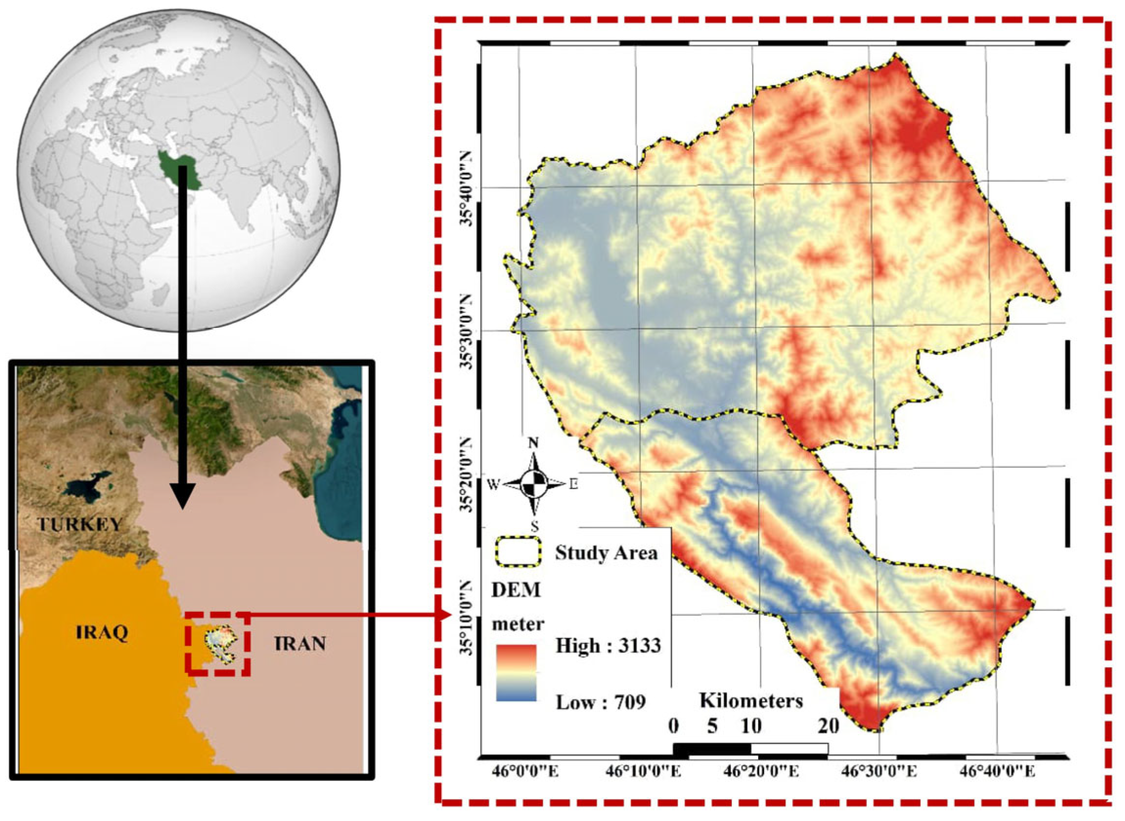
2.1. Study Area
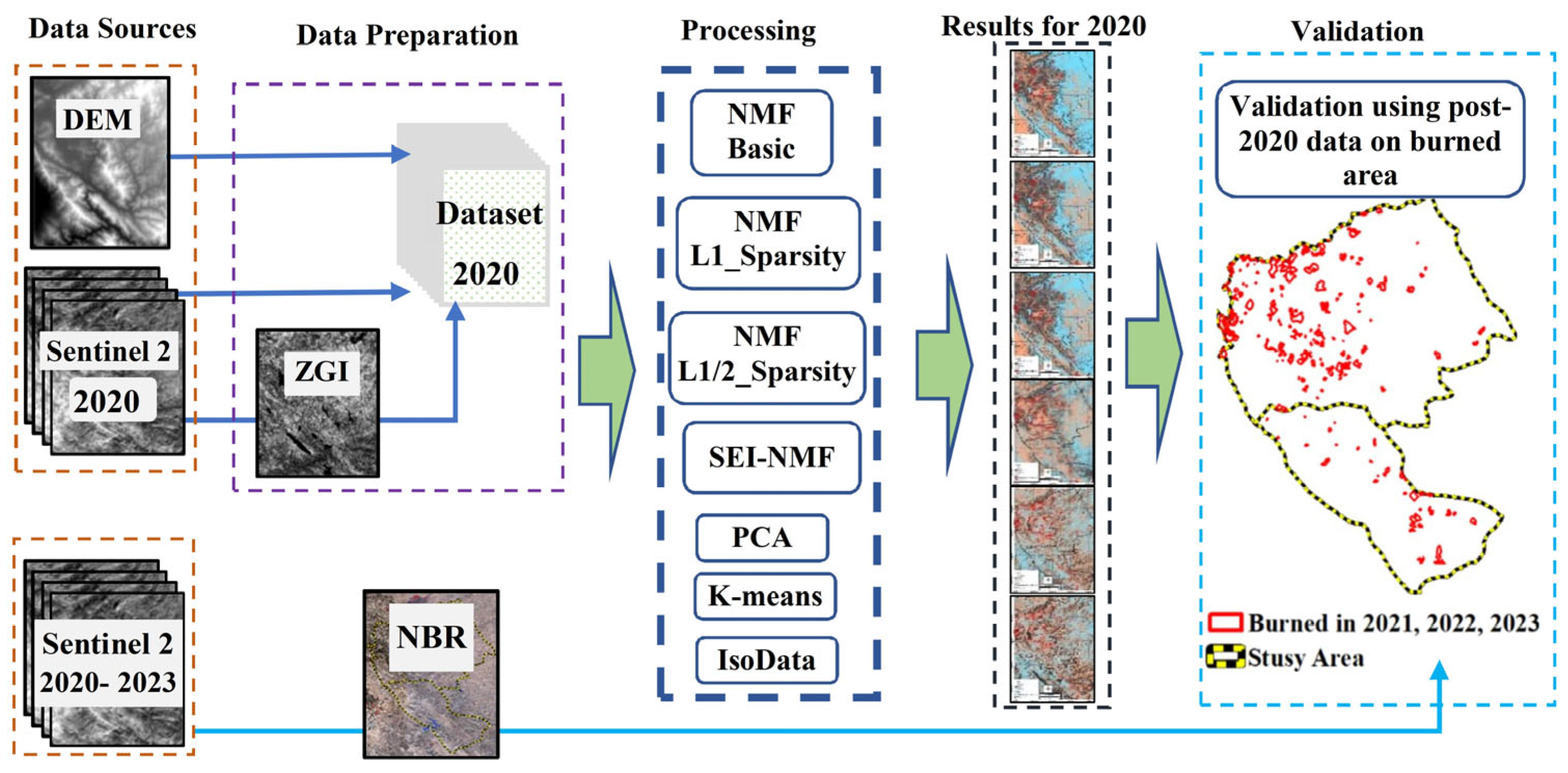
2.2. Data Sources
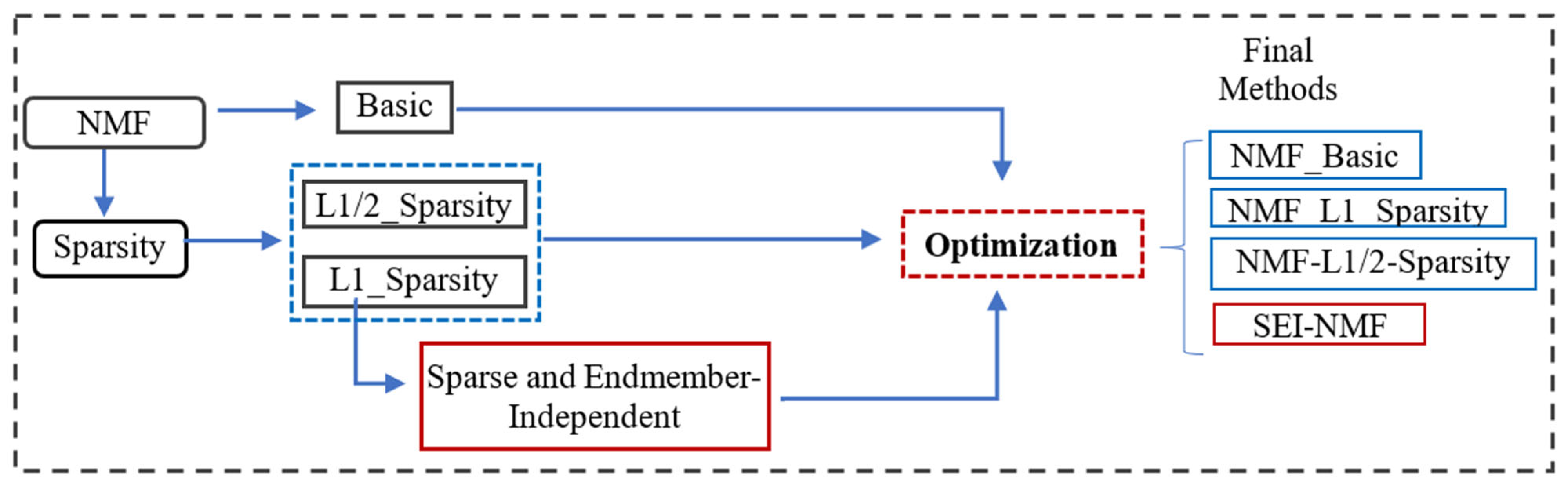
2.3. Sparse and Endmember-Independent Non-Negative Matrix Factorization (SEI-NMF)
2.3.1. Linear Mixture Model (LMM)
2.3.2. Non-Negative Matrix Factorization (NMF_Basic)
2.3.3. Sparsity Regularizer (NMF_L1- and L1/2-Sparsity)
2.3.4. Proposed Method (SEI-NMF)
2.3.5. Optimization
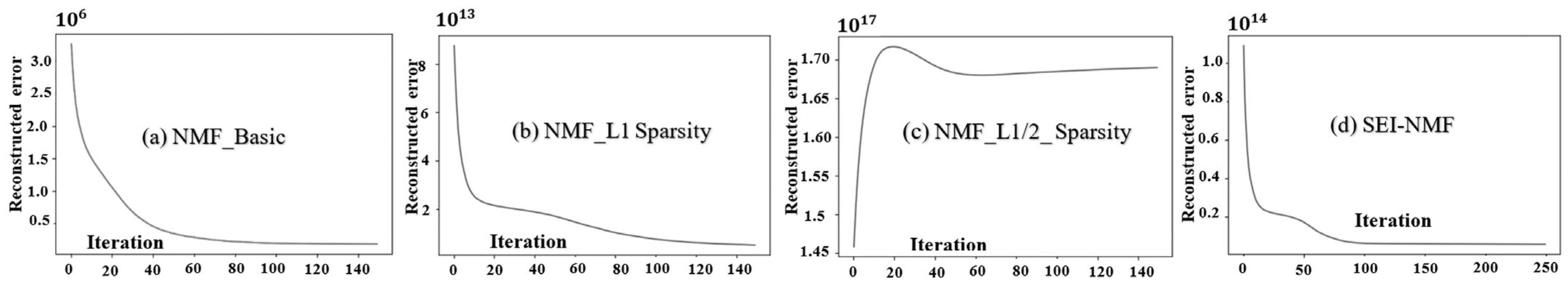
2.4. The Number of Components (Endmembers) and Iteration
2.5. Labelling and Validation
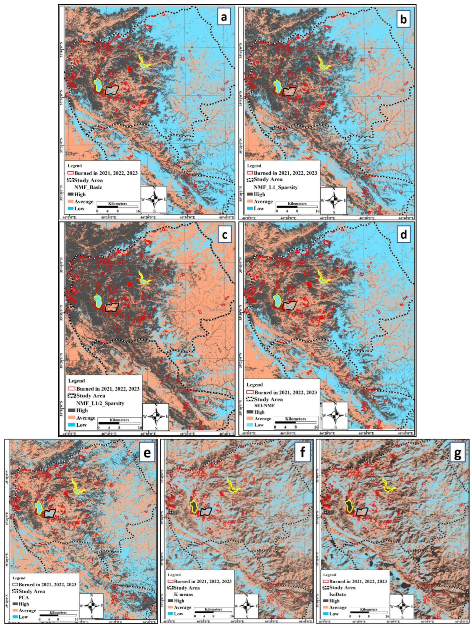
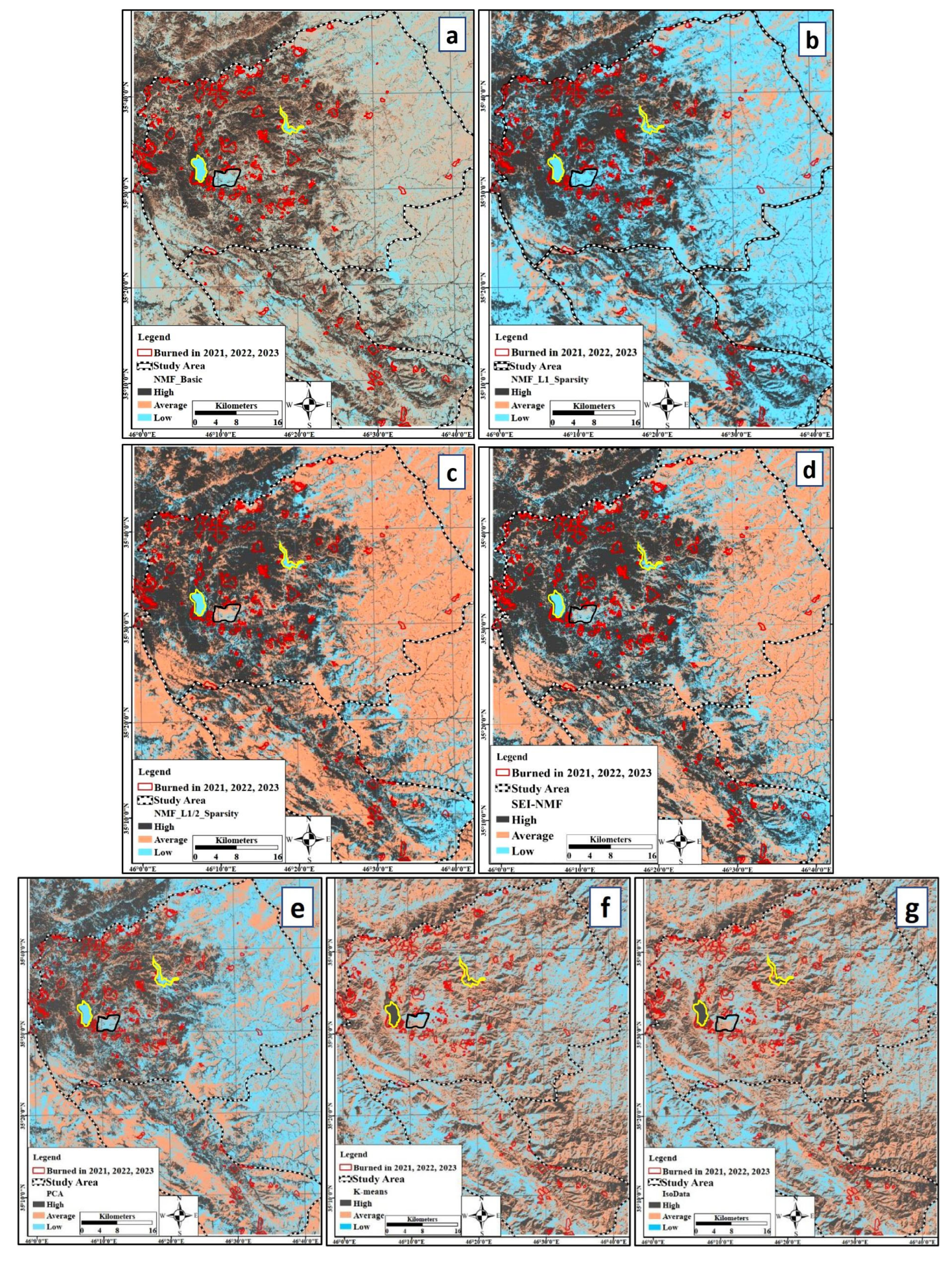
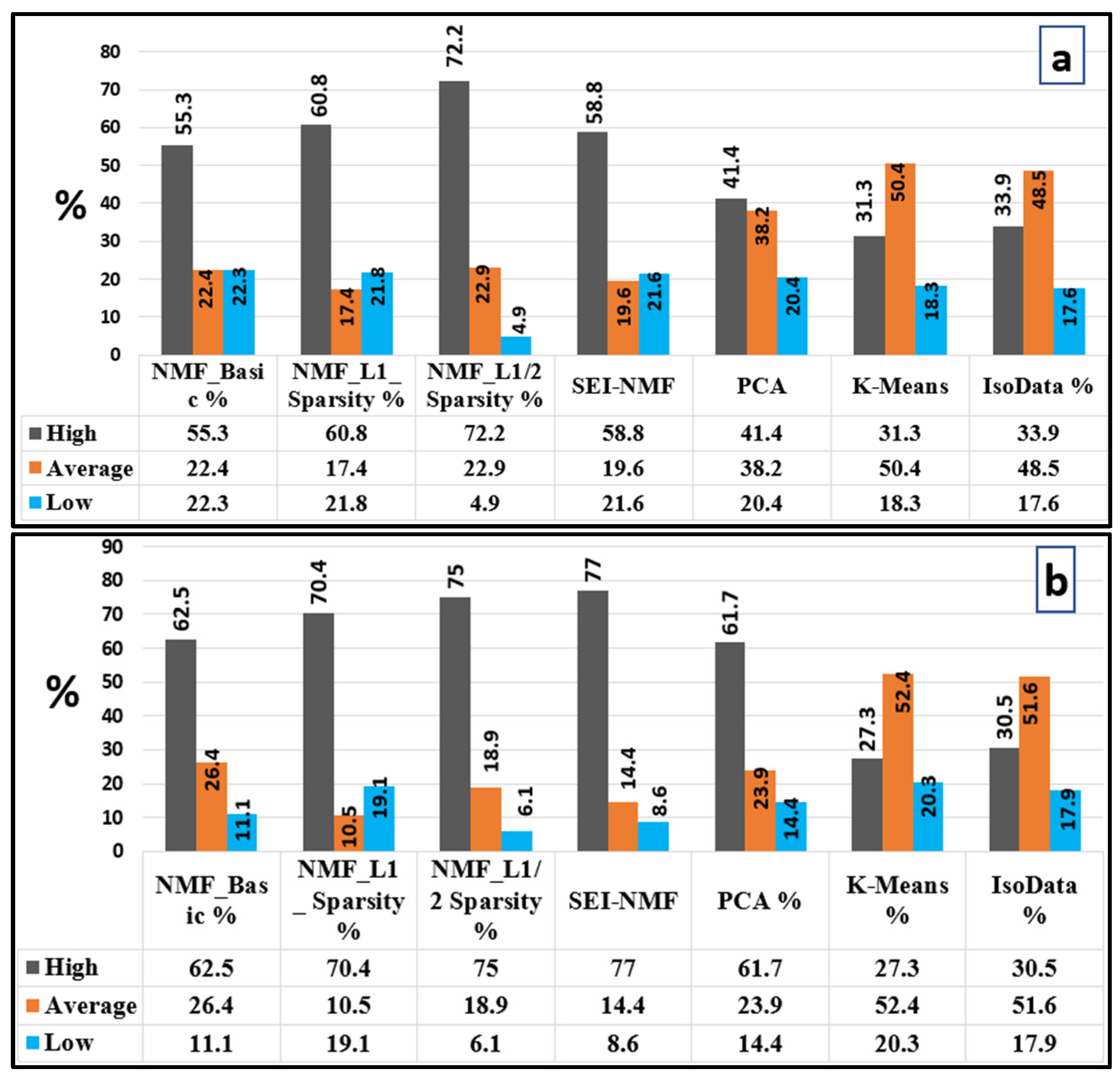
3. Results
4. Discussion
5. Conclusions
Author Contributions
Funding
Institutional Review Board Statement
Informed Consent Statement
Data Availability Statement
Acknowledgments
Conflicts of Interest
References
- Zema, D.A.; Nunes, J.P.; Lucas-Borja, M.E. Improvement of Seasonal Runoff and Soil Loss Predictions by the MMF (Morgan-Morgan-Finney) Model after Wildfire and Soil Treatment in Mediterranean Forest Ecosystems. Catena 2020, 188, 104415. [Google Scholar] [CrossRef]
- Bowman, D.M.J.S.; Moreira-Muñoz, A.; Kolden, C.A.; Chavez, R.O.; Munoz, A.A.; Salinas, F.; Gonzalez-Reyes, A.; Rocco, R.; de la Barrera, F.; Williamson, G.J.; et al. Human-environmental drivers and impacts of the globally extreme 2017 Chilean fires. Ambio 2019, 48, 350–362. [Google Scholar] [CrossRef]
- Geist, H.J.; Lambin, E.F. Proximate Causes and Underlying Driving Forces of Tropical Deforestation. BioScience 2002, 52, 143–150. [Google Scholar] [CrossRef]
- Suryabhagavan, K.V.; Alemu, M.; Balakrishnan, M. GIS-Based Multi-Criteria Decision Analysis for Forest Fire Susceptibility Mapping: A Case Study in Harenna Forest, Southwestern Ethiopia. Trop. Ecol. 2016, 57, 33–43. [Google Scholar]
- Dos Reis, M.; Graça, P.M.L.d.A.; Yanai, A.M.; Ramos, C.J.P.; Fearnside, P.M. Forest Fires and Deforestation in the Central Amazon: Effects of Landscape and Climate on Spatial and Temporal Dynamics. J. Environ. Manag. 2021, 288, 112310. [Google Scholar] [CrossRef]
- Kala, C.P. Environmental and socioeconomic impacts of forest fires: A call for multilateral cooperation and management interventions. Nat. Hazards Res. 2023, 3, 286–294. [Google Scholar] [CrossRef]
- Keenan, R.J. Climate Change Impacts and Adaptation in Forest Management: A Review. Ann. For. Sci. 2015, 72, 145–167. [Google Scholar] [CrossRef]
- Simioni, G.; Marie, G.; Davi, H.; Martin-St Paul, N.; Huc, R. Natural Forest Dynamics Have More Influence than Climate Change on the Net Ecosystem Production of a Mixed Mediterranean Forest. Ecol. Model. 2020, 416, 108921. [Google Scholar] [CrossRef]
- Rahimi, I.; Duarte, L.; Teodoro, A.C. Zagros Grass Index—A New Vegetation Index to Enhance Fire Fuel Mapping: A Case Study in the Zagros Mountains. Sustainability 2024, 16, 3900. [Google Scholar] [CrossRef]
- Teodoro, A.C.; Duarte, L. Forest fire risk maps: A GIS open source application—A case study in Norwest of Portugal. Int. J. Geogr. Inf. Sci. 2013, 27, 699–720. [Google Scholar] [CrossRef]
- Ghorbanzadeh, O.; Valizadeh, K.K.; Blaschke, T.; Aryal, J.; Naboureh, A.; Einali, J.; Bian, J. Spatial Prediction of Wildfire Susceptibility Using Field Survey GPS Data and Machine Learning Approaches. Fire 2019, 2, 43. [Google Scholar] [CrossRef]
- Gong, J.; Jin, T.; Cao, E.; Wang, S.; Yan, L. Is Ecological Vulnerability Assessment Based on the VSD Model and AHP-Entropy Method Useful for Loessial Forest Landscape Protection and Adaptive Management? A Case Study of Ziwuling Mountain Region, China. Ecol. Indic. 2022, 143, 109379. [Google Scholar] [CrossRef]
- Lamat, R.; Kumar, M.; Kundu, A.; Lal, D. Forest Fire Risk Mapping Using Analytical Hierarchy Process (AHP) and Earth Observation Datasets: A Case Study in the Mountainous Terrain of Northeast India. SN Appl. Sci. 2021, 3, 425. [Google Scholar] [CrossRef]
- Arca, D.; Hacısalihoğlu, M.; Kutoğlu, Ş.H. Producing Forest Fire Susceptibility Map via Multi-Criteria Decision Analysis and Frequency Ratio Methods. Nat. Hazards 2020, 104, 73–89. [Google Scholar] [CrossRef]
- Tiwari, A.; Shoab, M.; Dixit, A. GIS-Based FFS Modeling in Pauri Garhwal, India: A Comparative Assessment of Frequency Ratio, Analytic Hierarchy Process, and Fuzzy Modeling Techniques. Nat. Hazards 2021, 105, 1189–1230. [Google Scholar] [CrossRef]
- Moayedi, H.; Mehrabi, M.; Bui, D.T.; Pradhan, B.; Foong, L.K. Fuzzy-Metaheuristic Ensembles for Spatial Assessment of Forest Fire Susceptibility. J. Environ. Manag. 2020, 260, 109867. [Google Scholar] [CrossRef]
- Shi, C.; Zhang, F. A forest fire susceptibility modeling approach based on integration of machine learning algorithms. Forests 2023, 14, 1506. [Google Scholar] [CrossRef]
- Trucchia, A.; Meschi, G.; Fiorucci, P.; Gollini, A.; Negro, D. Defining wildfire susceptibility maps in Italy for understanding seasonal wildfire regimes at the national level. Fire 2022, 5, 30. [Google Scholar] [CrossRef]
- Saha, S.; Bera, B.; Shit, P.K.; Bhattacharjee, S.; Sengupta, N. Prediction of forest fire susceptibility applying machine and deep learning algorithms for conservation priorities of forest resources. Remote Sens. Appl. Soc. Environ. 2023, 29, 100917. [Google Scholar] [CrossRef]
- Piao, Y.; Lee, D.; Park, S.; Kim, H.G.; Jin, Y. Forest fire susceptibility assessment using Google Earth Engine in Gangwon-do, Republic of Korea. Geomat. Nat. Hazards Risk 2022, 13, 432–450. [Google Scholar] [CrossRef]
- Kalantar, B.; Ueda, N.; Idrees, M.O.; Janizadeh, S.; Ahmadi, K.; Shabani, F. Forest fire susceptibility prediction based on machine learning models with resampling algorithms on remote sensing data. Remote Sens. 2020, 12, 3682. [Google Scholar] [CrossRef]
- Mishra, M.; Guria, R.; Baraj, B.; Nanda, A.P.; Santos, C.A.G.; Da Silva, R.M.; Laksono, F.A.T. Spatial analysis and machine learning prediction of forest fire susceptibility: A comprehensive approach for effective management and mitigation. Sci. Total Environ. 2024, 926, 171713. [Google Scholar] [CrossRef] [PubMed]
- Sharma, L.K.; Gupta, R.; Naureen Fatima, N. Assessing the predictive efficacy of six machine learning algorithms for the susceptibility of Indian forests to fire. Int. J. Wildland Fire 2022, 31, 735–758. [Google Scholar] [CrossRef]
- Maffei, C.; Menenti, M. An application of the perpendicular moisture index for the prediction of fire hazard. EARSel eProceedings 2014, 13, 13–19. [Google Scholar]
- Sulova, A.; Arsanjani, J.J. Exploratory Analysis of Driving Force of Wildfires in Australia: An Application of Machine Learning within Google Earth Engine. Remote Sens. 2020, 13, 10. [Google Scholar] [CrossRef]
- Sivrikaya, F.; Küçük, Ö. Modeling forest fire risk based on GIS-based analytical hierarchy process and statistical analysis in the Mediterranean region. Ecol. Inform. 2021, 68, 101537. [Google Scholar] [CrossRef]
- Chaleplis, K.; Walters, A.; Fang, B.; Lakshmi, V.; Gemitzi, A. A Soil Moisture and Vegetation-Based Susceptibility Mapping approach to wildfire events in Greece. Remote Sens. 2024, 16, 1816. [Google Scholar] [CrossRef]
- Chuvieco, E.; Cocero, D.; Riaño, D.; Martin, P.; Martínez-Vega, J.; De La Riva, J.; Pérez, F. Combining NDVI and surface temperature for the estimation of live fuel moisture content in forest fire danger rating. Remote Sens. Environ. 2004, 92, 322–331. [Google Scholar] [CrossRef]
- Luz, A.E.O.; Negri, R.G.; Massi, K.G.; Colnago, M.; Silva, E.A.; Casaca, W. Mapping fire susceptibility in the Brazilian Amazon forests using multitemporal remote sensing and time-varying unsupervised anomaly detection. Remote Sens. 2022, 14, 2429. [Google Scholar] [CrossRef]
- Yankovich, K.S.; Yankovich, E.P.; Baranovskiy, N.V. Classification of vegetation to estimate forest fire danger using LANDSAT 8 Images: Case study. Math. Probl. Eng. 2019, 2019, 6296417. [Google Scholar] [CrossRef]
- Zaidi, A. Predicting wildfires in Algerian forests using machine learning models. Heliyon 2023, 9, e18064. [Google Scholar] [CrossRef] [PubMed]
- Wang, M.; Gao, G.; Huang, H.; Heidari, A.A.; Zhang, Q.; Chen, H.; Tang, W. A principal component Analysis-Boosted dynamic Gaussian mixture clustering model for ignition factors of Brazil’s rainforests. IEEE Access 2021, 9, 145748–145762. [Google Scholar] [CrossRef]
- Thein, A.M.; Htwe, A.N. Based on Principal Component Analysis of Land Use Land Cover Change Detection Using Landsat Satellite Images (Case Study Mandalay City). In Proceedings of the 2023 IEEE Conference on Computer Applications (ICCA), Yangon, Myanmar, 27–28 February 2023; pp. 147–152. [Google Scholar] [CrossRef]
- Sadeghi, V.; Ebadi, H.; Sadeghi, V.; Moghimi, A. Automatic Land Use/Land Cover Change Detection from Multitemporal Remote Sensed Images and Old Maps by Refining of Training Data Based on Chi-Square Test and K-Means Clustering. J. Geomatics Sci. Technol. 2021, 10, 143–161. Available online: http://jgst.issgeac.ir/article-1-935-en.html (accessed on 10 April 2025).
- Jarocińska, A.; Kopeć, D.; Kycko, M. Comparison of Dimensionality Reduction Methods on Hyperspectral Images for the Identification of Heathlands and Mires. Sci. Rep. 2024, 14, 27662. [Google Scholar] [CrossRef] [PubMed]
- Ma, Z.; Liu, Z.; Zhao, Y.; Zhang, L.; Liu, D.; Ren, T.; Zhang, X.; Li, S. An Unsupervised Crop Classification Method Based on Principal Components Isometric Binning. ISPRS Int. J. Geo-Inf. 2020, 9, 648. [Google Scholar] [CrossRef]
- Lv, Z.; Liu, T.; Shi, C.; Benediktsson, J.A.; Du, H. Novel Land Cover Change Detection Method Based on K-Means Clustering and Adaptive Majority Voting Using Bitemporal Remote Sensing Images. IEEE Access 2019, 7, 34425–34437. [Google Scholar] [CrossRef]
- Lillesand, T.; Kiefer, R. Remote Sensing and Image Interpretation, 4th ed.; Wiley: New York, NY, USA, 2000. [Google Scholar]
- Bioucas-Dias, J.M.; Plaza, A.; Dobigeon, N.; Parente, M.; Du, Q.; Gader, P.; Chanussot, J. Hyperspectral Unmixing Overview: Geometrical, Statistical, and Sparse Regression-Based Approaches. IEEE J. Sel. Top. Appl. Earth Obs. Remote Sens. 2012, 5, 354–379. [Google Scholar] [CrossRef]
- Huang, R.; Jiao, H.; Li, X.; Chen, S.; Xia, C. Hyperspectral unmixing using robust deep nonnegative matrix factorization. Remote Sens. 2023, 15, 2900. [Google Scholar] [CrossRef]
- Settembre, G.; Taggio, N.; Del Buono, N.; Esposito, F.; Di Lauro, P.; Aiello, A. A land cover change framework analyzing wildfire-affected areas in bitemporal PRISMA hyperspectral images. Math. Comput. Simul. 2024, 229, 855–866. [Google Scholar] [CrossRef]
- Berry, M.W.; Browne, M.; Langville, A.N.; Pauca, V.P.; Plemmons, R.J. Algorithms and Applications for Approximate Nonnegative Matrix Factorization. Comput. Stat. Data Anal. 2007, 52, 155–173. [Google Scholar] [CrossRef]
- Gillis, N.; Kuang, D.; Park, H. Hierarchical clustering of hyperspectral images using Rank-Two nonnegative matrix factorization. IEEE Trans. Geosci. Remote Sens. 2014, 53, 2066–2078. [Google Scholar] [CrossRef]
- Van Nguyen, L.; Lee, G. Underutilized Feature Extraction Methods for Burn Severity Mapping: A Comprehensive Evaluation. Remote Sens. 2024, 16, 4339. [Google Scholar] [CrossRef]
- Harries, D.; O’Kane, T.J. Applications of matrix factorization methods to climate data. Nonlinear Process. Geophys. 2020, 27, 453–471. [Google Scholar] [CrossRef]
- Zhu, X.; Li, M.; Deng, Y.; Luo, X.; Shen, L.; Long, C. L2,1-Norm Regularized Double Non-Negative Matrix Factorization for Hyperspectral Change Detection. Symmetry 2025, 17, 304. [Google Scholar] [CrossRef]
- Guillaume, M.; Minghelli, A.; Deville, Y.; Chami, M.; Juste, L.; Lenot, X.; Lafrance, B.; Jay, S.; Briottet, X.; Serfaty, V. Mapping Benthic Habitats by Extending Non-Negative Matrix Factorization to Address the Water Column and Seabed Adjacency Effects. Remote Sens. 2020, 12, 2072. [Google Scholar] [CrossRef]
- Esi, Ç.; Ertürk, A.; Erten, E. Nonnegative matrix factorization-based environmental monitoring of marine mucilage. Int. J. Remote Sens. 2024, 45, 3764–3788. [Google Scholar] [CrossRef]
- Yokoya, N.; Chan, J.C.-W.; Segl, K. Potential of resolution-enhanced hyperspectral data for mineral mapping using simulated EnMAP and Sentinel-2 images. Remote Sens. 2016, 8, 172. [Google Scholar] [CrossRef]
- Khader, A.; Yang, J.; Xiao, L. NMF-DUNET: Nonnegative matrix factorization inspired deep unrolling networks for hyperspectral and multispectral image fusion. IEEE J. Sel. Top. Appl. Earth Obs. Remote Sens. 2022, 15, 5704–5720. [Google Scholar] [CrossRef]
- Hou, W.; Liu, X.; Wang, J.; Chen, C.; Xu, X. Multispectral Land Surface Reflectance Reconstruction Based on Non-Negative Matrix Factorization: Bridging Spectral Resolution Gaps for GRASP TROPOMI BRDF Product in Visible. Remote Sens. 2025, 17, 1053. [Google Scholar] [CrossRef]
- Mupfiga, U.N.; Mutanga, O.; Dube, T.; Kowe, P. Spatial Clustering of Vegetation Fire Intensity Using MODIS Satellite Data. Atmosphere 2022, 13, 1972. [Google Scholar] [CrossRef]
- Elhag, M.; Yilmaz, N.; Bahrawi, J.; Al-Ghamdi, K.; Mansour, K. Evaluation of Optical Remote Sensing Data in Burned Areas Mapping of Thasos Island, Greece. Earth Syst. Environ. 2020, 4, 813–826. [Google Scholar] [CrossRef]
- Jazirehi, M.H.; Rostaaghi, E.M. Silviculture in Zagros; University of Tehran Press: Tehran, Iran, 2003; 560p, Available online: https://www.scirp.org/reference/referencespapers?referenceid=1852053 (accessed on 20 November 2023).
- El-Moslimany, A.P. Ecology and Late-Quaternary History of the Kurdo-Zagrosian Oak Forest Near Lake Zeribar, Western Iran. Vegetation 1986, 68, 55–63. [Google Scholar] [CrossRef]
- Google Earth Engine Team. COPERNICUS/S2: Sentinel-2 MSI: MultiSpectral Instrument, Level-1C; Google Earth Engine: 2025. Available online: https://developers.google.com/earth-engine/datasets/catalog/COPERNICUS_S2 (accessed on 20 February 2025).
- USGS EROS Archive. Digital Elevation—Shuttle Radar Topography Mission (SRTM). Available online: https://www.usgs.gov/centers/eros/science/usgs-eros-archive-digital-elevation-shuttle-radar-topography-mission-srtm-1 (accessed on 22 February 2025).
- National Cartographic Center of Iran. Administrative Boundaries Vector Data. Available online: https://www.ncc.gov.ir (accessed on 20 February 2025).
- Qian, Y.; Jia, S.; Zhou, J.; Robles-Kelly, A. Hyperspectral unmixing via L1/2 sparsity-constrained nonnegative matrix factorization. IEEE Trans. Geosci. Remote Sens. 2011, 49, 4282–4297. [Google Scholar] [CrossRef]
- Huang, Q.; Yin, X.; Chen, S.; Wang, Y.; Chen, B. Robust Nonnegative Matrix Factorization with Structure Regularization. Neurocomputing 2020, 412, 72–90. [Google Scholar] [CrossRef]
- Faraji, M.; Seyedi, S.A.; Akhlaghian Tab, F.; Mahmoodi, R. Multi-label feature selection with global and local label correlation. Expert Syst. With Appl. 2024, 246, 123198. [Google Scholar] [CrossRef]
- Li, H.; Li, K.; An, J.; Zhang, W.; Li, K. An efficient manifold regularized sparse non-negative matrix factorization model for large-scale recommender systems on GPUs. Inf. Sci. 2019, 496, 464–484. [Google Scholar] [CrossRef]
- Liu, X.; Wang, W.; He, D.; Jiao, P.; Jin, D.; Cannistraci, C.V. Semi-supervised community detection based on non-negative matrix factorization with node popularity. Inf. Sci. 2017, 381, 304–321. [Google Scholar] [CrossRef]
- Seyedi, S.A.; Tab, F.A.; Lotfi, A.; Salahian, N.; Chavoshinejad, J. Elastic adversarial deep nonnegative matrix factorization for matrix completion. Inf. Sci. 2023, 621, 562–579. [Google Scholar] [CrossRef]
- Lee, D.D.; Seung, H.S. Algorithms for non-negative matrix factorization. In Proceedings of the 2000 Conference on Advances in Neural Information Processing Systems, Denver, CO, USA, 1 January 2000; MIT Press: Cambridge, MA, USA, 2001; pp. 556–562. [Google Scholar]
- Lu, X.; Wu, H.; Yuan, Y.; Yan, P.; Li, X. Manifold regularized sparse NMF for hyperspectral unmixing. IEEE Trans. Geosci. Remote Sens. 2013, 51, 2815–2826. [Google Scholar] [CrossRef]
- Xu, R.; Wunsch, D. Survey of clustering algorithms. IEEE Trans. Neural Netw. 2005, 16, 645–678. [Google Scholar] [CrossRef]
- Kang, J.; Wang, Z.; Sui, L.; Yang, X.; Ma, Y.; Wang, J. Consistency Analysis of Remote Sensing Land Cover Products in the Tropical Rainforest Climate Region: A Case Study of Indonesia. Remote Sens. 2020, 12, 1410. [Google Scholar] [CrossRef]
- Wei, R.; Ye, C.; Sui, T.; Ge, Y.; Li, Y.; Li, J. Combining Spatial Response Features and Machine Learning Classifiers for Landslide Susceptibility Mapping. Int. J. Appl. Earth Obs. Geoinf. 2022, 107, 102681. [Google Scholar] [CrossRef]
- Meyer, H.; Pebesma, E. Machine Learning-Based Global Maps of Ecological Variables and the Challenge of Assessing Them. Nat. Commun. 2022, 13, 29838. [Google Scholar] [CrossRef]
- Giddey, B.L.; Baard, J.A.; Kraaij, T. Verification of the differenced Normalised Burn Ratio (dNBR) as an index of fire severity in Afrotemperate Forest. S. Afr. J. Bot. 2021, 146, 348–353. [Google Scholar] [CrossRef]
- Sivrikaya, F.; Günlü, A.; Küçük, Ö.; Ürker, O. Forest fire risk mapping with Landsat 8 OLI images: Evaluation of the potential use of vegetation indices. Ecol. Inform. 2024, 79, 102461. [Google Scholar] [CrossRef]
- Guo, Z.; Min, A.; Yang, B.; Chen, J.; Li, H. A Modified Huber Nonnegative Matrix Factorization Algorithm for Hyperspectral Unmixing. IEEE J. Sel. Top. Appl. Earth Obs. Remote Sens. 2021, 14, 5559–5571. [Google Scholar] [CrossRef]
- Bari, M.H.; Ahmed, T.; Afjal, M.I.; Nitu, A.M.; Uddin, M.P.; Marjan, M.A. Segmented Nonnegative Matrix Factorization for Hyperspectral Image Classification. In Proceedings of the International Conference on Electrical, Computer and Communication Engineering (ECCE), Chittagong, Bangladesh, 23–25 February 2023; pp. 1–5. [Google Scholar] [CrossRef]
- Zhao, L.; Zhuang, G.; Xu, X. Facial expression recognition based on PCA and NMF. In Proceedings of the 7th World Congress on Intelligent Control and Automation (WCICA), Chongqing, China, 25–27 June 2008; pp. 6826–6829. [Google Scholar] [CrossRef]
- Zheng, Z.; Zeng, Y.; Zou, B.; Xie, Q.; Xian, W.; Xu, W.; Liu, Y.; Liu, Z. Assessing the burn severity of wildfires by incorporating vegetation structure information. Geomat. Nat. Hazards Risk 2024, 15, 1. [Google Scholar] [CrossRef]
- Henry, M.C. Comparison of single- and multi-date Landsat data for mapping wildfire scars in Ocala National Forest, Florida. Photogramm. Eng. Remote Sens. 2008, 74, 881–891. [Google Scholar] [CrossRef]
- Epting, J.; Verbyla, D.; Sorbel, B. Evaluation of remotely sensed indices for assessing burn severity in interior Alaska using Landsat TM and ETM+. Remote Sens. Environ. 2005, 96, 328–339. [Google Scholar] [CrossRef]
- Oladimeji, M.O.; Ghavami, M.; Dudley, S. A new approach for event detection using k-means clustering and neural networks. In Proceedings of the International Joint Conference on Neural Networks (IJCNN), Killarney, Ireland, 12–17 July 2015. [Google Scholar] [CrossRef]
- Lakshmanaswamy, P.; Sundaram, A.; Sudanthiran, T. Prioritizing the right to environment: Enhancing forest fire detection and prevention through satellite data and machine learning algorithms for early warning systems. Remote Sens. Earth Syst. Sci. 2024, 7, 472–485. [Google Scholar] [CrossRef]

| Data Type | Projection System | Spatial Resolution (m) | Time Period | Source |
|---|---|---|---|---|
| Sentinel-2 | UTM | 10 | 2020–2023 | [56] |
| DEM SRTM | UTM | 10 | 2000 | [57] |
| Vector data: study area, water body, town border | UTM | - | - | [58] |
| First Scenario (%) | Second Scenario (%) | |||||||
|---|---|---|---|---|---|---|---|---|
| Method | TP | FP | FN | TN | TP | FP | FN | TN |
| NMF-Basic | 1.95 | 28.32 | 1.57 | 68.16 | 2.2 | 33.19 | 1.32 | 63.3 |
| NMF-L1 | 2.14 | 31.74 | 1.38 | 64.74 | 2.48 | 37.09 | 1.04 | 59.4 |
| NMF-L1/2 | 2.54 | 41.77 | 0.98 | 54.71 | 2.64 | 38.88 | 0.88 | 57.61 |
| SEI-NMF | 2.07 | 28.52 | 1.45 | 67.96 | 2.71 | 38.58 | 0.81 | 57.9 |
| PCA | 1.46 | 26.48 | 2.06 | 70.01 | 2.17 | 30.56 | 1.35 | 65.93 |
| K-Means | 1.1 | 24.6 | 2.42 | 71.88 | 0.96 | 24.7 | 2.55 | 71.79 |
| IsoData | 1.19 | 27.06 | 2.33 | 69.42 | 1.08 | 27.08 | 2.44 | 69.4 |
| Method | Precision (%) | Recall (%) | F1-Score (%) | Specificity (%) | Balanced Acc. (%) | χ2 | p-Value |
|---|---|---|---|---|---|---|---|
| NMF-Basic | 6.43 | 55.30 | 11.52 | 70.65 | 62.97 | 354,027.69 | <0.0001 |
| NMF-L1 | 6.31 | 60.77 | 11.44 | 67.10 | 63.94 | 385,646.66 | <0.0001 |
| NMF-L1/2 | 5.73 | 72.18 | 10.62 | 56.71 | 64.45 | 375,753.54 | <0.0001 |
| SEI-NMF | 6.76 | 58.78 | 12.13 | 70.44 | 64.61 | 446,861.95 | <0.0001 |
| PCA | 5.21 | 41.36 | 9.26 | 72.56 | 56.96 | 107,401.38 | <0.0001 |
| K-Means | 4.27 | 31.29 | 7.21 | 74.57 | 52.93 | 228,209.04 | <0.0001 |
| IsoData | 4.22 | 33.88 | 7.39 | 71.94 | 52.91 | 212,653.11 | <0.0001 |
| Method | Precision (%) | Recall (%) | F1-Score (%) | Specificity (%) | Balanced Acc. (%) | χ2 | p-Value |
|---|---|---|---|---|---|---|---|
| NMF-Basic | 6.21 | 62.51 | 11.3 | 65.6 | 64.06 | 383,639 | <0.0001 |
| NMF-L1 | 6.27 | 70.5 | 11.51 | 61.56 | 66.03 | 477,239 | <0.0001 |
| NMF-L1/2 | 6.36 | 75 | 11.72 | 59.71 | 67.35 | 550,592 | <0.0001 |
| SEI-NMF | 6.56 | 77 | 12.09 | 60.01 | 68.51 | 627,079 | <0.0001 |
| PCA | 6.63 | 61.68 | 11.97 | 68.33 | 65.01 | 454,071 | <0.0001 |
| K-Means | 3.75 | 27.38 | 6.6 | 74.4 | 50.89 | 1844.85 | <0.0001 |
| IsoData | 3.82 | 30.59 | 6.11 | 71.94 | 51.26 | 3494.24 | <0.0001 |
Disclaimer/Publisher’s Note: The statements, opinions and data contained in all publications are solely those of the individual author(s) and contributor(s) and not of MDPI and/or the editor(s). MDPI and/or the editor(s) disclaim responsibility for any injury to people or property resulting from any ideas, methods, instructions or products referred to in the content. |
© 2025 by the authors. Licensee MDPI, Basel, Switzerland. This article is an open access article distributed under the terms and conditions of the Creative Commons Attribution (CC BY) license (https://creativecommons.org/licenses/by/4.0/).
Share and Cite
Rahimi, I.; Duarte, L.; Barkhoda, W.; Teodoro, A.C. Comparative Analysis of Non-Negative Matrix Factorization in Fire Susceptibility Mapping: A Case Study of Semi-Mediterranean and Semi-Arid Regions. Land 2025, 14, 1334. https://doi.org/10.3390/land14071334
Rahimi I, Duarte L, Barkhoda W, Teodoro AC. Comparative Analysis of Non-Negative Matrix Factorization in Fire Susceptibility Mapping: A Case Study of Semi-Mediterranean and Semi-Arid Regions. Land. 2025; 14(7):1334. https://doi.org/10.3390/land14071334
Chicago/Turabian StyleRahimi, Iraj, Lia Duarte, Wafa Barkhoda, and Ana Cláudia Teodoro. 2025. "Comparative Analysis of Non-Negative Matrix Factorization in Fire Susceptibility Mapping: A Case Study of Semi-Mediterranean and Semi-Arid Regions" Land 14, no. 7: 1334. https://doi.org/10.3390/land14071334
APA StyleRahimi, I., Duarte, L., Barkhoda, W., & Teodoro, A. C. (2025). Comparative Analysis of Non-Negative Matrix Factorization in Fire Susceptibility Mapping: A Case Study of Semi-Mediterranean and Semi-Arid Regions. Land, 14(7), 1334. https://doi.org/10.3390/land14071334