Trade-Offs and Synergies of Ecosystem Services in Terminal Lake Basins of Arid Regions Under Environmental Change: A Case Study of the Ebinur Lake Basin

Abstract

As essential components of arid region ecosystems, terminal lakes play a critical role in enhancing the functions of ecosystem services (ESs) and improving ecological structure. Despite the increasing degradation of ESs and landscape stability due to climate and human pressures, comprehensive assessments of water provision, carbon storage, soil conservation, and habitat integrity in arid terminal lake regions are still lacking. Focusing on the Ebinur Lake Basin (ELB), this study employed the InVEST model to quantify ES changes from 2000 to 2020, combined with univariate regression, Pearson, and Spearman correlation analyses to explore their dynamic evolution. Landscape pattern indices calculated via Fragstats 4.2 further revealed trends in fragmentation, boundary complexity, and diversity. Results show that most ESs exhibited synergistic relationships, particularly between carbon sequestration and habitat quality (r = 0.45), observed clear trade-offs, such as between water yield and carbon sequestration (r = −0.47), underscoring the complexity of ecosystem interactions. Enhanced ES functions were associated with increased patch number, density, and shape complexity, while landscape diversity fluctuated. NDVI growth improved ES performance and reduced fragmentation, though changes in landscape metrics were largely driven by climate variability and socio-economic pressures, exacerbating fragmentation and weakening ecological stability. Overall, understanding the trade-offs and synergies among ESs in the ELB is crucial for informing sustainable development strategies.

1. Introduction

ESs are the direct and indirect benefits that human societies derive from ecosystems, stemming from their structure and functioning. These services are commonly categorized into four types: provisioning, regulating, supporting, and cultural services [1]. They reflect the critical functions of ecosystems in maintaining natural processes and providing human well-being [2]. However, climate change and socio-economic development have severely affected the current and future supply of ESs [3]. As a result, ES functions have continued to decline, and challenges such as ecological fragility persist [4]. In response, the United Nations launched the Millennium Ecosystem Assessment (MA) in 2000 [5,6] and proposed the 17 Sustainable Development Goals (SDGs) in 2015 [7]. However, in ecosystem management and land use, different services often exhibit either mutually restrictive or reinforcing relationships, referred to as trade-offs and synergies [8]. With the intensification of global environmental change and human activities, the stability and sustainability of ESs have been declining [9]. Optimizing trade-offs and enhancing synergies among diverse ESs [10], particularly given their variability, uneven spatial distribution [11], and selective human use, requires quantitative analysis and assessment [12]. Such analysis helps uncover the intrinsic relationships among ESs [13] and provides a robust theoretical foundation for achieving the Sustainable Development Goals (SDGs), thereby promoting the efficient and sustainable use of ecosystems [14]. Given the intricate and complex interactions among ESs [15], various assessment models have emerged accordingly [16]. They include the InVEST model, ARIES model, and SoLVES model [17,18,19]. Among these models, the InVEST model is the most widely used in the assessments of ESs in the Central Valley of California, the Great Lakes region, the Three Gorges Reservoir area, the Loess Plateau, as well as in studies on the impacts of urbanization and agricultural expansion [20]. The InVEST model is built upon Geographic Information System (GIS) and remote sensing (RS) technologies [21], providing a solid data foundation and theoretical basis for the scientific formulation of land use planning and ecological compensation policies [22]. The InVEST model has been widely applied. It also provides a scientific basis for addressing challenges such as climate change, land use transformation, and ecological degradation [23], thereby promoting the integrated management of watershed ecological integrity and socio-economic sustainability. Sallustio et al. and Terrado et al. used the InVEST model to assess habitat quality in Italian nature reserves and watersheds under different conservation planning scenarios [24], Martínez-Harms et al. employed the InVEST model to assess carbon storage, water conservation, and agricultural product provisioning services across various watersheds in multiple countries, providing a basis for policy making [25,26].

Terminal lake basins in arid regions serve as key ecological security nodes along the Belt and Road Initiative [27]. They also represent typical cases of inland lake shrinkage and ecological degradation on a global scale [28]. The subunits within the basin are highly sensitive to changes in natural and anthropogenic factors and exhibit significant ES functions such as water conservation, soil retention, and local microclimate regulation [29]. However, under the combined influence of climate change and irrigated agriculture [30], terminal lakes in arid regions have experienced catastrophic shrinkage, with large areas of lakebeds drying up and becoming exposed on the surface [31]. The degradation of ecological functions and the decline in service capacity have caused severe damage to the surrounding environment. Moreover, under the influence of human activities, variations in topography, hydrology, and land use have led to significant spatial heterogeneity in the changes in ES functions within terminal lake basins [32]. Certain parts of the basin have managed to retain some ecological regulation functions due to effective water resource management measures, such as ecological projects involving artificial water diversion [33]. In contrast, other parts of the basin have experienced intensified ecological fragmentation due to overexploitation or the impacts of extreme climate events [34]. This has led to a sharp decline in habitat quality and other ESs, thereby disrupting the ecological balance of the basin [35]. At present, the assessment of trade-offs and synergies among ESs in terminal lake basins of arid regions remains inadequate [36]. It is urgent to build a multi-scale comprehensive assessment system with the help of advanced remote sensing technology and quantitative models to provide a scientific basis for decision making on ecological protection, resource management, and sustainable development in the ELB [37,38].

The ELB characterized by persistent drought, strong winds, salt dust, salinization, and sandstorms has led to a continuous reduction in lake area and exposed ecological shifts, accompanied by severe trade-offs and synergies among ESs [39]. To this end, this study analyzes the spatiotemporal variation characteristics and investigates the trade-offs and synergies of ESs in the ELB. Based on this, the objectives of this study are as follows: (1) to quantify the spatiotemporal variations in landscape patterns within the basin and reveal the trends of landscape fragmentation over the past 20 years; (2) to quantify the spatiotemporal variations in ESs in the ELB; (3) to elucidate the trade-offs and synergies among different ESs within the basin; and (4) to clarify the impacts of climate, vegetation, and socio-economic factors on landscape patterns and ESs. Through the above research, this study aims to provide a solid theoretical foundation and decision-making support for the scientific construction of the ecological barrier and the sustainable development of ESs in the ELB.

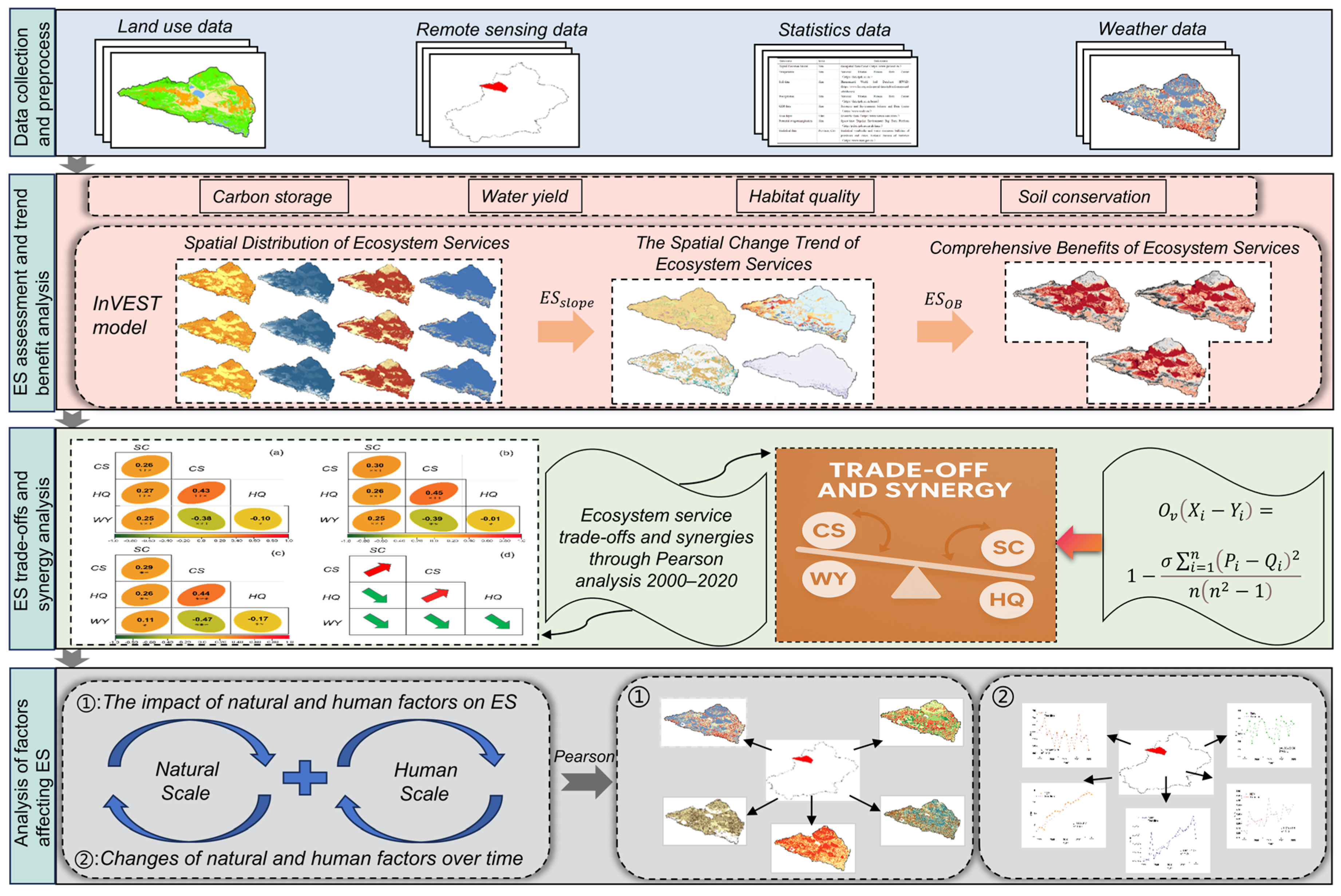
2. Materials and Methods

2.1. Study Area

The ELB (Figure 1) is situated deep within the interior of the Eurasian continent [40]. Located in the southwestern part of the Junggar Basin, the ELB is a typical terminal lake and serves as the main center for water and salt accumulation within the basin [41]. Due to its unique geographical location, with mountains on three sides blocking external airflows, the basin experiences an extreme climate characterized by scarce precipitation, abundant sunshine, high evaporation, and overall aridity. Water resources and ecosystems in the region are highly sensitive to climate change and significantly affected by its impacts [42]. The basin has a temperate continental climate with low precipitation and an average annual temperature of 5.6 °C [43]. In recent years, the annual average precipitation in the ELB has ranged between 116 and 170 mm, while the annual evaporation rate has exceeded 1000 mm, with evaporation far surpassing precipitation, demonstrating a distinctly arid characteristic [44]. The basin’s vegetation is primarily composed of grasslands, croplands, and bare land, with lakes occupying a relatively small area [45]. The diverse topography and various landscape types are intricately interwoven, jointly shaping the basin and providing a favorable foundation for in-depth analysis of the impacts of landscape patterns on ESs. In recent years, the rapid increase in population density (POP), continuous expansion of cultivated land, and sharp rise in per capita GDP have led to a dramatic surge in water demand, directly causing a significant shrinkage of Ebinur Lake’s surface area [46]. Large areas of natural vegetation have degraded and withered, desertification has intensified and spread, biodiversity has declined sharply, and the ecological security of the oasis is under serious threat [47]. The ecosystem and water resources of the ELB exhibit high vulnerability to land use change, making them highly susceptible to its adverse impacts and disturbances [48].

2.2. Data Sources

The data used in this study are mainly classified into three categories, with detailed information provided in

Table 1. Data sources and descriptions.

Data Name	Spatial Scale	Time Scale	Data Source
Digital Elevation Model	1 km	2000–2020	Geospatial Data Cloud (https://www.gscloud.cn/, accessed on 2 February 2025)
Land use type and NDVI	1 km	2000–2020	Resource and Environment Science and Data Center (https://www.resdc.cn/, accessed on 2 February 2025)
Temperature	1 km	2000–2020	National Tibetan Plateau Data Center (https://data.tpdc.ac.cn/, accessed on 8 February 2025)
Soil data	1 km	2000–2020	Harmonized World Soil Database (HWSD) (https://www.fao.org/soils-portal/data-hub/soil-maps-and-databases/, accessed on 8 February 2025)
Precipitation	1 km	2000–2020	National Tibetan Plateau Data Center (https://data.tpdc.ac.cn/home/, accessed on 8 February 2025)
GDP data	1 km	2000–2020	Resource and Environment Science and Data Center (https://www.resdc.cn/, accessed on 10 February 2025)

. The first category includes processed or semi-processed remote sensing data, including land use/land cover (LULC) types, Digital Elevation Model (DEM), Normalized Difference Vegetation Index (NDVI), and soil types. The second category includes observed data from meteorological stations, covering climatic factors such as potential evapotranspiration and precipitation. The third category comprises socio-economic data obtained from statistical yearbooks, mainly including indicators such as population and Gross Domestic Product (GDP). In this study, all spatial raster data were standardized to a 1 km resolution, covering the time period from 2000 to 2020.

2.3. Methods

2.3.1. Assessment of Landscape Pattern Changes

Fragstats software 4.2 is based on land LULC classification maps from different periods [49]. It calculates multiple landscape pattern indices at the patch level, class level, and landscape level to comprehensively assess the dynamic characteristics of spatial landscape patterns [50]. The key indices selected in this study include number of patches (NP), patch density (PD), The Landscape Shape Index (LSI), Shannon’s Diversity Index (SHDI), and Perimeter–Area Fractal Dimension (PAFRAC). These indices effectively reflect the degree of landscape fragmentation, spatial heterogeneity, and the distribution characteristics among different landscape types in the study area [51].

NP refers to the total number of discrete patches into which a specific land use type is divided within the landscape, and it is used to measure the degree of fragmentation of that landscape type [52]. This index helps assess the impact of human activities or natural disturbances on landscape patterns, and its variation is closely related to ES functions [53]. The specific formula is as follows:

$$NP=n$$

(1)

Here, NP represents the total number of patches in the landscape, where n is the actual number of patches. NP reflects the degree of landscape fragmentation.

Patch density refers to the NP per unit area and is used to measure the degree of landscape fragmentation [54]. As a key indicator for assessing landscape fragmentation, changes in patch density have a significant impact on ESs [55]. The specific formula is as follows:

Here, PD stands for patch density, representing the NP per unit area. N is the total NP, and A is the total area of the study region, usually expressed in hectares (ha) or square meters (m²).

$$PD={\displaystyle \raisebox{1ex}{$N$}\!\left/ \!\raisebox{-1ex}{$A$}\right.}$$

(2)

LSI is an indicator used to measure the complexity of landscape boundaries. It describes the irregularity and regularity of patch edges, reflecting the service capacity and sustainability of the ecosystem [56]. The complexity of landscape patches and the regularity of their boundaries depend on the value of LSI. The specific formula is as follows:

Here, LSI represents the Landscape Shape Index; E is the total boundary length of all patches within the landscape (typically in meters), and A is the total area of the study region (commonly in m² or ha). The units of A and E should be consistent—for example, if the area is in m², the boundary length should be in meters.

$$LSI={\displaystyle \frac{0.25E}{\sqrt{A}}}$$

(3)

PAFRAC is an important index in landscape ecology used to measure the complexity of patch shapes. It characterizes the geometric irregularity and fractal features of patch boundaries by analyzing the relationship between patch perimeter and area [57]. PAFRAC is closely associated with multiple ES functions, influencing ecological processes such as water yield, habitat quality, and carbon sequestration [58]. The specific formula is as follows:

$$PAFRAC={\displaystyle \frac{2\left[\left(n_i\sum _{j=1}^n\mathit{ln}{p}_{ij}^2\right)-{\left(\sum _{j=1}^n\mathit{ln}{p}_{ij}\right)}^2)\right]}{\left[n_j\sum _{j=1}^n\left(\mathit{ln}{p}_{ij}\times \mathit{ln}{a}_{ij}\right)\right]-\left[(\sum _{j=1}^n\mathit{ln}{p}_{ij}\times (\sum _{j=1}^n\mathit{ln}{a}_{ij})\right]}}$$

(4)

In the formula, PAFRAC stands for Perimeter–Area Fractal Dimension; n is the total NP; $p_{ij}$ is the perimeter of the j-th patch; and $a_{ij}$ is the area of the j-th patch. PAFRAC describes the fractal relationship between the perimeter and area of all patches within the landscape.

SHDI (Shannon’s Diversity Index) describes the richness (number of patch types) and evenness (proportional distribution of each type) of patches within the landscape. It is an important indicator for evaluating landscape diversity and a key metric for assessing the ES supply capacity and sustainability of the watershed [59]. The specific formula is as follows:

$$SHDI=-\sum _{i=1}^n{p}_i\mathit{ln}{p}_i$$

(5)

SHDI refers to Shannon’s Diversity Index; n is the total number of different landscape types (or species) in the landscape; and $p_i$ is the proportion of the i-th landscape type (or species).

2.3.2. Ecosystem Services Assessment

This study focuses on four representative ESs—carbon sequestration, water yield, soil retention, and habitat quality—reflecting key provisioning, regulating, and supporting functions in arid inland basins. These services are critical to regional ecological security, widely studied in terminal lake contexts, and well-suited for biophysical quantification using the InVEST model. Based on the InVEST model, this study conducted a multi-scale quantitative assessment of topical Ess, namely, carbon sequestration, water yield, soil retention, and habitat quality—in the ELB from 2000 to 2020 [60]. Carbon sequestration is a vital ES through which vegetation and soil absorb and store carbon dioxide, directly contributing to global climate regulation [61]. Its level reflects the ecosystem’s buffering capacity against greenhouse gases and serves as a key indicator for evaluating ecosystem health and stability. The specific formula is as follows:

$$C_x=C_{above}+C_{below}+C_{soil}+C_{dead}$$

(6)

Here, $C_x$ represents carbon sequestration, where $C_{above}$ is the carbon density of aboveground biomass, $C_{below}$ is the carbon density of belowground biomass, $C_{soil}$ is the carbon density of soil, and $C_{dead}$ is the carbon density of dead organic matter.

Habitat quality reflects the ecosystem’s ability to provide suitable living conditions for flora and fauna, serving as an essential foundation for maintaining biodiversity [62]. High-quality habitats help support the proper functioning of key ESs such as pollination and water purification. The specific formula is as follows:

$$HQ=H_j\left[1-{\displaystyle \frac{D_{xj}^z}{D_{xj}^z+K_z}}\right]$$

(7)

Here, HQ represents the habitat quality of grid x with land cover type j; $D_{xj}^z$ denotes the habitat degradation level of grid x with land cover type j; and $H_j$ refers to the habitat suitability of land cover type j. The parameters z and k adopt the model’s default values, which are 2.5 and 0.5, respectively.

Soil retention is a crucial ES through which vegetation cover and topographic regulation prevent soil erosion and water loss [63]. It helps maintain soil fertility, ensure agricultural productivity, and reduce sedimentation pollution in water bodies, thereby indirectly enhancing services such as water conservation and ecosystem purification. The specific formula is as follows:

$$SC=R\times K\times LS\left(1-P\times \left.C\right) \right.$$

(8)

Here, SC represents soil retention,$R$ is the rainfall erosivity factor, K is the soil erodibility factor, $LS$ is the slope length and steepness factor, $C$ is the vegetation cover and crop management factor, and $P$ is the soil conservation measures factor.

Water yield is one of the key hydrological services provided by ecosystems, playing a vital role in maintaining watershed biodiversity, regulating the carbon and phosphorus cycles, improving environmental quality, and promoting sustainable social development [64]. The principle is that water yield is the amount of water remaining after subtracting actual evapotranspiration from precipitation per unit area. The specific formula is as follows:

$${WY}_x=\left[1-{\displaystyle \frac{{AET}_x}{P_x}}\right]\times P_x$$

(9)

Here, ${WY}_x$ represents the water yield of pixel x, ${AET}_x$ is the actual evapotranspiration, and $P_x$ is the precipitation.

The InVEST model provides notable advantages, such as a modular structure, the ability to visualize results spatially, and the integration of ecological and economic valuation. It supports scenario-based simulations and has been widely validated across basin-scale applications. Nevertheless, the model also presents certain limitations, including simplified biophysical assumptions, low sensitivity to extreme climate variability, and a strong reliance on the accuracy and resolution of input data.

2.3.3. Trend Analysis of Ecosystem Services

In this study, regression equations were employed as functions of time over the research period to conduct regression analyses. The predictors were selected and processed using techniques similar to stepwise regression for estimation [65]. The specific formula is as follows:

$${\theta }_{slope}={\displaystyle \frac{n\times {\sum }_{i=1}^n(i\times B_i)-{\sum }_{i=1}^{n}i{\sum }_{i=1}^n{B}_i}{n\times {\sum }_{i=1}^n{i}^2-{\left({\sum }_{i=1}^n{B}_i\right)}^2}}$$

(10)

Here, ${\theta }_{slope}$ represents the slope indicating the changing trend of ESs, $B_i$ denotes the sample value in year i, and n represents the length of the study period. If ${\theta }_{slope}$ is positive, it indicates that the sample values gradually increase over time; if ${\theta }_{slope}$ is negative, the sample values gradually decrease during the study period, and, if ${\theta }_{slope}$ equals zero, the sample values remain constant throughout the study period, showing no significant trend.

2.3.4. Standardization of Ecosystem Services

Given the differences in units and magnitude among ES indicators, this study standardized each ES to unify their dimensional scales [66]. The specific formula is as follows:

$$X_i^{\prime }={\displaystyle \frac{X-X_{min}}{X_{max}-X_{min}}}$$

(11)

In the formula, $X_i^{\prime }$ represents the standardized value of the i-th ES; $X_{max}$ and $X_{min}$ are the maximum and minimum values of the respective service, while X is the original value.

2.3.5. Comprehensive Benefits of Ecosystem Services

Evaluating and comprehensively analyzing ES benefits at spatial and temporal scales is of great significance [67], as it provides a scientific foundation and assurance for ecosystem management and decision making in the ELB. The specific formula is as follows:

$${ES}_{OB}={\displaystyle \frac{1}{n}}={\sum }_{i=1}^n{X}_i^{\prime }$$

(12)

Here, ${ES}_{OB}$ denotes the comprehensive benefits of ESs, and ${ X}_i^{\prime }$ represents the standardized value of the i-th ES. In this study, n = 4.

2.3.6. Trade-Offs and Synergies of Ecosystem Services

While understanding the general relationships among ESs is essential, it is equally important to conduct a more detailed investigation of their spatial associations [68]. In this study, Pearson’s non-parametric correlation analysis was used to identify the trade-offs and synergies among ESs. The specific formula is as follows:

$$O_v\left(X_i\right.-\left.Y_i\right)=1-{\displaystyle \frac{\sigma {\sum }_{i=1}^n{\left(P_i\right.-\left.Q_i\right)}^2}{n\left(n^2\right.-\left.1\right)}}$$

(13)

In the formula, $P_i$ represents the rank of $X_i$ at the i-th position in the sequence, while $Q_i$ denotes the rank of $Y_i$. $O_v$ indicates a synergistic relationship between the two ESs, whereas a negative value implies a trade-off. When $O_v$ is not significant or approaches zero, it suggests an independent relationship between the two services.

2.3.7. Analysis of Factors Influencing Ecosystem Services

In this study, natural factors quantified in terms of temperature, precipitation, NDVI, and anthropogenic factors were selected as key independent variables, and specific indicators representing different ESs such as water yield for water conservation, soil organic carbon content for soil retention, and species richness for biodiversity maintenance were used as dependent variables. The influence of these factors on ESs was assessed based on the linear correlation determined by the Pearson correlation coefficient [69]. The specific formula is as follows:

$$R_{x_{i}y}={\displaystyle \frac{\sum \left(x_i\right.-\left.\overline{x}\right)\left(y_i\right.-\left.\overline{y}\right)}{\sqrt{\sum {\left(x_i\right.-\left.\overline{x}\right)}^2\sum {\left(y_i\right.-\left.\overline{y}\right)}^2}}}$$

(14)

Here, $R_{x_{i}y}$ represents the correlation coefficient between variables x and y, where $x_i$ denotes the comprehensive benefits in year i, and $y_i$ represents the value of a given influencing factor in year i; $\overline{x}$ and $\overline{y}$ are the mean values of the comprehensive benefits and the influencing factor, respectively. Specific operation steps are shown in the figure (Figure 2).

3. Results

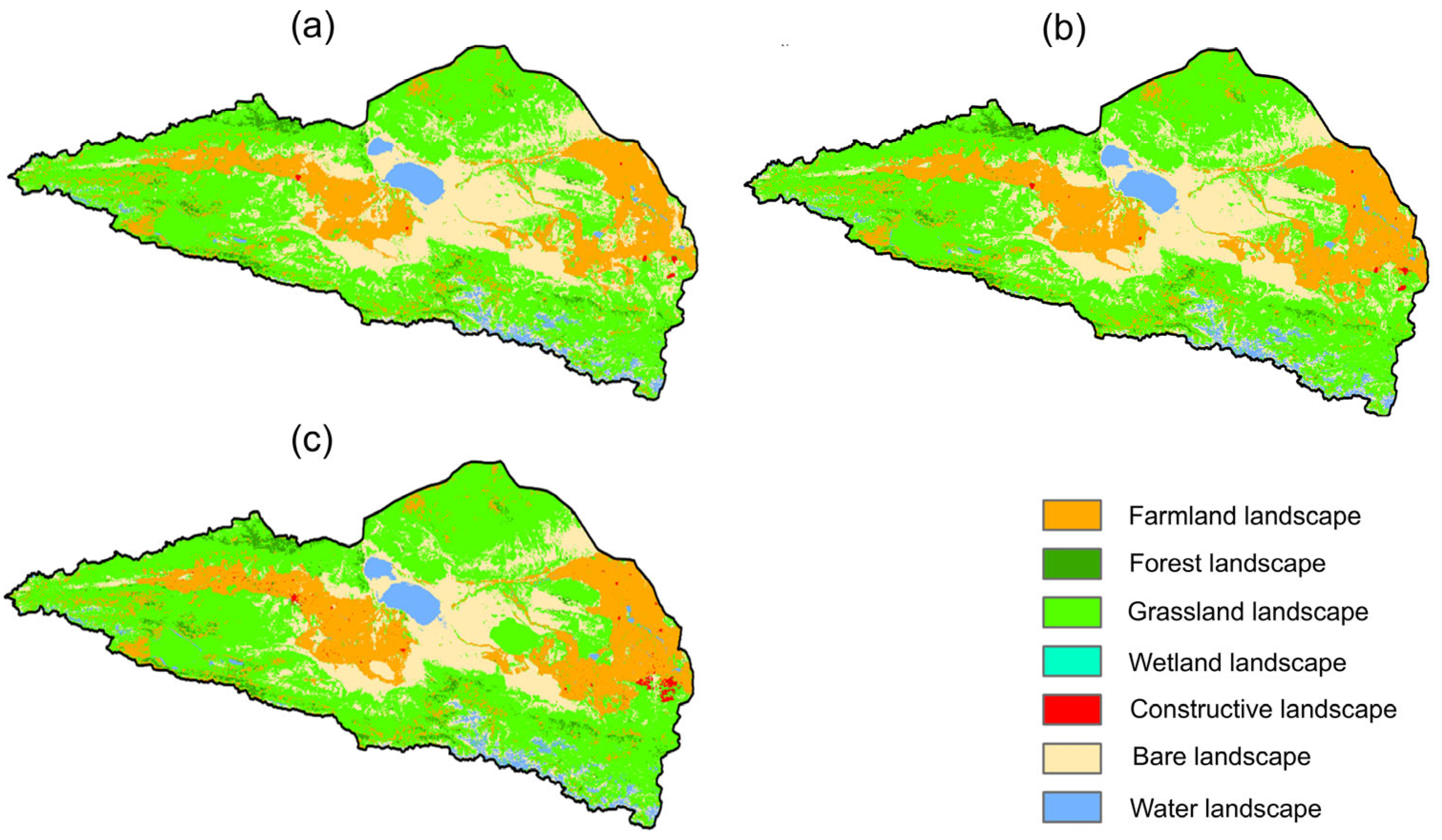
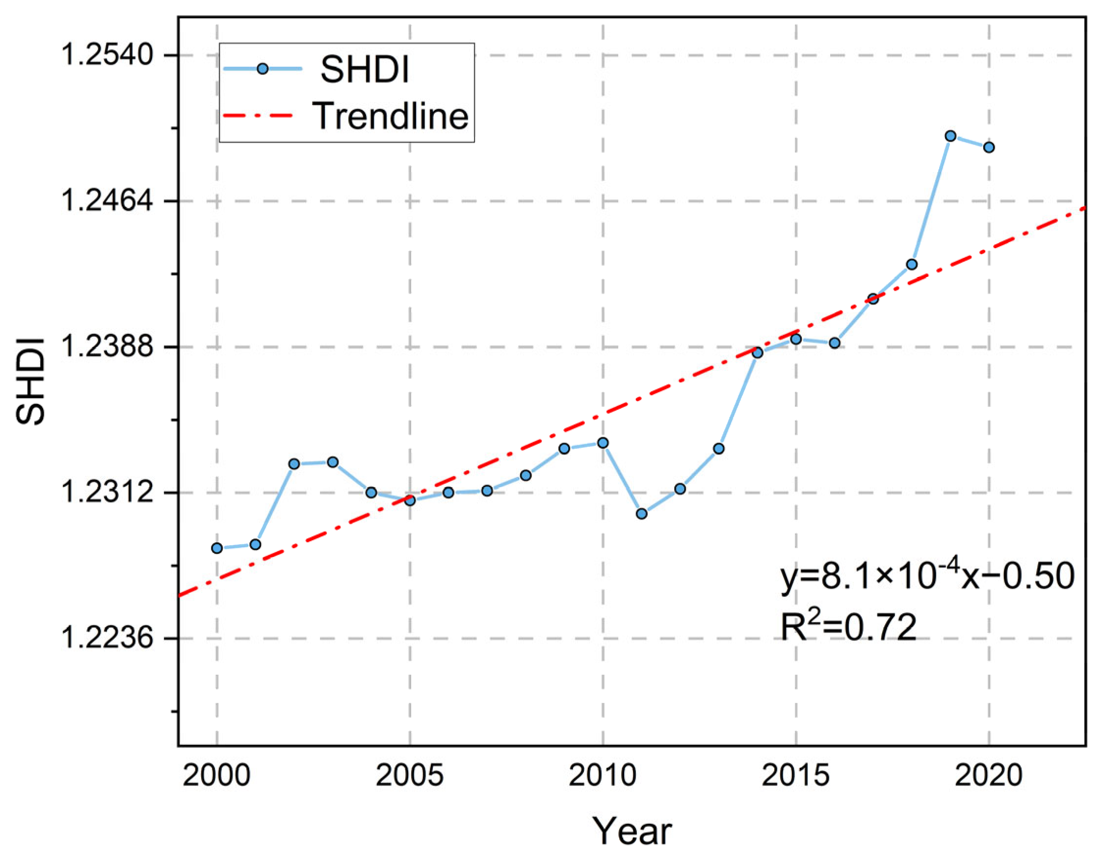
3.1. Spatiotemporal Changes in Landscape Patterns

Based on the temporal variations in the NP and PD for each landscape type in the ELB from 2000 to 2020, the landscape patterns of different land use types in the basin exhibited clear spatiotemporal differences (

Table 2. Table of changes in NP and PD for land use types in the ELB.

Landscape Type	2000		2010		2020
	NP	PD	NP	PD	NP	PD
Farmland Landscape	2048	0.0438	1828	0.0391	1868	0.0399
Forest Landscape	794	0.0170	763	0.0163	954	0.0204
Grassland Landscape	1700	0.0363	1594	0.0341	1648	0.0352
Wetland Landscape	13	0.0003	13	0.0003	15	0.0003
Constructive Landscape	8	0.0002	68	0.0015	253	0.0054
Bare Landscape	2710	0.0579	2693	0.0576	2647	0.0566
Water Landscape	412	0.0088	422	0.0090	444	0.0095

). Overall, the NP and PD of cropland areas continuously decreased, indicating that the distribution of cropland areas was shifting from fragmented to large-scale and contiguous patterns, with small-scale croplands gradually merging to form larger continuous areas. The NP of forest landscapes slightly increased, accompanied by a relatively small increase in PD, indicating, on one hand, a partial restoration or expansion of forest areas in local sub-basins, and on the other hand, due to the linear distribution of forests along riversides and foothills, newly added patches were concentrated without demonstrating a significant fragmentation trend. The NP and PD of grassland landscapes fluctuated considerably in the early period, associated with the local conversion of grasslands to croplands or construction land. In the later period, these indices stabilized or slightly increased, indicating an increasingly concentrated distribution of grasslands. The NP and PD of wetland areas did not exhibit significant changes, being notably influenced by fluctuations in lake water levels and wetland conservation policies. During periods of wetland area expansion, the number and density of patches increased simultaneously, while declines occurred during droughts or periods of water scarcity. The NP and PD of construction land landscapes continuously increased, with particularly significant growth from 2000 to 2010, reflecting accelerated urbanization and infrastructure development. This indicates that construction land gradually exhibited a pattern characterized by numerous small patches. The NP and PD of bare land landscapes fluctuated during different periods due to natural drought, soil salinization, and conversions between bare land and cropland, forestland, or grassland. The NP and PD of water landscapes showed continuous growth from 2000 to 2020, mainly influenced by changes in the water level of Ebinur Lake and seasonal hydrological processes. During periods of favorable hydrological conditions or rational water allocation, the number and density of water patches increased, whereas they correspondingly decreased during drought periods. Overall, the evolution of patch patterns across various landscape types in the ELB reflects the dynamic adjustment characteristics of landscape patterns under the combined influences of natural environmental changes and human activities.

From 2000 to 2020, the Landscape Shape Index (LSI) and Perimeter–Area Fractal Dimension (PAFRAC) of various landscape types in the ELB generally evolved from relatively regular to more complex and diverse patterns (

Table 3. Table of changes in LSI and PAFRAC for land use types in the ELB.

Landscape Type	2000		2010		2020
	LSI	PAFRAC	LSI	PAFRAC	LSI	PAFRAC
Farmland Landscape	40.9790	1.4630	36.3653	1.4726	37.8435	1.4708
Forest Landscape	37.4745	1.4930	36.5879	1.4934	41.0463	1.4936
Grassland Landscape	61.5392	1.4859	58.2641	1.4882	56.2352	1.4944
Wetland Landscape	5.0000	1.5421	5.0000	1.5421	5.0833	1.5565
Constructive Landscape	3.1778	1.0460	7.1296	1.2428	15.7835	1.3814
Bare Landscape	61.1496	1.4913	57.3669	1.4989	53.9501	1.4951
Water Landscape	21.8770	1.4246	21.8949	1.4221	22.2229	1.4130

). The LSI of cropland areas showed an overall decline, decreasing from 40.98 in 2000 to 37.84 in 2020, while the PAFRAC slightly increased from 1.46 to 1.47. This indicates that, during the processes of land consolidation and expansion, cropland patch sizes decreased and their boundaries became more irregular and complex. The LSI of forest landscapes increased from 37.48 to 41.05, while the rise in the PAFRAC was relatively moderate, indicating that forests are primarily distributed in linear patterns along foothills or riverbanks, with an overall low degree of fragmentation. During this period, the LSI of grassland landscapes fluctuated slightly from 61.54 to 56.24, and the PAFRAC showed minimal change, indicating localized degradation and increased fragmentation of grasslands. The PAFRAC of wetland areas slightly increased from 1.54 in 2000 to 1.56 in 2020, indicating greater boundary complexity, mainly influenced by fluctuations in lake water levels or ecological conservation efforts. The LSI and PAFRAC of construction land landscapes increased significantly, with the LSI rising from 3.18 to 15.78 and the PAFRAC from 1.05 to 1.38, reflecting land sprawl and fragmentation driven by rapid urbanization and infrastructure expansion. The LSI of bare land landscapes decreased from 61.15 to 53.95, while the PAFRAC remained relatively stable, indicating that natural processes such as drought and salinization, along with conversions between bare land and cropland, forestland, or grassland, have collectively contributed to increasingly irregular patch shapes. The LSI of water body landscapes showed little change, while the PAFRAC decreased slightly from 1.43 to 1.41, indicating a trend toward shoreline simplification. Overall, the various landscape types in the ELB have generally undergone a spatial reorganization process over the past 30 years, shifting from concentrated and regular patterns to more complex and diverse configurations. This transformation reflects both the impacts of natural environmental changes and the profound reshaping of landscape patterns by human activities.

From a spatial perspective, the ELB exhibits an overall elongated distribution along the east–west axis, with significant spatial differentiation among different land use types (Figure 3). Croplands are primarily concentrated in the flat alluvial plains of the eastern and southeastern parts of the basin, exhibiting a continuous and clustered distribution with high density, and their expansion across the basin is clearly observable. In contrast, croplands in the western and northern parts of the basin are more scattered and relatively smaller in the area. Forests are mainly distributed along the basin margins and foothill transition zones, typically in linear or patchy mosaic patterns, corresponding to higher elevation areas within the basin. Grasslands have the widest coverage, primarily concentrated in the broad, mid- to low-elevation areas of the basin. They are distributed in large, continuous patches with lower density compared to croplands in the eastern region, but they span a vast area. Wetlands are mostly distributed along lake shores and major riverbanks, generally small in scale, and appear as patchy or linear mosaics embedded among other land use types. Construction land is mainly concentrated along major transportation routes and around urban areas. Although it occupies a small proportion of the entire basin, it has expanded rapidly within urban zones and economic corridors, exhibiting a clear pattern of spatial agglomeration. Bare land is widely distributed in the central and northwestern parts of the basin, closely corresponding to arid climatic conditions and areas of severe salinization, and is often interspersed with grasslands and forests. Water bodies are mainly concentrated in the Ebinur Lake area and its surroundings, forming a composite pattern composed of large lake basins and multiple small water patches. Overall, the southeastern part of the basin is dominated by cropland, while the central and northwestern regions are primarily composed of bare land and grassland. Wetlands and water bodies are concentrated in the central lake area and its surroundings, forests are distributed in linear patterns along the foothills, and construction land is mainly distributed in linear or clustered forms around major towns and transportation hubs.

From 2000 to 2020, the Shannon Diversity Index (SHDI) of the ELB showed a steady upward trend (Figure 4). The relatively high $R_{SHDI}^2$ value indicates a strong positive correlation between the Shannon Index and time. The SHDI increased from approximately 1.228 in 2000 to around 1.254 in 2020, suggesting improvements in both the richness and evenness of land use types within the basin. This upward trend reflects a shift in landscape structure from relatively homogeneous to more diverse patterns. Specifically, from 2000 to 2010, the rapid expansion of construction land and the dynamic changes in wetland patterns significantly increased landscape fragmentation and heterogeneity, driving a continuous rise in the SHDI. Between 2010 and 2015, although the SHDI exhibited only slight fluctuations with limited growth, the SHDI showed a slow increase due to the combined effects of cropland expansion, localized forest restoration, and grassland degradation. Since 2015, the growth momentum of the SHDI has accelerated further, reaching its highest level by 2020. During this period, changes in the spatiotemporal distribution of water bodies and the ongoing urbanization process jointly contributed to an increasingly complex and diverse landscape pattern within the basin. Overall, under the combined influence of natural processes and human activities, the SHDI in the ELB has continued to increase, reflecting the ongoing differentiation and reorganization of ecosystem structure and function.

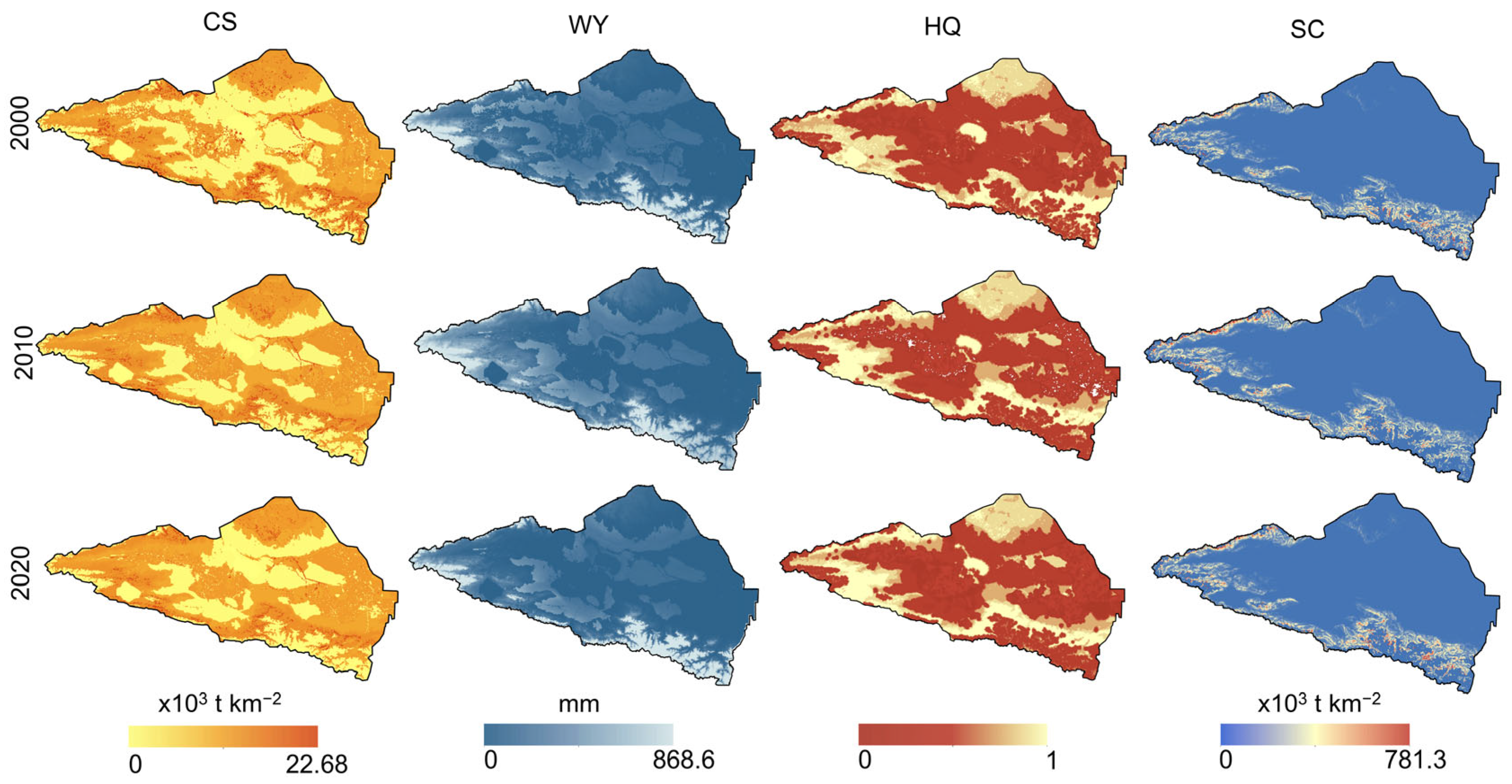
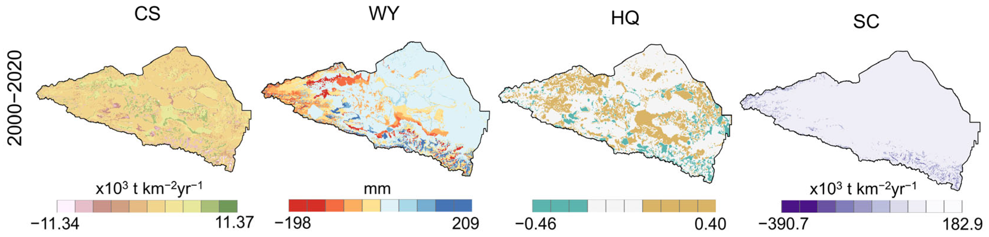
3.2. Spatiotemporal Changes in Ecosystem Services

From 2000 to 2020, ESs in the ELB exhibited varying changes over time (

Table 4. Temporal changes of four indicators of ecosystem services in the ELB.

	CS (102 t)	HQ	SC (103 t)	WY (mm)
2000	83.07	0.47	16.17	79.31
2010	89.21	0.48	19.87	115.99
2020	89.38	0.48	13.12	61.38

). Carbon sequestration (CS) showed an overall upward trend, increasing from 83.07 × 10² t in 2000 to 89.38 × 10² t in 2020. Habitat quality (HQ) remained relatively stable, with a slight increase from 2000 to 2010, followed by a plateau. Soil retention (SC) fluctuated between 2000 and 2020, reaching a peak of 19.87 × 10³ t in 2010 and then declining to its lowest value of 13.12 × 10³ t by 2020. Water yield (WY) experienced significant fluctuations from 2000 to 2020, reaching its highest value of 115.99 mm in 2010 and dropping to a minimum of 61.38 mm by 2020.

From 2000 to 2020, ESs in the ELB underwent various changes across the spatial dimension, with different service functions exhibiting distinct spatial heterogeneity across sub-basins (Figure 5 and Figure 6). Carbon sequestration was largely stable throughout the basin, with minor reductions observed in several central-western and southern sub-basins, likely driven by changes in land use or diminished vegetation density. The general trend indicated a minor reduction in habitat quality, especially concentrated in the central and southern parts of the ELB, where spatial variation trends indicate significant habitat degradation. After 2010, a pronounced decline in soil retention was observed in the western and southern parts of the basin, suggesting an escalation in soil erosion processes. Water yield showed substantial spatial and temporal variation, with a notable decline in the southeastern and western regions after 2010, likely driven by decreased precipitation or shifts in water resource management practices.

3.3. Assessment of Comprehensive Ecosystem Service Benefits

From 2000 to 2020, the comprehensive ES benefits in the ELB exhibited dynamic spatial changes (Figure 7). Overall, during this 20-year period, the spatial distribution of comprehensive benefits showed fluctuations in the central-southern, northwestern, and eastern regions of the ELB. The central-southern region of the ELB exhibited relatively high comprehensive benefits due to extensive vegetation cover and effective management policies. Although the overall distribution pattern of ES benefits changed in 2000, the central region still maintained a high level of comprehensive benefits. Due to natural factors such as drastic climate changes and the limited carrying capacity of ecosystems, the northwestern and eastern regions gradually exhibited a declining trend in comprehensive benefits from 2000 to 2020. However, the overall magnitude of change remained relatively small.

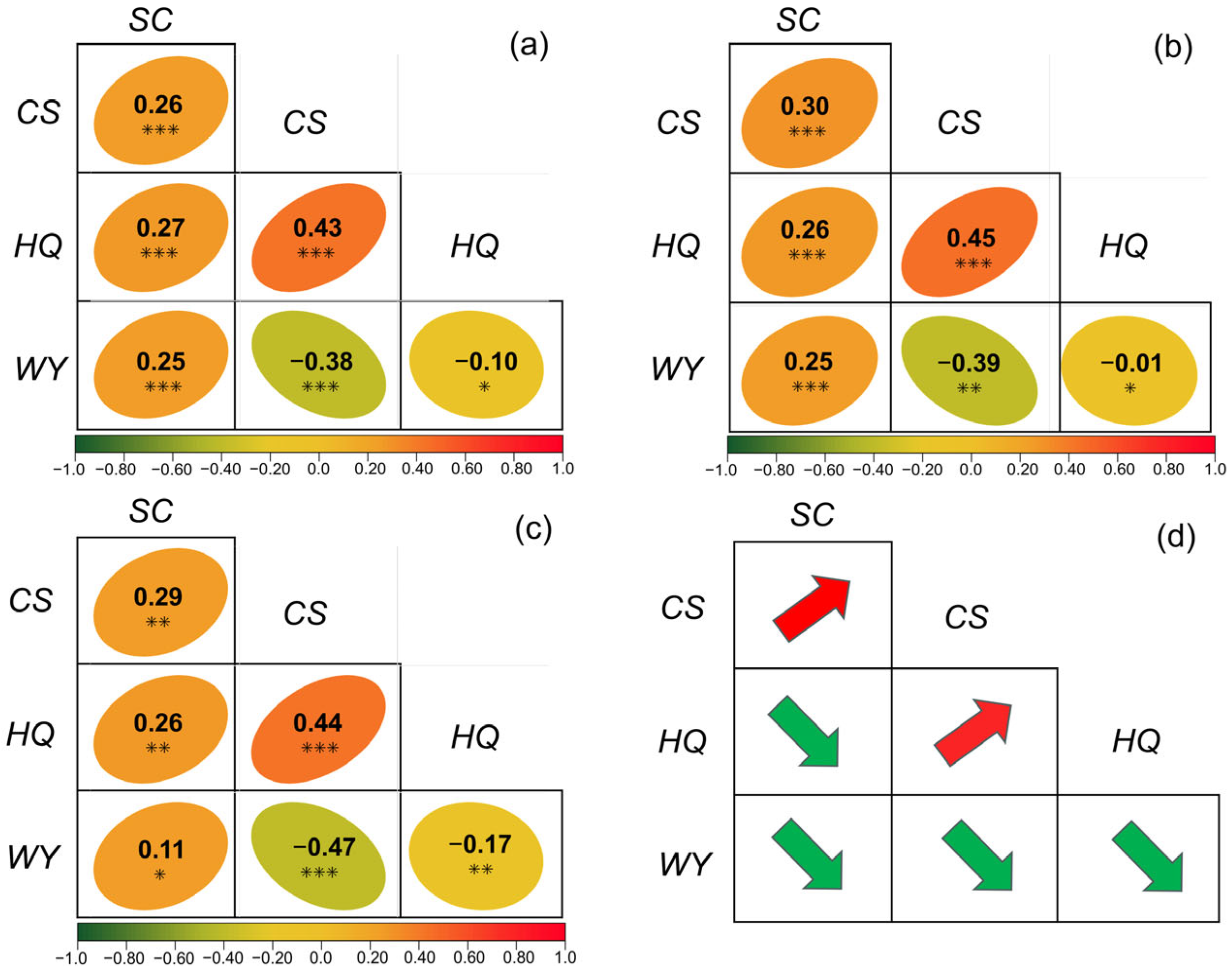
3.4. Trade-Offs and Synergies Among Ecosystem Services

From 2000 to 2020, ESs in the ELB exhibited a clear pattern of synergies (Figure 8), with the synergistic effect between carbon sequestration and habitat quality improvement being particularly prominent. Particularly in 2010, the enhancement of carbon sequestration capacity showed a strong positive correlation with improvements in habitat quality. This indicates that the expansion of vegetation covered not only effectively strengthened carbon fixation but also significantly improved habitat conditions while simultaneously enhancing soil retention functions. However, the relationship between habitat quality and water yield was relatively weak and even showed a certain degree of negative correlation, suggesting that increased vegetation cover may have exerted competitive pressure on water resources to some extent. Overall, ESs in the ELB were predominantly characterized by synergistic relationships.

4. Discussion

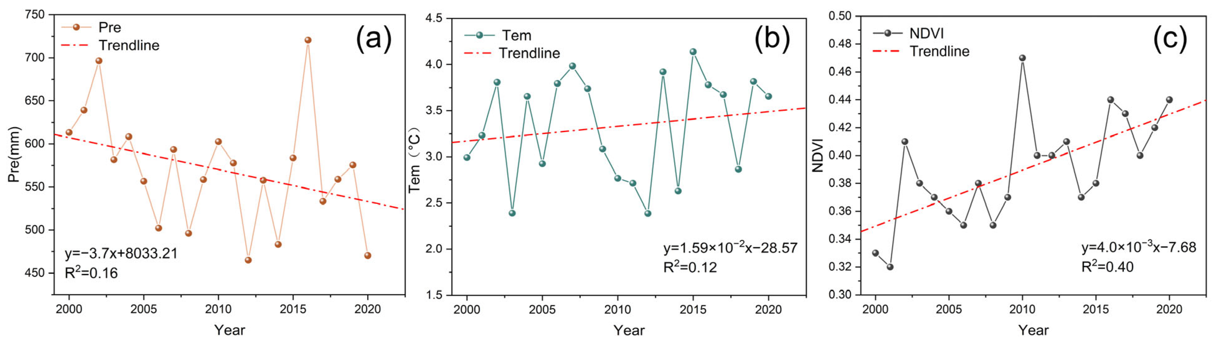
4.1. Influence of Natural Factors on Landscape Patterns

Landscape patterns describe the spatial arrangement and organization of landscape elements varying in type, size, and shape. They are typically quantified and compared using landscape indices, which are further used to analyze their relationships with ecosystem functions and services [70]. Landscape pattern indices can quantitatively characterize landscape heterogeneity, fragmentation, and connectivity, and they are of great significance for evaluating ecological processes [71]. In general, natural factors—such as temperature (Tem), precipitation (Pre), and vegetation cover—affect landscape patterns primarily by altering vegetation growth and distribution patterns, thereby influencing the spatial composition and dynamics of LULC types. Tem and Pre together determine the moisture and energy conditions within the basin and often influence patch number, density, connectivity, and shape complexity across different temporal scales [72]. Vegetation cover further reveals the impact of natural environmental changes on the evolution of patch fragmentation and heterogeneity. Drought or extreme weather events often lead to fluctuations in patch numbers, increased landscape fragmentation, or reduced connectivity [73]. This has a significant negative impact on the ecosystem functions and services of the basin. As shown in the time series results from 2000 to 2020 (Figure 9), under the influence of arid region climate characteristics, Pre in the study basin exhibited an overall fluctuating decline, while Tem slowly increased, creating a dual stress pattern of “decreasing Pre-rising Tem“. However, the NDVI continuously increased during this period, indicating that, despite overall water scarcity and rising Tem, vegetation cover and growth conditions in the basin still showed some degree of improvement. Further correlation analysis between natural factors and time revealed that the time series correlations of Pre and Tem ($R_{Pre}^2$ and $R_{Tem}^2)$ were both relatively low, indicating that their temporal fluctuations had a minimal direct impact on landscape fragmentation and other related indices. However, the $R_{NDVI}^2$ value reached 0.43, reflecting a significant improvement in vegetation cover over time during this period. This also suggests that the rise in Tem and the extension of the growing season had a positive effect on vegetation growth under certain local conditions, leading to phased changes in landscape patch number, density, boundary complexity, and fragmentation. In a study on landscape pattern changes in the Xiliao River Plain of the northwestern semi-arid region, it was similarly found that the dynamic changes in landscape patterns were less influenced by natural factors [74], which is in line with the results of this study. However, this study also found that the ELB’s wetland ecosystems are crucial for water conservation, ecological regulation, and biodiversity protection, making them essential for the basin’s sustainable development. Wetlands play an irreplaceable key role in water conservation, pollutant degradation, carbon sequestration, and habitat provision. Their landscape pattern directly determines the effectiveness of wetland ecosystem functions. Once wetland areas become fragmented, their flood regulation and water purification functions are significantly weakened. When Tem increases in conjunction with other factors, such as water level declines caused by higher evaporation, shallow wetland areas are more prone to reduction. This leads to the expansion of bare land or low-coverage areas, accelerating wetland patch fragmentation and simplifying functional communities. In arid or semi-arid regions, if Pre continues to decrease and Tem rise, wetland patches are more likely to be disturbed and fragmented, further intensifying fragmentation [75]. This has adverse effects on species diversity, nutrient cycling, and overall ES functions. The spatiotemporal variations in natural environmental factors (such as Tem, Pre, and vegetation cover) not only affect landscape pattern indices, such as wetland patch number, density, and boundary shape but also play a crucial regulatory role in the health and service functions of wetland ecosystems [76]. This issue requires sustained and in-depth attention in future research and management efforts.

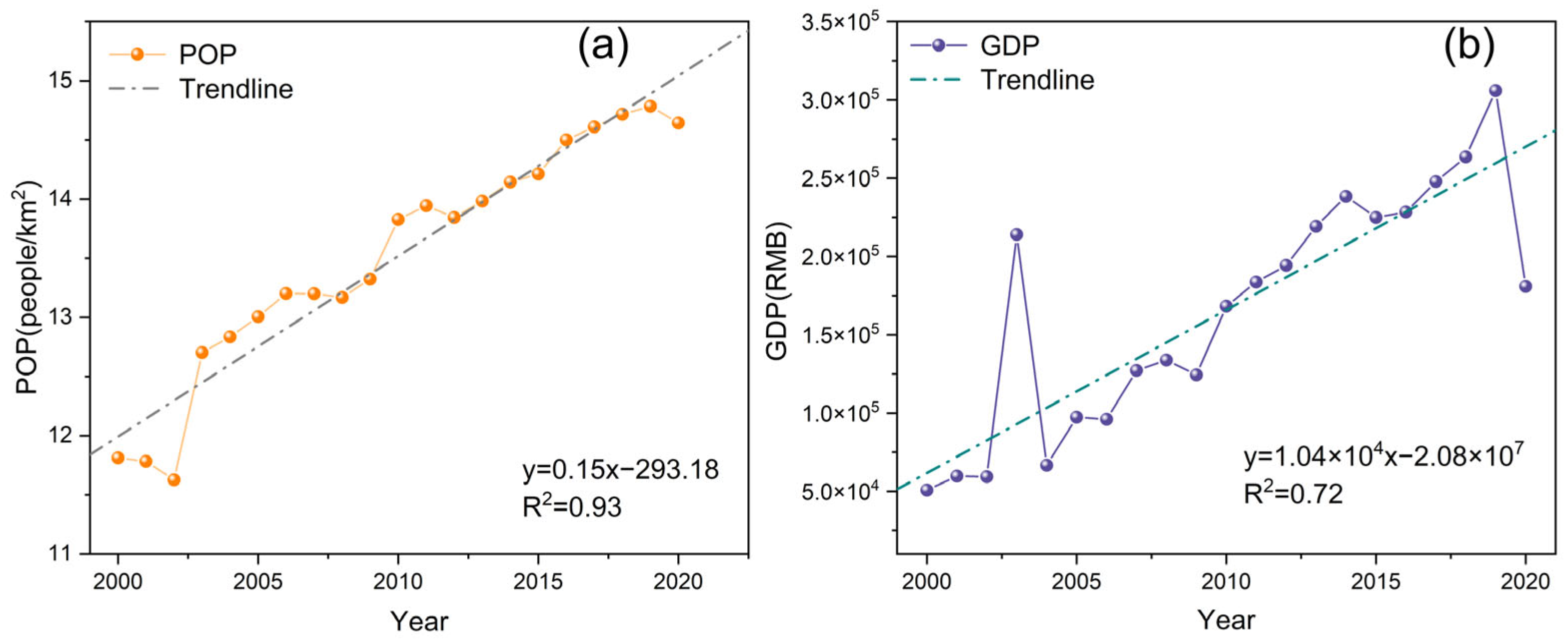
4.2. Influence of Anthropogenic Factors on Landscape Patterns

Under the growing influence of anthropogenic factors on the natural environment, changes in landscape patterns have become increasingly complex [77]. From 2000 to 2020, both POP and per capita GDP in the ELB showed a continuous and rapid upward trend (Figure 10). The high values of $R_{pop}^2$ and $R_{GDP}^2$ indicate a significant positive correlation between POP, per capita GDP, and time. This phenomenon highlights the profound influence of intensified human activities on landscape patterns within the basin, indicating that anthropogenic factors are the primary driving force behind landscape pattern changes. A study on forest landscape changes in central-western Alberta, Canada, similarly indicated that human activities are the root cause of contemporary landscape changes [78]. This study found that the continuous growth of the basin’s population and the improvement in economic levels directly influenced changes in land use and spatial structure. First, an increase in population size typically signifies intensified human activity, often leading to the rapid expansion of construction land, transportation networks, and agricultural land. This, in turn, results in the fragmentation or direct occupation of original natural landscapes such as grasslands, forests, and wetlands. This process generally leads to an increase in the number and density of patches, thereby intensifying landscape fragmentation. Second, the growth of per capita GDP typically reflects an improvement in economic development, which not only accelerates urbanization and infrastructure construction but also increases investment in environmental protection and ecological restoration. As a result, landscape evolution within the basin exhibits distinct differentiation patterns [79]. For example, construction land has rapidly expanded in economic core areas and along transportation corridors, leading to increased boundary complexity [80]. In some basins where ecological management has received greater attention, there has been a concentrated and large-scale restoration of forest and grassland areas, resulting in a relative reduction in landscape fragmentation. This indicates that different stages of economic development and basin-specific conditions have complex effects on landscape patterns—both intensifying fragmentation and promoting landscape restoration and improvement [81]. The increase in POP and per capita GDP can, to some extent, intensify land demand and the expansion of economic activities, thereby exerting substantial impacts on landscape patterns [82]. Therefore, to achieve coordinated development between the economy and ecological protection, it is essential to implement scientific spatial planning and policy guidance to balance the relationship between economic growth and ecological security.

4.3. Influence of Natural Factors on Ecosystem Services

The ELB lies within an arid zone characterized by a highly vulnerable and sensitive ecological environment. Studying the impact of natural factors—such as Tem, Pre, and NDVI—on changes in ESs is of great practical significance and is crucial for ensuring the stable development of the basin’s socio-economic systems and the sustainability of its ecological environment [83]. Tem and Pre, as the primary natural factors, directly influence hydrothermal conditions and significantly affect ecosystem provisioning services by altering vegetation growth environments. Analyzing the correlation between climate and ES benefits in the basin indicates that climate change plays a decisive role in maintaining the stability of ESs and regulating trade-offs among them [84]. As a key indicator of vegetation growth, the NDVI reflects the dynamic changes in vegetation cover within the basin and plays an important role in local ESs [85]. Research shows that, under the combined influence of climate change and NDVI, the proportions of areas positively correlated with ESs in the ELB were 74% for Pre, 50% for Tem, and 52% for the NDVI (Figure 11). Under extreme climatic conditions in arid regions, Pre emerges as the primary driver shaping ES in the ELB. Tem and the NDVI also exert varying impacts on the basin, leading to a strong synergistic relationship between water yield and soil retention. Compared to other basins, the Yellow River Basin exhibits the most significant synergy between ESs such as soil retention and water yield [86], aligning well with the results of this study. This study found that the disruption of Pre stability has exacerbated water scarcity, thereby impacting the ecosystem’s water supply services. Rising Tem has a profound impact on the structure and distribution of biological communities, particularly leading to a reduction in the suitable habitat range for cold-tolerant plant species under a warming climate. Research shows that high NDVI values are mainly concentrated in mountainous areas and croplands, while low NDVI values are distributed in regions of desertification and salinization. Changes in plant community composition and growth cycles have led to a continuous decline in ES benefits as reflected by the NDVI. As key indicators of ESs in the basin, carbon sequestration and habitat quality are directly influenced by climatic factors and the NDVI. Changes in climate and the NDVI significantly affect the growth of herbaceous plants and root biomass, thereby impacting ESs. In addition, Tem variations affect soil moisture through evaporation and freezing processes, thereby indirectly influencing soil retention capacity, while changes in Pre amount and intensity directly determine the water yield services of the ELB [87]. Therefore, in ecosystem management, it is essential to conduct an in-depth analysis of the relationship between climate variables and the NDVI to optimize the provision of ESs. To safeguard the ecological integrity and long-term resilience of the basin’s ecosystem, differentiated management strategies should be adopted, with refined management approaches aimed at maximizing ES benefits.

4.4. Influence of Anthropogenic Factors on Ecosystem Services

Changes in ESs induced by human activities further affect the intrinsic relationships among different ESs [88]. With the intensification of human activities, ecosystems have undergone significant changes, leading to the pollution and degradation of soil, air, and water resources, resulting in a marked impact on the value of ESs [89]. Through analysis of the total value of ESs and the value of various service types, it was found that per capita GDP and POP are key factors driving changes in the total value of ESs, as well as in the values of regulating and supporting services. Research shows that the proportion of areas positively correlated with ESs in the ELB was 33% for POP and 70% for per capita GDP (Figure 12). In the ELB, POP shows a weak positive correlation with ESs. In particular, areas with high POP have experienced significant declines in biodiversity and wetland area, as well as weakened climate regulation capacity, resulting in trade-offs among ESs. Per capita GDP shows a strong coupling relationship with ESs. As the economy grows rapidly, the government has implemented a series of optimization policies that promote wetland restoration, soil and water conservation, and consequently enhance ESs. Compared with ecosystems in other study regions, the trade-offs and synergies among ESs in the ELB exhibit both similarities and differences. The trade-offs and synergies among EPLFs (Ecosystem Production and Life-supporting Functions) in the Qilian Mountain grasslands exhibit significant spatiotemporal variations [90]. Due to the continuous increase in POP and per capita GDP, grassland resources have been overexploited, resulting in a general trend where trade-offs far outweigh synergies—consistent with the findings of this study. However, the relatively low level of human disturbance in the Tianshan Mountains has fostered positive interactions among ESs, promoting the formation of synergies [91]. This study also found that POP and economic growth in the ELB have driven increased land demand, particularly in urban and oasis areas, leading to the conversion of large areas of natural land into agricultural and construction land. To meet food demand, cropland has been continuously expanded, reducing natural vegetation cover and consequently affecting ESs such as soil retention and water supply. Changes in water yield further affect habitat quality and carbon sequestration functions, resulting in feedback effects among ESs. These changes, in turn, influence the trade-offs and synergies among ESs [92]. Thus, the observed trade-offs and synergies among ecosystem services in the ELB are indicative of the region’s distinct ecological conditions and resource management strategies, indicating that the interactions among ESs exhibit distinct characteristics across different basins and contexts.

4.5. Prospects and Limitations

This study advances the understanding of ecosystem service dynamics in arid terminal lake basins, a landscape type underrepresented in global ES research. By integrating landscape pattern indices with InVEST modeling, we link spatial configuration with functional service flows. Standardized indicators and trade-off–synergy analysis enhance temporal comparability. This study also identifies threshold responses of fragmentation and service supply to combined climatic and socio-economic drivers, offering a replicable framework for assessing ES resilience in fragile inland ecosystems. This study established a multi-scale, multi-dimensional analytical framework and revealed the mechanisms of landscape and ES evolution in the ELB. However, there is still room for improvement. The current data are mainly derived from remote sensing imagery and statistical yearbooks, whose spatial and temporal resolution and update frequency are insufficient to meet the requirements of high-precision simulations [93]. In the future, high-resolution satellite imagery and UAV aerial surveys should be employed to improve the accuracy and timeliness of model inputs [94]. Secondly, the ES assessment in this study relies on landscape pattern indices and the InVEST model, which simplifies the coupling processes of water–carbon–habitat–soil systems. In the future, integrating process-based models with machine learning techniques could enable more refined predictions of ecosystem provisioning and human activity responses [95]. In addition, this study preliminarily explored the trade-offs and synergies among ESs and quantified the comprehensive benefits of different land use scenarios in terms of carbon sequestration, habitat conservation, water yield, and soil retention. However, it lacks systematic scenario simulation, cost–benefit analysis, and the development of scenario-based decision support tools. Future research should integrate scenario simulations with multi-model ensembles to further quantify the comprehensive benefits of ESs [96]. This study revealed the significant impacts of driving factors such as Tem, Pre, the NDVI, POP, and per capita GDP through factor analysis. However, the causal pathways and threshold effects of these factors have not yet been clarified. Future work should further quantify nonlinear responses and identify critical thresholds to provide a scientific basis for differentiated management policies [97]. Finally, this study did not fully account for the uncertainties associated with future climate change and socio-economic scenarios. Long-term evolution forecasting and risk assessment should be conducted to provide forward-looking guidance for basin resilience building and adaptive management [98]. Through these improvements, the research outcomes will gain greater depth and practical value, providing a solid foundation for sustainable development and ecological restoration in the ELB.

5. Conclusions

This study established a multi-scale, multi-dimensional quantitative analysis framework that integrated climate, Pre, and socio-economic factors. By selecting typical landscape types and key ES indicators—including carbon sequestration, water yield, soil retention, and habitat quality—and employing landscape pattern indices and ES models, this study systematically revealed the dynamic evolution of landscape structure and function in the ELB, as well as the underlying ecological mechanisms. It also examined the trade-offs and synergies among ESs under increasingly complex landscape conditions, thereby offering a scientific basis for water resource management and ecological restoration efforts in the basin.

This study shows that, from 2000 to 2020, cropland and construction land exhibited an expanding and fragmenting trend, while grasslands and wetlands generally shrank or experienced fluctuating degradation, leading to increasingly complex landscape boundaries. The ES assessment results indicate that carbon sequestration showed an overall increase, habitat quality slightly improved from 2000 to 2010 and then stabilized, and soil retention and water yield exhibited significant fluctuations, with water yield showing a marked decline after 2010. In terms of spatial distribution, carbon sequestration weakened in some sub-basins in the central-western and southern regions, while habitat quality and soil retention capacity declined in certain areas. Water yield also showed a decreasing trend in the southeastern and western parts of the basin. Further analysis revealed a strong positive correlation between carbon sequestration and habitat quality, indicating that vegetation expansion not only enhanced carbon fixation but also improved habitat conditions and soil retention. In contrast, the relationship between habitat quality and water yield was weak or even negative, suggesting that increased vegetation may compete with water resources. In addition, Tem, Pre, the NDVI, POP, and per capita GDP all had significant impacts on landscape patterns and ESs. In summary, fully accounting for both natural and anthropogenic factors is of great significance for optimizing management policies and promoting the sustainable development of ESs in the ELB.

References

1. Danley, B.; Widmark, C. Evaluating conceptual definitions of ecosystem services and their implications. Ecol. Econ. 2016, 126, 132–138. [Google Scholar] [CrossRef]
2. Hernández-Blanco, M.; Costanza, R.; Chen, H.; DeGroot, D.; Jarvis, D.; Kubiszewski, I.; Montoya, J.; Sangha, K.; Stoeckl, N.; Turner, K. Ecosystem health, ecosystem services, and the well-being of humans and the rest of nature. Glob. Change Biol. 2022, 28, 5027–5040. [Google Scholar] [CrossRef] [PubMed]
3. Schirpke, U.; Wang, G.; Padoa-Schioppa, E. Mountain landscapes: Protected areas, ecosystem services, and future challenges. Ecosyst. Serv. 2021, 49, 101302. [Google Scholar] [CrossRef]
4. Fang, Z.; Ding, T.; Chen, J.; Xue, S.; Zhou, Q.; Wang, Y.; Wang, Y.; Huang, Z.; Yang, S. Impacts of land use/land cover changes on ecosystem services in ecologically fragile regions. Sci. Total Environ. 2022, 831, 154967. [Google Scholar] [CrossRef]
5. Hernández, R.C.; Camerin, F. The application of ecosystem assessments in land use planning: A case study for supporting decisions toward ecosystem protection. Futures 2024, 161, 103399. [Google Scholar] [CrossRef]
6. Allan, J.I.; Auld, G.; Cadman, T.; Stevenson, H. Comparative fortunes of ecosystem services as an international governance concept. Glob. Policy 2022, 13, 62–75. [Google Scholar] [CrossRef]
7. Peng, K.; Jiang, W.; Ling, Z.; Hou, P.; Deng, Y. Evaluating the potential impacts of land use changes on ecosystem service value under multiple scenarios in support of SDG reporting: A case study of the Wuhan urban agglomeration. J. Clean. Prod. 2021, 307, 127321. [Google Scholar] [CrossRef]
8. Zhang, H.; Zhang, Z.; Liu, K.; Huang, C.; Dong, G. Integrating land use management with trade-offs between ecosystem services: A framework and application. Ecol. Indic. 2023, 149, 110193. [Google Scholar] [CrossRef]
9. Wang, H.; Zhou, S.; Li, X.; Liu, H.; Chi, D.; Xu, K. The influence of climate change and human activities on ecosystem service value. Ecol. Eng. 2016, 87, 224–239. [Google Scholar] [CrossRef]
10. Wang, J.; Wu, W.; Yang, M.; Gao, Y.; Shao, J.; Yang, W.; Ma, G.; Yu, F.; Yao, N.; Jiang, H. Exploring the complex trade-offs and synergies of global ecosystem services. Environ. Sci. Ecotechnol. 2024, 21, 100391. [Google Scholar] [CrossRef]
11. Bai, Y.; Zhuang, C.; Ouyang, Z.; Zheng, H.; Jiang, B. Spatial characteristics between biodiversity and ecosystem services in a human-dominated watershed. Ecol. Complex. 2011, 8, 177–183. [Google Scholar] [CrossRef]
12. Li, B.; Wang, W. Trade-offs and synergies in ecosystem services for the Yinchuan Basin in China. Ecol. Indic. 2018, 84, 837–846. [Google Scholar] [CrossRef]
13. Bennett, E.M.; Peterson, G.D.; Gordon, L.J. Understanding relationships among multiple ecosystem services. Ecol. Lett. 2009, 12, 1394–1404. [Google Scholar] [CrossRef] [PubMed]
14. Troell, M.; Costa-Pierce, B.; Stead, S.; Cottrell, R.S.; Brugere, C.; Farmery, A.K.; Little, D.C.; Strand, Å.; Pullin, R.; Soto, D. Perspectives on aquaculture’s contribution to the Sustainable Development Goals for improved human and planetary health. J. World Aquac. Soc. 2023, 54, 251–342. [Google Scholar] [CrossRef]
15. Xia, H.; Yuan, S.; Prishchepov, A.V. Spatial-temporal heterogeneity of ecosystem service interactions and their social-ecological drivers: Implications for spatial planning and management. Resour. Conserv. Recycl. 2023, 189, 106767. [Google Scholar] [CrossRef]
16. Wang, B.; Zhang, Q.; Cui, F. Scientific research on ecosystem services and human well-being: A bibliometric analysis. Ecol. Indic. 2021, 125, 107449. [Google Scholar] [CrossRef]
17. Zeng, J.; Xu, J.; Li, W.; Dai, X.; Zhou, J.; Shan, Y.; Zhang, J.; Li, W.; Lu, H.; Ye, Y. Evaluating trade-off and synergies of ecosystem services values of a representative resources-based urban ecosystem: A coupled modeling framework applied to Panzhihua City, China. Remote Sens. 2022, 14, 5282. [Google Scholar] [CrossRef]
18. Wanghe, K.; Guo, X.; Ahmad, S.; Tian, F.; Nabi, G.; Strelnikov, I.I.; Li, K.; Zhao, K. FRESF model: An ArcGIS toolbox for rapid assessment of the supply, demand, and flow of flood regulation ecosystem services. Ecol. Indic. 2022, 143, 109264. [Google Scholar] [CrossRef]
19. Uniyal, B.; Kosatica, E.; Koellner, T. Spatial and temporal variability of climate change impacts on ecosystem services in small agricultural catchments using the Soil and Water Assessment Tool (SWAT). Sci. Total Environ. 2023, 875, 162520. [Google Scholar] [CrossRef]
20. Zhao, L.; Yu, W.; Meng, P.; Zhang, J.; Zhang, J. InVEST model analysis of the impacts of land use change on landscape pattern and habitat quality in the Xiaolangdi Reservoir area of the Yellow River basin, China. Land Degrad. Dev. 2022, 33, 2870–2884. [Google Scholar] [CrossRef]
21. Zafar, Z.; Zubair, M.; Zha, Y.; Mehmood, M.S.; Rehman, A.; Fahd, S.; Nadeem, A.A. Predictive modeling of regional carbon storage dynamics in response to land use/land cover changes: An InVEST-based analysis. Ecol. Inform. 2024, 82, 102701. [Google Scholar] [CrossRef]
22. Zhang, Y.; Guan, D.; Wu, L.; Su, X.; Zhou, L.; Peng, G. How can an ecological compensation threshold be determined? A discriminant model integrating the minimum data approach and the most appropriate land use scenarios. Sci. Total Environ. 2022, 852, 158377. [Google Scholar] [CrossRef]
23. Nguyen, T.T.; Grote, U.; Neubacher, F.; Do, M.H.; Paudel, G.P. Security risks from climate change and environmental degradation: Implications for sustainable land use transformation in the Global South. Curr. Opin. Environ. Sustain. 2023, 63, 101322. [Google Scholar] [CrossRef]
24. Terrado, M.; Sabater, S.; Chaplin-Kramer, B.; Mandle, L.; Ziv, G.; Acuña, V. Model development for the assessment of terrestrial and aquatic habitat quality in conservation planning. Sci. Total Environ. 2016, 540, 63–70. [Google Scholar] [CrossRef]
25. Martinez-Harms, M.J.; Bryan, B.A.; Balvanera, P.; Law, E.A.; Rhodes, J.R.; Possingham, H.P.; Wilson, K.A. Making decisions for managing ecosystem services. Biol. Conserv. 2015, 184, 229–238. [Google Scholar] [CrossRef]
26. Wong, C.P.; Jiang, B.; Kinzig, A.P.; Lee, K.N.; Ouyang, Z. Linking ecosystem characteristics to final ecosystem services for public policy. Ecol. Lett. 2015, 18, 108–118. [Google Scholar] [CrossRef]
27. Yue, L.; Shi, Q.; Jingjing, L. Research on ecological restoration technology in arid or semi-arid areas from the perspective of the Belt and Road Initiative. J. Resour. Ecol. 2022, 13, 964–976. [Google Scholar] [CrossRef]
28. Chen, X.; Wang, Y.; Pei, H.; Guo, Y.; Zhang, J.; Shen, Y. Expansion of irrigation led to inland lake shrinking in semi-arid agro-pastoral region, China: A case study of Chahannur Lake. J. Hydrol. Reg. Stud. 2022, 41, 101086. [Google Scholar] [CrossRef]
29. Guo, C.; Gao, J.; Zhou, B.; Yang, J. Factors of the ecosystem service value in water conservation areas considering the natural environment and human activities: A case study of Funiu mountain, China. Int. J. Environ. Res. Public Health 2021, 18, 11074. [Google Scholar] [CrossRef]
30. Fischer, G.; Tubiello, F.N.; Van Velthuizen, H.; Wiberg, D.A. Climate change impacts on irrigation water requirements: Effects of mitigation, 1990–2080. Technol. Forecast. Soc. Change 2007, 74, 1083–1107. [Google Scholar] [CrossRef]
31. Alizadeh-Choobari, O.; Ahmadi-Givi, F.; Mirzaei, N.; Owlad, E. Climate change and anthropogenic impacts on the rapid shrinkage of Lake Urmia. Int. J. Climatol. 2016, 36, 4276–4286. [Google Scholar] [CrossRef]
32. Xu, J.; Wang, Y.; Teng, M.; Wang, P.; Yan, Z.; Wang, H. Ecosystem services of lake-wetlands exhibit significant spatiotemporal heterogeneity and scale effects in a multi-lake megacity. Ecol. Indic. 2023, 154, 110843. [Google Scholar] [CrossRef]
33. Davis, M.D. Integrated water resource management and water sharing. J. Water Resour. Plan. Manag. 2007, 133, 427–445. [Google Scholar] [CrossRef]
34. Haddad, N.M.; Brudvig, L.A.; Clobert, J.; Davies, K.F.; Gonzalez, A.; Holt, R.D.; Lovejoy, T.E.; Sexton, J.O.; Austin, M.P.; Collins, C.D. Habitat fragmentation and its lasting impact on Earth’s ecosystems. Sci. Adv. 2015, 1, e1500052. [Google Scholar] [CrossRef] [PubMed]
35. Dobson, A.; Lodge, D.; Alder, J.; Cumming, G.S.; Keymer, J.; McGlade, J.; Mooney, H.; Rusak, J.A.; Sala, O.; Wolters, V. Habitat loss, trophic collapse, and the decline of ecosystem services. Ecology 2006, 87, 1915–1924. [Google Scholar] [CrossRef]
36. Luo, C.; Ma, X.; Yan, W.; Wang, Y. Trade-Offs and Optimization of Ecosystem Services in the Plain Terminal Lake Basin: A Case Study of Xinjiang. Land Degrad. Dev. 2024, 35, 5043–5061. [Google Scholar] [CrossRef]
37. Shen, Z.; Wu, W.; Tian, S.; Wang, J. A multi-scale analysis framework of different methods used in establishing ecological networks. Landsc. Urban Plan. 2022, 228, 104579. [Google Scholar] [CrossRef]
38. Andrew, M.E.; Wulder, M.A.; Nelson, T.A. Potential contributions of remote sensing to ecosystem service assessments. Prog. Phys. Geogr. 2014, 38, 328–353. [Google Scholar] [CrossRef]
39. Foroumandi, E.; Nourani, V.; Kantoush, S.A. Investigating the main reasons for the tragedy of large saline lakes: Drought, climate change, or anthropogenic activities? A call to action. J. Arid Environ. 2022, 196, 104652. [Google Scholar] [CrossRef]
40. Zhang, X.; Li, Y.; Ren, S.; Zhang, X. Soil CO2 emissions and water level response in an arid zone lake wetland under freeze–thaw action. J. Hydrol. 2023, 625, 130069. [Google Scholar] [CrossRef]
41. Qian, Y.; Wu, Z.; Zhang, L.; Zhou, H.; Wu, S.; Yang, Q. Eco-environmental evolution, control, and adjustment for Aibi Lake catchment. Environ. Manag. 2005, 36, 506–517. [Google Scholar] [CrossRef] [PubMed]
42. Srivastav, A.L.; Dhyani, R.; Ranjan, M.; Madhav, S.; Sillanpää, M. Climate-resilient strategies for sustainable management of water resources and agriculture. Environ. Sci. Pollut. Res. 2021, 28, 41576–41595. [Google Scholar] [CrossRef]
43. Pan, L.; Li, G.; Chen, C.; Liu, Y.; Lai, J.; Yang, J.; Jin, M.; Wang, Z.; Wang, X.; Ding, W. Late Holocene decoupling of lake and vegetation ecosystem in response to centennial-millennial climatic changes in arid Central Asia: A case study from Aibi Lake of western Junggar Basin. Palaeogeogr. Palaeoclimatol. Palaeoecol. 2024, 646, 112233. [Google Scholar] [CrossRef]
44. Rhodes, T.E.; Gasse, F.; Lin, R.; Fontes, J.-C.; Wei, K.; Bertrand, P.; Gibert, E.; Mélières, F.; Tucholka, P.; Wang, Z. A late pleistocene-Holocene lacustrine record from Lake Manas, Zunggar (northern Xinjiang, western China). Palaeogeogr. Palaeoclimatol. Palaeoecol. 1996, 120, 105–121. [Google Scholar] [CrossRef]
45. Zhaoyong, Z.; Xiaodong, Y.; Shengtian, Y. Heavy metal pollution assessment, source identification, and health risk evaluation in Aibi Lake of northwest China. Environ. Monit. Assess. 2018, 190, 1–13. [Google Scholar] [CrossRef] [PubMed]
46. Yao, J.; Mao, W.; Chen, J.; Dilinuer, T. Recent signal and impact of wet-to-dry climatic shift in Xinjiang, China. J. Geogr. Sci. 2021, 31, 1283–1298. [Google Scholar] [CrossRef]
47. Abahussain, A.A.; Abdu, A.S.; Al-Zubari, W.K.; El-Deen, N.A.; Abdul-Raheem, M. Desertification in the Arab Region: Analysis of current status and trends. J. Arid Environ. 2002, 51, 521–545. [Google Scholar] [CrossRef]
48. Alifujiang, Y.; Abuduwaili, J.; Ma, L.; Samat, A.; Groll, M. System dynamics modeling of water level variations of Lake Issyk-Kul, Kyrgyzstan. Water 2017, 9, 989. [Google Scholar] [CrossRef]
49. Zhao, Q.; Wen, Z.; Chen, S.; Ding, S.; Zhang, M. Quantifying land use/land cover and landscape pattern changes and impacts on ecosystem services. Int. J. Environ. Res. Public Health 2020, 17, 126. [Google Scholar] [CrossRef]
50. Peng, J.; Wang, Y.; Zhang, Y.; Wu, J.; Li, W.; Li, Y. Evaluating the effectiveness of landscape metrics in quantifying spatial patterns. Ecol. Indic. 2010, 10, 217–223. [Google Scholar] [CrossRef]
51. Plexida, S.G.; Sfougaris, A.I.; Ispikoudis, I.P.; Papanastasis, V.P. Selecting landscape metrics as indicators of spatial heterogeneity—A comparison among Greek landscapes. Int. J. Appl. Earth Obs. Geoinf. 2014, 26, 26–35. [Google Scholar] [CrossRef]
52. Chust, G.; Ducrot, D.; Pretus, J.L. Land cover mapping with patch-derived landscape indices. Landsc. Urban Plan. 2004, 69, 437–449. [Google Scholar] [CrossRef]
53. Guo, S.; Wu, C.; Wang, Y.; Qiu, G.; Zhu, D.; Niu, Q.; Qin, L. Threshold effect of ecosystem services in response to climate change, human activity and landscape pattern in the upper and middle Yellow River of China. Ecol. Indic. 2022, 136, 108603. [Google Scholar] [CrossRef]
54. Hargis, C.D.; Bissonette, J.A.; David, J.L. The behavior of landscape metrics commonly used in the study of habitat fragmentation. Landsc. Ecol. 1998, 13, 167–186. [Google Scholar] [CrossRef]
55. Ahmadi Mirghaed, F.; Souri, B. Effect of landscape fragmentation on soil quality and ecosystem services in land use and landform types. Environ. Earth Sci. 2022, 81, 330. [Google Scholar] [CrossRef]
56. Zhang, Q.; Chen, C.; Wang, J.; Yang, D.; Zhang, Y.; Wang, Z.; Gao, M. The spatial granularity effect, changing landscape patterns, and suitable landscape metrics in the Three Gorges Reservoir Area, 1995–2015. Ecol. Indic. 2020, 114, 106259. [Google Scholar] [CrossRef]
57. Li, B.-L. Fractal geometry applications in description and analysis of patch patterns and patch dynamics. Ecol. Model. 2000, 132, 33–50. [Google Scholar] [CrossRef]
58. Jackson, B.; Pagella, T.; Sinclair, F.; Orellana, B.; Henshaw, A.; Reynolds, B.; Mcintyre, N.; Wheater, H.; Eycott, A. Polyscape: A GIS mapping framework providing efficient and spatially explicit landscape-scale valuation of multiple ecosystem services. Landsc. Urban Plan. 2013, 112, 74–88. [Google Scholar] [CrossRef]
59. Feld, C.K.; Martins da Silva, P.; Paulo Sousa, J.; De Bello, F.; Bugter, R.; Grandin, U.; Hering, D.; Lavorel, S.; Mountford, O.; Pardo, I. Indicators of biodiversity and ecosystem services: A synthesis across ecosystems and spatial scales. Oikos 2009, 118, 1862–1871. [Google Scholar] [CrossRef]
60. Dong, J.; Guo, Z.; Zhao, Y.; Hu, M.; Li, J. Coupling coordination analysis of industrial mining land, landscape pattern and carbon storage in a mining city: A case study of Ordos, China. Geomat. Nat. Hazards Risk 2023, 14, 2275539. [Google Scholar] [CrossRef]
61. Ali, S.; Khan, S.M.; Ahmad, Z.; Siddiq, Z.; Ullah, A.; Yoo, S.; Han, H.; Raposo, A. Carbon sequestration potential of different forest types in Pakistan and its role in regulating services for public health. Front. Public Health 2023, 10, 1064586. [Google Scholar] [CrossRef] [PubMed]
62. Baixue, W.; Weiming, C.; Shengxin, L. Impact of land use changes on habitat quality in Altay region. J. Resour. Ecol. 2021, 12, 715–728. [Google Scholar] [CrossRef]
63. Ma, S.; Qiao, Y.-P.; Wang, L.-J.; Zhang, J.-C. Terrain gradient variations in ecosystem services of different vegetation types in mountainous regions: Vegetation resource conservation and sustainable development. For. Ecol. Manag. 2021, 482, 118856. [Google Scholar] [CrossRef]
64. Verdonschot, P.; Verdonschot, R. The role of stream restoration in enhancing ecosystem services. Hydrobiologia 2023, 850, 2537–2562. [Google Scholar] [CrossRef]
65. Del Serrone, G.; Moretti, L. A stepwise regression to identify relevant variables affecting the environmental impacts of clinker production. J. Clean. Prod. 2023, 398, 136564. [Google Scholar] [CrossRef]
66. Liao, Q.; Li, T.; Wang, Q.; Liu, D. Exploring the ecosystem services bundles and influencing drivers at different scales in southern Jiangxi, China. Ecol. Indic. 2023, 148, 110089. [Google Scholar] [CrossRef]
67. Zheng, D.; Wang, Y.; Hao, S.; Xu, W.; Lv, L.; Yu, S. Spatial-temporal variation and tradeoffs/synergies analysis on multiple ecosystem services: A case study in the Three-River Headwaters region of China. Ecol. Indic. 2020, 116, 106494. [Google Scholar] [CrossRef]
68. Lee, H.; Lautenbach, S. A quantitative review of relationships between ecosystem services. Ecol. Indic. 2016, 66, 340–351. [Google Scholar] [CrossRef]
69. Su, S.; Li, D.; Hu, Y.n.; Xiao, R.; Zhang, Y. Spatially non-stationary response of ecosystem service value changes to urbanization in Shanghai, China. Ecol. Indic. 2014, 45, 332–339. [Google Scholar] [CrossRef]
70. Gustafson, E.J. Quantifying landscape spatial pattern: What is the state of the art? Ecosystems 1998, 1, 143–156. [Google Scholar] [CrossRef]
71. Lausch, A.; Blaschke, T.; Haase, D.; Herzog, F.; Syrbe, R.-U.; Tischendorf, L.; Walz, U. Understanding and quantifying landscape structure–A review on relevant process characteristics, data models and landscape metrics. Ecol. Model. 2015, 295, 31–41. [Google Scholar] [CrossRef]
72. Stephens, C.M.; Lall, U.; Johnson, F.; Marshall, L.A. Landscape changes and their hydrologic effects: Interactions and feedbacks across scales. Earth-Sci. Rev. 2021, 212, 103466. [Google Scholar] [CrossRef]
73. McGuire, J.L.; Lawler, J.J.; McRae, B.H.; Nuñez, T.A.; Theobald, D.M. Achieving climate connectivity in a fragmented landscape. Proc. Natl. Acad. Sci. USA 2016, 113, 7195–7200. [Google Scholar] [CrossRef]
74. Zhu, Y.; Yan, L.; Wang, Y.; Zhang, J.; Liang, L.e.; Xu, Z.; Guo, J.; Yang, R. Landscape pattern change and its correlation with influencing factors in semiarid areas, northwestern China. Chemosphere 2022, 307, 135837. [Google Scholar] [CrossRef]
75. Middleton, B.A.; Souter, N.J. Functional integrity of freshwater forested wetlands, hydrologic alteration, and climate change. Ecosyst. Health Sustain. 2016, 2, e01200. [Google Scholar] [CrossRef]
76. Namaalwa, S.; Funk, A.; Ajie, G.; Kaggwa, R. A characterization of the drivers, pressures, ecosystem functions and services of Namatala wetland, Uganda. Environ. Sci. Policy 2013, 34, 44–57. [Google Scholar] [CrossRef]
77. Fischer, J.; Lindenmayer, D.B. Landscape modification and habitat fragmentation: A synthesis. Glob. Ecol. Biogeogr. 2007, 16, 265–280. [Google Scholar] [CrossRef]
78. Linke, J.; McDermid, G.J. Monitoring landscape change in multi-use west-central Alberta, Canada using the disturbance-inventory framework. Remote Sens. Environ. 2012, 125, 112–124. [Google Scholar] [CrossRef]
79. Sun, X.; Liu, X.; Li, F.; Tao, Y.; Song, Y. Comprehensive evaluation of different scale cities’ sustainable development for economy, society, and ecological infrastructure in China. J. Clean. Prod. 2017, 163, S329–S337. [Google Scholar] [CrossRef]
80. Zhang, M.; Wang, J.; Feng, Y. Temporal and spatial change of land use in a large-scale opencast coal mine area: A complex network approach. Land. Use Policy 2019, 86, 375–386. [Google Scholar] [CrossRef]
81. Chen, S.; Wu, S.; Ma, M. Ecological restoration programs reduced forest fragmentation by stimulating forest expansion. Ecol. Indic. 2023, 154, 110855. [Google Scholar] [CrossRef]
82. Dadashpoor, H.; Azizi, P.; Moghadasi, M. Land use change, urbanization, and change in landscape pattern in a metropolitan area. Sci. Total Environ. 2019, 655, 707–719. [Google Scholar] [CrossRef] [PubMed]
83. Wang, X.; Dong, X.; Liu, H.; Wei, H.; Fan, W.; Lu, N.; Xu, Z.; Ren, J.; Xing, K. Linking land use change, ecosystem services and human well-being: A case study of the Manas River Basin of Xinjiang, China. Ecosyst. Serv. 2017, 27, 113–123. [Google Scholar] [CrossRef]
84. Liu, Y.; Yuan, X.; Li, J.; Qian, K.; Yan, W.; Yang, X.; Ma, X. Trade-offs and synergistic relationships of ecosystem services under land use change in Xinjiang from 1990 to 2020: A Bayesian network analysis. Sci. Total Environ. 2023, 858, 160015. [Google Scholar] [CrossRef]
85. Baniya, B.; Tang, Q.; Pokhrel, Y.; Xu, X. Vegetation dynamics and ecosystem service values changes at national and provincial scales in Nepal from 2000 to 2017. Environ. Dev. 2019, 32, 100464. [Google Scholar] [CrossRef]
86. Geng, W.; Li, Y.; Zhang, P.; Yang, D.; Jing, W.; Rong, T. Analyzing spatio-temporal changes and trade-offs/synergies among ecosystem services in the Yellow River Basin, China. Ecol. Indic. 2022, 138, 108825. [Google Scholar] [CrossRef]
87. Zhang, Z.; Wan, H.; Peng, S.; Huang, L. Differentiated factors drive the spatial heterogeneity of ecosystem services in Xinjiang Autonomous Region, China. Front. Ecol. Evol. 2023, 11, 1168313. [Google Scholar] [CrossRef]
88. Li, J.; Zhou, Z. Natural and human impacts on ecosystem services in Guanzhong-Tianshui economic region of China. Environ. Sci. Pollut. Res. 2016, 23, 6803–6815. [Google Scholar] [CrossRef]
89. Wassie, S.B. Natural resource degradation tendencies in Ethiopia: A review. Environ. Syst. Res. 2020, 9, 1–29. [Google Scholar] [CrossRef]
90. Liu, Y.; Liu, X.; Zhao, C.; Wang, H.; Zang, F. The trade-offs and synergies of the ecological-production-living functions of grassland in the Qilian mountains by ecological priority. J. Environ. Manag. 2023, 327, 116883. [Google Scholar] [CrossRef]
91. Ma, L.; Zhu, Z.; Li, S.; Li, J. Analysis of spatial and temporal changes in human interference in important ecological function areas in China: The Gansu section of Qilian Mountain National Park as an example. Environ. Monit. Assess. 2023, 195, 1029. [Google Scholar] [CrossRef] [PubMed]
92. Luo, R.; Yang, S.; Wang, Z.; Zhang, T.; Gao, P. Impact and trade off analysis of land use change on spatial pattern of ecosystem services in Chishui River Basin. Environ. Sci. Pollut. Res. 2022, 29, 20234–20248. [Google Scholar] [CrossRef]
93. Fu, Y.; Zhu, Z.; Liu, L.; Zhan, W.; He, T.; Shen, H.; Zhao, J.; Liu, Y.; Zhang, H.; Liu, Z. Remote sensing time series analysis: A review of data and applications. J. Remote Sens. 2024, 4, 0285. [Google Scholar] [CrossRef]
94. Su, Y.; Chan, L.-C.; Shu, L.; Tsui, K.-L. Real-time prediction models for output power and efficiency of grid-connected solar photovoltaic systems. Appl. Energy 2012, 93, 319–326. [Google Scholar] [CrossRef]
95. Xu, C.; Zhong, P.-a.; Zhu, F.; Xu, B.; Wang, Y.; Yang, L.; Wang, S.; Xu, S. A hybrid model coupling process-driven and data-driven models for improved real-time flood forecasting. J. Hydrol. 2024, 638, 131494. [Google Scholar] [CrossRef]
96. Xiong, L.; Li, R. Assessing and decoupling ecosystem services evolution in karst areas: A multi-model approach to support land management decision-making. J. Environ. Manag. 2024, 350, 119632. [Google Scholar] [CrossRef]
97. Dodds, W.K.; Clements, W.H.; Gido, K.; Hilderbrand, R.H.; King, R.S. Thresholds, breakpoints, and nonlinearity in freshwaters as related to management. J. North Am. Benthol. Soc. 2010, 29, 988–997. [Google Scholar] [CrossRef]
98. Jia, H.; Chen, F.; Pan, D.; Du, E.; Wang, L.; Wang, N.; Yang, A. Flood risk management in the Yangtze River basin—Comparison of 1998 and 2020 events. Int. J. Disaster Risk Reduct. 2022, 68, 102724. [Google Scholar] [CrossRef]
Figure 1. Overview map of the study area. The review number of all atlases is GS. (2023)2767.
Land 14 01240 g001
Figure 2. Technical roadmap of this study.
Land 14 01240 g002
Figure 3. Spatial distribution of land use landscapes in the ELB: (a) 2000; (b) 2010; (c) 2020.
Land 14 01240 g003
Figure 4. Shannon Diversity Index of land use landscapes in the ELB from 2000 to 2020.
Land 14 01240 g004
Figure 5. Spatial distribution of ESs in the ELB from 2000 to 2020. HQ represents habitat quality, CS represents carbon sequestration, SC represents soil retention, and WY represents water yield.
Land 14 01240 g005
Figure 6. Spatial change trends of four ESs in the ELB from 2000 to 2020. HQ represents habitat quality, CS represents carbon sequestration, SC represents soil retention, and WY represents water yield.
Land 14 01240 g006
Figure 7. Comprehensive ES benefits in the ELB: (a) 2000; (b) 2010; (c) 2020.
Land 14 01240 g007
Figure 8. Trade-offs and synergies among ESs: (ac) The trade-offs and synergies among ESs in the ELB in 2000, 2010, and 2020, respectively. SC represents soil retention, CS represents carbon sequestration, HQ represents habitat quality, and WY represents water yield (*** indicates significance at the 0.001 level, ** at the 0.01 level, and * at the 0.05 level). (d) The correlation trends of trade-offs and synergies among ESs in the ELB from 2000 to 2020. Red arrows indicate strengthening correlations, while green arrows indicate weakening correlations.
Land 14 01240 g008
Figure 9. Time changes in natural factors in the ELB from 2000 to 2020: (a) precipitation (Pre), (b) temperature (Tem), and (c) the NDVI.
Land 14 01240 g009
Figure 10. Temporal changes in anthropogenic factors in the ELB from 2000 to 2020: (a) POP; (b) Per capita GDP.
Land 14 01240 g010
Figure 11. Correlation between comprehensive ES benefits (OB) and precipitation (Pre), temperature (Tem), and the NDVI: (a) correlation between Pre and OB; (b) correlation between Tem and OB; (c) correlation between the NDVI and OB. Percentages in parentheses indicate the proportion of positively correlated areas within the ELB.
Land 14 01240 g011
Figure 12. Correlation between comprehensive ES benefits (OB) and POP and per capita GDP: (a) correlation between POP and OB; (b) correlation between per capita GDP and OB. Percentages in parentheses indicate the proportion of positively correlated areas within the ELB.
Land 14 01240 g012