
Spatiotemporal Analysis of Soil Moisture Variability and Precipitation Response Across Soil Texture Classes in East Kazakhstan

 , , , ,
Abstract
1. Introduction
- (1)
- To describe the seasonal SM fluctuations of different textured soils;
- (2)
- To describe the soil water behavior during years with different levels of atmospheric humidification;
- (3)
- To describe the relationship between the SM of different textured soils and the precipitation of the study area.
2. Materials and Methods
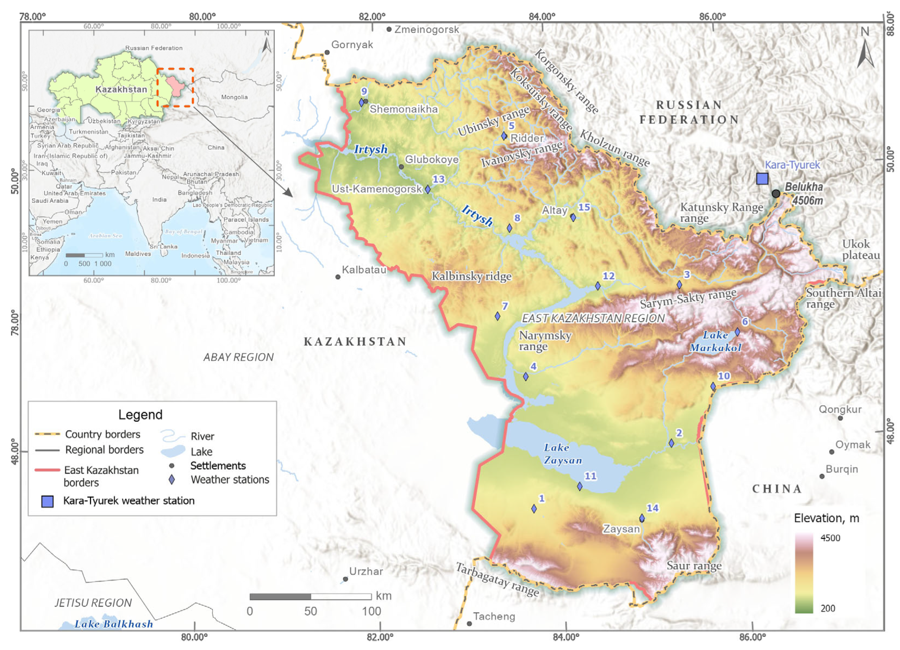
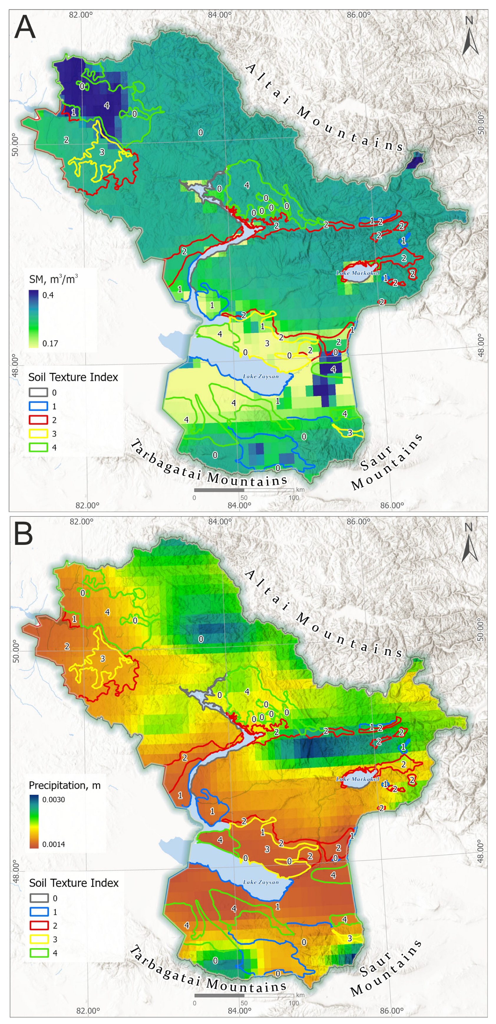
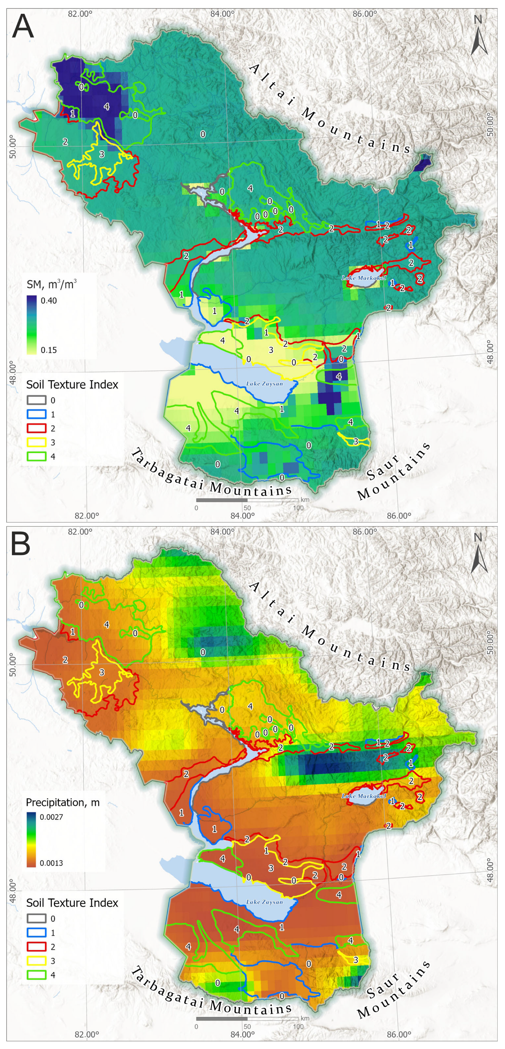
2.1. Study Area
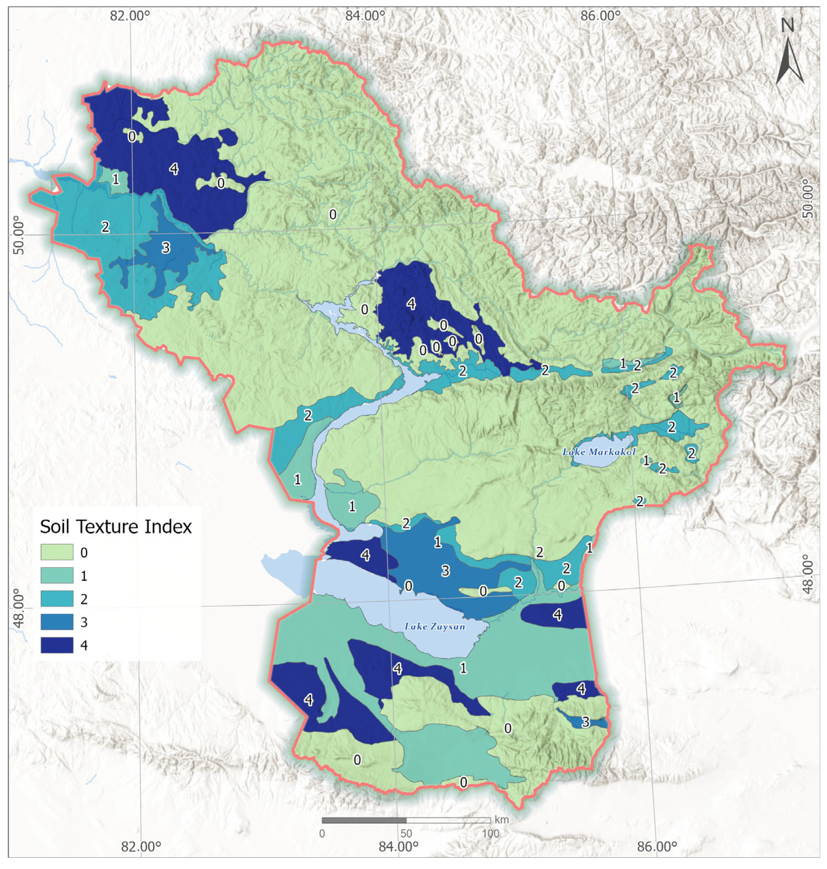
2.2. Data
- (1)
- Very light soils: sand;
- (2)
- Light soils: loamy sand;
- (3)
- Medium soils: sandy loam;
- (4)
- Heavy soils: loam + silt loam + sandy clay loam.
2.3. Methods
- Data Preparation and Filtering:
- Data for each year and soil texture class were loaded from CSV files;
- Two filtering strategies were applied: no filtering (using the entire dataset) and seasonal filtering (limiting the analysis to high-precipitation months, 6–9, and excluding days with near-zero precipitation, ≤0.001).
- Regression Analysis:
- Data for each year and soil texture class were loaded from CSV files;
- Statsmodels was used for regression analysis;
- SciPy was used for statistical testing (e.g., Shapiro–Wilk test);
- Matplotlib 3.10.0 and Seaborn v0.1 were used for data visualization.
- Software Tools:The analysis was conducted using Python (version 3.13) with the following libraries:
- Pandas for data manipulation;
- Statsmodels for regression analysis;
- SciPy for statistical testing (e.g., Shapiro–Wilk test);
- Matplotlib and Seaborn for data visualization.
- We used a simple linear regression model to relate root zone soil moisture to lagged daily precipitation: moisture_0_28cm = α + β × precipitation (lag n), where n = 0–5 days, depending on the lag configuration. We applied ordinary least squares (OLS) regression using statsmodels, assessing the significance (p < 0.05) of intercept (α) and slope (β), with residuals tested for normality using the Shapiro–Wilk test.
3. Results and Discussion
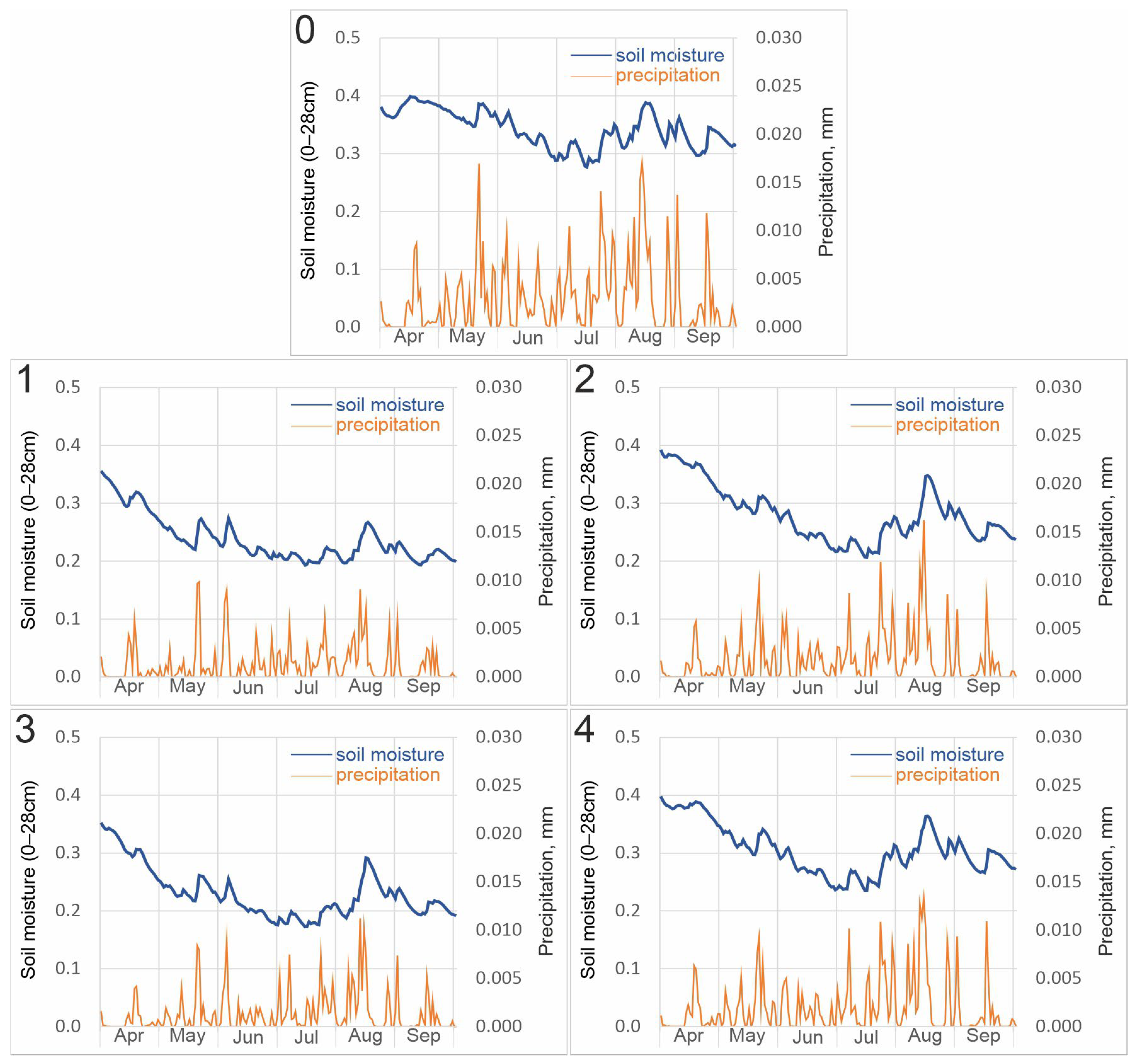
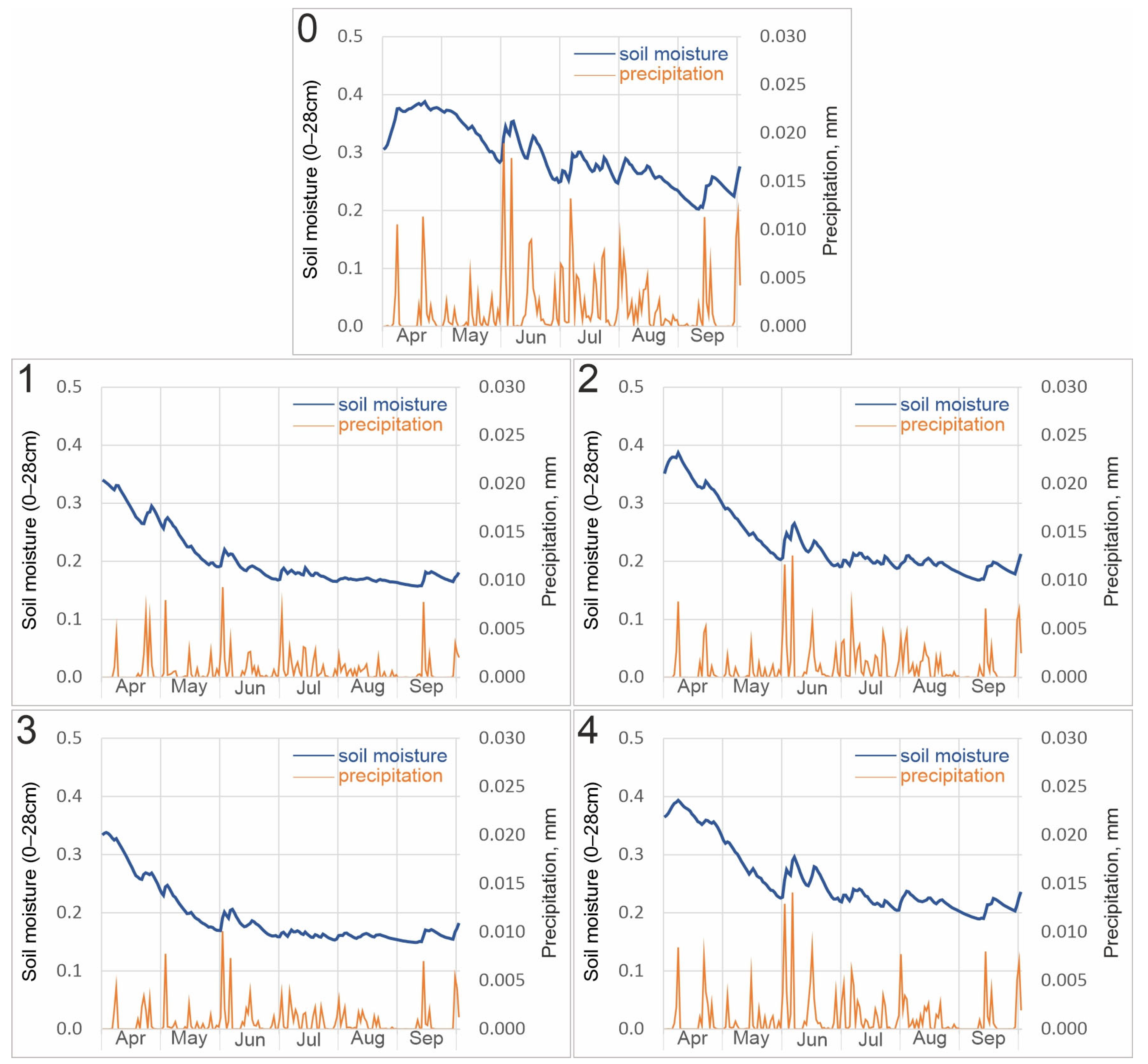
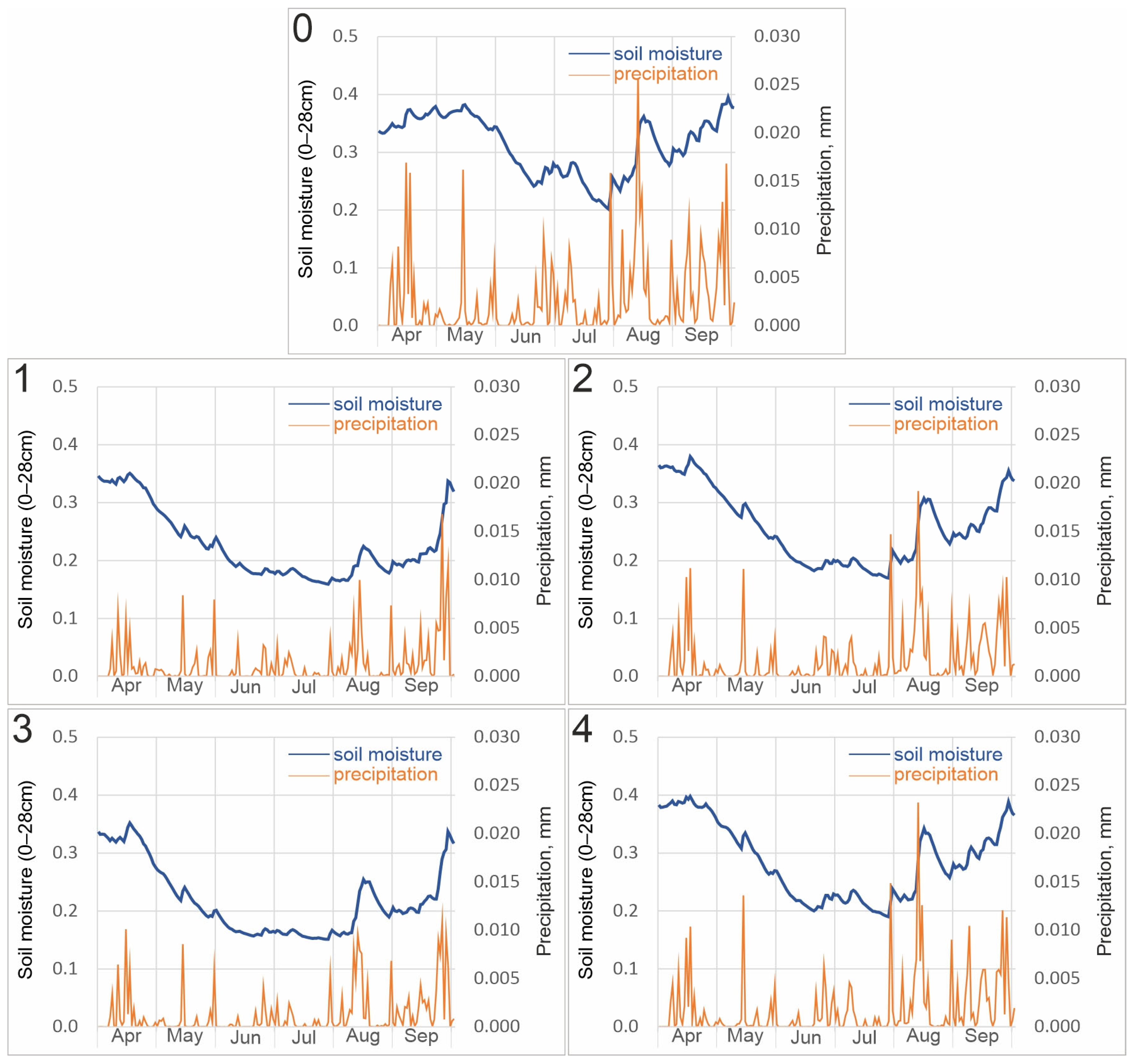
3.1. Seasonal and Interannual SM Fluctuations
3.2. The Relationship Between Soil Moisture Variability and Precipitation
4. Conclusions
Author Contributions
Funding
Data Availability Statement
Conflicts of Interest
References
- Fan, D.; Zhao, T.; Jiang, X.; García-García, A.; Schmidt, T.; Samaniego, L.; Attinger, S.; Wu, H.; Jiang, Y.; Shi, J.; et al. A Sentinel-1 SAR-Based Global 1-km Resolution Soil Moisture Data Product: Algorithm and Preliminary Assessment. Remote Sens. Environ. 2025, 318, 114579. [Google Scholar] [CrossRef]
- Bojinski, S.; Verstraete, M.; Peterson, T.C.; Richter, C.; Simmons, A.; Zemp, M. The Concept of Essential Climate Variables in Support of Climate Research, Applications, and Policy. Bull. Am. Meteorol. Soc. 2014, 95, 1431–1443. [Google Scholar] [CrossRef]
- Hollmann, R.; Merchant, C.J.; Saunders, R.; Downy, C.; Buchwitz, M.; Cazenave, A.; Chuvieco, E.; Defourny, P.; de Leeuw, G.; Forsberg, R.; et al. The ESA Climate Change Initiative: Satellite Data Records for Essential Climate Variables. Bull. Am. Meteorol. Soc. 2013, 94, 1541–1552. [Google Scholar] [CrossRef]
- Brocca, L.; Ciabatta, L.; Massari, C.; Camici, S.; Tarpanelli, A. Soil Moisture for Hydrological Applications: Open Questions and New Opportunities. Water 2017, 9, 140. [Google Scholar] [CrossRef]
- Dobriyal, P.; Qureshi, A.; Badola, R.; Hussain, S.A. A Review of the Methods Available for Estimating Soil Moisture and Its Implications for Water Resource Management. J. Hydrol. 2012, 458–459, 110–117. [Google Scholar] [CrossRef]
- Kamalanandhini, M. Scientometric Analysis-Based Review of Drought Indices for Assessment and Monitoring of Drought. Geogr. Pannonica 2023, 27, 104–118. [Google Scholar] [CrossRef]
- Dai, A. Drought under global warming: A review. WIREs Clim. Chang. 2011, 2, 45–65. [Google Scholar] [CrossRef]
- Seneviratne, S.I.; Corti, T.; Davin, E.L.; Hirschi, M.; Jaeger, E.B.; Lehner, I.; Orlowsky, B.; Teuling, A.J. Investigating Soil Moisture–Climate Interactions in a Changing Climate: A Review. Earth Sci. Rev. 2010, 99, 125–161. [Google Scholar] [CrossRef]
- Kumar, S.; Newman, M.; Lawrence, D.M.; Lo, M.-H.; Akula, S.; Lan, C.-W.; Livneh, B.; Lombardozzi, D. The GLACE-Hydrology Experiment: Effects of Land-Atmosphere Coupling on Soil Moisture Variability and Predictability. J. Clim. 2020, 33, 6511–6529. [Google Scholar] [CrossRef]
- Grillakis, M.G.; Koutroulis, A.G.; Komma, J.; Tsanis, I.K.; Wagner, W.; Blöschl, G. Initial Soil Moisture Effects on Flash Flood Generation—A Comparison between Basins of Contrasting Hydro-Climatic Conditions. J. Hydrol. 2016, 541, 206–217. [Google Scholar] [CrossRef]
- Berghuijs, W.R.; Harrigan, S.; Molnar, P.; Slater, L.J.; Kirchner, J.W. The Relative Importance of Different Flood-Generating Mechanisms across Europe. Water Resour. Res. 2019, 55, 4582–4593. [Google Scholar] [CrossRef]
- Yang, W.; Yang, H.; Yang, D. Classifying Floods by Quantifying Driver Contributions in the Eastern Monsoon Region of China. J. Hydrol. 2020, 585, 124767. [Google Scholar] [CrossRef]
- Wang, J.; Ran, Q.; Liu, L.; Pan, H.; Ye, S. Study on the Dominant Mechanism of Extreme Flow Events in the Middle and Lower Reaches of the Yangtze River. China Rural. Water Hydropower 2022, 6, 119–124. [Google Scholar]
- Ochsner, T.E.; Cosh, M.H.; Cuenca, R.H.; Dorigo, W.A.; Draper, C.S.; Hagimoto, Y.; Kerr, Y.H.; Njoku, E.G.; Small, E.E.; Zreda, M. State of the Art in Large-Scale Soil Moisture Monitoring. Soil Sci. Soc. Am. J. 2013, 77, 1888–1919. [Google Scholar] [CrossRef]
- Bogena, H.R.; Huisman, J.A.; Güntner, A.; Hübner, C.; Kusche, J.; Jonard, F.; Vey, S.; Vereecken, H. Emerging Methods for Noninvasive Sensing of Soil Moisture Dynamics from Field to Catchment Scale: A Review. WIREs Water 2015, 2, 635–647. [Google Scholar] [CrossRef]
- Li, Q.; Zhu, Q.; Zheng, J.S.; Liao, K.H.; Yang, G.H. Soil Moisture Response to Rainfall in Forestland and Vegetable Plot in Taihu Lake Basin, China. Chin. Geogr. Sci. 2015, 25, 426–437. [Google Scholar] [CrossRef]
- Babaeian, E.; Sadeghi, M.; Jones, S.B.; Montzka, C.; Vereecken, H.; Tuller, M. Ground, Proximal, and Satellite Remote Sensing of Soil Moisture. Rev. Geophys. 2019, 57, 530–616. [Google Scholar] [CrossRef]
- Robinson, D.A.; Campbell, C.S.; Hopmans, J.W.; Hornbuckle, B.K.; Jones, S.B.; Knight, R.; Ogden, F.L.; Selker, J.S.; Wendroth, O. Soil Moisture Measurement for Ecological and Hydrological Watershed-Scale Observatories: A Review. Vadose Zone J. 2008, 7, 358–389. [Google Scholar] [CrossRef]
- Zhang, X.; Zhang, T.; Zhou, P.; Shao, Y.; Gao, S. Validation Analysis of SMAP and AMSR2 Soil Moisture Products over the United States Using Ground-Based Measurements. Remote Sens. 2017, 9, 104. [Google Scholar] [CrossRef]
- Hodges, B.; Tagert, M.; Paz, J.; Meng, Q. Assessing in-field soil moisture variability in the active root zone using granular matrix sensors. Agric. Water Manag. 2023, 282, 108268. [Google Scholar] [CrossRef]
- Chai, L.; et al. QLB-NET: A Dense Soil Moisture and Freeze–Thaw Monitoring Network in the Qinghai Lake Basin on the Qinghai–Tibetan Plateau. Bull. Am. Meteorol. Soc. 2024, 105, E584–E604. [Google Scholar] [CrossRef]
- Dorigo, W.; Himmelbauer, I.; Aberer, D.; Schremmer, L.; Petrakovic, I.; Zappa, L.; Preimesberger, W.; Xaver, A.; Annor, F.; Ardö, J.; et al. The International Soil Moisture Network: Serving Earth System Science for over a decade. Hydrol. Earth Syst. Sci. 2021, 25, 5749–5804. [Google Scholar] [CrossRef]
- Kim, S.; Zhang, R.; Pham, H.; Sharma, A. A Review of Satellite-Derived Soil Moisture and Its Usage for Flood Estimation. Remote Sens. Earth Syst. Sci. 2019, 2, 225–246. [Google Scholar] [CrossRef]
- Zhuo, L. Satellite Remote Sensing of Soil Moisture for Hydrological Applications: A Review of Issues to Be Solved. In ICT for Smart Water Systems: Measurements and Data Science; Scozzari, A., Mounce, S., Han, D., Soldovieri, F., Solomatine, D., Eds.; Springer: Cham, Switzerland, 2019; Volume 102, pp. 1–20. [Google Scholar] [CrossRef]
- Zhong, M.; Zeng, T.; Jiang, T.; Wu, H.; Chen, X.; Hong, Y. A Copula-Based Multivariate Probability Analysis for Flash Flood Risk under the Compound Effect of Soil Moisture and Rainfall. Water Resour. Manag. 2021, 35, 83–98. [Google Scholar] [CrossRef]
- Al-Yaari, A.; Wigneron, J.P.; Dorigo, W.; Colliander, A.; Pellarin, T.; Hahn, S.; Mialon, A.; Richaume, P.; Fernandez-Moran, R.; Fan, L.; et al. Assessment and Inter-comparison of Recently Developed/Reprocessed Microwave Satellite Soil Moisture Products Using ISMN Ground-Based Measurements. Remote Sens. Environ. 2019, 224, 289–303. [Google Scholar] [CrossRef]
- Chen, Y.; Feng, X.; Fu, B. An Improved Global Remote-Sensing-Based Surface Soil Moisture (RSSSM) Dataset Covering 2003–2018. Earth Syst. Sci. Data 2021, 13, 1–31. [Google Scholar] [CrossRef]
- Hao, L.; Chen, J.; Wei, Z.; Miao, L.; Zhao, T.; Peng, J. Validation of Satellite Soil Moisture Products by Sparsification of Ground Observations. IEEE J. Sel. Top. Appl. Earth Obs. Remote Sens. 2024, 17, 5970–5985. [Google Scholar] [CrossRef]
- Quast, R.; Wagner, W.; Bauer-Marschallinger, B.; Vreugdenhil, M. Soil Moisture Retrieval from Sentinel-1 Using a First-Order Radiative Transfer Model—A Case-Study over the Po-Valley. Remote Sens. Environ. 2023, 295, 113651. [Google Scholar] [CrossRef]
- Atar, M.; Shah-Hosseini, R.; Ghaffari, O. Retrieval of Soil Moisture Using Time Series of Radar and Optical Remote Sensing Data at 10 m Resolution. Environ. Sci. Proc. 2024, 29, 75. [Google Scholar] [CrossRef]
- Bulut Ünal, M.; Babak, M.; Duan, Z. Estimation of Surface Soil Moisture from Sentinel-1 Synthetic Aperture Radar Imagery Using Machine Learning Method. Remote Sens. Appl. Soc. Environ. 2024, 36, 101369. [Google Scholar] [CrossRef]
- Aili, Y.; Nurmemet, I.; Li, S.; Lv, X.; Yu, X.; Aihaiti, A.; Qin, Y. Retrieval of Soil Moisture in the Yutian Oasis, Northwest China by 3D Feature Space Based on Optical and Radar Remote Sensing Data. Land 2025, 14, 627. [Google Scholar] [CrossRef]
- Rodell, M.; Houser, P.R.; Jambor, U.; Gottschalck, J.; Mitchell, K.; Meng, C.-J.; Arsenault, K.; Cosgrove, B.; Radakovich, J.; Bosilovich, M.; et al. The Global Land Data Assimilation System. Bull. Am. Meteorol. Soc. 2004, 85, 381–394. [Google Scholar] [CrossRef]
- Dorigo, W.; Wagner, W.; Albergel, C.; Albrecht, F.; Balsamo, G.; Brocca, L.; Chung, D.; Ertl, M.; Forkel, M.; Gruber, A.; et al. ESA CCI Soil Moisture for Improved Earth System Understanding: State-of-the-Art and Future Directions. Remote Sens. Environ. 2017, 203, 185–215. [Google Scholar] [CrossRef]
- Martens, B.; Miralles, D.G.; Lievens, H.; van der Schalie, R.; de Jeu, R.A.M.; Fernández-Prieto, D.; Beck, H.E.; Dorigo, W.A.; Verhoest, N.E.C. GLEAM v3: Satellite-Based Land Evaporation and Root-Zone Soil Moisture. Geosci. Model Dev. 2017, 10, 1903–1925. [Google Scholar] [CrossRef]
- Chen, Y. An Improved Remote Sensing-Based Global Surface Soil Moisture Dataset (RSSSM, 2003–2020) [Dataset]; PANGAEA: Bremen, Germany, 2022. [Google Scholar] [CrossRef]
- Lal, P.; Singh, G.; Das, N.N.; Colliander, A.; Entekhabi, D. Assessment of ERA5-Land Volumetric Soil Water Layer Product Using In Situ and SMAP Soil Moisture Observations. IEEE Geosci. Remote Sens. Lett. 2022, 19, 1–5. [Google Scholar] [CrossRef]
- Yang, J.; Yang, Q.; Hu, F.; Shao, J.; Wang, G. A Climate-Adaptive Transfer Learning Framework for Improving Soil Moisture Estimation in the Qinghai-Tibet Plateau. J. Hydrol. 2024, 630, 130717. [Google Scholar] [CrossRef]
- Varentsova, N.A.; Kireeva, M.; Kharlamov, M.; Varentsov, M.; Frolova, N.; Povalishnikova, E.S. Spring River Runoff in the European Part of Russia: Main Factors and Their Estimation. II. Reassessment in Modern Conditions on the Example of the Don Basin Rivers. Hydrometeorol. Res. Forecast. 2022, 2, 117–146. [Google Scholar] [CrossRef]
- Fan, Y.; van den Dool, H. Climate Prediction Center Global Monthly Soil Moisture Data Set at 0.5° Resolution for 1948 to Present. J. Geophys. Res. 2004, 109, D10102. [Google Scholar] [CrossRef]
- Liu, E.; Zhu, Y.; Calvet, J.; Lü, H.; Bonan, B.; Zheng, J.; Gou, Q.; Wang, X.; Ding, Z.; Xu, H.; et al. Evaluation of Model-Derived Root-Zone Soil Moisture over the Huai River Basin. Hydrol. Earth Syst. Sci. Discuss. 2023, preprint. [Google Scholar] [CrossRef]
- Ratliff, L.F.; Ritchie, J.T.; Cassel, O.K. A Survey of Field-Measured Limits of Soil Water Availability and Related Laboratory-Measured Properties. Soil Sci. Soc. Am. J. 1983, 47, 770–775. [Google Scholar] [CrossRef]
- Hanson, B.R.; Orloff, S.; Peters, D. Monitoring Soil Moisture Helps Refine Irrigation Management. Calif. Agric. 2000, 54, 38–42. [Google Scholar] [CrossRef]
- Datta, S.; Taghvaeian, S.; Stivers, J. Understanding Soil Water Content and Thresholds for Irrigation Management; Oklahoma Cooperative Extension Service, Oklahoma State University: Stillwater, OK, USA, 2017; Available online: https://extension.okstate.edu/fact-sheets/understanding-soil-water-content-and-thresholds-for-irrigation-management.html (accessed on 5 March 2025).
- Abdallah, A.M.; Jat, H.S.; Choudhary, M.; Abdelaty, E.F.; Sharma, P.C.; Jat, M.L. Conservation Agriculture Effects on Soil Water Holding Capacity and Water-Saving Varied with Management Practices and Agroecological Conditions: A Review. Agronomy 2021, 11, 1681. [Google Scholar] [CrossRef]
- Saxton, K.E.; Rawls, W.J. Soil Water Characteristic Estimates by Texture and Organic Matter for Hydrologic Solutions. Soil Sci. Soc. Am. J. 2006, 70, 1569–1578. [Google Scholar] [CrossRef]
- Ferguson, B.K. Landscape Hydrology, a Component of Landscape Ecology. J. Environ. Syst. 1991, 21, 193–205. [Google Scholar] [CrossRef]
- Chisola, M.N.; Van der Laan, M.; Bristow, K.L. A Landscape Hydrology Approach to Inform Sustainable Water Resource Management under a Changing Environment: A Case Study for the Kaleya River Catchment, Zambia. J. Hydrol. Reg. Stud. 2020, 32, 100762. [Google Scholar] [CrossRef]
- United States Department of Agriculture. Soil Mechanics Level 1 Module 3 USDA Soil Textural Classification Study Guide; USDA Soil Conservation Service: Washington, DC, USA, 1987. [Google Scholar]
- Richer-de Forges, A.C.; Arrouays, D.; Chen, S.; Dobarco, M.R.; Libohova, Z.; Roudier, P.; Minasny, B.; Bourennane, H. Hand-Feel Soil Texture and Particle-Size Distribution in Central France: Relationships and Implications. Catena 2022, 213, 106155. [Google Scholar] [CrossRef]
- Yang, H.; Yoo, H.; Lim, H.; Kim, J.; Choi, H.T. Impacts of Soil Properties, Topography, and Environmental Features on Soil Water Holding Capacities (SWHCs) and Their Interrelationships. Land 2021, 10, 1290. [Google Scholar] [CrossRef]
- Gomez-Plaza, A.; Alvarez-Rogel, J.; Albaladejo, J.; Castillo, V.M. Spatial Patterns and Temporal Stability of Soil Moisture across a Range of Scales in a Semi-Arid Environment. Hydrol. Process. 2000, 14, 1261–1277. [Google Scholar] [CrossRef]
- Venkatesh, B.; Lakshman, N.; Purandara, B.K.; Reddy, V.B. Analysis of Observed Soil Moisture Patterns under Different Land Covers in Western Ghats, India. J. Hydrol. 2011, 397, 281–294. [Google Scholar] [CrossRef]
- Sun, F.; Lü, Y.; Wang, J.; Hua, J.; Fu, B. Soil Moisture Dynamics of Typical Ecosystems in Response to Precipitation: A Monitoring-Based Analysis of Hydrological Service in the Qilian Mountains. Catena 2015, 129, 63–75. [Google Scholar] [CrossRef]
- Baumann, P.; Lee, J.; Behrens, T.; Biswas, A.; Six, J.; McLachlan, G.; Viscarra Rossel, R.A. Modelling Soil Water Retention and Water-Holding Capacity with Visible–Near-Infrared Spectra and Machine Learning. Eur. J. Soil Sci. 2022, 73, e13220. [Google Scholar] [CrossRef]
- Zhang, Y.; Wang, K.; Wang, J.; Kong, B.; Li, Y.; Shen, Y. Changes in Soil Water Holding Capacity and Water Availability Following Vegetation Restoration on the Chinese Loess Plateau. Sci. Rep. 2021, 11, 9692. [Google Scholar] [CrossRef]
- Liu, Y.; Guo, Y.; Long, L.; Lei, S. Soil Water Behavior of Sandy Soils under Semiarid Conditions in the Shendong Mining Area (China). Water 2022, 14, 2159. [Google Scholar] [CrossRef]
- Bekhovykh, Y.; Bekhovykh, L.; Lyoevin, A.; Sizov, E. Changes in Maximum Water Holding Capacity of Chernozem Soil Caused by Soil Compaction. E3S Web Conf. 2021, 262, 03003. [Google Scholar] [CrossRef]
- Bondarovich, A.A.; Mordvin, E.Y.; Pochyomin, N.M.; Lagutin, A.A. Reconstruction of Root Zone Soil Moisture According to the Data from Passive Microwave Radiometer and Machine Learning in the Arid Steppe Region of Southern Western Siberia. Acta Biol. Sibir. 2023, 9, 805–829. [Google Scholar] [CrossRef]
- Dubenok, N.N.; Novikov, A.E.; Poddubsky, A.A.; Chamurliev, G.O.; Shumakova, K.B.; Zbukarev, R.V. Water-Physical Properties of Chestnut Soils Depending on Different Tillage Practices and Irrigation Regimes. RUDN J. Agron. Anim. Ind. 2023, 18, 45–58. [Google Scholar] [CrossRef]
- Western, A.W.; Blöschl, G. On the Spatial Scaling of Soil Moisture. J. Hydrol. 1999, 217, 203–224. [Google Scholar] [CrossRef]
- Hupet, F.; Vanclooster, M. Intraseasonal Dynamics of Soil Moisture Variability within a Small Agricultural Maize Cropped Field. J. Hydrol. 2002, 261, 86–101. [Google Scholar] [CrossRef]
- Bosch, D.D.; Lakshmi, V.; Jackson, T.J.; Choi, M.; Jacobs, J.M. Large Scale Measurements of Soil Moisture for Validation of Remotely Sensed Data: Georgia Soil Moisture Experiment of 2003. J. Hydrol. 2006, 323, 120–137. [Google Scholar] [CrossRef]
- Bell, K.R.; Blanchard, B.J.; Schugge, T.J.; Witczak, M.W. Analysis of Surface Moisture Variations within Large Field Sites. Water Resour. Res. 1980, 16, 796–810. [Google Scholar] [CrossRef]
- Brocca, L.; Melone, F.; Moramarco, T.; Wagner, W. A new method for rainfall estimation through soil moistureobservations. Geophys. Res. Lett. 2013, 40, 853–858. [Google Scholar] [CrossRef]
- Brocca, L.; Ciabatta, L.; Massari, C.; Moramarco, T.; Hahn, S.; Hasenauer, S.; Kidd, R.; Dorigo, W.; Wagner, W.; Levizzani, V. Soil as a natural rain gauge: Estimating global rainfall from satellite soil moisture data. J. Geophys. Res. 2014, 119, 5128–5141. [Google Scholar] [CrossRef]
- Ciabatta, L.; Brocca, L.; Massari, C.; Moramarco, T.; Gabellani, S.; Puca, S.; Wagner, W. Rainfall-runoffmodelling by using SM2RAIN-derived and state-of-the-art satellite rainfall products over Italy. Int. J. Appl. Earth Obs. Geoinf. 2016, 48, 163–173. [Google Scholar]
- Alvarez-Garreton, C.; Ryu, D.; Western, A.W.; Crow, W.T.; Su, C.-H.; Robertson, D.R. Dual assimilation ofsatellite soil moisture to improve streamflow prediction in data-scarce catchments. Water Resour. Res. 2016, 52, 5357–5375. [Google Scholar] [CrossRef]
- Thieming, V.; Rojas, R.; Zambrano-Bigiarini, M.; De Roo, A. Hydrological evaluation of satellite-based rainfall estimates over the Volta and Baro-Akobo Basin. J. Hydrol. 2013, 499, 324–338. [Google Scholar] [CrossRef]
- Addor, N.; Seibert, J. Bias correction for hydrological impact studies—Beyond the daily perspective. Hydrol. Process. 2014, 28, 4823–4828. [Google Scholar] [CrossRef]
- Chupakhin, V. Physical Geography of Kazakhstan; Mektep Press: Almaty, Kazakhstan, 1968; p. 260. [Google Scholar]
- Veselova, L. Morphostructure of the South-Eastern Kazakhstan Mountains. In Geography of Desertic and Mountain Region of Kazakhstan; Nauka: Moskva–Leningrad, Russia, 1970; pp. 38–48. [Google Scholar]
- Novikov, I.S. Morphotectonics of Altai. Geomorfologiya 2003, 3, 10–25. [Google Scholar] [CrossRef]
- Deviatkin, E.V. The Cainozoic of the Inner Asia; Nauka: Moskva, Russia, 1981; 196p. [Google Scholar]
- Dyachkov, B.A.; Mayorova, N.P.; Chernenko, Z.I. History of East Kazakhstan Geological Structures Development in the Hercynian, Cimmerian and Alpine Cycles of Tectonic Genesis, Part II. In Proceedings of the Ust-Kamenogorsk Kazakh Geographical Society; Serikbaev, D., Ed.; East Kazakhstan State Technical University Press: Ust-Kamenogorsk, Kazakhstan, 2014; pp. 42–48. [Google Scholar]
- Chlachula, J. Pleistocene Climate Change, Natural Environments and Palaeolithic Peopling of East Kazakhstan. Quat. Int. 2010, 220, 64–87. [Google Scholar] [CrossRef]
- Yegorina, A. The Climate of Southwest Altai; Semipalatinsk University Press: Semey, Kazakhstan, 2015; p. 315. [Google Scholar]
- Kottek, M.; Grieser, J.; Beck, C.; Rudolf, B.; Rubel, F. World Map of the Köppen–Geiger Climate Classification Updated. Meteorol. Z. 2006, 15, 259–263. [Google Scholar] [CrossRef]
- World Bank. Kazakhstan. Climate Change Overview Country Summary. Climate Change Knowledge Portal. Available online: https://climateknowledgeportal.worldbank.org/country/kazakhstan (accessed on 19 March 2025).
- Weather and Climate of Kazakhstan. Weather-and-Climate.com 2025. Available online: https://weather-and-climate.com/average-monthly-Rainfall-Temperature-Sunshine-in-Kazakhstan (accessed on 19 March 2025).
- Geldiyeva, G.; Vesselova, L. Landscapes of Kazakhstan; Gylym: Alma-Ata, Kazakhstan, 1992; 176p. [Google Scholar]
- Bormann, H. Towards a Hydrologically Motivated Soil Texture Classification. Geoderma 2010, 157, 142–153. [Google Scholar] [CrossRef]
- Voronina, L.M. (Ed.) Soil Map of the Kazakh SSR; GUGK: Moscow, Russia, 1976. [Google Scholar]
- Muñoz Sabater, J. ERA5-Land hourly data from 1950 to present* [Data set]. Copernicus Climate Change Service (C3S) Climate Data Store. 2019. Available online: https://doi.org/10.24381/cds.e2161bac (accessed on 10 March 2025).
- Vasiliev, O.; Semenov, V.; Tuleubayev, Z.; Vasiliev, A.; Sarsembayeva, A.; Yesembekova, Z.; Ziyaeva, G. Loess-Like Loams as a Soil Formation Factor for Light-Gray Forest Soils in the Cheboksary Region of the Chuvash Republic. Bull. Acad. Sci. Kazakh SSR 2020, 6, 38–45. [Google Scholar] [CrossRef]
- Zheng, Y.; Coxon, G.; Woods, R.; Power, D.; Rico-Ramirez, M.A.; McJannet, D.; Rosolem, R.; Li, J.; Feng, P. Evaluation of Reanalysis Soil Moisture Products Using Cosmic-Ray Neutron Sensor Observations Across the Globe. Hydrol. Earth Syst. Sci. 2024, 28, 1999–2022. [Google Scholar] [CrossRef]
- Klang, P.S.; Khan, V.M.; Tarasova, L.L. Estimation of Volumetric Soil Moisture from ERA5 Reanalysis According to the Station Observations of Moisture Reserves in the Regions of the Russian Federation. Hydrometeorol. Res. Forecast. 2024, 4, 146–162. [Google Scholar] [CrossRef]
- Trenberth, K.E.; Asrar, G.R. Challenges and opportunities in water cycle research: WCRP contributions. Surv. Geophys. 2014, 35, 515–532. [Google Scholar] [CrossRef]


| Soil Texture Class | SM Fluctuations | |||||||||
|---|---|---|---|---|---|---|---|---|---|---|
| 2013—Extremely Humid | 2022—Extremely Dry | 2023—Mean | ||||||||
| Max | Min | Mean | Max | Min | Mean | Max | Min | Mean | ||
| 0 | 0.40 | 0.28 | 0.34 | 0.39 | 0.20 | 0.31 | 0.39 | 0.20 | 0.30 | |
| 1 | 0.36 | 0.19 | 0.24 | 0.35 | 0.16 | 0.23 | 0.34 | 0.16 | 0.20 | |
| 2 | 0.39 | 0.21 | 0.28 | 0.38 | 0.17 | 0.26 | 0.39 | 0.17 | 0.23 | |
| 3 | 0.35 | 0.17 | 0.23 | 0.35 | 0.15 | 0.22 | 0.34 | 0.15 | 0.19 | |
| 4 | 0.40 | 0.24 | 0.31 | 0.40 | 0.19 | 0.29 | 0.39 | 0.19 | 0.26 | |
| Year | Texture Class | Optimal Lag | α | β | Pearson Corr. | n_Samples |
|---|---|---|---|---|---|---|
| 2013 | 0 | 1 | 0.31 | 4.25 | 0.60 | 77 |
| 2013 | 1 | 1 | 0.20 | 6.02 | 0.62 | 57 |
| 2013 | 2 | 1 | 0.23 | 6.07 | 0.55 | 63 |
| 2013 | 3 | 1 | 0.19 | 6.05 | 0.56 | 50 |
| 2013 | 4 | 1 | 0.26 | 5.97 | 0.62 | 58 |
| 2022 | 0 | 3 | 0.26 | 3.47 | 0.49 | 51 |
| 2022 | 1 | 2 | 0.17 | 2.60 | 0.54 | 27 |
| 2022 | 2 | 3 | 0.19 | 2.91 | 0.48 | 41 |
| 2022 | 3 | 2 | 0.16 | 3.40 | 0.72 | 31 |
| 2022 | 4 | 3 | 0.22 | 3.39 | 0.55 | 35 |
| 2023 | 0 | 1 | 0.27 | 4.59 | 0.44 | 63 |
| 2023 | 1 | 3 | 0.18 | 8.01 | 0.62 | 34 |
| 2023 | 2 | 3 | 0.23 | 5.36 | 0.37 | 52 |
| 2023 | 3 | 1 | 0.16 | 10.82 | 0.73 | 37 |
| 2023 | 4 | 1 | 0.26 | 4.42 | 0.35 | 46 |
Disclaimer/Publisher’s Note: The statements, opinions and data contained in all publications are solely those of the individual author(s) and contributor(s) and not of MDPI and/or the editor(s). MDPI and/or the editor(s) disclaim responsibility for any injury to people or property resulting from any ideas, methods, instructions or products referred to in the content. |
© 2025 by the authors. Licensee MDPI, Basel, Switzerland. This article is an open access article distributed under the terms and conditions of the Creative Commons Attribution (CC BY) license (https://creativecommons.org/licenses/by/4.0/).
Share and Cite
Chernykh, D.; Biryukov, R.; Bondarovich, A.; Lubenets, L.; Pavlenko, A.; Rakhymbek, K.; Revenko, D.; Zhantassova, Z. Spatiotemporal Analysis of Soil Moisture Variability and Precipitation Response Across Soil Texture Classes in East Kazakhstan. Land 2025, 14, 1136. https://doi.org/10.3390/land14061136
Chernykh D, Biryukov R, Bondarovich A, Lubenets L, Pavlenko A, Rakhymbek K, Revenko D, Zhantassova Z. Spatiotemporal Analysis of Soil Moisture Variability and Precipitation Response Across Soil Texture Classes in East Kazakhstan. Land. 2025; 14(6):1136. https://doi.org/10.3390/land14061136
Chicago/Turabian StyleChernykh, Dmitry, Roman Biryukov, Andrey Bondarovich, Lilia Lubenets, Anatoly Pavlenko, Kamilla Rakhymbek, Denis Revenko, and Zheniskul Zhantassova. 2025. "Spatiotemporal Analysis of Soil Moisture Variability and Precipitation Response Across Soil Texture Classes in East Kazakhstan" Land 14, no. 6: 1136. https://doi.org/10.3390/land14061136
APA StyleChernykh, D., Biryukov, R., Bondarovich, A., Lubenets, L., Pavlenko, A., Rakhymbek, K., Revenko, D., & Zhantassova, Z. (2025). Spatiotemporal Analysis of Soil Moisture Variability and Precipitation Response Across Soil Texture Classes in East Kazakhstan. Land, 14(6), 1136. https://doi.org/10.3390/land14061136