Wavelet-Based Analysis of Subsidence Patterns and High-Risk Zone Delineation in Underground Metal Mining Areas Using SBAS-InSAR

Abstract

Underground metal mines operated using the natural caving method often result in significant surface collapses. Key parameters such as settlement magnitude, settlement rate, settlement extent, and the influence of underground mining on surface deformation warrant serious attention. However, due to the long operational timespan of mines and incomplete data from early collapse events, coupled with the inaccessibility of collapse zones for field measurements, it is challenging to obtain accurate displacement data, thereby posing significant difficulties for follow-up research. This study employs small baseline subset InSAR (SBAS-InSAR) technology to retrieve time series data on early-stage surface displacement and deformation rates in collapse areas, thereby compensating for the lack of historical data and eliminating the safety risks associated with on-site measurements. The 5th percentile of settlement rates across all monitoring points is used to define the severe settlement threshold, determined to be −42.1 mm/year. Continuous wavelet transform (CWT) is applied to calculate the time-series power spectrum, allowing the analysis of long-term stable and periodic settlement patterns in the collapse area. The instantaneous change rate at each point in the study area is identified. Using the 97th percentile of change rates in the time series, the number of severe change events at each point is determined. High-incidence zones of sudden surface deformation are visualized through QGIS 3.16 heat map clustering. The high-risk collapse area, identified by integrating both long-term stable settlement and sudden surface deformation patterns, accounts for multiple deformation modes. This provides robust technical support for the management of mine collapse zones and offers important theoretical guidance.

1. Introduction

The natural caving method is widely applied in the extraction of inclined and steeply inclined, thick, large-scale metal deposits due to its advantages of high production capacity, efficiency, and low cost [1]. However, as mining depth and extent increase, varying degrees of surface subsidence and collapse may occur, potentially leading to anthropogenic ecological degradation [2].

To improve risk management in the subsidence area and better understand the extent of its impact and the severity of surface damage, it is essential to conduct a comprehensive analysis of settlement displacement and subsidence rate. Ground surface subsidence is often influenced by the mechanical properties of geological bodies, tectonic fault movements, groundwater variations, and rainfall. Underground mining activities alter the mechanical state of geological bodies, damage original geological structures and hydrogeological conditions, and consequently induce varying degrees of ground subsidence [3,4]. However, due to the mechanical characteristics of rock masses (e.g., anisotropy and elasto-plasticity), surface collapse is a complex nonlinear phenomenon, exhibiting patterns such as continuous, periodic, and sudden subsidence. Temporally, subsidence exhibits characteristics of continuity, hysteresis, and abrupt changes [5,6]. To effectively characterize subsidence patterns in the collapse area, the temporal and displacement information embedded in long-term displacement sequences is utilized. Mathematical transformations (e.g., Fourier transform, wavelet transform) are applied to extract frequency and energy information [7,8]. By analyzing multiple time scales, distinct subsidence patterns can be identified.

First, it is essential to acquire surface subsidence data. Traditionally, this is achieved through direct ground-based measurements [9]. However, many collapse zones are inaccessible, making traditional field measurements difficult or unsafe. Currently, surface collapse in goaf areas is primarily monitored using UAV-based scanning [10] and Interferometric Synthetic Aperture Radar (InSAR) displacement techniques [11,12], which can accurately capture the extent, magnitude, and rate of settlement in complex terrain. Among conventional techniques, Differential Interferometric Synthetic Aperture Radar (D-InSAR) [13,14,15] can accurately detect minor surface elevation changes and displacements, achieving millimeter-level accuracy under ideal conditions. It is particularly effective for monitoring surface deformations caused by earthquakes, volcanic activity, and similar geohazards. However, it requires precisely co-registered radar image pairs and an appropriate temporal acquisition interval. Otherwise, it becomes challenging to eliminate terrain-related phase noise, resulting in poor-quality interferograms. Persistent Scatterer InSAR (PS-InSAR) [16,17,18] effectively addresses spatiotemporal decorrelation by identifying long-term stable scatterers (e.g., buildings, utility poles) as monitoring targets. It provides reliable measurements even in vegetation-covered or urban areas, making it suitable for complex surface conditions. However, it only captures displacement at discrete scatterer locations and cannot characterize deformation in areas lacking such points. As a result, it often needs to be combined with other techniques to obtain a complete deformation field. Small Baseline Subset InSAR (SBAS-InSAR) [19,20,21] is well-suited for long-term time-series analysis and can handle image datasets spanning extended periods. By analyzing multiple small-baseline interferometric pairs, it more accurately captures long-term trends and seasonal variations in surface deformation. It is especially advantageous for monitoring slow, continuous processes such as urban ground subsidence. Nonetheless, SBAS-InSAR requires complex algorithms and substantial computational resources. The processing workflow is more cumbersome and time-consuming, placing higher demands on hardware capabilities.

Surface deformation in mining subsidence areas is typically influenced by multiple factors. Variations in the depth, area, and geometry of underground goafs, along with geological activity and periodic rainfall, lead to different responses in surface deformation rates [22]. The displacement time series often requires further analysis, depending on the research objectives. Statistical methods: The autoregressive integrated moving average (ARIMA) model [23] is suitable for both stationary and non-stationary time series. It effectively captures trends and seasonality and offers strong interpretability. However, it assumes data stationarity and struggles with complex nonlinear patterns, making it more suitable for short-term trend forecasting. Seasonal and trend decomposition using loess (STL) decomposition [24] intuitively separates trend, seasonal, and residual components, making it suitable for deformation analysis with clear periodicity (e.g., seasonal freeze–thaw subsidence). Machine learning methods: Support Vector Regression (SVR) [25] handles small sample sizes and nonlinear problems well, but kernel selection is highly dependent on subjective expertise. Random Forest (RF) [26] supports high-dimensional feature analysis and multi-source data fusion with strong resistance to overfitting. However, it lacks the ability to capture temporal dependencies, making it more suitable for multi-factor correlation analysis (e.g., groundwater level vs. displacement). Deep learning methods: The long short-term memory (LSTM) network [27], a type of recurrent neural network, is specifically designed for sequence data and can capture long-term dependencies. However, it has high computational cost and complex hyperparameter tuning, making it more suitable for multi-sensor fusion (e.g., GNSS and inclinometer data). The Transformer model [28] captures global dependencies via self-attention mechanisms and is suitable for ultra-long sequence modeling. However, it requires large-scale datasets (>100,000 samples) and significant computational resources.

The degree of surface subsidence and the extent of its expansion in the study area directly influence the future mining plans of the mine. Understanding the spatial extent and temporal duration of mining-induced surface subsidence is crucial. Yuan et al. [29] utilized the SBAS-InSAR method combined with a slope landslide analysis to delineate the boundaries of mining-induced surface subsidence. Liu et al. [27] performed a predictive analysis of mining-induced surface subsidence using SBAS-InSAR data combined with the AT-LSTM algorithm. Chen et al. [30] predicted subsidence areas by integrating SBAS-InSAR data, UAV measurements, and the GA-BP neural network model. Those studies primarily relied on long-term displacement data, combining different algorithms to predict the subsidence state for risk management purposes. However, they did not account for the multiple temporal patterns of geological rock mass subsidence, particularly neglecting short-term abrupt subsidence in delineating the subsidence extent.

In the context of surface subsidence caused by underground metal mining, obtaining multi-year surface deformation data quickly, safely, and accurately is a key challenge. Small baseline subset InSAR (SBAS-InSAR) [21,31] offers sufficient measurement accuracy while eliminating the safety risks associated with ground-based measurements. Additionally, it provides a long-term record of surface deformation, enabling further temporal analysis. SBAS-InSAR data provides spatiotemporally continuous but non-stationary deformation signals, including gradual millimeter-level subsidence and sudden centimeter-level collapses. Given the limited dataset size, a wavelet analysis [32]—with its excellent time-frequency localization and multi-scale decomposition capabilities—can effectively detect abrupt changes (e.g., collapse precursors) and separate long-term trends from periodic components through low- and high-frequency analysis.

This study addresses both long-term trends and short-term fluctuations in subsidence behavior within collapse areas. Time-series surface deformation data are obtained using SBAS-InSAR, and the annual average subsidence rate threshold is calculated to identify severely subsided zones induced by mining activities. A wavelet analysis is applied to detect abrupt change points and to determine the threshold of instantaneous deformation velocity for identifying short-term sudden collapses. By integrating both long-term and instantaneous subsidence rates, high-risk areas can be delineated with greater accuracy.

2. Study Area and Engineering Geological Setting

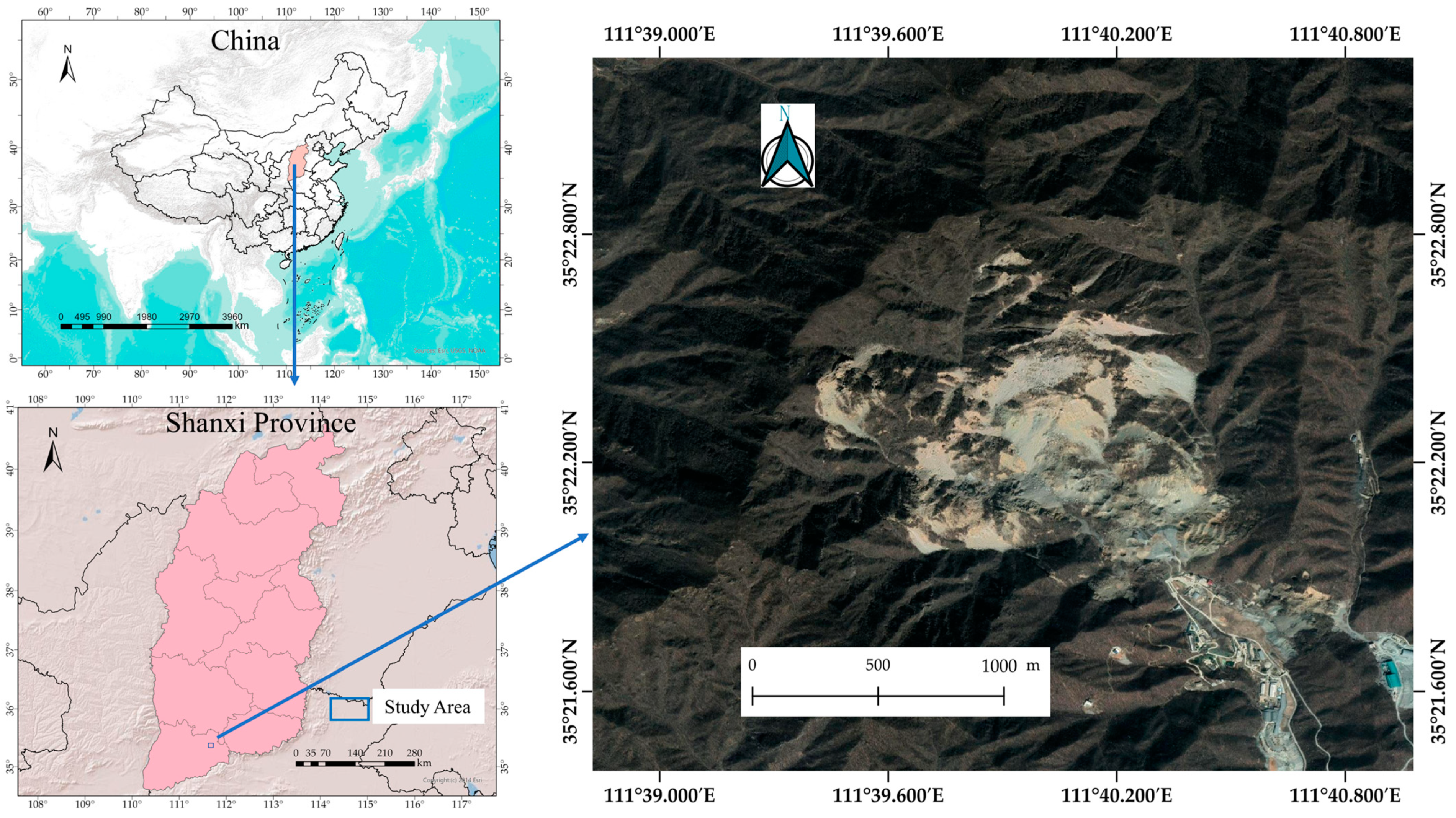
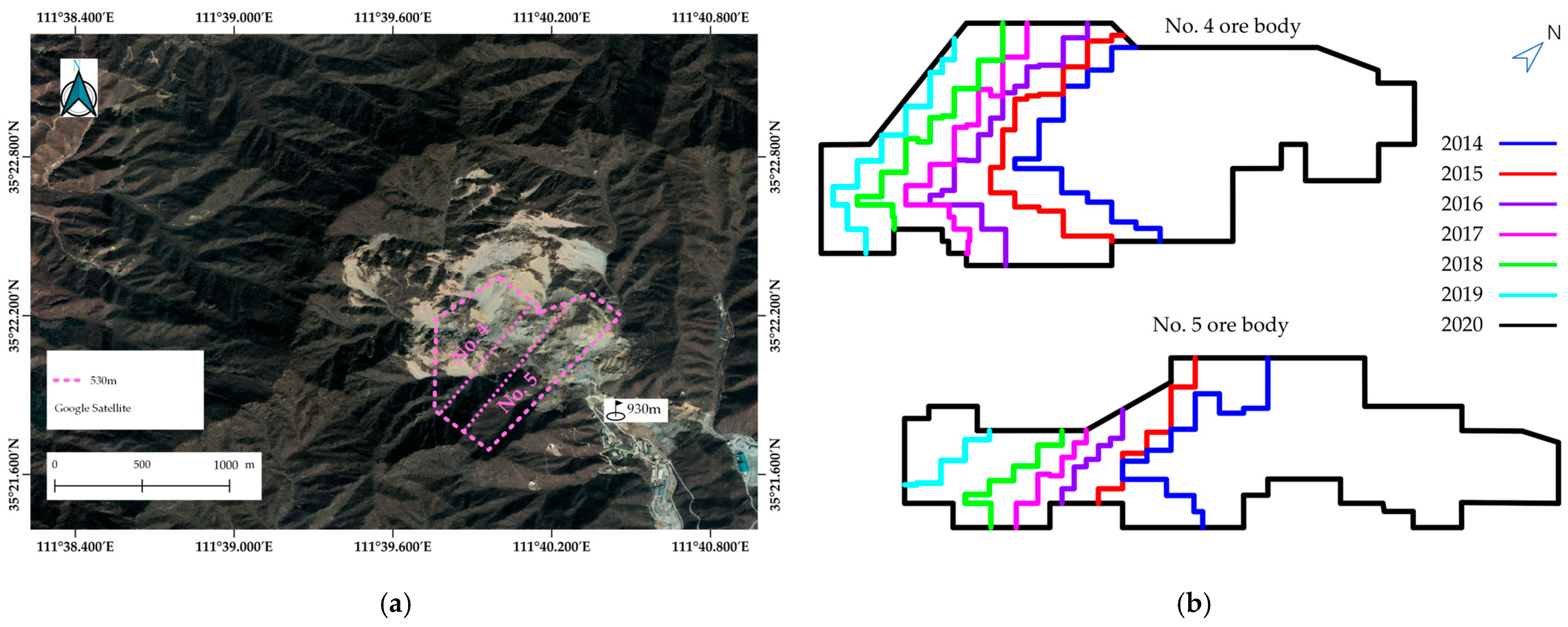
2.1. Area of Study

The Tongkuangyu Mine, operated by Northern Copper Industry Co., Ltd., is located approximately 4 km north of Yuanqu County, Shanxi Province. The mining area is enclosed by mountains on all sides. The geographical coordinates of the site range from 111°39′30″ to 111°41′13″ E longitude and 35°19′57″ to 35°22′31″ N latitude. The highest above-sea-level (ASL) elevation within the mining area is 1699.2 m. The erosion datum plane is at an elevation of 685 m, with a relative topographic relief ranging from 300 to 600 m. The total area of the mining site is approximately 5.1 square km.

The Tongkuangyu Copper Mine has employed the caving mining method continuously since its initial development. Currently, surface collapse has occurred above the ore body. The collapse zone is situated northwest of the 930 m industrial platform. The boundary of the collapse zone lies approximately 150 m from Auxiliary Shaft No. 1. The extent of the study area is illustrated in Figure 1. Satellite imagery used in this study was obtained from Google Earth Pro 7.3.6.

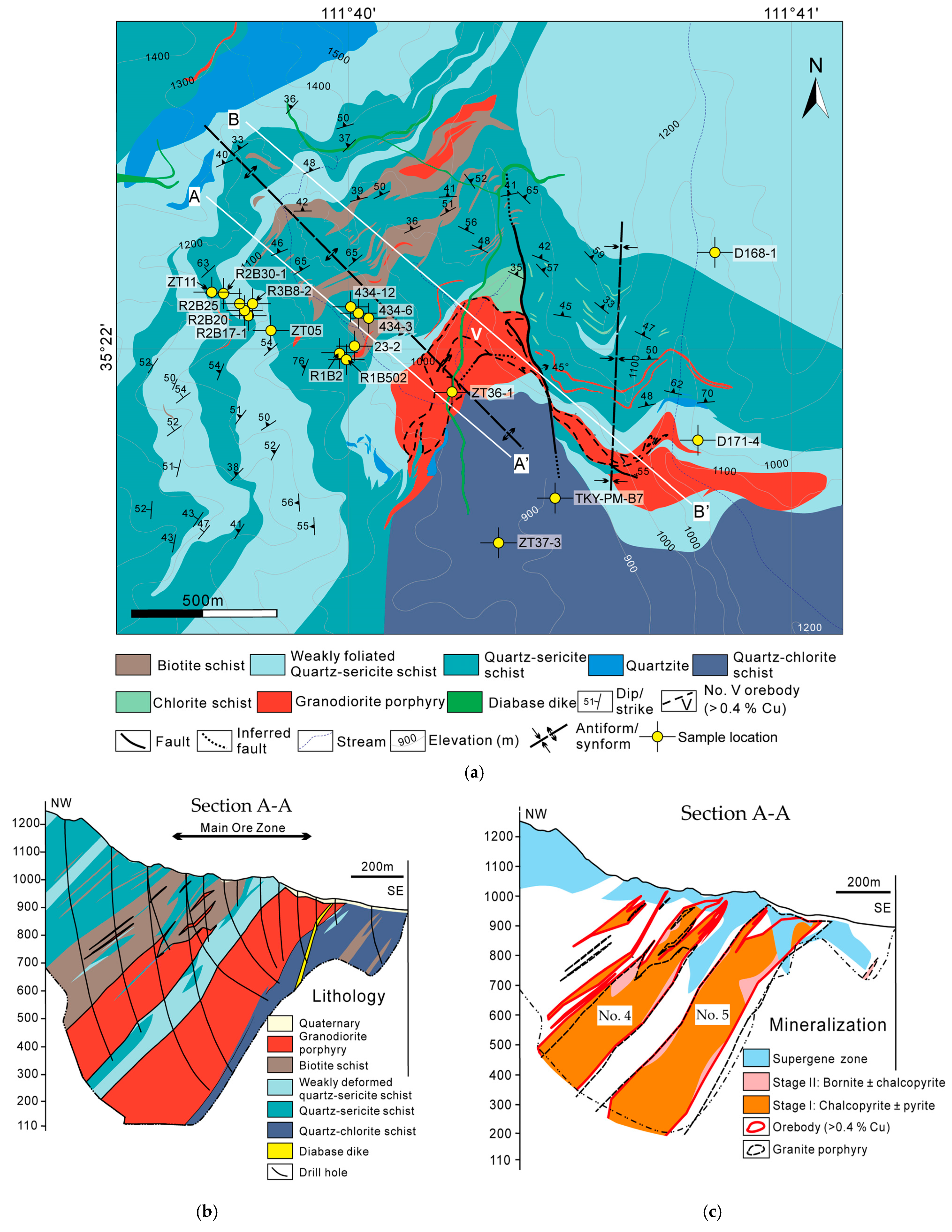
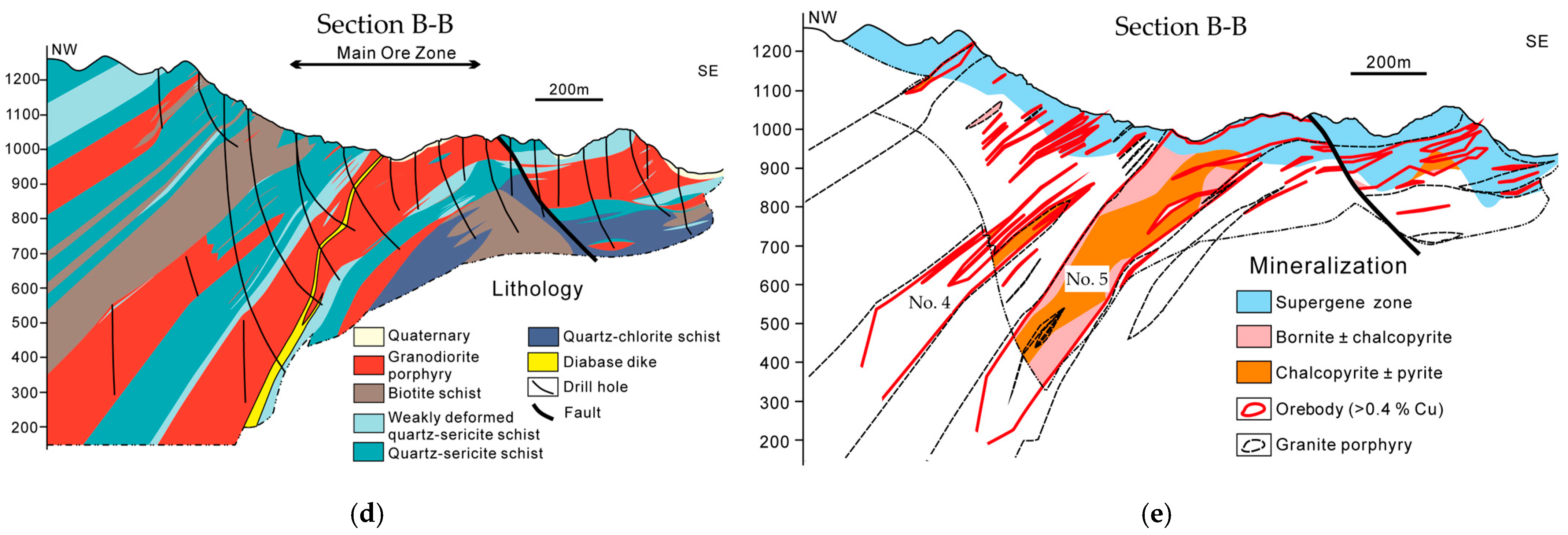
2.2. Engineering Geological Setting

The Tongkuangyu deposit is composed of two main ore bodies, designated as No. 4 and No. 5. These ore bodies are spatially parallel, with a relatively consistent spacing ranging from 110 to 130 m. In the plan view, each ore body exhibits a large lenticular shape, while along the dip direction, it resembles a plate. The ore bodies show a westward branching extension and are primarily hosted within altered potassium-rich mafic volcanic rocks. Their attitude is generally consistent with that of the surrounding strata, dipping northwest at an angle of 40° to 60°.

The primary ore-bearing lithologies in the mining area are altered quartz crystal tuff (Ma) and altered quartz porphyry (Mb), while the main wall rock is sericite quartzite (Sq). Both the ore bodies and wall rocks exhibit stable to moderately stable geotechnical conditions. The groundwater in the mining area is primarily composed of bedrock fissure water. The geological plan view and cross-sectional profile of the mining area are presented in Figure 2 [33].

The first phase of the Tongkuangyu Mine commenced operations in 1974, with a designed production capacity of 7 million tons per year. The initial mining design targeted ore bodies located above the 690 m elevation. In 1986, the natural caving mining method was introduced, and the design capacity was expanded to 40 million tons per year. The vertical height of the stope reaches 120 m. The first mining level was the 810 m section, with production ceasing at the end of 2003. The second level, the 690 m section, began production in late April 2000 and was depleted by 2014.

The second phase of the project commenced production in 2010, targeting ore bodies above the 530 m level. It was initially designed with a production capacity of 6 million tons per year. By 2018, the actual production capacity had increased to 7.5 million tons per year. In 2021, mining operations extended to ore bodies above the 410 m level, with a production capacity of 9 million tons per year. The remaining ore reserves of the second phase are expected to sustain production until 2031. The annual advancement lines of mining operations are illustrated in Figure 3.

Regional rainfall also contributes to surface subsidence. In this study, total precipitation and maximum daily precipitation from January 2016 to April 2020 in the subsidence area are analyzed as reference indicators for periodic subsidence (Figure 4). As shown in Figure 4, rainfall peaked in June and July of 2016. From April to October in both 2017 and 2018, although overall rainfall was not extreme, monthly precipitation remained around 100 mm. In 2019, rainfall events were more frequent from April to June and again from August to October. However, rainfall in July 2019 was relatively low compared to the same period in previous years.

3. Methods

This study employs SBAS-InSAR technology to process Sentinel-1A imagery within the SARscape 5.6.2 software environments. The main processing steps include connection graph generation, interferometric processing, two-stage inversion, and geocoding. After deriving the average displacement rate and time series using SBAS-InSAR technology, each dataset is processed independently for further analysis. For the average displacement rate, all negative velocities are extracted, and the 5th percentile is used as the threshold for annual subsidence. For the displacement time series, detrending, normalization, and smoothing are performed, followed by continuous wavelet transform to generate the wavelet power spectrum. Mutation point detection is then applied to determine the threshold of short-term deformation velocity. The number of significant deformation events is obtained through statistical analysis. Finally, QGIS 3.16 is used to visualize both the average displacement rate and the number of significant deformation events, delineating high-risk subsidence zones. The overall technical workflow is illustrated in Figure 5.

3.1. SBAS-InSAR Subsidence Monitoring

This study employs the Small Baseline Subset Interferometric Synthetic Aperture Radar (SBAS-InSAR) technique to derive cumulative displacement time series and surface subsidence rates induced by underground mining [34,35]. The SBAS-InSAR method effectively mitigates atmospheric phase delays and orbital errors, enhancing the spatiotemporal resolution of deformation monitoring [36]. Data processing is conducted using ENVI 5.6 and SARscape 5.6.2 software environments. The processing workflow includes interferogram generation, phase unwrapping, time-series analysis, and deformation rate estimation [37].

SBAS-InSAR constructs an interferogram network by selecting image pairs with short temporal and spatial baselines to minimize spatiotemporal decorrelation and atmospheric disturbances. The master image is designated as M₀, and all other images Mᵢ (i = 1, 2,…, N) are co-registered to it. Interferometric phases are then calculated between M₀ and each corresponding Mᵢ [38,39].

$${\varphi }_{\mathrm{int}}\left(x,y\right)={\varphi }_{\mathrm{topo}}\left(x,y\right)+{\varphi }_{\mathrm{disp}}\left(x,y\right)+{\varphi }_{\mathrm{atm}}\left(x,y\right)+{\varphi }_{\mathrm{noise}}\left(x,y\right)$$

(1)

Here, ϕ_int(x, y) denotes the total interferometric phase. ϕ_topo(x, y) represents the topographic phase, which is removed using a digital elevation model (DEM). ϕ_disp(x, y) corresponds to the deformation phase, which contains information on surface displacement. ϕ_atm(x, y) accounts for phase delays induced by atmospheric effects, while ϕ_noise(x, y) represents system noise. After topographic phase removal, the Least Squares Phase Unwrapping (LSP-U) method is applied to the interferometric phase to retrieve continuous surface deformation information.

A time-series analysis is performed on the unwrapped interferometric phase. The deformation time series is estimated using the Singular Value Decomposition (SVD) method, and the deformation rate V(x,y) is subsequently calculated. The corresponding expression is given as follows [40,41]:

$$V\left(x,y\right)={\displaystyle \frac{\sum _{i=1}^N{w}_i·\Delta {\varphi }_i\left(x,y\right)}{\sum _{i=1}^N{w}_i·\Delta t_i}}$$

(2)

Here, Δϕᵢ(x, y) denotes the unwrapped phase difference in the i-th interferometric pair. Δtᵢ represents the temporal interval of the corresponding interferometric pair. wᵢ is the weight factor, calculated based on the baseline length and coherence of the interferometric pair to enhance the accuracy of deformation rate estimation.

To mitigate the impact of atmospheric delays in the time series, a combination of high-pass filtering (HPF) and low-pass filtering (LPF) is applied for error correction. In addition, an elevation–deformation regression analysis is used to remove residual atmospheric artifacts [42,43]. The final deformation rate S(x,y) is calculated as follows:

$$S\left(x,y\right)={\displaystyle \frac{d{\varphi }_{\mathrm{disp}}\left(x,y\right)}{dt}}·{\displaystyle \frac{\lambda }{4\pi }}$$

(3)

Here, ${\displaystyle \frac{d{\varphi }_{\mathrm{disp}}\left(x,y\right)}{dt}}$ represents the deformation rate per unit time, and λ denotes the wavelength of the SAR sensor (e.g., 5.6 cm for Sentinel-1 data). This equation converts phase variations into actual surface displacement rates, enabling the derivation of subsidence rate distributions caused by underground mining.

The deformation rate map and cumulative displacement time series derived in this study facilitate the analysis of surface collapse processes induced by underground mining and provide essential data for subsequent collapse prediction and risk assessment.

Accuracy verification of SBAS-InSAR results can be performed using two main methods: external validation and internal error assessment. External validation requires high-precision deformation data from ground-based GPS stations or leveling surveys, which are then compared point by point with SBAS-InSAR results to calculate metrics such as root mean square error (RMSE) or the coefficient of determination (R²). This method provides direct and highly credible verification. However, the limitation lies in the sparse spatial distribution of ground stations, which makes it challenging to represent the entire study area.

In the absence of external data (e.g., GNSS or leveling), internal quality indicators from SBAS-InSAR processing must be used to assess the accuracy and reliability of results. The SBAS-InSAR workflow in SARscape generates model fitting errors (RMSE) as internal indicators of result accuracy. RMSE refers to the root mean square difference (in millimeters) between the observed displacement and the displacement predicted by the model. A low RMSE (typically a few millimeters) indicates that the observed deformation closely follows the model (e.g., a stable linear trend), reflecting high accuracy and low residual noise. In contrast, a high RMSE (tens of millimeters) suggests considerable discrepancies caused by phase noise, unwrapping errors, or complex deformation patterns that deviate from the assumed linear model. When ground truth data are unavailable, RMSE can be used to flag potentially unreliable or suspicious pixels.

Following the completion of mining activities for the ore body above 690 m at Tongkuangyu Mine in late 2014, a complete goaf was formed. The ore body above 530 m was subsequently extracted by 2020. Based on the formation timeline of the goaf, the image acquisition period for the study area was set from 15 June 2015 to 15 June 2020, with a 12-day revisit cycle, resulting in a total of 117 scenes. Sentinel-1A imagery acquired in ascending orbit mode and Single Look Complex (SLC) format was selected. The data were acquired in Interferometric Wide (IW) swath mode with VV polarization. The 30 m Shuttle Radar Topography Mission (SRTM) DEM was used as the digital elevation model.

The dataset was processed using the SBAS-InSAR module in ENVI SARscape 5.6.2 radar image processing software. A total of 117 input scenes were connected for interferometric processing. The spatial baseline threshold was set at 2%, and the temporal baseline threshold at 90 days. The redundancy degree was set to low, with “minimum normal baseline” selected as the redundancy criterion, and a maximum of eight connections per acquisition allowed. This resulted in the generation of 293 interferometric pairs. The spatio-temporal distribution and baseline connectivity of the dataset are illustrated in Figure 6. During interferometric processing, a multi-look ratio of 7:2 was applied. Goldstein filtering was employed, and phase unwrapping was conducted using the minimum cost flow algorithm with a threshold of 0.1 and a default unwrapping level of 1. For the first deformation rate inversion, the product coherence threshold was set at 0.1, consistent with the unwrapping threshold. A linear model was adopted for the displacement model, with a spatial wavelet size of 1200 m. The minimum valid interferogram ratio was set to 65%, and eight parallel unwrapping processes were utilized. The unwrapping decomposition level was set to 2, the refinement radius was 22.5 m, and the residual phase polynomial degree for refinement was 3. In the second deformation rate inversion, the product coherence threshold remained at 0.1. Atmospheric filtering parameters included a low-pass size of 1600 m and a high-pass size of 365 days. During geocoding, the height and velocity precision thresholds were both set to 100. The spatial resolution in both X and Y dimensions was set to 30 m, consistent with the DEM. The product temporal coherence threshold was set to 0.1, the residual phase polynomial degree for refinement was 1, and the mean window size was set to 3. All other parameters were retained as default.

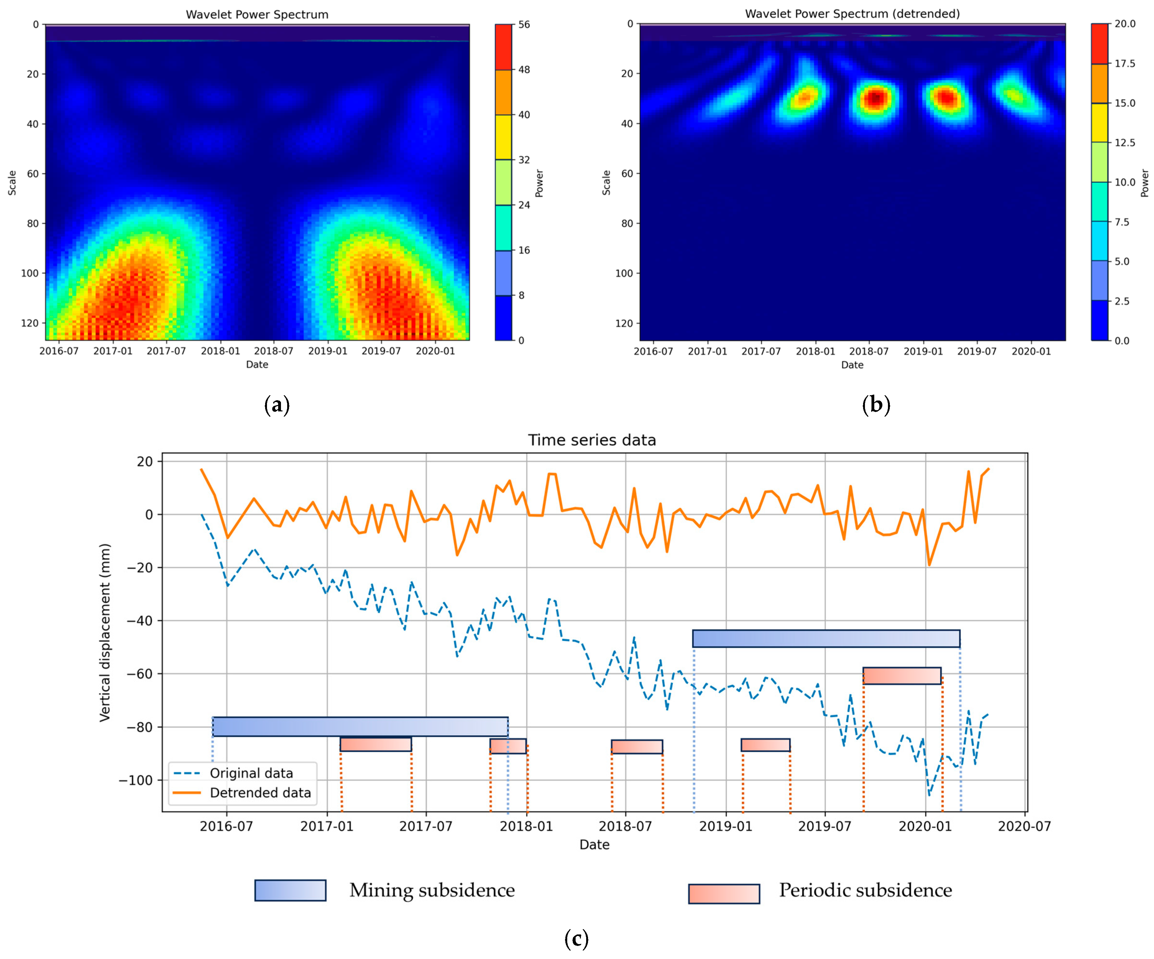
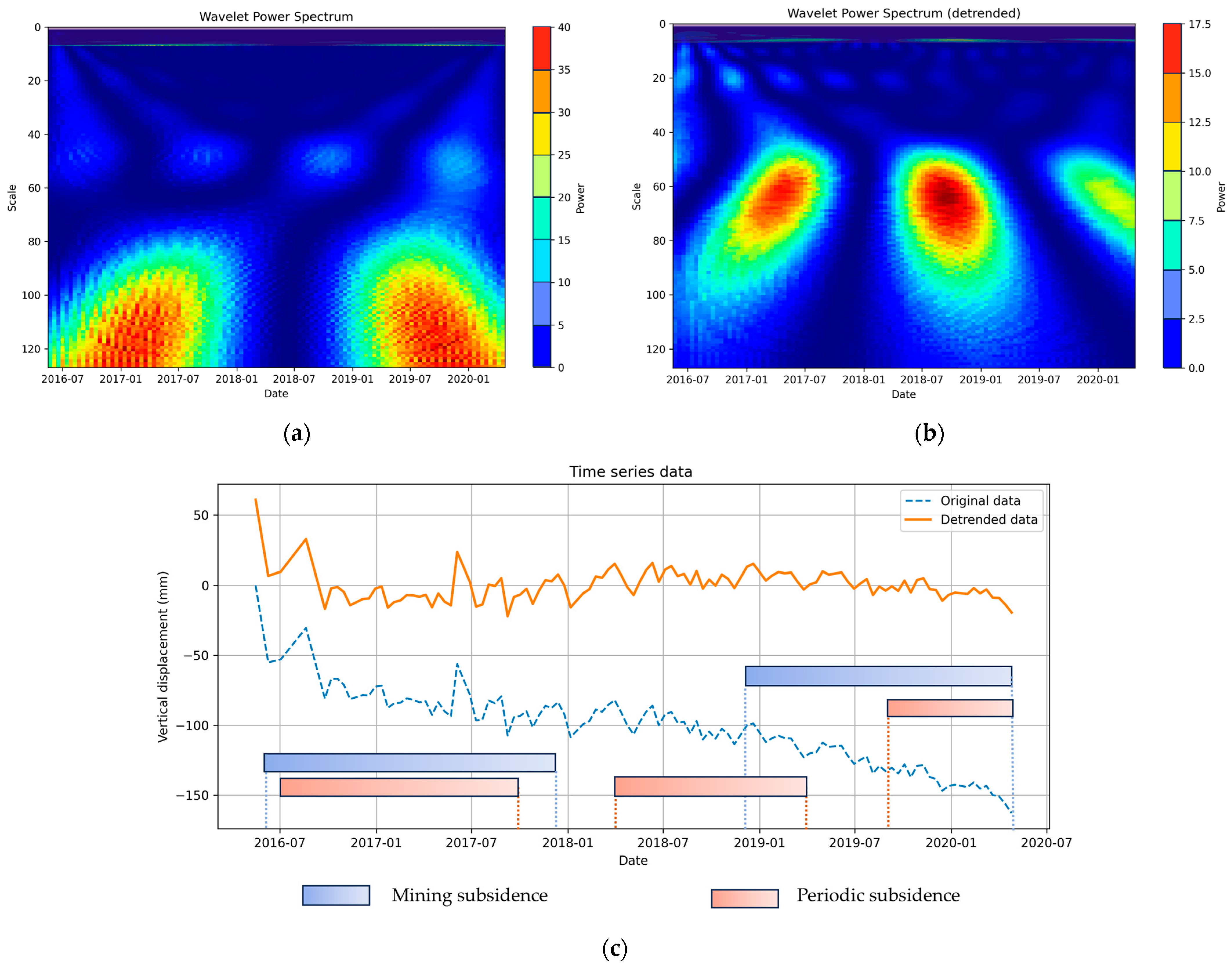
3.2. Wavelet Transform Analysis

To identify significant change points in the time series of surface subsidence induced by underground mining activities, this study employs continuous wavelet transform (CWT) to analyze the local spectral characteristics of the signal. Modulus maxima extraction, red noise background estimation, and significance testing are then applied to detect deformation change points.

The continuous wavelet transform of the time series signal x(t) [44] is defined as follows:

$$W\left(a,b\right)={\int }_{-\mathrm{\infty }}^{\mathrm{\infty }}x\left(t\right){\psi }^{\mathrm{*}}\left({\displaystyle \frac{t-b}{a}}\right)dt$$

(4)

Here, W(a,b) denotes the wavelet transform coefficient at scale a and time offset b; x(t) is the deformation time series; and ψ^∗(t) is the complex conjugate of the mother wavelet function. In this study, the Morlet wavelet is adopted as the mother wavelet [45], and its functional form is given by

$$\psi \left(t\right)={\pi }^{-1/4}{e}^{i{\omega }_{0}t}{e}^{-t^2/2}$$

(5)

Here, ω₀ denotes the central frequency. Typically, ω₀ = 6 is used to achieve a balance between time and frequency resolution. The wavelet power spectrum (WPS), defined as the squared modulus of the wavelet transform coefficient, is used to obtain the energy distribution across different scales.

$$P\left(a,b\right)={\left|W\left(a,b\right)\right|}^2$$

(6)

Due to the scale dependence of the wavelet transform, this study performs scale normalization on the wavelet power spectrum to ensure energy comparability across different scales.

$$\tilde{P}\left(a,b\right)={\displaystyle \frac{{\left|W\left(a,b\right)\right|}^2}{a}}$$

(7)

This normalization ensures that power spectrum values at different scales are not overestimated due to scale effects. To detect change points in deformation signals, this study applies the modulus maxima method to extract the local extrema of wavelet coefficients [46]. The modulus maxima are defined as follows:

$$M\left(a,b\right)=\mathrm{m}\mathrm{a}\mathrm{x}\left(\left|{\displaystyle \frac{\partial W\left(a,b\right)}{\partial b}}\right|\right)$$

(8)

Here, M(a,b) denotes the local extremum of the wavelet transform coefficient at time position b and scale a. In theory, change points correspond to the convergence of modulus maxima across multiple scales along the scale axis.

To ensure the statistical significance of the detected change points, a red noise background power spectrum is constructed, and a 97% confidence level is used for significance testing. Assuming the time series follows a red noise model, its power spectral density P(f) [47] is given by

$$P\left(f\right)={\displaystyle \frac{1-{\alpha }^2}{1-2\alpha \mathrm{c}\mathrm{o}\mathrm{s}\left(2\pi f\right)+{\alpha }^2}}$$

(9)

Here, α is the autoregressive parameter, estimated from the autocorrelation properties of the time series. f represents the normalized frequency. Based on the red noise model, the wavelet power spectrum threshold P_crit(a,b) at the 97% confidence level is calculated to define the significance region.

$$S\left(a,b\right)=\left\{\begin{array}{ll}P\left(a,b\right),& P\left(a,b\right)>P_{\mathrm{crit}}\left(a,b\right)\\ 0,& \mathrm{otherwise}\end{array}\right.$$

(10)

When P(a,b) exceeds the 97% confidence level of the red noise background, the corresponding region is identified as a significant energy enhancement zone and can be used to detect deformation change points [48]. Finally, the wavelet power spectrum is used to analyze energy variations in the deformation time series, and the modulus maxima method is applied to extract change points, further revealing surface subsidence characteristics induced by underground mining.

4. Results

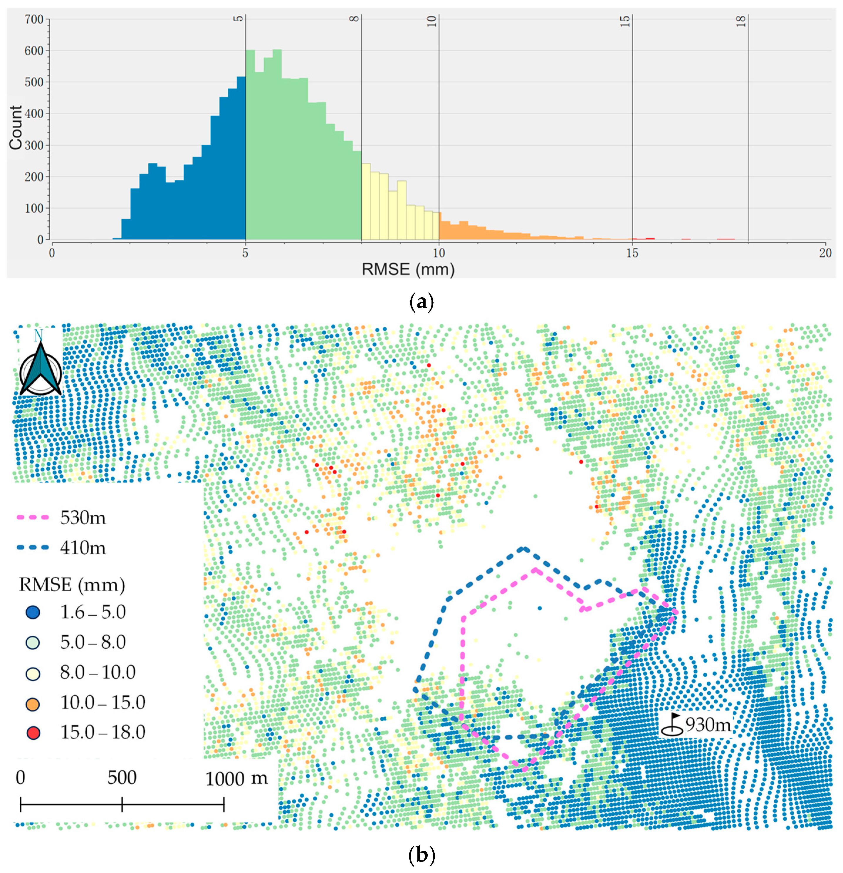
4.1. Subsidence in the Study Area

The cumulative vertical displacement (Figure 7) and vertical deformation rate (Figure 8) of the Tongkuangyu subsidence area from 9 June 2016 to 25 April 2020 were derived using the SBAS-InSAR technique. Since the directly generated maps contain missing values in the central part of the subsidence area, a differential method was used to fill these gaps.

As shown in Figure 7, the maximum settlement displacement on 9 June 2016 was 84.0 mm. On 4 June 2017, the maximum settlement reached 122.1 mm. On 11 June 2018, it increased to 229.3 mm. On 6 June 2019, the value further increased to 275.7 mm. By 25 April 2020, it reached 346.1 mm. The subsidence zone is located in the hanging wall of the ore body. The extent of the subsidence gradually expands over time. The displacement response in the main subsidence area lags behind the timing of ore body excavation. The settlement directly above the goaf continues to increase in the later stages. Subsidence is observed on the southwestern part of the footwall, while uplift occurs on the northeastern side. As shown in Figure 8a, the deformation rate ranges from −81.0 mm/year to 37.3 mm/year during the observation period. The spatial extent of deformation corresponds to that of cumulative settlement. Using a statistical analysis, the annual settlement rates (i.e., all negative values) of all points were extracted, and the 5th percentile was calculated to determine the velocity threshold for severe subsidence across the mining area. The final threshold value is −42.1 mm/year. The reclassified settlement rate map is presented in Figure 8b.

Figure 9 illustrates the spatial and statistical distributions of RMSE across all monitoring points.

As shown in Figure 9a, the RMSE of cumulative displacement data derived from SBAS-InSAR ranges from 1.6 mm to 18 mm, with most monitoring points exhibiting displacement errors between 2 mm and 8 mm. Figure 9b indicates that points with higher RMSE values are predominantly located near the collapse zone.

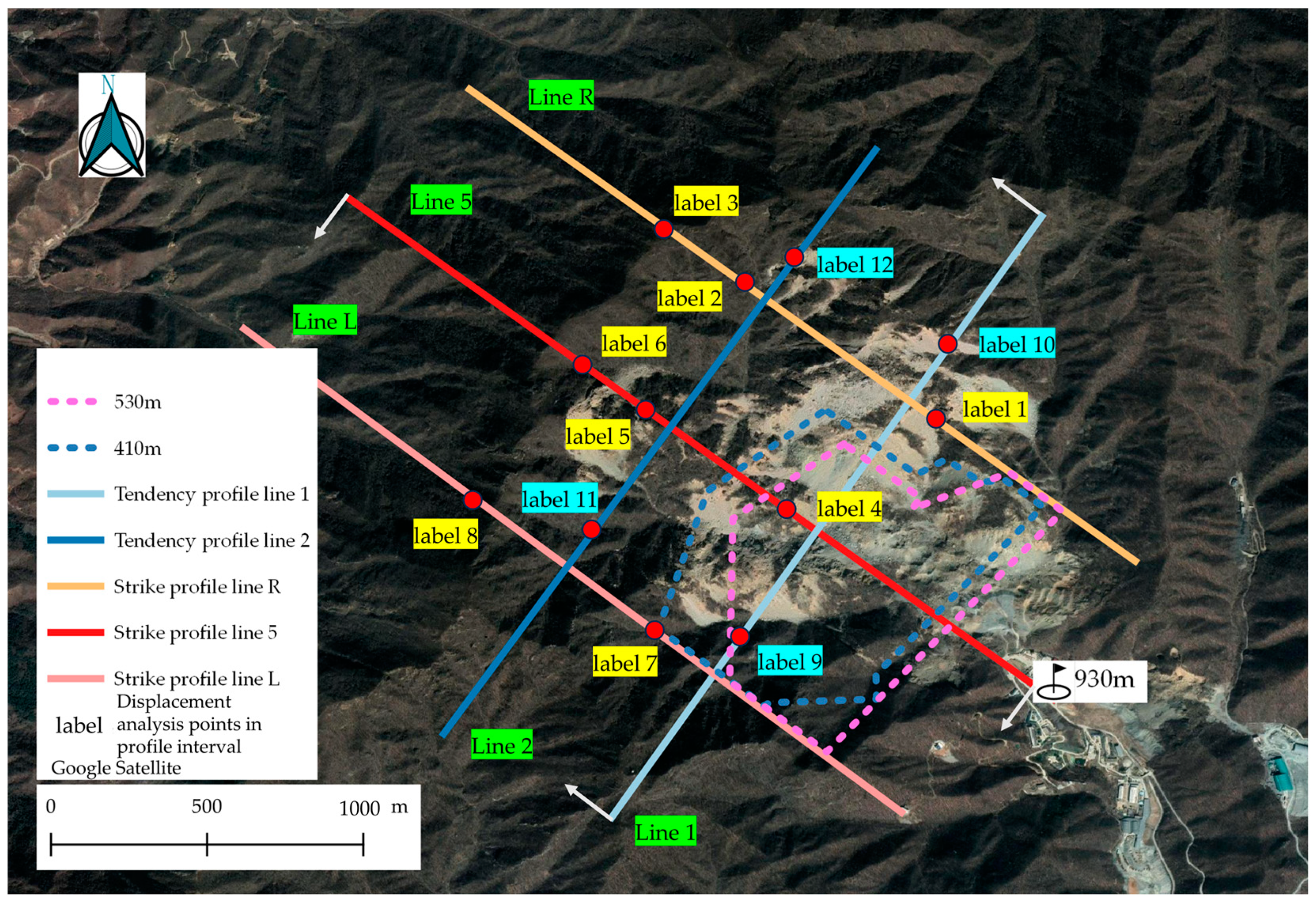
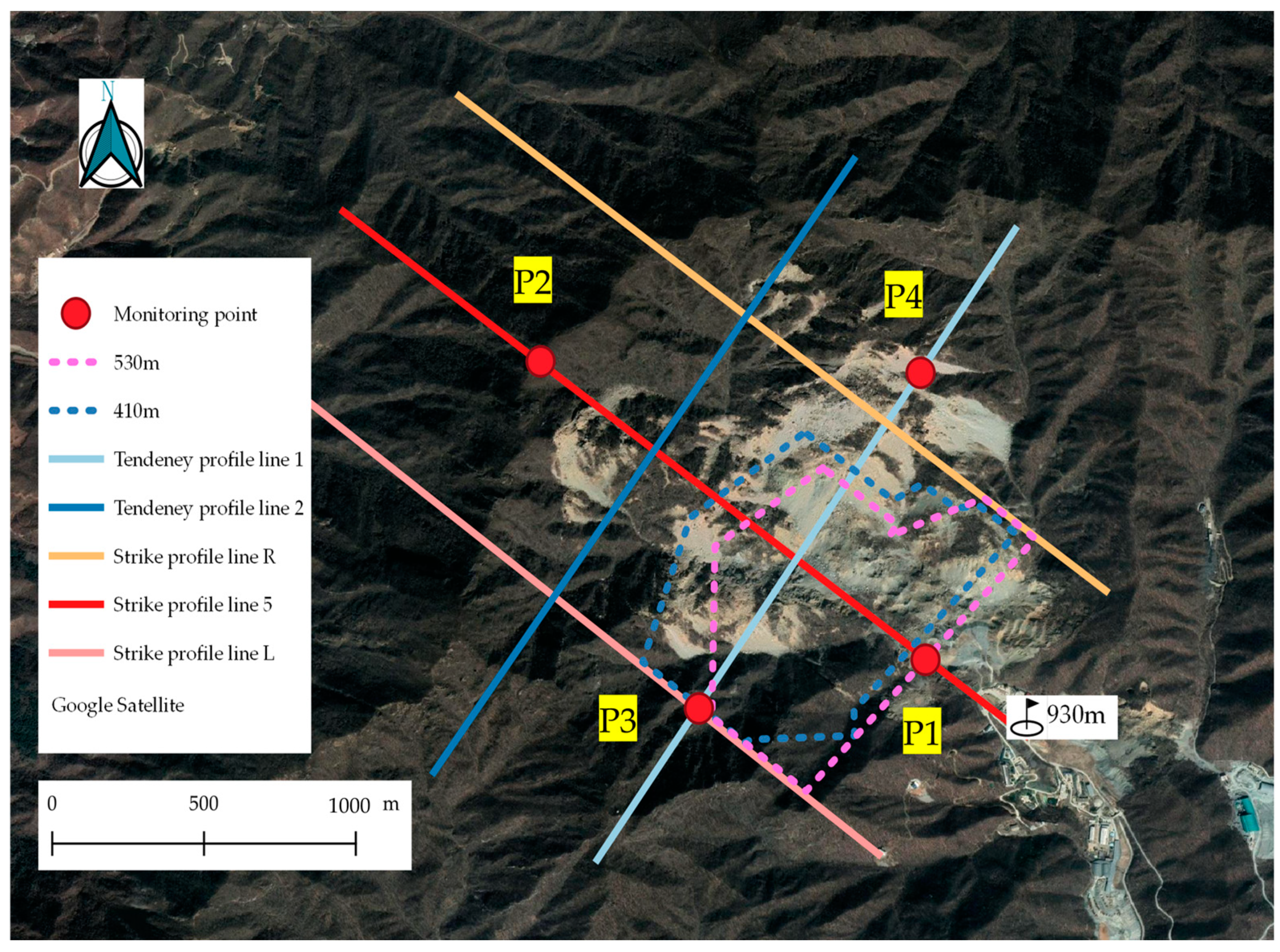
4.2. Settlement Analysis Along Different Profile Lines in the Study Area

To better analyze the settlement characteristics of the Tongkuangyu subsidence area, three profile lines were established perpendicular to the strike of the ore body, and two were aligned along the strike on the hanging wall (Figure 10).

The vertical strike profile lines traverse both the central section and the flanks of the ore body. The surface subsidence displacement time series along profile Line R, Line 5, and Line L are illustrated in Figure 11.

The strike profile Line R, located at the northeastern boundary of the ore body (Figure 11a), shows a maximum settlement of 182.0 mm. A small uplift zone is observed in the western part of the ore body. The settlement between Label 1 and Label 2 is comparable. Satellite imagery reveals a clearly exposed rock surface in this area, likely resulting from a landslide. However, significant increases in settlement were observed from June to December in both 2017 and 2019, compared to the preceding years. Between Label 2 and Label 3 lies another hillside, where the settlement is considerably smaller.

In the central strike profile, Line 5 (Figure 11b), the maximum settlement reaches 199.9 mm. Southeast of Label 4, between Label 4 and Label 5, the settlement in the two segments is relatively consistent, with greater displacement observed in the second half of each year compared to the first half. The largest settlement occurs between Label 5 and Label 6. Satellite imagery reveals clear evidence of collapse and landslides between Label 4 and Label 6.

The strike profile Line L, located at the southwestern boundary of the ore body (Figure 11c), exhibits a maximum settlement of 243.6 mm. Between Label 7 and Label 8, the settlement trend remains stable, with no significant year-to-year increase observed. No distinct exposed rock zones are visible in the satellite imagery.

Based on the data from the three profile lines perpendicular to the ore body strike, settlement in the southwestern part of the subsidence area is greater than that in the northeastern part.

The tendency profile line spans the main collapse zone located on the hanging wall of the ore body. The surface subsidence displacement time series along tendency profile Lines 1 and 2 are illustrated in Figure 12.

For tendency profile Line 1 (Figure 12a), the maximum recorded settlement is 262.2 mm. Between Label_9 and Label_10, satellite imagery reveals a clearly defined collapse zone. In the Label_9 area, the settlement from June to December 2019 increased relative to the same period in previous years. In the Label_10 area, the settlement began to accelerate after the end of 2018 relative to previous years. Overall, the onset of settlement in the western section lags approximately six months behind that in the eastern section.

For tendency profile Line 2 (Figure 12b), the maximum settlement reaches 241.7 mm. Satellite imagery shows a collapse trace between Label_11 and Label_12. Overall, the settlement in the western section is greater than in the eastern section. Temporally, in the Label_11 area, the settlement decreased in June 2018 compared to the first half of the year. During other periods, the settlement rate remained relatively constant, indicating overall stability. In the Label_12 area, the settlement increased in both December 2016 and December 2017 relative to the first half of each respective year.

Based on the data from the two strike-parallel profile lines, the annual settlement in the western part of the subsidence area remains relatively stable, while the eastern part exhibits occasional sudden increases.

Based on the data from all integrated profile lines, it can be inferred that the settlement in the southwestern part of the subsidence area is relatively large and increases steadily each year. In contrast, the northeastern part exhibits both sudden increases and decreases in settlement.

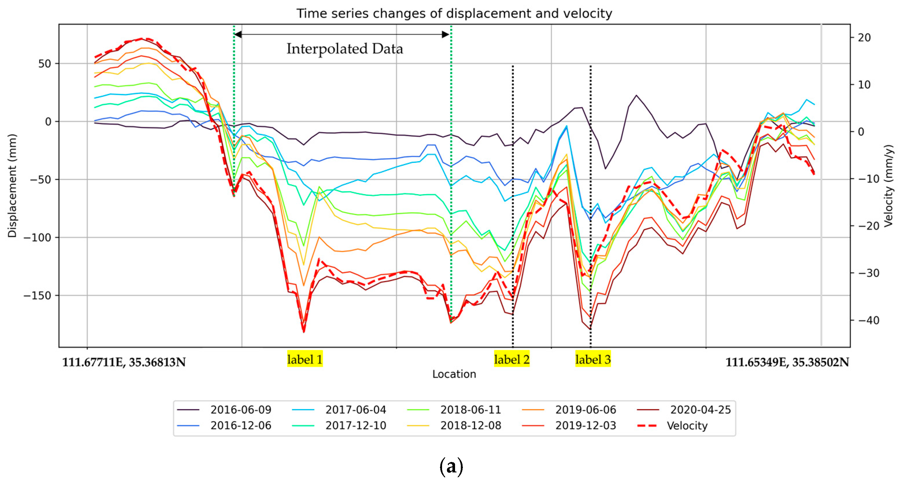
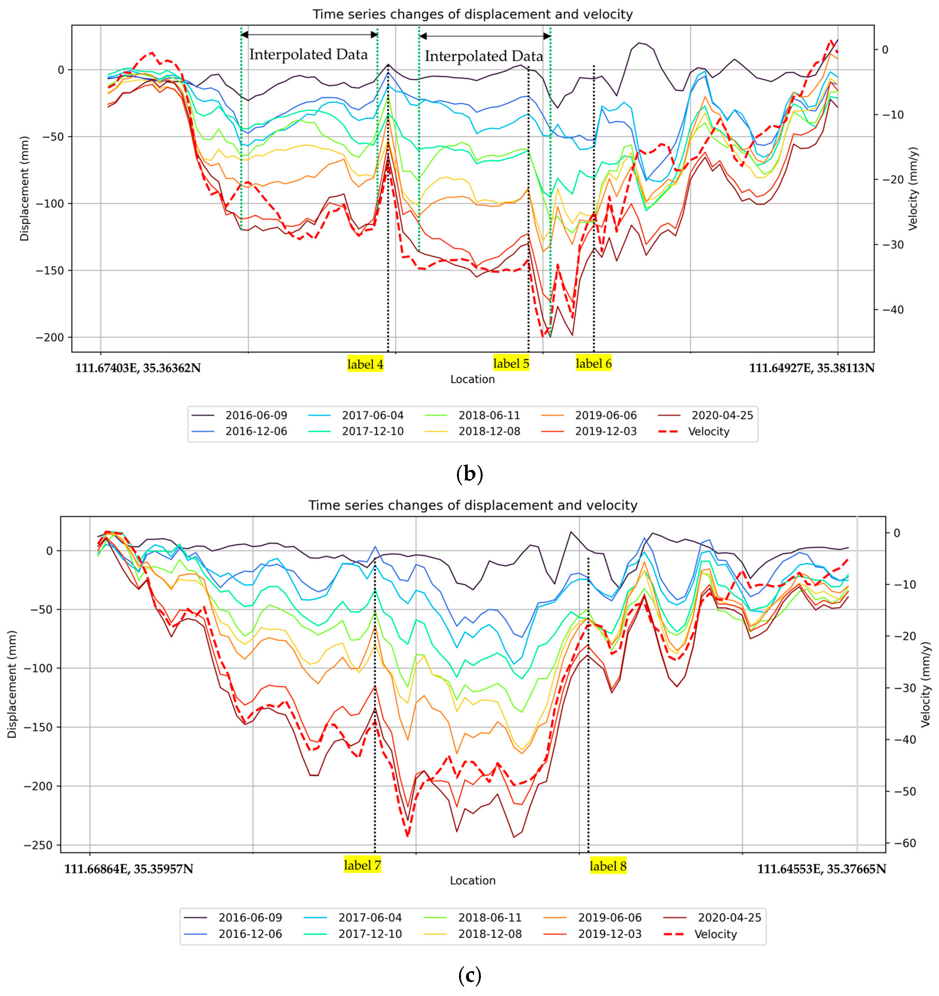
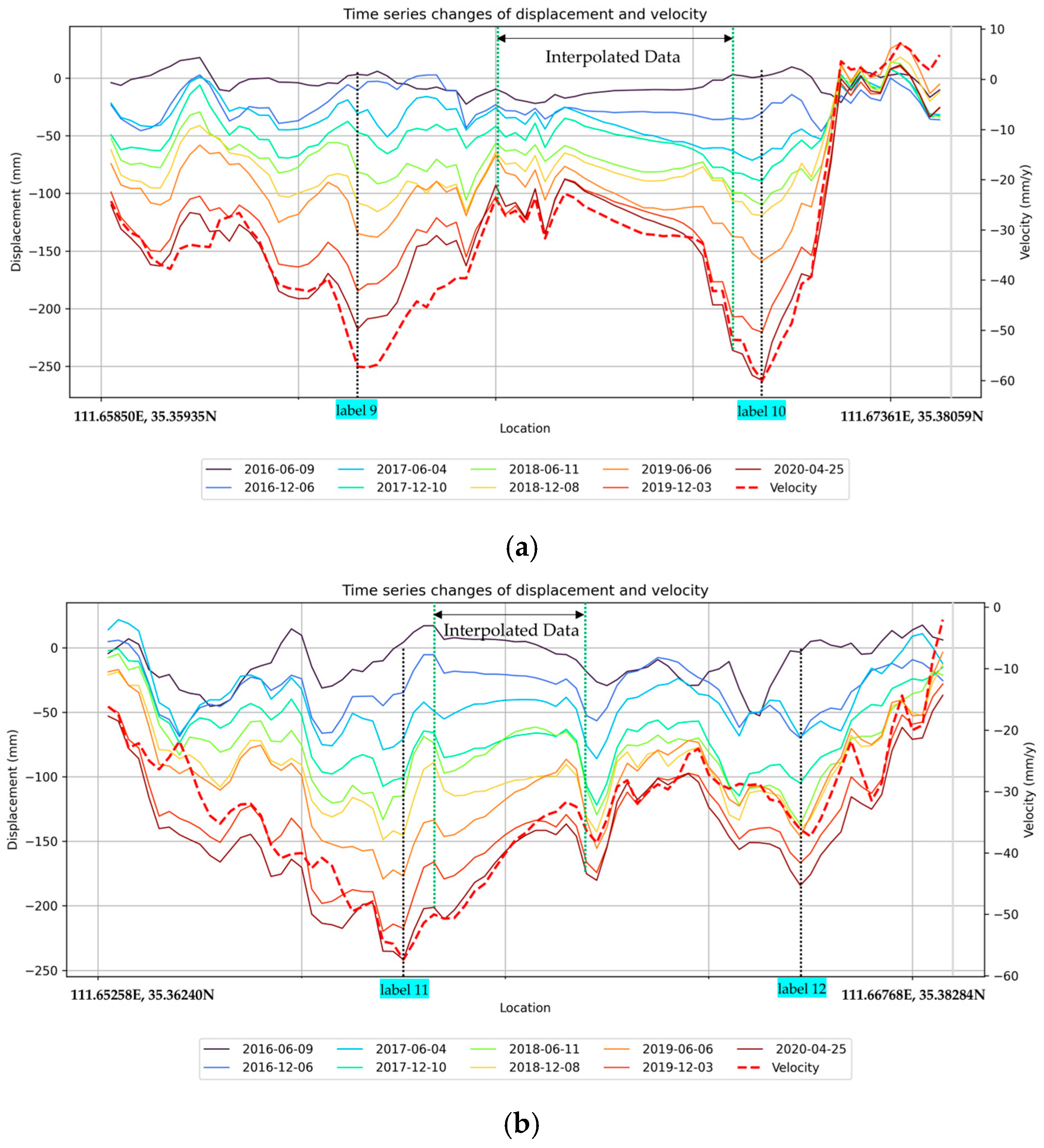
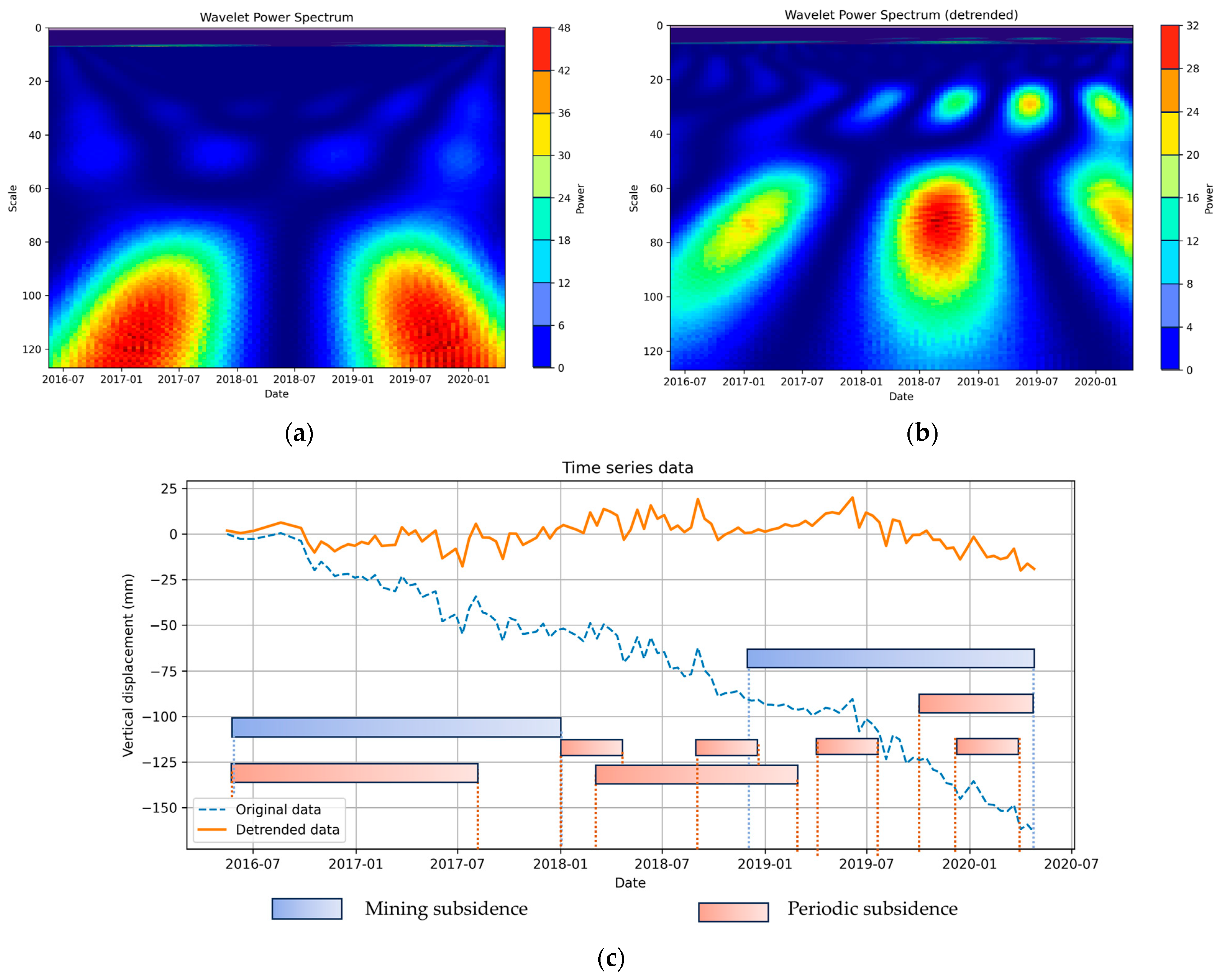
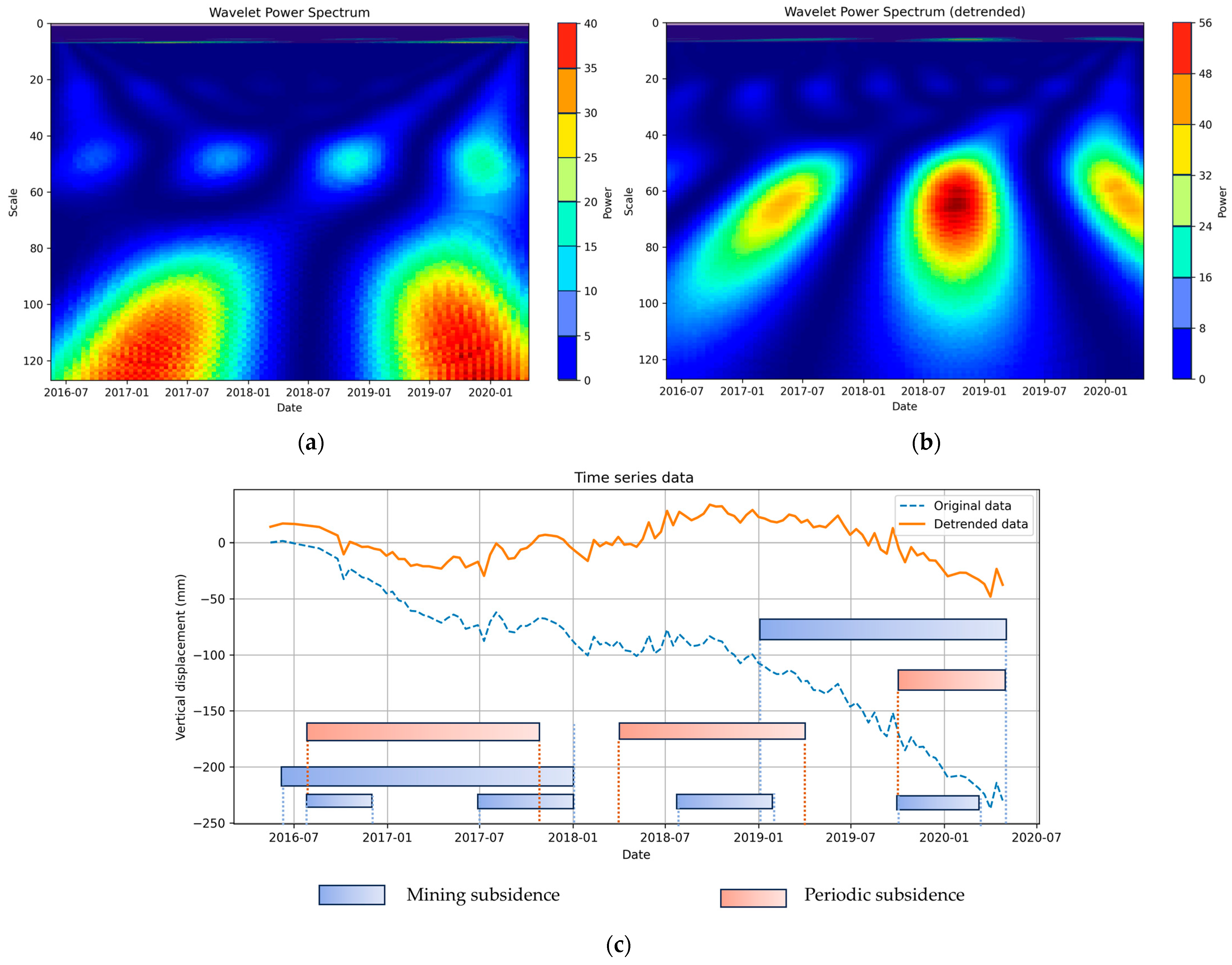
4.3. Analysis of Sudden Changes in Settlement Rates at Various Locations Within the Study Area

An analysis of the settlement displacement and rate across the overall subsidence area and along individual profile lines reveals distinct subsidence characteristics in different zones. To further investigate the subsidence behavior—specifically whether it is driven by external periodic factors or the sustained influence of mining activities—a wavelet power spectrum analysis is applied to the subsidence displacement time series. Four reference points were selected around the subsidence area (Figure 13). The settlement time series for each point was divided into original and detrended components. The time series data were normalized, filtered, and smoothed to minimize the impact of noise. Continuous wavelet transform (CWT) was applied to compute the wavelet power spectrum (WPS).

The wavelet power spectra and settlement displacement time series for each reference point are shown in Figure 14, Figure 15, Figure 16 and Figure 17.

In the wavelet power spectrum, the X-axis (Date) spans from 2016 to 2020, representing the temporal evolution of displacement data. The Y-axis (Scale) denotes the wavelet scale, which reflects signal variations across different temporal resolutions. Small scales (upper region, <40) correspond to short-term variations, such as monthly fluctuations. Medium scales (middle region, 40–80) correspond to intermediate-term variations, such as quarterly or semiannual fluctuations. Large scales (lower region, >80) reflect long-term changes, including interannual or multi-year trends. The color scale indicates the wavelet power (Power). Dark blue regions (indicating low power) suggest weak signals at the corresponding time scales, implying no significant settlement anomalies during those periods. Yellow-to-red regions (indicating high power) highlight strong signal responses at specific scales, potentially corresponding to abrupt changes or significant periodic fluctuations.

Reference point P1 is located east of the 530 m mining boundary. Figure 14a presents the wavelet power spectrum of the original time series data. Two high-power regions (yellow to red) are observed at scales of 80–120 during the periods from June 2016 to December 2017 and from November 2018 to April 2020, indicating significant settlement anomalies during these intervals. These anomalies may be associated with mining or geological activities in the area, leading to substantial surface displacements. The scale of the earlier high-power region gradually decreases, suggesting a shortening duration of settlement. In contrast, the scale of the later high-power region increases over time, implying a progressive accumulation of settlement. At small to medium scales (20–60), regularly spaced blue intervals are observed, showing monthly or quarterly alternations, which may suggest the presence of a short-period settlement pattern in this area.

Figure 14b presents the wavelet power spectrum of the detrended data. Compared with the original data, the detrended version eliminates the influence of long-term trends, allowing for a clearer focus on periodic settlement patterns. At approximately scale 30, high-power regions (yellow to red) appear during five distinct periods: February–June 2017, November 2017–January 2018, June–September 2018, February–May 2019, and September 2019–February 2020, indicating the presence of periodic settlement during these intervals.

The time series data and corresponding mutation intervals for reference point P1 are shown in Figure 14c. The displacement at this point exhibits an overall increasing trend, with an average settlement rate of 20.1 mm/year over the five-year period.

Reference point P2 is located on the hanging wall of the ore body, in the northwestern part of the collapse zone. Figure 15a presents the wavelet power spectrum of the original time series data. Two high-power regions (yellow to red) are observed at scales of 80–120 during the periods June 2016–December 2017 and December 2018–April 2020. These patterns are consistent with those observed at reference point P1. At the mesoscale (approximately scale 50), intermittent moderate-power fluctuations (blue–green) occur in a semiannual alternating pattern. Compared to reference point P1 on the footwall, these findings suggest that the interval between settlement events on the hanging wall is relatively longer.

Figure 15b presents the wavelet power spectrum of the detrended data. From July 2016 to October 2017 and from April 2018 to April 2019, high-power regions (yellow to red) appear at scales of 40–100, indicating significant settlement anomalies during these periods. Between September 2019 and April 2020, moderate-to-high power (yellow–green) is observed at scales of 60–80. Temporally, this follows the two earlier high-power regions, suggesting a longer-term accumulation of settlement deformation beginning after September 2019. Overall, compared to the footwall reference point P1, the hanging wall exhibits greater settlement magnitude and longer duration.

The time series data and corresponding mutation intervals for reference point P2 are shown in Figure 15c. The displacement at this point exhibits an overall increasing trend, with an average settlement rate of 22.1 mm/year over the five-year period.

Reference point P3 is located on the southwestern wing of the hanging wall of the ore body, within the subsidence area. Figure 16a presents the wavelet power spectrum of the original time series data. Two high-power regions (yellow to red) are observed at scales of 80–120 during the periods June 2016–January 2018 and December 2018–April 2020. These patterns are consistent with those observed at reference points P1 and P2. At the mesoscale (around scale 50), intermittent moderate- and low-power fluctuations (blue) occur in a semiannual alternating pattern. This behavior is similar to that of the hanging wall reference point P2, although the fluctuation intensity is weaker; however, it remains stronger than that observed at reference point P1.

Figure 16b presents the wavelet power spectrum of the detrended data. Three high-power periods (yellow to red) are observed at scales of 50–120 during April 2016–August 2017, March 2018–March 2019, and October 2019–April 2020, indicating substantial settlement anomalies during these intervals. After January 2018, medium-to-high power (green to red) appears at scales of 20–40. Temporally, this pattern begins with the second anomaly and persists for approximately four months, suggesting that after March 2018, there is sustained settlement accumulation accompanied by a notable change in the displacement rate. Overall, the western wing of the subsidence area appears to be strongly influenced by periodic mining activities, with deformation persisting over extended periods.

The time series data and corresponding abrupt change intervals for reference point P3 are shown in Figure 16c. The displacement at this point exhibits a consistent increasing trend over time, with an average settlement rate of 38.0 mm/year over the five-year period.

Reference point P4 is located on the northeastern wing of the hanging wall of the ore body, within the collapse zone. Figure 17a presents the wavelet power spectrum of the original time series data. Two high-power regions (yellow to red) are observed at scales of 80–120 during June 2016–January 2018 and January 2019–April 2020. These patterns are consistent with those observed at reference points P1, P2, and P3. At the mesoscale (around scale 50), intermittent moderate- and low-power fluctuations (blue–green) occur in a semiannual alternating pattern. This behavior is similar to that at reference points P2 and P3, but with greater fluctuation intensity.

Figure 17b presents the wavelet power spectrum of the detrended data. Three high-power periods (yellow to red) are observed at scales of 40–100 during August 2016–November 2017, April 2018–April 2019, and October 2019–April 2020, indicating significant settlement anomalies during these intervals. Around scale 30, continuous low-power fluctuations with relatively weak intensity are observed, occurring on a monthly basis. This suggests the presence of persistent minor displacement variations in the area.

The time series data and corresponding mutation intervals for reference point P4 are shown in Figure 17c. The displacement at this point exhibits a clear upward trend over time. The average settlement rate over the five-year period is 47.6 mm/year.

A wavelet analysis reveals that in addition to long-term settlement induced by mining activities, periodic settlement patterns also exist in the subsidence area. A comparative analysis indicates that periodic subsidence is not directly correlated with rainfall. Instead, it is primarily attributed to cumulative subsidence induced by periodic mining activities.

When delineating high-risk subsidence zones, relying solely on the threshold of the annual average deformation rate may overlook short-term anomalies (i.e., instantaneous accelerations), such as sudden collapses or landslides triggered by geological structures or activities. Therefore, it is necessary to quantify the number of regional mutation points to identify areas that are more susceptible to sudden surface deformation. Significant mutation points are identified by computing the gradient of the displacement time series at each location, extracting the maximum modulus values, modeling the red noise background, and applying a 97% quantile threshold.

The calculated maximum mutation rates are 38.9 mm/day for reference point P1, 49.1 mm/day for P2, 19.1 mm/day for P3, and 30.9 mm/day for P4. The number of significant mutation points is determined for the top 10% of each settlement time series. Finally, a heat map illustrating the spatial distribution of regional mutation point density is generated using QGIS 3.16 (Figure 18). Red areas indicate regions with more frequent sudden surface deformations. The image also shows that these red regions correspond to the core subsidence zones, where evident landslide activity is present.

5. Discussion

This study utilizes SBAS-InSAR to obtain historical subsidence data in mining-affected areas, effectively compensating for the lack of early-stage displacement monitoring and offering a new, safe, and efficient method for the long-term monitoring of subsidence regions. As underground mining is a long-term and systematic process, the formation of goafs follows a relatively predictable pattern. Surface subsidence is influenced not only by the spatial and temporal development of goafs, but also by external environmental factors. Furthermore, geological subsidence often lags behind the formation of goafs. In this study, a wavelet analysis is employed to transform the subsidence displacement time series into wavelet power spectra, leveraging its excellent time–frequency localization and capability in detecting abrupt signal changes. This enables the clear and intuitive identification of subsidence mutation periods in the affected areas. In summary, this study offers an important scientific reference for the safety management of mining subsidence areas. Compared with previous analysis methods, it fully utilizes limited data, delineates subsidence areas by considering multiple subsidence patterns, and offers new insights and approaches for studying similar subsidence regions.

It is important to note that when SBAS-InSAR is applied to monitor surface displacement in underground metal mine goafs, the resulting raster images often contain data voids in the core subsidence zones. In this study, the natural neighbor interpolation method is employed to fill in these voids. Although this approach allows for the supplementation of missing data in core subsidence areas, the interpolated values are not actual measurements and therefore introduce certain limitations in the analysis of these zones. In the analysis of displacement and velocity along the profile lines shown in Figure 10 and Figure 11, the ranges of differential data have been explicitly marked. As the primary objective of this study is to delineate high-risk surface subsidence boundaries using both long-term and short-term settlement velocity thresholds as criteria, the application of natural neighbor interpolation not only ensures spatial data continuity, but also does not negatively affect the overall research outcomes.

In addition to ongoing mining activities, surface subsidence is also influenced by factors such as the lithological properties of underlying rock layers, geological structures, and hydrological conditions, each exerting varying degrees of impact. However, the goaf formed by mining remains the primary driver of subsidence. It not only alters the stress distribution around the rock mass—leading to the failure of weak rock strata and structural planes—but may also induce drainage from underground water-rich layers into the goaf, thereby changing the physical state of overlying strata.

This study employs a wavelet analysis to identify the fundamental patterns of ground subsidence in collapse-prone areas. The results reveal both long-term subsidence driven by underground cavity formation and periodic subsidence influenced by multiple factors, offering valuable insights for predicting potential expansion of collapse zones. However, due to the unavailability of reliable geological structure and groundwater level data, only the overall subsidence trend in the collapse area can be analyzed, and the detailed decomposition of periodic subsidence remains infeasible.

After conducting detailed investigations into lithology, geological structures, hydrogeology, and related data in the future, a more comprehensive analysis of the factors influencing subsidence can be performed. Meanwhile, a multi-factor prediction model for subsidence areas can be developed to provide high-precision predictions of the range of surface subsidence caused by future mining activities.

6. Conclusions

This study aims to monitor surface displacement and analyze settlement patterns associated with subsidence induced by underground metal mining, with the objective of delineating high-risk subsidence zones. SBAS-InSAR technology is employed to obtain millimeter-level surface displacement data for the collapse area from June 9, 2016, to April 25, 2020, with a 12-day temporal resolution. Compared to traditional monitoring methods, SBAS-InSAR does not require the pre-installation of ground-based measuring points or on-site surveys, thereby reducing manpower and material costs while enhancing operational safety. Temporally, Sentinel-1 data are available dating from as early as 2014, allowing historical displacement patterns during ore extraction to be traced and enabling long-term time series analysis.

The results indicate that from June 2016 to April 2020, the annual maximum cumulative settlement in the collapse area was 84.0 mm, 122.1 mm, 229.3 mm, 275.7 mm, and 346.1 mm, respectively. Based on a comprehensive analysis of profile line data, the southwestern part of the collapse area exhibits relatively large and steadily increasing settlement over the years. In contrast, the northeastern area shows abrupt increases and decreases in settlement. The maximum observed settlement rate in the study area is −81.0 mm/year. A statistical analysis determines a critical settlement rate threshold of −42.1 mm/year for identifying severely affected zones across the mining area.

To explore settlement patterns in the collapse area, continuous wavelet transform (CWT) is applied for its excellent time-frequency localization capabilities. Mutation point detection is performed to separate trend components from periodic fluctuations in the collapse rate and to classify settlement patterns across different time periods.

In the absence of historical monitoring data for the collapse area of the Tongkuangyu Mine, the application of the SBAS-InSAR technique provides a safe and efficient means of acquiring reliable cumulative displacement and settlement rate data. By applying an annual average settlement rate threshold, zones of severe long-term subsidence can be effectively identified. A wavelet analysis, combined with an instantaneous displacement rate threshold, enables the detection of short-term fluctuating subsidence areas. The combination of both thresholds allows for the accurate delineation of high-risk subsidence zones, offering a novel and effective approach for identifying surface collapse areas induced by underground metal mining. Building on this study, the future integration of multi-source datasets with methods such as machine learning and numerical simulation may enable the accurate prediction of settlement trends and the spatial expansion of collapse areas.

References

1. Niu, X.; Hou, K.; Bao, G.; Zhe, Y. Study on Formation Mechanism of Mud-Inclusion-Type Underground Debris Flows Using Natural Caving Method. Sci. Rep. 2024, 14, 4324. [Google Scholar] [CrossRef] [PubMed]
2. Lee, S.; Park, I. Application of Decision Tree Model for the Ground Subsidence Hazard Mapping near Abandoned Underground Coal Mines. J. Environ. Manag. 2013, 127, 166–176. [Google Scholar] [CrossRef]
3. GUO, W.; HOU, Q.; ZOU, Y. Relationship between Surface Subsidence Factor and Mining Depth of Strip Pillar Mining. Trans. Nonferrous Met. Soc. China 2011, 21, s594–s598. [Google Scholar] [CrossRef]
4. Sheorey, P.R.; Loui, J.P.; Singh, K.B.; Singh, S.K. Ground Subsidence Observations and a Modified Influence Function Method for Complete Subsidence Prediction. Int. J. Rock Mech. Min. Sci. 2000, 37, 801–818. [Google Scholar] [CrossRef]
5. Hu, J.; Zhang, X.; Yan, M.; Bai, L.; Wang, S.; Wang, B.; Liu, J.; Gao, Y. Cyclic Loading Changes the Taproot’s Tensile Properties and Reinforces the Soil via the Shrub’s Taproot in Semi-Arid Areas, China. Sci. Rep. 2024, 14, 2281. [Google Scholar] [CrossRef] [PubMed]
6. Wang, J.; Lu, C.; Sun, Q.; Xiao, W.; Cao, G.; Li, H.; Yan, L.; Zhang, B. Simulating the Hydrologic Cycle in Coal Mining Subsidence Areas with a Distributed Hydrologic Model. Sci. Rep. 2017, 7, 39983. [Google Scholar] [CrossRef]
7. Salles, R.; Belloze, K.; Porto, F.; Gonzalez, P.H.; Ogasawara, E. Nonstationary Time Series Transformation Methods: An Experimental Review. Knowl.-Based Syst. 2019, 164, 274–291. [Google Scholar] [CrossRef]
8. Yang, Y.; Peng, Z.K.; Dong, X.J.; Zhang, W.M.; Meng, G. General Parameterized Time-Frequency Transform. IEEE Trans. Signal. Process. 2014, 62, 2751–2764. [Google Scholar] [CrossRef]
9. Lian, X.; Shi, L.; Kong, W.; Han, Y.; Fan, H. Residual Subsidence Time Series Model in Mountain Area Caused by Underground Mining Based on GNSS Online Monitoring. Int. J. Coal Sci. Technol. 2024, 11, 27. [Google Scholar] [CrossRef]
10. Zheng, J.; Yao, W.; Lin, X.; Ma, B.; Bai, L. An Accurate Digital Subsidence Model for Deformation Detection of Coal Mining Areas Using a UAV-Based LiDAR. Remote Sens. 2022, 14, 421. [Google Scholar] [CrossRef]
11. Fan, H.; Wang, L.; Wen, B.; Du, S. A New Model for Three-Dimensional Deformation Extraction with Single-Track InSAR Based on Mining Subsidence Characteristics. Int. J. Appl. Earth Obs. Geoinf. 2021, 94, 102223. [Google Scholar] [CrossRef]
12. Yang, Z.; Li, Z.; Zhu, J.; Yi, H.; Hu, J.; Feng, G. Deriving Dynamic Subsidence of Coal Mining Areas Using InSAR and Logistic Model. Remote Sens. 2017, 9, 125. [Google Scholar] [CrossRef]
13. Xie, M.; Huang, J.; Wang, L.; Huang, J.; Wang, Z. Early Landslide Detection Based on D-InSAR Technique at the Wudongde Hydropower Reservoir. Environ. Earth Sci. 2016, 75, 717. [Google Scholar] [CrossRef]
14. Liu, Y.; Li, L.; Yang, J.; Chen, X.; Hao, J. Estimating Snow Depth Using Multi-Source Data Fusion Based on the D-InSAR Method and 3DVAR Fusion Algorithm. Remote Sens. 2014, 9, 1195. [Google Scholar] [CrossRef]
15. Singleton, A.; Li, Z.; Hoey, T.; Muller, J.-P.; Liu, Y.; Li, L.; Yang, J.; Chen, X.; Hao, J. Evaluating Sub-Pixel Offset Techniques as an Alternative to D-InSAR for Monitoring Episodic Landslide Movements in Vegetated Terrain. Remote Sens. Environ. 2014, 147, 133–144. [Google Scholar] [CrossRef]
16. Li, Y.; Zuo, X.; Yang, F.; Bu, J.; Wu, W.; Liu, X. Effectiveness Evaluation of DS-InSAR Method Fused PS Points in Surface Deformation Monitoring: A Case Study of Hongta District, Yuxi City, China. Geomat. Nat. Hazards Risk 2023, 14, 2176011. [Google Scholar] [CrossRef]
17. Sousa, J.J.; Ruiz, A.M.; Hanssen, R.F.; Bastos, L.; Gil, A.J.; Galindo-Zaldívar, J.; Sanz de Galdeano, C. PS-InSAR Processing Methodologies in the Detection of Field Surface Deformation—Study of the Granada Basin (Central Betic Cordilleras, Southern Spain). J. Geodyn. 2010, 49, 181–189. [Google Scholar] [CrossRef]
18. Zhang, P.; Guo, Z.; Guo, S.; Xia, J. Land Subsidence Monitoring Method in Regions of Variable Radar Reflection Characteristics by Integrating PS-InSAR and SBAS-InSAR Techniques. Remote Sens. 2022, 14, 3265. [Google Scholar] [CrossRef]
19. Zhang, L.; Dai, K.; Deng, J.; Ge, D.; Liang, R.; Li, W.; Xu, Q. Identifying Potential Landslides by Stacking-InSAR in Southwestern China and Its Performance Comparison with SBAS-InSAR. Remote Sens. 2021, 13, 3662. [Google Scholar] [CrossRef]
20. Yalvac, S. Validating InSAR-SBAS Results by Means of Different GNSS Analysis Techniques in Medium- and High-Grade Deformation Areas. Environ. Monit. Assess. 2020, 192, 120. [Google Scholar] [CrossRef]
21. Xu, Y.; Li, T.; Tang, X.; Zhang, X.; Fan, H.; Wang, Y. Research on the Applicability of DInSAR, Stacking-InSAR and SBAS-InSAR for Mining Region Subsidence Detection in the Datong Coalfield. Remote Sens. 2022, 14, 3314. [Google Scholar] [CrossRef]
22. Lee, D.-K.; Mojtabai, N.; Lee, H.-B.; Song, W.-K. Assessment of the Influencing Factors on Subsidence at Abandoned Coal Mines in South Korea. Environ. Earth Sci. 2013, 68, 647–654. [Google Scholar] [CrossRef]
23. Xiao, H.; Xia, Y.; Fan, Y.; Chen, L.; Duan, R. Identification and Prediction Inversion of Mining Area Subsidence by Integrating SBAS-InSAR and EMD-ARIMA Model. IEEE Access 2024, 12, 85822–85835. [Google Scholar] [CrossRef]
24. Li, N.; Liu, D.; Wang, L.; Ye, H.; Wang, Q.; Yan, D.; Zhao, S. Combination Prediction of Underground Mine Rock Drilling Time Based on Seasonal and Trend Decomposition Using Loess. Eng. Appl. Artif. Intell. 2024, 133, 108064. [Google Scholar] [CrossRef]
25. Chen, B.Q.; Deng, K.Z. Integration of D-InSAR Technology and PSO-SVR Algorithm for Time Series Monitoring and Dynamic Prediction of Coal Mining Subsidence. Surv. Rev. 2014, 46, 392–400. [Google Scholar] [CrossRef]
26. Xu, J.; Yan, C.; Zhang, B.; Chen, X.; Yan, X.; Wang, R.; Yu, B.; Boota, M.W. Investigation of Spatio-Temporal Simulation of Mining Subsidence and Its Determinants Utilizing the RF-CA Model. Land 2025, 14, 268. [Google Scholar] [CrossRef]
27. Liu, Y.; Zhang, J. Integrating SBAS-InSAR and AT-LSTM for Time-Series Analysis and Prediction Method of Ground Subsidence in Mining Areas. Remote Sens. 2023, 15, 3409. [Google Scholar] [CrossRef]
28. Zhang, J.; Gao, J.; Gao, F. Time Series Land Subsidence Monitoring and Prediction Based on SBAS-InSAR and GeoTemporal Transformer Model. Earth Sci. Inform. 2024, 17, 5899–5911. [Google Scholar] [CrossRef]
29. Yuan, M.; Li, M.; Liu, H.; Lv, P.; Li, B.; Zheng, W. Subsidence Monitoring Base on SBAS-InSAR and Slope Stability Analysis Method for Damage Analysis in Mountainous Mining Subsidence Regions. Remote Sens. 2021, 13, 3107. [Google Scholar] [CrossRef]
30. Chen, X.; Chen, J.; Wang, G.; Zhang, Q.; Zheng, Y. Mining Subsidence Based on Integrated SBAS-InSAR and Unmanned Aerial Vehicles Technology. J. Ocean Univ. China 2025, 24, 113–129. [Google Scholar] [CrossRef]
31. Chen, Y.; Yu, S.; Tao, Q.; Liu, G.; Wang, L.; Wang, F. Accuracy Verification and Correction of D-InSAR and SBAS-InSAR in Monitoring Mining Surface Subsidence. Remote Sens. 2021, 13, 4365. [Google Scholar] [CrossRef]
32. Tomás, R.; Li, Z.; Lopez-Sanchez, J.M.; Liu, P.; Singleton, A. Using Wavelet Tools to Analyse Seasonal Variations from InSAR Time-Series Data: A Case Study of the Huangtupo Landslide. Landslides 2016, 13, 437–450. [Google Scholar] [CrossRef]
33. Meng, X.; Richards, J.; Mao, J.; Ye, H.; DuFrane, S.A.; Creaser, R.; Marsh, J.; Petrus, J. The Tongkuangyu Cu Deposit, Trans-North China Orogen: A Metamorphosed Paleoproterozoic Porphyry Cu Deposit. Econ. Geol. 2020, 115, 51–77. [Google Scholar] [CrossRef]
34. Li, S.; Xu, W.; Li, Z. Review of the SBAS InSAR Time-Series Algorithms, Applications, and Challenges. Geod. Geodyn. 2022, 13, 114–126. [Google Scholar] [CrossRef]
35. Osmanoğlu, B.; Sunar, F.; Wdowinski, S.; Cabral-Cano, E. Time Series Analysis of InSAR Data: Methods and Trends. ISPRS J. Photogramm. Remote Sens. 2016, 115, 90–102. [Google Scholar] [CrossRef]
36. Yu, Z.; Zhang, G.; Huang, G.; Cheng, C.; Zhang, Z.; Zhang, C. SSBAS-InSAR: A Spatially Constrained Small Baseline Subset InSAR Technique for Refined Time-Series Deformation Monitoring. Remote Sens. 2024, 16, 3515. [Google Scholar] [CrossRef]
37. Wu, X.; Qi, X.; Peng, B.; Wang, J. Optimized Landslide Susceptibility Mapping and Modelling Using the SBAS-InSAR Coupling Model. Remote Sens. 2024, 16, 2873. [Google Scholar] [CrossRef]
38. Berardino, P.; Fornaro, G.; Lanari, R.; Sansosti, E. A New Algorithm for Surface Deformation Monitoring Based on Small Baseline Differential SAR Interferograms. IEEE Trans. Geosci. Remote Sens. 2002, 40, 2375–2383. [Google Scholar] [CrossRef]
39. Ferretti, A.; Prati, C.; Rocca, F. Permanent Scatterers in SAR Interferometry. IEEE Trans. Geosci. Remote Sens. 2001, 39, 8–20. [Google Scholar] [CrossRef]
40. Hooper, A.; Zebker, H.; Segall, P.; Kampes, B. A New Method for Measuring Deformation on Volcanoes and Other Natural Terrains Using InSAR Persistent Scatterers. Geophys. Res. Lett. 2004, 31. [Google Scholar] [CrossRef]
41. Lanari, R.; Mora, O.; Manunta, M.; Mallorqui, J.J.; Berardino, P.; Sansosti, E. A Small-Baseline Approach for Investigating Deformations on Full-Resolution Differential SAR Interferograms. IEEE Trans. Geosci. Remote Sens. 2004, 42, 1377–1386. [Google Scholar] [CrossRef]
42. Hanssen, R.F. Radar Interferometry: Data Interpretation and Error Analysis; Springer Science & Business Media: New York, NY, USA, 2001; Volume 2. [Google Scholar]
43. Massonnet, D.; Feigl, K.L. Radar Interferometry and Its Application to Changes in the Earth’s Surface. Rev. Geophys. 1998, 36, 441–500. [Google Scholar] [CrossRef]
44. Jordan, D.; Miksad, R.W.; Powers, E.J. Implementation of the Continuous Wavelet Transform for Digital Time Series Analysis. Rev. Sci. Instrum. 1997, 68, 1484–1494. [Google Scholar] [CrossRef]
45. Addison, P.S. The Illustrated Wavelet Transform Handbook: Introductory Theory and Applications in Science, Engineering, Medicine and Finance; CRC Press: Boca Raton, FL, USA, 2017. [Google Scholar]
46. Mallat, S.; Hwang, W.L. Singularity Detection and Processing with Wavelets. IEEE Trans. Inform. Theory 1992, 38, 617–643. [Google Scholar] [CrossRef]
47. Torrence, C.; Compo, G.P. A Practical Guide to Wavelet Analysis. Bull. Am. Meteorol. Soc. 1998, 79, 61–78. [Google Scholar] [CrossRef]
48. Grinsted, A.; Moore, J.C.; Jevrejeva, S. Application of the Cross Wavelet Transform and Wavelet Coherence to Geophysical Time Series. Nonlin. Process. Geophys. 2004, 11, 561–566. [Google Scholar] [CrossRef]
Figure 1. The study area’s geographic location.
Land 14 00992 g001
Figure 2. Geological plan view and cross-section of the subsidence area: (a) geological plan view; (b) lithologic profile along Section A–A; (c) mineralization profile along Section A–A; (d) lithologic profile along Section B–B; (e) mineralization profile along Section B–B.
Land 14 00992 g002aLand 14 00992 g002b
Figure 3. Shows the 530 m ore body distribution and mining timeline: (a) relative position of ore bodies; (b) annual advancement lines of mining operations.
Land 14 00992 g003
Figure 4. Rainfall statistics in subsidence areas.
Land 14 00992 g004
Figure 5. Technical flowchart of this study.
Land 14 00992 g005
Figure 6. Temporal and spatial baseline graph: (a) the time–position plot; (b) the time–baseline plot.
Land 14 00992 g006
Figure 7. Cumulative surface settlement in subsidence areas: (a) 9 June 2016, (b) 6 December 2016, (c) 4 June 2017, (d) 1 December 2017, (e) 11 June 2018, (f) 8 December 2018, (g) 6 June 2019, (h) 3 December 2019, (i) 25 April 2020.
Land 14 00992 g007
Figure 8. Surface subsidence rate: (a) rate categorized by equal intervals; (b) annual subsidence velocity threshold.
Land 14 00992 g008
Figure 9. Spatial and statistical distributions of RMSE across all monitoring points: (a) statistical distributions; (b) spatial distributions.
Land 14 00992 g009
Figure 10. Profile lines and reference points in the study area.
Land 14 00992 g010
Figure 11. Surface subsidence displacement time series along vertical strike profile lines: (a) Line R; (b) Line 5; (c) Line L.
Land 14 00992 g011aLand 14 00992 g011b
Figure 12. Surface subsidence displacement time series along tendency profile line: (a) Line 1; (b) Line 2.
Land 14 00992 g012
Figure 13. Reference points in the subsidence area.
Land 14 00992 g013
Figure 14. Time series analysis of displacement at reference point P1: (a) wavelet power spectrum of the original displacement data; (b) wavelet power spectrum of the detrended displacement data; (c) settlement displacement time series and corresponding deformation pattern.
Land 14 00992 g014
Figure 15. Time series analysis of displacement at reference point P2: (a) wavelet power spectrum of the original displacement data; (b) wavelet power spectrum of the detrended displacement data; (c) settlement displacement time series and corresponding deformation pattern.
Land 14 00992 g015
Figure 16. Time series analysis of displacement at reference point P3: (a) wavelet power spectrum of the original displacement data; (b) wavelet power spectrum of the detrended displacement data; (c) settlement displacement time series and corresponding deformation pattern.
Land 14 00992 g016
Figure 17. Time series analysis of displacement at reference point P4: (a) wavelet power spectrum of the original displacement data; (b) wavelet power spectrum of the detrended displacement data; (c) settlement displacement time series and corresponding deformation pattern.
Land 14 00992 g017
Figure 18. High-risk zone of short-term abrupt subsidence.
Land 14 00992 g018
Disclaimer/Publisher’s Note: The statements, opinions and data contained in all publications are solely those of the individual author(s) and contributor(s) and not of MDPI and/or the editor(s). MDPI and/or the editor(s) disclaim responsibility for any injury to people or property resulting from any ideas, methods, instructions or products referred to in the content.