Article

Applying Machine Learning Algorithms for Spatial Modeling of Flood Susceptibility Prediction over São Paulo Sub-Region

by
Temitope Seun Oluwadare
1,*,
Marina Pannunzio Ribeiro
1,2,
Dongmei Chen
1,*,
Masoud Babadi Ataabadi
1,
Saba Hosseini Tabesh
1 and
Abiodun Esau Daomi
3
1
Geographic Information and Spatial Analysis Laboratory, Department of Geography and Planning, Queen’s University, Kingston, ON K7L 3N6, Canada
2
Department of Civil Engineering, Federal University of São Carlos, São Carlos 13565905, Brazil
3
National Space Research and Development Agency, Centre for Geodesy and Geodynamics, Toro 740103, Nigeria
*
Authors to whom correspondence should be addressed.
Land 2025, 14(5), 985; https://doi.org/10.3390/land14050985 (registering DOI)
Submission received: 30 March 2025 / Revised: 26 April 2025 / Accepted: 29 April 2025 / Published: 2 May 2025
(This article belongs to the Special Issue Untangling Urban Analysis Using Geographic Data and GIS Technologies)

Abstract

:
Floods are among the most destructive natural hazards globally, necessitating the identification of flood-prone areas for effective disaster risk management and sustainable urban development. Advanced data-driven techniques, including machine learning (ML), are increasingly used to map and mitigate flood risks. However, ML applications for flood risk assessment remain limited in Sorocaba, a sub-region of São Paulo, Brazil. This study employs four ML algorithms—differential evolution (DE), naïve Bayes (NB), random forest (RF), and support vector machines (SVMs)—to develop flood susceptibility models using 16 predictor variables. Key categorical factors influencing flood susceptibility included topographical, anthropogenic, and hydrometeorological, particularly elevation, slope, NDVI, NDWI, and distance to roads. Performance metrics (F1-score and AUC) showed strong results, ranging from 0.94 to 1.00, with the DE and RF models excelling in training, testing, and external datasets. The study highlights model transferability, demonstrating applicability to other regions. Findings reveal that 41% to 50% of Sorocaba is at high flood risk. The explainable artificial intelligence technique Shapley additive explanations (SHAP) further identified moisture and the stream power index (SPI) as significant factors influencing flood occurrence. The study underscores the ML-based model’s potential in highlighting flood-vulnerable areas and guiding flood mitigation strategies, land-use planning, and infrastructure resilience.

1. Introduction

Natural disasters like flooding are among the most frequent and devastating events worldwide. Flooding occurs when water overflows onto dry land, typically due to heavy rainfall, rapid snowmelt, or storm surges caused by tropical cyclones or tsunamis [1]. In addition to disrupting natural ecosystems, floods can lead to significant loss of life, extensive property damage, and the disruption of essential services within any functioning society. They are ranked among the most destructive natural disasters due to their high frequency and the immense losses they cause [2]. The consequences of flooding are profound, impacting nearly 100 million people worldwide from 2000 to 2008 [3], and between 1998 and 2017, floods affected over 2 billion people globally [4]. This staggering statistic highlights the urgent need for effective flood management and prevention strategies. Floods can be categorized based on their occurrence mechanisms, which include flash floods, coastal floods, river floods, and urban pluvial floods [5]. Understanding these distinctions can aid in developing more effective prevention and management strategies. Urban pluvial floods occur when heavy rainfall exceeds the drainage capacity of metropolitan areas, resulting in flooding. Unfortunately, these events can happen anywhere, even in locations far from bodies of water. Pluvial floods are typically caused by intense, short-duration rainfall that urban drainage systems cannot manage. A notable example of such a disaster occurred in the sub-region of Sorocaba, São Paulo, Brazil, in 2023 due to heavy rainfall. The likelihood and severity of flooding are expected to increase due to the compounded effects of climate change, which include rising sea levels and extreme rainfall events. Human-induced factors such as deforestation, poor land use management, and rapid urbanization also contribute to this issue [1,6]. These factors lead to reduced groundwater replenishment, less infiltration, and decreased evapotranspiration, increasing runoff volumes during flood events [7]. Effective watershed management is essential for mitigating the impacts of flood hazards. In this context, flood susceptibility mapping (FSM) is a vital tool that helps identify areas at risk of flooding. It supports informed decision-making to reduce flood vulnerabilities and enhance disaster preparedness [8].
The flood phenomenon is inherently complex, influenced by various hydrological, meteorological, and anthropogenic factors [9]. Consequently, simple models are often inadequate for making accurate flood predictions. Typically, flood susceptibility modeling, mapping, and analysis are conducted using three main approaches: Multi-criteria decision analysis (MCDA), physically-based models, and data-driven models. MCDA is in a class of its own as it is neither a physically-based nor purely data-driven model. Instead, MCDA is a decision-making framework integrating multiple criteria to evaluate and prioritize different options or scenarios. MCDA is particularly useful in flood risk management because it allows the consideration of diverse and often conflicting criteria, providing a comprehensive approach to decision making [10]. The key limitation of MCDA-based flood models lies in their vulnerability to distortion, which stems from an overreliance on expert knowledge. This dependence can lead to subjective biases and inaccuracies in flood risk assessments [11]. Hence, it is not suitable for FSM. Conversely, physical models have demonstrated their capability to investigate a wide range of phenomena. However, developing physical flood-prediction models (hydrologic and hydraulic models) requires fundamentally complex equations and in-depth knowledge and expertise of the flood phenomenon. Seleem et al. [12] reported using physical hydrodynamic models such as the TELEMAC-2D model, which seems promising for simulating urban pluvial flooding. They added that these models can be used for flood risk assessment and provide critical data for developing effective emergency response plans. Conversely, Petroselli [13] noted that these models are only applicable to small areas with high spatial resolution and cannot be scaled to create flood hazard maps for larger regions, aside from the fact that they involve high computational costs. In addition, Wu et al. [14] and Meyer et al. [15] reported how highly uncertain using hydrologic and hydraulic techniques can be when applied in real-world scenarios, which could lead to incorrect results and a loss of detail in the analysis.
Furthermore, spatial analysis techniques incorporating geographic information systems (GIS), remote sensing (RS), and statistical methods have become essential for mapping flood susceptibility. Researchers such as Rahmati et al. [16] and Khosravi et al. [8] have utilized various methods to identify, assess, and monitor flood hazards. By integrating hydrological models with RS and GIS, they have collected data to analyze the spatial parameters of flooding, considering physical, topographical, and climatic variables [17]. However, these methods face significant challenges, including lower processing efficiency and the complexity of interpreting results, which can hinder decision-making in real-time applications [18]. Due to the limitations of traditional physical models, advanced data-driven models employing machine learning (ML) techniques have gained popularity in recent decades, proving to be a more effective solution.
Recent breakthroughs in ML approaches have greatly improved spatial analysis and flood vulnerability assessments. These advancements have played a crucial role in addressing the limitations of traditional flood modeling and, as a result, enhancing their accuracy. ML techniques are non-parametric methods that identify patterns and insights from data based solely on the information provided, without relying on pre-established assumptions or a complete understanding of underlying physical processes. This capability allows for rapid and efficient spatial data analysis, making ML particularly valuable for geospatial applications and flood modeling [19,20]. Various ML algorithms have shown remarkable effectiveness in predicting and mapping flood susceptibility over extensive areas in recent years. Notable examples include support vector machines (SVMs) [21], logistic regression [22], artificial neural networks (ANNs) [23], eXtreme Gradient Boosting (XGBoost) and AdaBoost (AB) [24], and random forests (RF) [25,26,27,28,29]. Additionally, in the context of flood susceptibility modeling (FSM), deep learning (DL) models—particularly convolutional neural networks (CNNs)—show significant potential for effective flood prediction. These models process high-resolution geospatial image data and capture intricate spatial patterns critical for accurate flood predictions [30,31]. Their scalability and ability to integrate multimodal datasets make them ideal for large-scale flood risk assessments. Advanced architectures like ResNet further enhance their performance [32]. Additionally, Magalhães et al. [33] utilized a multi-layer perceptron artificial neural network (ANN-MLP) along with two k-nearest neighbor classifiers (KNN-7 and KNN-11) to evaluate the effectiveness of C-band synthetic aperture radar (SAR) images acquired by the Sentinel-1 satellite in delineating flooded areas in the Central Amazon, Brazil. DL-based approaches are increasingly valuable for urban planners in mitigating flood risks. However, numeric data-driven models have been reported to yield more accurate outcomes due to their ability to leverage extensive historical data, account for non-linear relationships, and adapt to diverse environmental conditions [8]. In addition, numeric data-driven ML models can provide feature importance metrics, directly incorporate topological variables, and do not require GPU resources. These benefits highlight the advantages of numeric data-driven ML models in contrast to DL-based approaches. These models integrate various spatial and hydrological parameters, enhancing the precision of flood susceptibility predictions.
The conventional approach in previous research on flood susceptibility mapping (FSM) using data-driven models typically involved evaluating these models within the same geographical area where they were trained. However, flood predictive models’ effectiveness and efficiency depend on their ability to be reused and applied in new geographical areas with untrained data. Additionally, their scalability and cost-effectiveness in terms of time and resources are crucial. Together, these characteristics contribute to a model’s transferability. Seleem et al. [34] previously reported on this model transferability approach, comparing the accuracy of various models for FSM using data from the Berlin flood in Germany.
Sorocaba, São Paulo, Brazil—an area that experienced devastating floods in 2023 with severe infrastructure damage and loss of life—remains a region where neither advanced ML techniques nor model transferability approaches for FSM have been applied. This gap limits the potential of data-driven solutions to enhance local disaster preparedness and highlights a missed opportunity to develop more robust and adaptable flood prediction systems [35]. It also reflects a broader global challenge in flood risk management: the urgent need for scalable and transferable tools to mitigate flood vulnerability in rapidly urbanizing regions.
This study aims to utilize ML algorithms for effective flood susceptibility mapping (FSM), which will aid in the strategic planning and management of floods in this understudied area- Sorocaba, São Paulo, Brazil. It will develop spatial predictive models for flood FSM using four different ML algorithms: random forest (RF), support vector machines (SVMs), naïve Bayes (NB), and differential evolution (DE). This study not only addresses Sorocaba’s urgent need for actionable flood predictions but also contributes to global resilience by testing methodologies that could inform flood management in similarly vulnerable urban ecosystems worldwide. These models will be based on flood data from the Urban Security Secretariat—Municipal Coordination of Protection and Civil Defence of Sorocaba. Additionally, this study has three main objectives: (i) to compare the performance of various predictive models and identify the most effective one, (ii) to evaluate the significance of different flood drivers in creating effective flood susceptibility maps and test the potential for spatial transferability of the trained models, and (iii) to interpret the outcomes of the models and identify the most influential flood drivers.

2. Materials and Methods
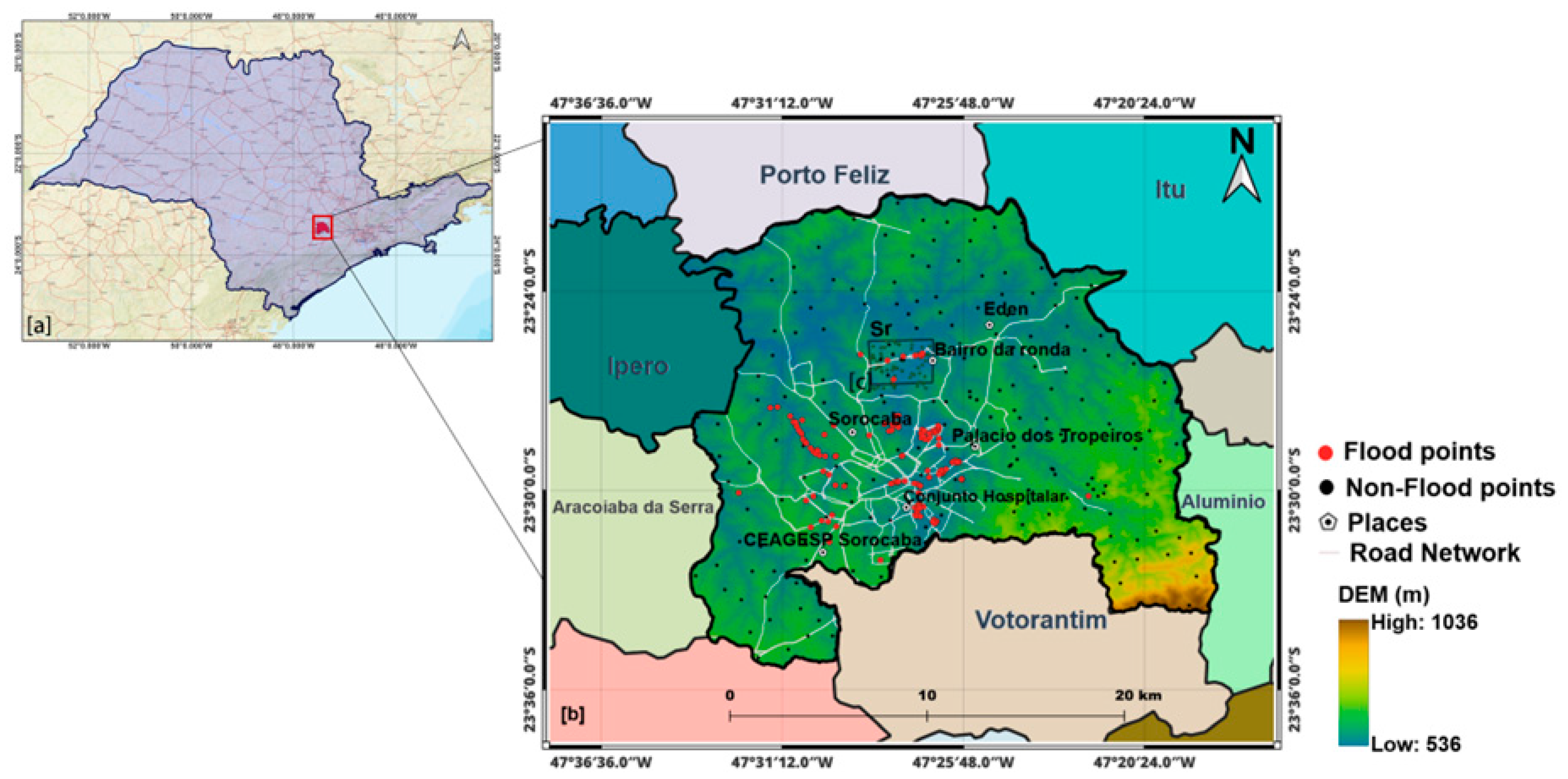
2.1. Study Area

The study area is located in the southeastern region of São Paulo state, 92 km from the capital—São Paulo megalopolis city, Brazil. It lies between latitudes 23°21′ and 23°35′ south and longitudes 47°17′ and 47°36′ west. The municipality of Sorocaba, which encompasses a total area of approximately 450 km2, is the focus of this study. In a typical urban landscape context, 99% of Sorocaba’s inhabitants live in urban areas [36]. The local population was about 723,682 in 2022, ranking it the 7th most populous city in the state [36]. Furthermore, Sorocaba is the headquarters of the Metropolitan Region of Sorocaba, formed by a cluster of 27 cities with a total area of 11,611.48 km2 [37]. Sorocaba, located in the Sorocaba and Médio Tietê sub-basin (UGRHI 10), in Brazil, developed around a river that remains central to the city’s urban landscape. Despite urbanization, the river continues to provide water, support local biodiversity, and serve as a hub for recreational and cultural activities. However, the floodplain of the Sorocaba River has undergone multiple rectification interventions over time, which, combined with its natural susceptibility to flooding, pose significant risks to local communities during the rainy season [38]. The intermittent rainfall started in December 2022 and ended in March 2023. On 12 February 2023 alone, 375 mm of rain fell in the city, with 100 mm falling over six hours—a volume at least 20% higher than the peak in 2017 [39]. The intermittent rainfall in recent years led to severe flooding, as the region experienced an unusually high volume of water within a short timeframe, causing the overflow of the Sorocaba River and its streams [40]. The climate over Sorocaba is classified as Cwa (C = Mild temperate, w = Dry winter, a = Hot summer) by the Köppen system, i.e., subtropical, with dry winters from June to September and rainy summers from December to March. The mean annual temperature is 22 °C, with January and February being the warmest months of the year, and the mean annual precipitation is 1389 mm [41]. From 2015 to 2019, the states in southeastern Brazil experienced 1373 extreme rainfall events (with precipitation above 50 mm/hour), and of these, 730 occurred in São Paulo [42]. The rainfall, combined with intense precipitation events, frequently triggered flash floods and landslides, which account for 70% of natural disasters nationwide and 90% in Southeast Brazil [43]. These events led to the displacement of dozens of families, significant property damage, and loss of life. Due to the climatic and hydrometeorological events described above in flood plains, Sorocaba city has become highly susceptible to flooding during heavy downpours. A subregion (Sr) was isolated in the training area for model validation.

2.2. Geospatial Data

2.2.1. Flood Inventory

Creating a flood inventory map is the first stage in building a machine learning (ML)-based flood susceptibility model. This map shows where previous floods have occurred and how those locations relate to the associated conditioning factors [44]. In our study, the flood inventory from Sorocaba in São Paulo includes 178 reported flood locations distributed across the city, as shown in Figure 1. These were compiled based on reports from the Urban Security Secretariat—Municipal Coordination of Protection and Civil Defense of Sorocaba during the Summer Plan period, which covers December 2022 to March 2023. The data were provided on 10 August 2023, as documented in Administrative Process No. 18468/2023. In addition, field missions were carried out in 2022 before the flood occurrence to detect floodplains by extracting selected remote sensing indices (e.g., NDWI values) from Sentinel-2 satellite images. The essence of this approach is to detect high or low remote sensing index values, which indicate areas that could be flooded during heavy rainfall. A total of 356 samples were acquired to establish the model for Sorocaba, including 178 samples for flood and 178 for non-flood points, respectively. It is important to note that the non-flood samples were generated randomly. In the study by Meliho et al. [45], random points were generated using a single criterion—slope—to filter out non-flooded points. However, our research utilized two criteria for a more accurate selection. Furthermore, we observed that flooded points in our dataset typically have elevation values ranging from 0 to approximately 650 m and normalized difference water index (NDWI) values between 0.23 and 0.98. Consequently, we filtered out non-flooded points in the randomly generated points by including only those with elevations greater than 700 m and NDWI values less than 0.23. In addition, we deployed the synthetic minority oversampling technique (SMOTE) to generate synthetic data samples in addition to the existing data points, increasing the volume of the dataset, balancing it, mitigating bias in the model, and improving the performance of ML models. Flood and non-flood inventory points were labeled 1 and 0, respectively. Flooded and non-flooded locations within the model training area were randomly split into a training set (80%) and a testing set (20%) [34]. Flooded and non-flooded points outside the training area (i.e., Sr) were used to evaluate the ML model transferability.

2.2.2. Flood Driving Factors

In this study, 16 flood-driving factors (FDFs) were considered based on the literature, data accessibility, and watershed characteristics [34,46], prioritizing the inclusion of more influencing variables to make 16 FDFs to enhance prediction accuracy. The identified 16 factors potentially indicate an increased hazard for urban pluvial flooding. These factors represent the topographical (elevation, slope, aspect, total curvature, plan curvature, topographic wetness index (TWI), stream power index (SPI), surface roughness (SR), terrain ruggedness index (TRI), topographic position index (TPI)), anthropogenic (land cover (LC), distance to the river (DTRiver), distance to the road (DTRoad)), and hydrometeorological (moisture, normalized difference vegetation index (NDVI), NDWI) factors. The 10 topographical factors in this study were derived from a digital elevation model (DEM) obtained from the SRTM DEM “https://earthexplorer.usgs.gov (accessed on 6 January 2025)” at a spatial resolution of 30 m. The hydrometeorological factors and LC were obtained from high-resolution Level-2 Sentinel-2 cloud-free optical satellite imagery with a spatial resolution of 10 m downloaded from “https://apps.sentinel-hub.com/eo-browser (accessed on 6 January 2025)”. As for DTRiver, the river topology shapefile was obtained from HydroRIVERS “https://www.hydrosheds.org/products/hydrorivers (accessed on 7 July 2024)”, which is a vectorized line network of all rivers with a catchment area of at least 10 km2, an average river flow of at least 0.1 m3/s, or both [47]. This dataset has been widely used in flood susceptibility and hydrological studies to analyze river networks and their impact on flooding [48]. This dataset extracted major rivers in Sorocaba, and the distance to the river (DTRiver) was calculated and analyzed to assess flood susceptibility. Distance from each flood and non-flood point to the nearest road was calculated using GIS-based spatial analysis, leveraging OpenStreetMap (OSM) standard maps to evaluate infrastructure vulnerability and accessibility during flooding events [49]. Finally, each FDF was transformed into a raster format using QGIS.
Elevation is one of the most essential flooding-triggering factors. Higher elevations generally experience less flooding as water flows downhill naturally due to gravity. Conversely, low-lying areas are prone to water accumulation and flooding, particularly during heavy rainfall or river overflow [50].
Slope is the most vital driving factor because it affects flow velocity and water accumulation capacity. For instance, steeper slopes result in faster water runoff, reducing the likelihood of flooding locally but increasing downstream flood risk. Gentle slopes allow water to pool, elevating flood risk in flat regions [51]. In this study, we consider the slope measurement to be a fixed variable since the region under investigation involves remote sensing-based flood mapping, where slope is commonly used to distinguish flooded low-lying areas from higher elevations
Aspect indicates the direction of the maximum slope. The direction a slope faces significantly affects flooding, as it impacts the local climate patterns, infiltration, and soil moisture [52].
Total curvature defines the shape of the land surface. Convex areas shed water efficiently, reducing flood risk, whereas concave areas accumulate water, making them more flood prone [53].
Plan Curvature describes land curvature in the horizontal plane. Concave plan curvature channels water flow into depressions, increasing flood susceptibility, while convex curvature disperses water and reduces flood risk [54].
TWI is a physical property that measures potential water accumulation and is calculated using slope and upstream contributing area. Higher TWI values indicate regions likely to retain water and experience flooding [55]. It is calculated as TWI = ln (As/tanβ), where ‘As’ is the specific watershed area (m) and ‘β’ is the slope gradient (°) [8].
SPI quantifies the erosive energy of flowing water based on slope and discharge. Areas with high SPI values are prone to erosion and flooding, particularly in steep terrains with high water flow [56].
SR is a property that slows down water flow, potentially lowering peak flood levels but prolonging flooding duration. Rough surfaces also encourage water infiltration, reducing runoff volume [57].
TRI measures elevation variability. Rugged terrains create barriers to water flow, causing localized flooding in valleys and low-lying areas [58].
TPI is a property that compares the elevation of a point to its surroundings. Negative TPI values (valleys) are more prone to flooding, while positive TPI values (ridges) are less susceptible [59].
LC significantly influences flooding by affecting water absorption, storage, and transport, with impervious surfaces increasing runoff, vegetation enhancing infiltration, agricultural practices varying in impact, and wetlands mitigating flood risk [60]. However, LC has different water impermeability depending on the land use.
DTRiver is essential because geographical areas closest to the river often experience the most significant flood inundation [61]. This means that the farther a residential area is from the river, the lower its flood susceptibility.
DTRoad is another significant factor in flood susceptibility mapping, as it measures the Euclidean distance from a specific point to the nearest road. In urban areas, the limited capacity of stormwater drainage systems can cause runoff to travel along roads, which can then become preferential pathways for water flow during pluvial flooding [62].

3. Model Feature Importance (MFI) and ML Models

This section summarizes the importance of feature dependency frameworks (FDFs) in model development, specifically in model feature importance (MFI). MFI is a machine learning technique used to assess the significance of each input feature in predicting the target variable. It helps identify which features most significantly influence the model’s predictions. Understanding feature selection and its importance is a crucial step that must always be addressed before developing a model. Figure 2 presents a heatmap, which serves as a visual representation of the correlation matrix. The color coding in the heatmap denotes the correlation values between features, highlighting patterns within the matrix and indicating which variables are most strongly correlated. Furthermore, it alerts us to potential multicollinearity issues, where two or more variables show high correlations. Datasets affected by multicollinearity can complicate the development of machine learning models, leading to inaccuracies in flood susceptibility models and misrepresenting significant variables [63]. In Figure 2, multicollinearity issues are evident, as more than four features (land cover (LC), normalized difference water index (NDWI), normalized difference vegetation index (NDVI), DTRiver, etc.) demonstrate strong correlations, which are indicated by the blue-bordered boxes.
However, the variance inflation factor (VIF) has often been reported as an effective measure for addressing multicollinearity challenges in model development. It helps to eliminate correlated features, thereby ensuring the stability and interpretability of coefficients, enhancing the model’s generalizability. This method is commonly employed in flood risk assessment studies and flood susceptibility modeling [46,64]. However, there are still limitations and challenges associated with using VIF for such modeling, as it only assures statistical rigor in regression models, particularly when multicollinearity is a concern, but does not impact model accuracy. Hence, here, we utilize recursive feature elimination.

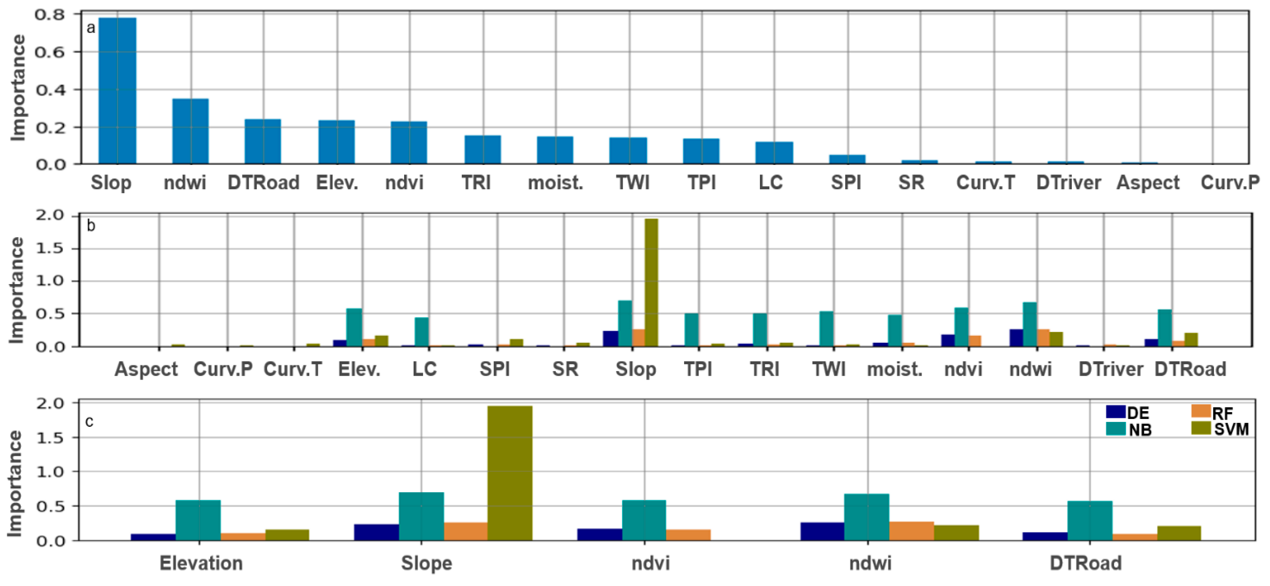
3.1. Recursive Feature Elimination (RFE)

RFE is generally considered a more effective method than VIF for improving model performance and predictive power. It achieves this by eliminating noise and redundancy or discarding highly correlated and less important features, reducing multicollinearity through an iterative process, thereby improving model accuracy. In contrast, VIF solely focuses on identifying and quantifying multicollinearity by identifying coefficient instability, which does not necessarily lead to enhanced predictive performance. RFE surpasses VIF in predictive tasks, particularly when addressing model-driven feature selection, non-linear relationships among features, and the direct impact of features on the model [65,66]. Algorithm 1 describes the RFE algorithm in pseudocode with bars for routines and tabulation. It outlines the step-by-step procedure used in this study for feature selection in ML to identify the most significant features in a dataset.
Algorithm 1. RFE Algorithm in Pseudocode with Bars for Routines and Tabulation.
Input:
   X—Feature matrix (n_samples x n_features)
   Y—Target vector
   model: Machine learning Model with feature importance
   k: Desired number of features to select
Initialize:
   X_remaining ← X           // Start with the full dataset 
   feature_set ← All feature indices
while len (X_remaining) > k:        // Continue until k features remain 
   Train Phase:
     Model.fit (X_remaining, y)
   Ranking Phase:
     importance_scores ← model.feature_importances_
     ranked_features ← argsort (importance_scores)
   Elimination Phase:
     least_important ← ranked_features [0]
     feature_set ← feature_set \ {least_important}
     X_remaining ← X [:, feature_set]
Output:
   X_remaining—Feature matrix with top k features

3.2. Methodology Flowchart and Models

This subsection briefly describes the different model types of methodology and setups, including hyperparameters for FSM. This study typically follows a systematic flowchart, as shown in Figure 3. It starts with 16 variable extractions from data sources described in Section 2.2.1, preprocessing (data cleaning, normalization, and feature selection), model training, validation, and result interpretation. Various ML algorithms were deployed in developing the ML models, namely, random forest, support vector machines, differential evolution, and naïve Bayes.

3.2.1. Random Forest (RF) Model

The RF algorithm [67] is a powerful robust machine learning (ML) algorithm commonly used for multi-class classification, regression problems, and predictive modeling. It proved optimal for our study due to its efficiency in addressing highly complex and nonlinear relationships between input variables. It has been widely applied in various fields, including FSM [34,68]. The algorithm operates by building multiple decision trees, each trained on different subsets of data. Let yi represent the prediction output for an input X from a decision tree, where X might include input features like elevation, slope, LC, etc., where each tree provides a prediction, denoted as yi, and the final predicted value Y is obtained by averaging the predictions from all the trees. Y is calculated as follows:
  y i = T i   ( X )
Y = 1 n   i = i n ( y i )
where yi is the predicted value from the i-th individual decision tree, Ti is the i-th decision tree, Y is the final predicted value from the RF model, and n is the total number of decision trees in the forest. For classification problems, RF output Y is determined by majority voting:
Y = m o d e { T 1 X , T 2 X ,   T 3 X , . ,   T N X }        
where “mode” indicates the most frequently predicted class among the trees.

3.2.2. Support Vector Machine (SVM) Model

SVMs have proven effective in predicting floods because they can manage complex, nonlinear relationships among environmental variables. SVMs employ a kernel function to transform input features obtained from the RFE method used in this study into higher-dimensional spaces. This transformation allows for the classification of flood-prone areas. One of the key advantages of SVMs is their robustness against overfitting, particularly when working with high-dimensional datasets, making them a preferred choice in hydrology and flood risk assessment studies [69]. SVMs use a hyperplane to separate data into distinct classes or predict continuous values, making them suitable for both classifications (e.g., flood/no-flood). It has been applied in diverse contexts, including flood susceptibility mapping, and real-time flood forecasting, providing accurate and scalable predictions to support disaster management efforts [70]. The robustness of SVMs in managing high-dimensional and noisy datasets makes them a popular choice for flood susceptibility analysis [71]. SVMs are mathematically represented as:
Y x = s i g n   i = 1 n a i y i K X ,   X i + b
where X is the input features, Xi are the support vectors (critical data points), yi are labels of support vectors (e.g., flood/no-flood), K (X, Xi) is the kernel function used to map inputs into higher-dimensional space (i.e., linear, polynomial, radial basis function), ai are Lagrange multipliers, representing the importance of support vectors, while b is the bias term.

3.2.3. Differential Evolution (DE) Model

DE is an optimization algorithm designed to solve complex problems by iteratively refining candidate solutions. This biologically inspired algorithm was introduced by Storn and Price [72]. DE has been applied to estimate the parameters of hydrological models, enhancing the accuracy of flood frequency analysis and prediction, as noted by Yilmaz et al. [73]. Further details about the application of DE can be found in the work of Zhang et al. [74].

3.2.4. Naïve Bayes (NB) Model

Naïve Bayes (NB) is a probabilistic ML algorithm based on Bayes’ theorem, assuming independence between input features. The NB classifier effectively argues that the presence of one feature within a class does not depend on the existence of any other feature. This independence assumption allows for efficient and robust classification, making it a reliable tool in various applications. Its application in flood prediction includes susceptibility mapping, early warning systems, and decision support for flood risk management [75]. The model predicts the most probable outcome (flood or no flood) by maximizing posterior probabilities. For a given set of features, P c x 1   , x 2   ,   x 3   ,   ,   x n   ) from P c ,   P x 1   , x 2   ,   x 3   ,   . ,   x n , and P ( x 1   , x 2   ,   x 3   ,   . ,   x n   | c ) [76]. The NB is mathematically represented as:
P c x 1   , x 2   ,   x 3   ,   ,   x n   ) = P x 1   , x 2   ,   x 3   ,   ,   x n   c     P c   P x 1   , x 2   ,   x 3   ,   ,   x n  
P x 1   , x 2   ,   x 3   ,   ,   x n   c = i = 1 n P x i   c = P x 1   c     P x 2   c     P x 3   c     P x n   c
where P c x 1   , x 2   ,   x 3   ,   ,   x n ) is the posterior probability of class (c, target) given features x i   (where x i   are the features), P ( c ) is the prior probability of class c (likelihood of flood without knowing the features), P x 1   , x 2   ,   x 3   ,   ,   x n   | c is the likelihood of a feature x i   given class c, and P x 1   , x 2 ,   x 3   ,   ,   x n is the evidence or normalization factor (sum of probabilities for all classes).
The model predicts the class c that maximizes P c x ) :
c = arg m a x c   P c i = 1 n P x i   c
where P(C) is the prior probabilities for flood and no-flood scenarios and P x i   c is the likelihood of each feature being based on the training data.

3.3. Model Explainability and Feature Importance

Previous flood studies in São Paulo have not examined the significance of individual factors in predicting pluvial flood susceptibility. In this study, we employed the explainable artificial intelligence (XAI) technique known as Shapley additive explanations (SHAP) to identify the key elements influencing the predictions made by our machine learning model when assessing flood susceptibility and their effects on individual outcomes. Utilizing the SHAP Python package (version 3.8), we assign an importance value to each feature for each prediction [77]. This method is particularly beneficial for evaluating flood susceptibility, as it also indicates whether a feature has a positive or negative impact on the projected results [34,46,78].

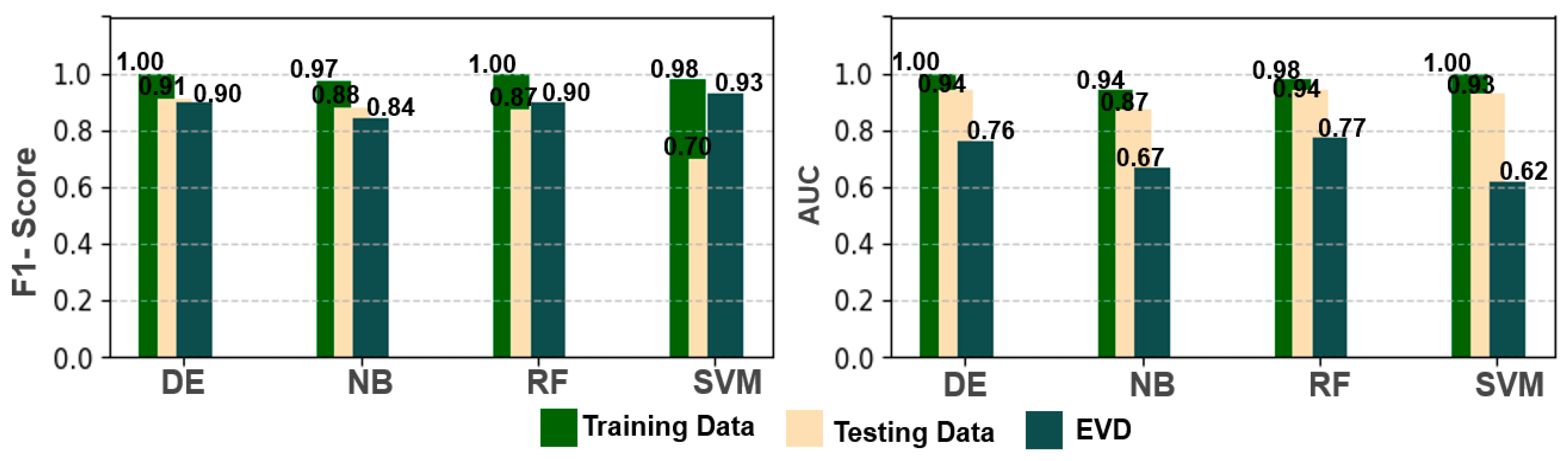
Model Performance Metrics

This study used statistical indices such as the F1-score and the area under the curve (AUC) to assess model performance. We considered our dataset to be relatively small compared to those used by Seleem et al. [34] and Kurugama et al. [46]. Therefore, we decided to refrain from using the Kappa statistic, which could lead to unreliable and unstable estimates [79]. The F1-score and AUC are commonly employed evaluation metrics in flood susceptibility and geohazard modeling studies [46,78] because they provide robust insights into model performance, particularly under conditions of class imbalance, which is frequent in geospatial hazard datasets. The maximum F1-score is 1, which indicates perfect accuracy and recall, while the minimum is 0, occurring when both precision and recall are zero. AUC values range from 0 to 1, where 1 represents an ideal model and 0.5 signifies performance on par with random predictions [34,64]. Understanding this scale is essential for evaluating and improving model effectiveness. The calculations for AUC and F1 scores are outlined below:
A U C = T P + T N   P + N ,   F 1 s c o r e = 2 T P   2 T P + F P + F N
where TP, TN, FP, and FN are true positives, true negatives, false positives, and false negatives, respectively. P denotes the presence of floods, while N indicates their absence.

4. Results and Discussion

4.1. RFE as an Anti-Multicollinearity

RFE is a preprocessing technique used in this study to mitigate the effects of multicollinearity, particularly because machine learning models are sensitive to correlations between features. This technique helps in removing redundant or less important features. As a result, RFE did not consider all 16 FDFs in the feature importance analysis during the development of the flood model. Figure 4a–c display bar charts illustrating the significance of feature importance across the machine learning models. Despite considering 16 features in this study, the bar chart in Figure 4b shows that RFE directly evaluates only the importance of the 10, 10, 12, and 12 features that are relevant for the NB, SVM, RF, and DE models, respectively.
All bar plots in Figure 4a–c exhibit significance of feature importance for the models. It is evident from the charts that every model exhibits a different preference for their significant feature. The NB model exhibits the highest number of features that were considered, followed by the DE model, while the RF model and the SVM model considered the least number of features. In all the categories of Figure 4, slope exhibits the highest significant feature, while the curvature plan exhibits the lowest value of feature importance. In addition, the topographical and hydrometeorological categories are the prominent factors driving the flood as observed in Figure 4.

4.2. Model Performance Comparison and Validation

We used 16 factors potentially affecting flood susceptibility as training data to create flood susceptibility maps for Sorocaba with several data-driven algorithms. Flood susceptibility levels vary from 0 (the lowest) to 1 (the highest). We categorized the visualization of the flood occurrence probability values into five susceptibility classes: very low, low, moderate, high, and very high [80]. In addition, we produced a flood susceptibility map for the sub-region within Sorocaba that exhibits topographic depressions Sr (Figure 1) outside the training area, which we regarded as external validation data (EVD). The primary essence of our model validation was to improve accuracy and minimize overfitting during the model-training process, evaluate how well the model performs, and test the model’s robustness and most importantly, model transferability. Hence, the test dataset and EVD were utilized for this purpose. The optimal hyperparameters for each classification model were determined using the “Grid Search” algorithm. The grid search algorithm was implemented in our Python-based machine learning pipeline using GridSearchCV from scikit-learn to systematically optimize hyperparameters. The hyperparameters tuning process was dynamically adapted to the dataset characteristics and the performance of different ML models. Grid search exhaustively evaluates all possible combinations of specified hyperparameter values through cross-validation. Although this approach is computationally intensive, it ensures robust model selection, minimizing overfitting and enhancing generalization. As hyperparameter requirements vary across algorithms, there are many we considered depending on the specific algorithm. However, we have highlighted a few critical hyperparameters for performance optimization. These include “n_estimators,” “max_depth,” “min_samples_split,” “max_features,” and “learning_rate”. All these, among others, were some of the key hyperparameters implemented in our ML pipeline for this study. We evaluated DE, NB, RF, and SVM model performance based on the F1-score and AUC metrics. Figure 5 illustrates the accuracy results for the model training set, testing set, and the points outside the training dataset, which we regarded as external validation data (EVD). Based on the F1-scores and AUC values across all models, both the training and testing datasets demonstrated strong performance, with all metrics exceeding 0.7.
These results indicate the models’ high capability to distinguish between flooded and non-flooded areas based on feature importance. Notably, the AUC values for the testing dataset were particularly impressive, ranging from 0.87 to 0.98, while F1-scores varied from 0.70 to 0.91 across all models. The model transferability analysis using the EVD revealed F1-scores between 0.84 and 0.93, with AUC values ranging from 0.62 to 0.77. Among all models, the DE model consistently outperformed the others in training and testing datasets for F1-scores and AUC values. In contrast, the SVM model achieved the highest F1-score during the EVD analysis but demonstrated lower overall performance than the DE model. A comprehensive assessment across the training, testing, and external datasets showed variations in the models’ sensitivity and effectiveness in predicting flooded and non-flooded regions. The DE model achieved a perfect score of 1.00 for both F1-score and AUC metrics, followed by the RF, NB, and SVM models, as shown in Figure 5. However, the NB and SVM models exhibited relatively lower performance during the EVD analysis, with AUC values between 0.62 and 0.67, indicating moderate differentiation capability. Metrics above 0.75 suggest strong predictive performance, while those between 0.62 and 0.67, although exceeding the random guessing threshold of 0.50, highlight areas for improvement. Increasing the volume or diversity of data may further enhance these results. The performance levels are currently acceptable, but ongoing efforts will focus on optimizing these models. Overall, the EVD analysis confirms that the models demonstrate good and moderate predictive performance for regions outside the training area, as reflected in the F1-scores and AUC evaluations.

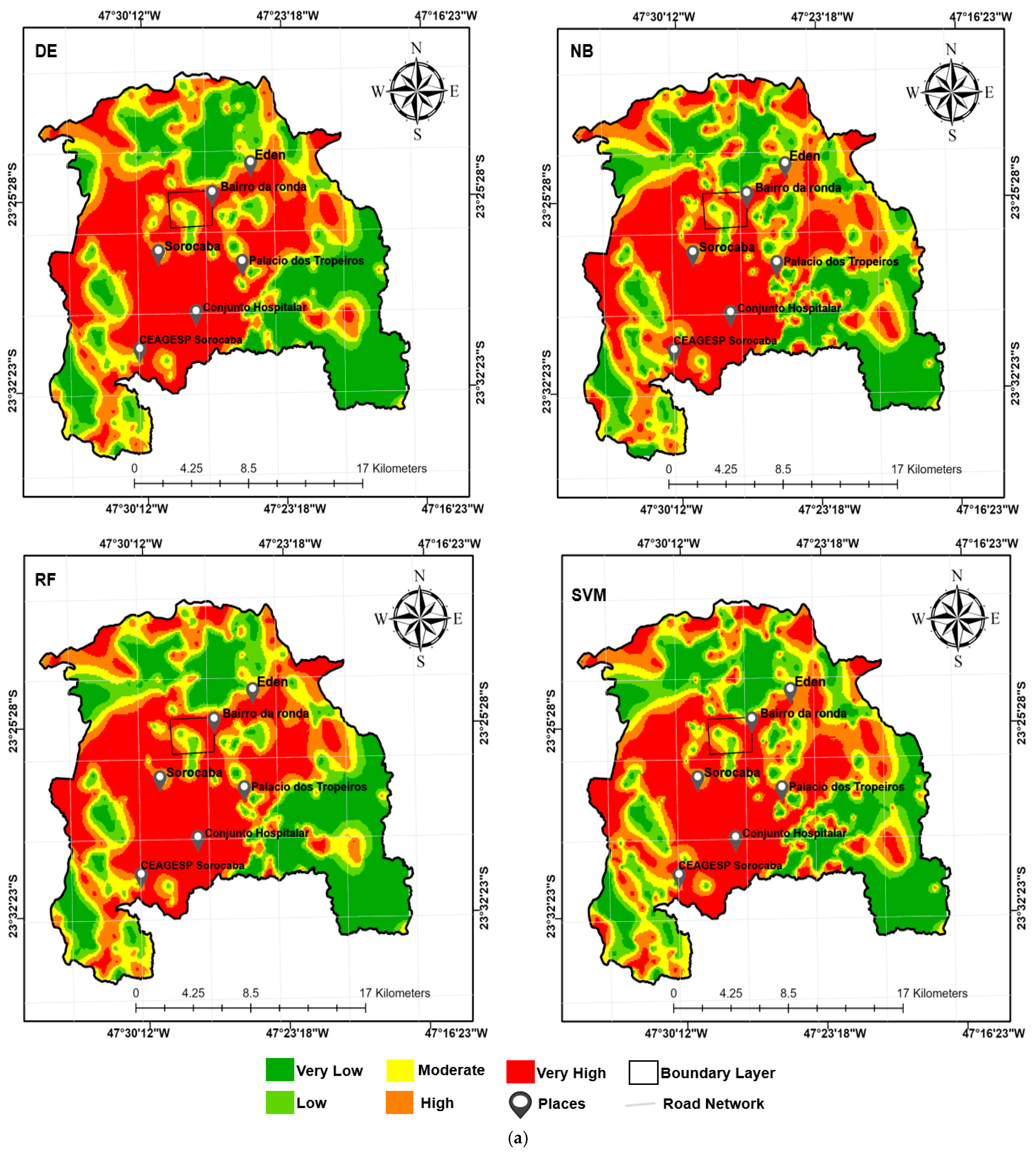
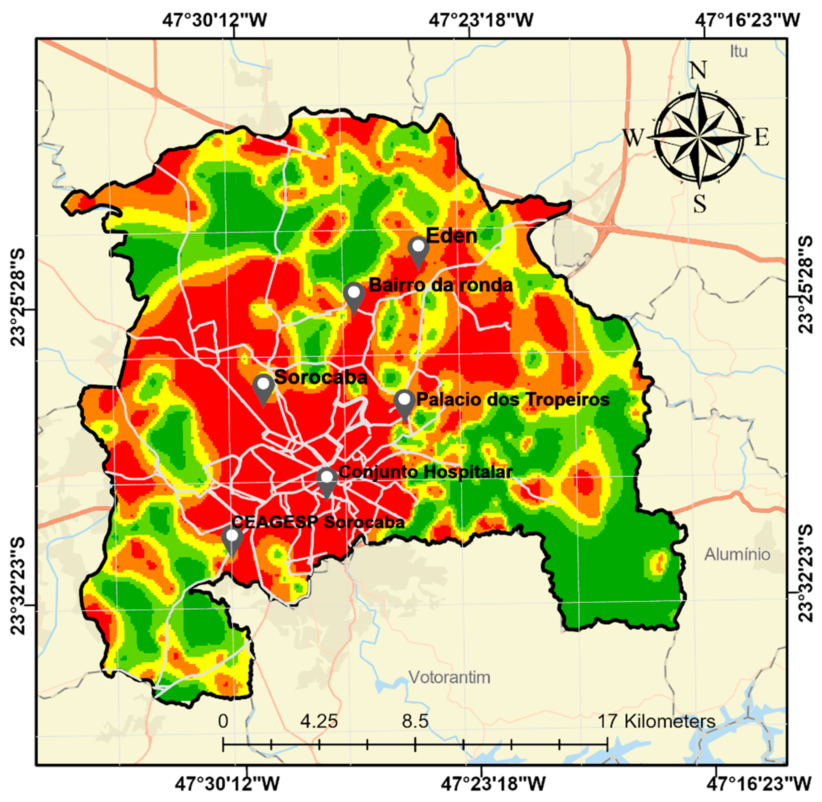
4.3. Flood Model Susceptibility in São Paulo Sub-Region

Flood susceptibility maps were created for Sorocaba, a sub-region of São Paulo, Brazil, using the four different models, as illustrated in Figure 6a. We mapped the flood susceptibility and calculated the probability of flooding utilizing the machine learning function syntax ‘predict proba’ in the Python programming platform. This function returns a list of arrays, where each array contains two values: one representing the probability of not being flooded, and the other indicating the likelihood of being flooded. All models suggest that the southwestern part of Sorocaba predominantly consists of watersheds due to its topographic features, making this area highly vulnerable to flooding. In contrast, the northern parts of Sorocaba show lower vulnerability. The low-lying areas most prone to flooding are characterized by gentle slopes and low elevation.
Conversely, areas farther from the river demonstrate reduced vulnerability, as Figure 4a,b confirm. Overall, the likelihood of flooding increases as the distance to the river decreases and elevation lowers. Following the approach of Meliho et al. [45], Figure 6a displays the flood susceptibility map. The susceptibility maps are classified into five categories: very low (0–0.2), low (0.2–0.4), moderate (0.4–0.6), high (0.6–0.8), and very high (0.8–1.0). We further computed the percentage quantification of flood over Sorocaba, which we classified as the summation of the flood zones and flood susceptible zones for all models as shown in Figure 6b.
Despite the good performance of the models discussed in Section 4.2, it is still essential to compare the results of the different models (DE, NB, RF, and SVM) to identify areas of most common agreement. Hence, we generated the final flood susceptibility map as shown in Figure 7, where we integrated the predominant spatial predictions and classifications derived from the four models, emphasizing areas of consensus. It is important to note that we computed mean values at spatial locations with minor variations or no consensus predominant spatial predictions, rather than confidently assigning them to low or high flood risk categories. However, such areas with prediction variations are minimal. Careful visual observation reveals that the predicted flood susceptibility areas within the bounding box (i.e., Sr) in Figure 6a vary across different models. Additionally, most of the flood points identified in Figure 1 within the “Sr” region correspond to predicted flood susceptibility zones, ranging from moderate to very high, as shown in Figure 6a. This study underscores the significance of model transferability, particularly as demonstrated in the “Sr” region. This capability enables the prediction of flood susceptibility in areas beyond the model’s training region.
Enhancing this approach could involve incorporating additional training data or applying transfer learning techniques [81]. Future research should further investigate model transferability, especially in urban environments. Additionally, as observed in Figure 7, all models demonstrate that the impact of the road network on identifying locations with high flood susceptibility is particularly pronounced in the Sorocaba region, especially in residential zones. We analyzed the watershed drivers in Sorocaba by focusing on five key characteristics of areas with metric values (extracted from the GIS platform): low elevation, high moisture levels, low land cover, low slope, and high TWI (i.e., indicates areas prone to water accumulation). Understanding these factors is crucial for assessing drainage and hydrological processes.
Our analysis suggests that the central and southwestern regions of Sorocaba are highly vulnerable to flooding, a conclusion supported by our models, as illustrated in Figure 6 and Figure 7. Spatial locations with susceptible prediction variations in categories as described earlier could be due to inherent uncertainties in the ML modeling process, but they can be minimized, managed, and quantified. These uncertainties in our findings may arise from the different ML algorithms or model usage perspectives to simplify and represent complex environmental variables, as well as varying assumptions and data handling approaches. Overall, these findings serve as a valuable resource for decision-makers seeking to implement measures to mitigate flood risk in São Paulo and its surrounding region. Contrary to the findings by Meliho et al. [45] and Seleem et al. [34], who reported that KNN and RF models, and RF and SVM models, respectively, performed better than others in their study, our research shows that DE and RF models outperformed the other models including SVM in some specific scenarios. This suggests that ML algorithms and architecture responses to model performance can vary based on the criteria established for model development. This study has demonstrated the major significance of model transferability, as exhibited in “Sr” in Figure 6a, which enables the prediction of flood susceptibility for areas outside the model’s training area. The approach could be improved by incorporating additional training data or implementing transfer learning techniques [81]. Future studies require more testing of model transferability, especially in urban areas.

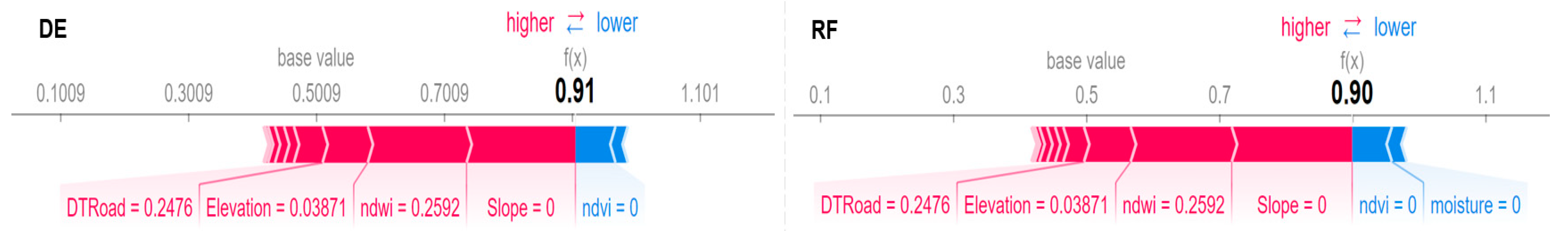
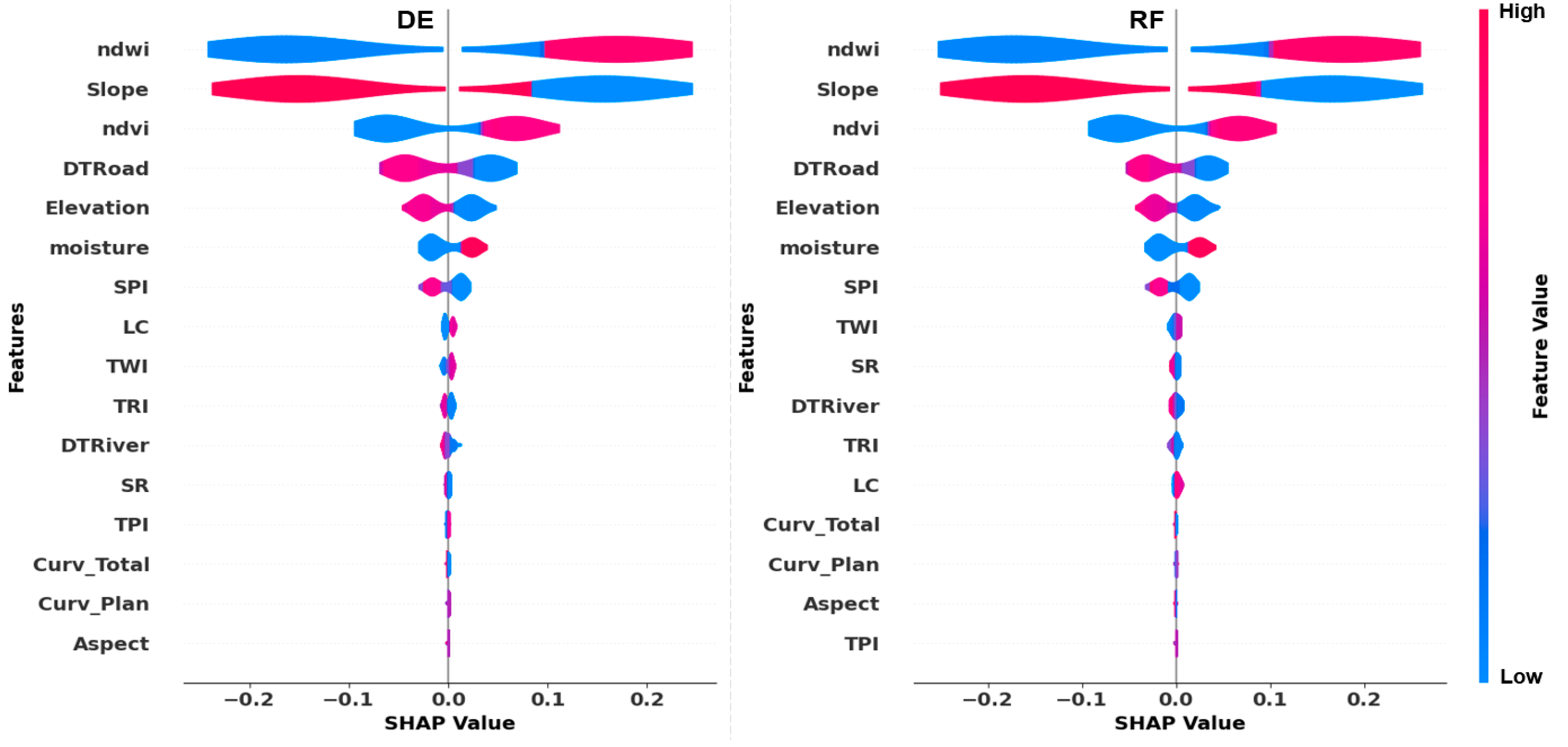
4.4. Model Feature Importance Assessment

In this study, we utilize the Shapley additive explanations (SHAP) technique as a post-modeling tool to analyze the importance of various features in model predictions. This technique distributes the model’s output among different features based on their contributions, providing a comprehensive understanding of their influence after training. The SHAP summary plot ranks the features according to the total magnitudes of their SHAP values across all samples. It illustrates the distribution of each feature’s impact on the model’s output. Our analysis focuses explicitly on DE and RF, as these consistently outperformed other models across all three dataset categories—training, testing, and external datasets. The SHAP results highlight the significance of each feature in the predictions, with red indicating a positive contribution to the model score and blue indicating a negative contribution. These results indicate whether a feature increases or decreases the probability of a given class (flooded or non-flooded), thereby influencing the predicted values. For example, Figure 8 shows the flood susceptibility levels of 0.91 and 0.90 for a specific location in Sorocaba, as determined by the DE and RF models, respectively.
The SHAP values were derived by analyzing the cumulative contributions of all FDFs to the baseline probability, which is approximately 0.50 for both models. The highlighted scores of 0.91 and 0.90 indicate the DE and RF models’ predictions for this observation. Higher scores correspond to a prediction of 1.0 (flooded), while lower scores indicate a prediction of 0 (not flooded). Features that significantly impacted the score are positioned closer to the boundary between red and blue, with the size of the bar representing the extent of that influence. As a result, these points were classified as flooded, as they were influenced upward by all the factors indicated in red. Figure 9 illustrates the SHAP summary plot, which shows the maximum, average, and minimum values for each feature across all samples in the testing dataset. The distribution of red and blue violin bars offers insights into how each feature impacts model predictions concerning flooding. The results indicate that predictor variables influence whether an area is classified as flooded or non-flooded based on specific site characteristics.
Floods are more likely to occur in regions with high NDWI values, particularly near steep slopes and high NDVI values. Additionally, shorter distances to roads (DTRoad) and lower elevations increase the susceptibility to flooding. The absolute SHAP values indicate the significance of each feature in the model’s prediction process. According to the SHAP analysis, the top seven features influencing flood occurrence are NDWI, slope, NDVI, DTRoad, elevation, moisture, and SPI. This finding is consistent with Figure 4, which supports the results of the RF model. Meanwhile, variables such as TWI, distance to rivers (DTRiver), TRI, and land cover (LC) moderately influence both models. Other features, including total and plan curvature, TPI, and aspect, show a relatively lower impact on flood occurrence. The response of the SR feature varies between the DE and RF models. Notably, moisture and land cover features are widely recognized for their critical roles in hydrological models. The SHAP analysis confirms their differing levels of importance in the RF model, which range from high to moderate. These findings align well with the findings of Chen et al. [82], who reported that moisture levels significantly influence key hydrological processes, such as infiltration and runoff. At the same time, land cover affects water absorption, storage, and transport across landscapes. Consequently, these factors significantly impact the accuracy and reliability of hydrological predictions [82].

5. Conclusions

Floods are among the most destructive natural hazards globally. This study utilized four ML algorithms—DE, NB, RF, and SVM—to develop flood prediction susceptibility models specifically for Sorocaba. Sixteen predictor variables (i.e., FDFs) were analyzed. The performance of these models was compared in terms of their ability to map flood susceptibility. The study highlights how the dynamics of these predictor variables interact with different ML algorithms and architectures, emphasizing their impact across various ML frameworks. The findings indicate that topographical, anthropogenic, and hydrometeorological factors play significant roles in predicting flood occurrences. Notably, elevation, slope, NDVI, NDWI, and distance to roads emerged as the top five influential FDFs in flood susceptibility mapping for Sorocaba. Based on the performance metrics—F1-score and AUC scores—it is clear that all models exhibited strong performance during both the training and testing phases, with scores ranging from 0.94 to 1.00. Ultimately, the DE model is the top performer, as it emerges as the most robust and reliable choice for predicting flooded and non-flooded areas, given its perfect F1-score and AUC metrics of 1.00 in both training and testing datasets in this study. Models such as RF or SVM may require an iterative evaluation process using a larger dataset to account for potential variability in performance. Interestingly, both the DE model and the RF model outperformed the others across all three stages: training, testing, and evaluation on an external dataset. The SVM model demonstrates the highest F1-score (0.93), when considering external validation data (EVD), albeit with lower overall performance compared to DE. The RF model performs consistently well across all datasets, while DE occasionally outperforms RF and SVM in specific scenarios. While RF exhibits slightly better AUC values than SVM in EVD, this does not necessarily establish RF as the superior model. Instead, it highlights the need for further testing across diverse datasets and scenarios, or a large dataset to determine whether these variations are consistent or context-dependent. This hypothesis may be subject to further analysis in our future study.
This study also explores the concept of model transferability, assessing the potential for flood susceptibility predictions in regions outside the model’s training area. The results demonstrate that this method can be effectively applied to other parts of the country, providing an efficient approach to generating flood susceptibility maps, especially in data-scarce regions. Our results indicate that all models displayed moderate–good performance, as shown in Figure 5. The percentage quantification of flood-susceptible zones, illustrated in Figure 6b, reveals that approximately 41% to ~50% of areas in the Sorocaba sub-region could be at very high risk of flooding. According to the SHAP analysis, the predominant distribution of these high-risk zones is primarily characterized by factors such as NDWI, slope, NDVI, distance to roads, elevation, moisture, and SPI. Furthermore, this study demonstrates the potential application of the model in guiding policymakers and decision-makers in developing targeted flood mitigation strategies, land-use planning, and improving infrastructure resilience. However, while the model effectively identifies flood-prone areas, it also has limitations. Notably, the study does not explicitly account for hydrodynamic parameters such as flood depth, velocity, and frequency—essential for comprehensive flood analysis. These parameters typically require the integration of hydrological models (e.g., HEC-HMS, SWAT) and hydraulic models (e.g., HEC-RAS 2D), which although falls outside the scope of this study. While we experience a seemingly good performance of the ML models tested on EVD, this may be attributed to the fact that the external geographical area where the EVD was obtained may have comparable geomorphological and environmental settings to Sorocaba. Our future research will focus on the development of a hybrid modeling framework that integrates physically based hydrological and hydraulic models with ML techniques. Such an approach aims to improve model generalizability, enable broader applicability regardless of underlying soil or geomorphological conditions, and enhance predictive accuracy.

Author Contributions

Conceptualization, T.S.O. and D.C.; methodology, T.S.O.; validation and formal analysis, T.S.O., M.P.R., D.C., M.B.A., S.H.T. and A.E.D.; investigation, T.S.O.; data curation, T.S.O. and M.B.A. writing—original draft preparation, T.S.O.; writing—review and editing, all authors; supervision, D.C. All authors have read and agreed to the published version of the manuscript.

Funding

This research was funded by the office of the Vice-Principal Research (VPR) Fund of Queen’s University, ON, Canada, and the Natural Sciences and Engineering Research Council of Canada (NSERC) Discovery Grant.

Data Availability Statement

Data are available in a publicly accessible repository at https://apps.sentinel-hub.com/eo-browser (accessed on 6 January 2025).

Acknowledgments

The authors thank the Sentinel satellite data hub for making the satellite optical data available through the EO web browser. We also thank Marina Pannunzio Ribeiro who made data available from the Urban Security Secretariat—Municipal Coordination of Protection and Civil Defense of Sorocaba, São Paulo province.

Conflicts of Interest

The authors declare no conflicts of interest.

References

  1. UNDRR. The Human Cost of Disasters: An Overview of the Last 20 Years (2000–2019); United Nations Office for Disaster Risk Reduction: Geneva, Switzerland, 2020; pp. 13–17. Available online: https://www.undrr.org/publication/human-cost-disasters-overview-last-20-years-2000-2019 (accessed on 1 November 2024).
  2. Doocy, S.; Daniels, A.; Packer, C.; Dick, A.; Kirsch, T.D. The Human Impact of Earthquakes: A Historical Review of Events 1980–2009 and Systematic Literature Review. PLoS Curr. 2013, 5, e50bb9494b3c1. [Google Scholar] [CrossRef] [PubMed]
  3. Opolot, E. Application of Remote Sensing and Geographical Information Systems in Flood Management: A Review. Res. J. Appl. Sci. Eng. Technol. 2013, 6, 1884–1894. [Google Scholar] [CrossRef]
  4. CRED; UNDRR. Economic Losses, Poverty, and Disasters (1998–2017); Centre for Research on the Epidemiology of Disasters and United Nations Office for Disaster Risk Reduction: Brussels, Belgium, 2018; pp. 8–13. Available online: https://www.undrr.org/publication/economic-losses-poverty-disasters-1998-2017 (accessed on 1 November 2024).
  5. Kundzewicz, Z.W.; Kanae, S.; Seneviratne, S.I.; Handmer, J.; Nicholls, N.; Peduzzi, P.; Mechler, R.; Bouwer, L.M.; Arnell, N.; Mach, K.; et al. Flood Risk and Climate Change: Global and Regional Perspectives. Hydrol. Sci. J. 2014, 59, 1–28. [Google Scholar] [CrossRef]
  6. IPCC. Climate Change 2021: The Physical Science Basis; Intergovernmental Panel on Climate Change: Geneva, Switzerland, 2021; Available online: https://inthistogetheramerica.org/2021/08/11/the-ipcc-report-and-what-it-means (accessed on 1 January 2023).
  7. Bradshaw, C.J.A.; Sodhi, N.S.; Peh, K.S.H.; Brook, B.W. Global evidence that deforestation amplifies flood risk and severity in the developing world. Glob. Change Biol. 2007, 13, 2379–2395. [Google Scholar] [CrossRef]
  8. Khosravi, K.; Shahabi, H.; Pham, B.T.; Adamowski, J.; Shirzadi, A.; Pradhan, B.; Dou, J.; Ly, H.-B.; Gróf, G.; Ho, H.L. A Comparative Assessment of Flood Susceptibility Modeling Using Multi-Criteria Decision-Making Analysis and Machine Learning Methods. J. Hydrol. 2019, 573, 311–323. [Google Scholar] [CrossRef]
  9. Beven, K.J. Rainfall-Runoff Modelling: The Primer; Wiley-Blackwell: Hoboken, NJ, USA, 2012; pp. 1–456. [Google Scholar] [CrossRef]
  10. Abdullah, M.F.; Siraj, S.; Hodgett, R.E. An Overview of Multi-Criteria Decision Analysis (MCDA) Application in Managing Water-Related Disaster Events: Analyzing 20 Years of Literature for Flood and Drought Events. Water 2021, 13, 1358. [Google Scholar] [CrossRef]
  11. Mendoza, G.A.; Martins, H. Multi-criteria decision analysis in natural resource management: A critical review of methods and new modelling paradigms. For. Ecol. Manag. 2006, 230, 1–22. [Google Scholar] [CrossRef]
  12. Seleem, O.; Heistermann, M.; Bronstert, A. Efficient Hazard Assessment for Pluvial Floods in Urban Environments: A Benchmarking Case Study for the City of Berlin, Germany. Water 2021, 13, 2476. [Google Scholar] [CrossRef]
  13. Petroselli, A. Lidar Data and Hydrological Applications at the Basin Scale. GISci. Remote Sens. 2012, 49, 139–162. [Google Scholar] [CrossRef]
  14. Wu, W.; Emerton, R.; Duan, Q.; Wood, A.W.; Wetterhall, F.; Robertson, D.E. Ensemble Flood Forecasting: Current Status and Future Opportunities. WIREs Water 2020, 7, e1432. [Google Scholar] [CrossRef]
  15. Rahmati, O.; Zeinivand, H.; Besharat, M. Flood hazard zoning in Yasooj region, Iran, using GIS and multi-criteria decision analysis (MCDA). Geomat. Nat. Hazards Risk 2015, 7, 1000–1017. [Google Scholar] [CrossRef]
  16. Meyer Oliveira, A.; Fleischmann, A.S.; Paiva, R.C.D. On the Contribution of Remote Sensing-Based Calibration to Model Hydrological and Hydraulic Processes in Tropical Regions. J. Hydrol. 2021, 597, 126184. [Google Scholar] [CrossRef]
  17. Yin, J.; Yu, D.; Wilby, R.L. Modelling the Impact of Land Subsidence on Urban Pluvial Flooding: A Case Study of Downtown Shanghai, China. Sci. Total Environ. 2016, 544, 744–753. [Google Scholar] [CrossRef]
  18. Liu, Y.; Wang, H.; Shao, J. Advances in Hydrological Modeling with GIS and RS Integration for Flood Assessment and Management. J. Hydrol. 2021, 598, 126456. [Google Scholar] [CrossRef]
  19. Khan, M.; Khan, A.U.; Ullah, B. Developing a machine learning-based flood risk prediction model for the Indus Basin in Pakistan. Water Pract. Technol. 2024, 19, 2213–2225. [Google Scholar] [CrossRef]
  20. Naghibi, S.A.; Pourghasemi, H.R.; Dixon, B. GIS-Based Groundwater Potential Mapping Using Boosted Regression Tree, Classification and Regression Tree, and Random Forest Machine Learning Models in Iran. Environ. Monit. Assess. 2016, 188, 44. [Google Scholar] [CrossRef]
  21. Tehrany, M.S.; Pradhan, B.; Jebur, M.N. Flood Susceptibility Analysis and Its Verification Using a Novel Ensemble Support Vector Machine and Frequency Ratio Method. Stoch. Environ. Res. Risk Assess. 2015, 29, 1149–1165. [Google Scholar] [CrossRef]
  22. Al-Juaidi, A.E.M.; Nassar, A.M.; Al-Juaidi, O.E.M. Flood Risk Assessment for Urban Areas in Gaza Strip, Palestine. Arab. J. Geosci. 2018, 11, 765. [Google Scholar] [CrossRef]
  23. Rhyme, R.R.; Showmitra, K.S. Artificial neural network (ANN) for flood susceptibility mapping in Bangladesh. Heliyon 2023, 9, e16459. [Google Scholar] [CrossRef]
  24. Madhuri, R.; Sistla, S.; Srinivasa Raju, K. Application of Machine Learning Algorithms for Flood Susceptibility Assessment and Risk Management. J. Water Clim. Change 2021, 12, 2608–2623. [Google Scholar] [CrossRef]
  25. Wang, Y.; Hong, H.; Chen, W. Flood Susceptibility Mapping Using Frequency Ratio, Statistical Index and Weights-of-Evidence Models in GIS. J. Hydrol. 2015, 527, 1130–1141. [Google Scholar] [CrossRef]
  26. Lee, S.; Lee, M.J.; Jung, H.S. Spatial Prediction of Flood Susceptibility Using Random-Forest and Boosted-Tree Models in Seoul Metropolitan City, Korea. Geocarto Int. 2017, 32, 500–519. [Google Scholar] [CrossRef]
  27. Zhao, G.; Pang, B.; Xu, Z.; Peng, D.; Xu, L. Assessment of Urban Flood Susceptibility Using Semi-Supervised Machine Learning Model. Sci. Total Environ. 2019, 659, 940–949. [Google Scholar] [CrossRef] [PubMed]
  28. Schmidt, J.; Turek, G.; Schumann, A. Flood Susceptibility Mapping Using Random Forest and Boosted Regression Tree Models in the Mulde River Basin, Germany. J. Flood Risk Manag. 2020, 13, e12621. [Google Scholar] [CrossRef]
  29. McGrath, H.; Gohl, P.N. Accessing the Impact of Meteorological Variables on Machine Learning Flood Susceptibility Mapping. Remote Sens. 2022, 14, 1656. [Google Scholar] [CrossRef]
  30. Zhang, C.; Zhao, T.; Wu, H. Convolutional Neural Networks for Flood Susceptibility Mapping Using Remote Sensing Data. Remote Sens. Environ. 2020, 242, 111739. [Google Scholar] [CrossRef]
  31. Shi, X.; Cui, Y.; Yang, Z.; Wang, L. Flood Risk Assessment Using Deep Learning and Satellite Data: A Case Study of the Yangtze River Basin. J. Hydrol. 2021, 596, 125707. [Google Scholar] [CrossRef]
  32. Liu, J.; Liu, K.; Wang, M. A Residual Neural Network (ResNET) Integrated with a Hydrological Model for Global Flood Susceptibility Mapping Based on Remote Sensing Datasets. Remote Sens. 2023, 15, 2447. [Google Scholar] [CrossRef]
  33. Magalhães, I.A.L.; de Carvalho Junior, O.A.; Sano, E.E. Delimitation of Flooded Areas Based on Sentinel-1 SAR Data Processed through Machine Learning: A Study Case from Central Amazon, Brazil. Finisterra 2023, 58, 87–109. [Google Scholar] [CrossRef]
  34. Seleem, O.; Ayzel, G.; de Souza, A.C.T.; Bronstert, A.; Heistermann, M. Towards Urban Flood Susceptibility Mapping Using Data-Driven Models in Berlin, Germany. Geomat. Nat. Hazards Risk 2022, 13, 1640–1662. [Google Scholar] [CrossRef]
  35. Khosravi, K.; Nohani, E.; Alami, M.T.; Pourghasemi, H.R. A comparative assessment of decision trees algorithms for flood susceptibility mapping in a semi-arid region of Iran. Sci. Total Environ. 2018, 615, 438–449. [Google Scholar] [CrossRef]
  36. IBGE. Instituto Brasileiro de Geografia e Estatística (IBGE). Available online: https://www.ibge.gov.br/ (accessed on 1 November 2024).
  37. Alves, G.; Cláudia, B. Metropolitan Governance in São Paulo State: The Case of Sorocaba. Sci. Finisterra 2025, 59, 45–60. Available online: https://revistas.rcaap.pt/finisterra/article/view/36381/28301 (accessed on 6 January 2025).
  38. Martines, M.R.; Cavagis, A.D.M.; Kawakubo, F.S.; Morato, R.G.; Ferreira, R.V.; Toppa, R.H. Spatial Segregation in Floodplain: An Approach to Correlate Physical and Human Dimensions for Urban Planning. Cities 2020, 97, 102551. [Google Scholar] [CrossRef]
  39. G1.globo. Sorocaba Records the Highest Volume of Rain. Available online: https://g1.globo.com/sp/sorocaba-jundiai/noticia/2023/02/13/sorocaba-registra-maior-volume-de-chuvas-para-o-mes-de-fevereiro-nos-ultimos-10-anos-diz-prefeitura.ghtml (accessed on 1 November 2024).
  40. UOL. Sorocaba (SP): Rain Causes Damage and River Overflows in the City of Sorocaba. Available online: https://noticias.uol.com.br/cotidiano/ultimas-noticias/2022/03/12/chuvas-sorocaba-sp-estragos.html (accessed on 1 November 2024).
  41. CEPAGRI. Centro de Pesquisas Meteorológicas e Climáticas Aplicadas à Agricultura—CEPAGRI/UNICAMP. 2020. Available online: https://www.cpa.unicamp.br/ (accessed on 1 November 2024).
  42. Marengo, J.A.; Seluchi, M.E.; Cunha, A.P.; Cuartas, L.A.; Goncalves, D.; Sperling, V.B.; Ramos, A.M.; Dolif, G.; Saito, S.; Bender, F.; et al. Heavy Rainfall Associated with Floods in Southeastern Brazil in November–December 2021. Nat. Hazards 2023, 116, 3617–3644. [Google Scholar] [CrossRef]
  43. Marengo, J.A.; Cunha, A.P.; Seluchi, M.E.; Camarinha, P.I.; Dolif, G.; Sperling, V.B.; Alcântara, E.H.; Ramos, A.M.; Andrade, M.M.; Stabile, R.A.; et al. Heavy Rains and Hydrogeological Disasters on February 18th–19th, 2023, in the City of São Sebastião, São Paulo, Brazil. Meteorological Causes to Early Warnings. Nat. Hazards 2024, 120, 7997–8024. [Google Scholar] [CrossRef]
  44. Pham, B.T.; Jaafari, A.; Phong, T.V.; Yen, H.P.H.; Tuyen, T.T.; Luong, V.V.; Nguyen, H.D.; Le, L.H.V.; Foong, K. Improved Flood Susceptibility Mapping Using a Best First Decision Tree Integrated with Ensemble Learning Techniques. Geosci. Front. 2021, 12, 101105. [Google Scholar] [CrossRef]
  45. Meliho, M.; Khattabi, A.; Asinyo, J. Spatial Modeling of Flood Susceptibility Using Machine Learning Algorithms. Arab. J. Geosci. 2021, 14, 2243. [Google Scholar] [CrossRef]
  46. Kurugama, K.M.; Kazama, S.; Hiraga, Y.; Samarasuriya, C. A Comparative Spatial Analysis of Flood Susceptibility Mapping Using Boosting Machine Learning Algorithms in Rathnapura, Sri Lanka. J. Flood Risk Manag. 2024, 17, e12980. [Google Scholar] [CrossRef]
  47. Lehner, B.; Grill, G. Global River Hydrography and Network Routing: Baseline Data and New Approaches to Study the World’s Large River Systems. Hydrol. Process. 2013, 27, 2171–2186. [Google Scholar] [CrossRef]
  48. Dottori, F.; Salamon, P.; Bianchi, A.; Alfieri, L.; Hirpa, F.A.; Feyen, L. Development and Evaluation of a Framework for Global Flood Hazard Mapping. Adv. Water Resour. 2016, 94, 87–102. [Google Scholar] [CrossRef]
  49. Haklay, M.; Weber, P. OpenStreetMap: User-Generated Street Maps. IEEE Pervasive Comput. 2008, 7, 12–18. [Google Scholar] [CrossRef]
  50. Aristizabal, F.; Chegini, T.; Petrochenkov, G.; Salas, F.; Judge, J. Effects of High-Quality Elevation Data and Explanatory Variables on the Accuracy of Flood Inundation Mapping via Height Above Nearest Drainage. Hydrol. Earth Syst. Sci. 2024, 28, 1287–1315. [Google Scholar] [CrossRef]
  51. Al-Juaidi, A.E.M. The Interaction of Topographic Slope with Various Geo-Environmental Flood-Causing Factors on Flood Prediction and Susceptibility Mapping. Environ. Sci. Pollut. Res. 2023, 30, 59327–59348. [Google Scholar] [CrossRef] [PubMed]
  52. Nguyen, H.D. Spatial Modeling of Flood Hazard Using Machine Learning and GIS in Ha Tinh Province, Vietnam. J. Water Clim. Change 2023, 14, 200–222. [Google Scholar] [CrossRef]
  53. Edamo, M.L.; Ayele, E.G.; Ukumo, T.Y.; Kassaye, A.A.; Haile, A.P. Capability of Logistic Regression in Identifying Flood-Susceptible Areas in a Small Watershed. H2Open J. 2024, 7, 351–374. [Google Scholar] [CrossRef]
  54. Moazzam, M.F.U.; Vansarochana, A.; Rahman, A.U. Analysis of Flood Susceptibility and Zonation for Risk Management Using Frequency Ratio Model in District Charsadda, Pakistan. Int. J. Environ. Geoinform. 2018, 5, 140–153. [Google Scholar] [CrossRef]
  55. Altunel, A.O. The Effect of DEM Resolution on Topographic Wetness Index Calculation and Visualization: An Insight to the Hidden Danger Unraveled in Bozkurt in August, 2021. Int. J. Eng. Geosci. 2022, 7, 153–164. [Google Scholar] [CrossRef]
  56. Yochum, S.E.; Sholtes, J.S.; Scott, J.A.; Bledsoe, B.P. Stream Power Framework for Predicting Geomorphic Change: The 2013 Colorado Front Range Flood. Geomorphology 2017, 292, 178–192. [Google Scholar] [CrossRef]
  57. Merwade, V.; Liu, Z. Investigating the Role of Model Structure and Surface Roughness in Generating Flood Inundation Extents Using One-and Two-Dimensional Hydraulic Models. J. Flood Risk Manag. 2019, 12, e12347. [Google Scholar] [CrossRef]
  58. Khoshkonesh, A.; Nazari, R.; Nikoo, M.R.; Karimi, M. Enhancing Flood Risk Assessment in Urban Areas by Integrating Hydrodynamic Models and Machine Learning Techniques. Sci. Total Environ. 2024, 938, 175859. [Google Scholar] [CrossRef]
  59. Bashir, B. Morphometric Parameters and Geospatial Analysis for Flash Flood Susceptibility Assessment: A Case Study of Jeddah City along the Red Sea Coast, Saudi Arabia. Water 2023, 15, 870. [Google Scholar] [CrossRef]
  60. Ndiaye, A.; Arnault, J.; Mbaye, M.L.; Sy, S.; Camara, M.; Lawin, A.E.; Kunstmann, H. Potential Contribution of Land Cover Change on Flood Events in the Senegal River Basin. Front. Water 2024, 6, 1447577. [Google Scholar] [CrossRef]
  61. Shafapour Tehrany, M.; Shabani, F.; Neamah Jebur, M.; Hong, H.; Chen, W.; Xie, X. GIS-Based Spatial Prediction of Flood Prone Areas Using Standalone Frequency Ratio, Logistic Regression, Weight of Evidence and Their Ensemble Techniques. Geomat. Nat. Hazards Risk 2017, 8, 1538–1561. [Google Scholar] [CrossRef]
  62. Alves, P.B.R.; Amanguah, E.; McNally, D.; Espinoza, M.; Ghaedi, H.; Reilly, A.C.; Hendricks, M.D. Navigating the Definition of Urban Flooding: A Conceptual and Systematic Review of the Literature. Water Sci. Technol. 2024, 90, 2796–2812. [Google Scholar] [CrossRef]
  63. Chang, K.T.; Merghadi, A.; Yunus, A.P.; Pham, B.T.; Dou, J. Evaluating Scale Effects of Topographic Variables in Landslide Susceptibility Models Using GIS-Based Machine Learning Techniques. Sci. Rep. 2019, 9, 12296. [Google Scholar] [CrossRef]
  64. Mahdizadeh Gharakhanlou, N.; Perez, L. Spatial Prediction of Current and Future Flood Susceptibility: Examining the Implications of Changing Climates on Flood Susceptibility Using Machine Learning Models. Entropy 2022, 24, 1630. [Google Scholar] [CrossRef]
  65. Díaz-Uriarte, R.; Alvarez de Andrés, S. Gene selection and classification of microarray data using random forest. BMC Bioinform. 2006, 7, 3. [Google Scholar] [CrossRef]
  66. Chen, C.; Liu, Y.; Li, Y.; Guo, F. Mapping Landslide Susceptibility with the Consideration of Spatial Heterogeneity and Factor Optimization. Nat. Hazards 2024, 121, 4067–4093. [Google Scholar] [CrossRef]
  67. Breiman, L. Random Forests. Mach. Learn. 2001, 45, 5–32. [Google Scholar] [CrossRef]
  68. Zhao, G.; Pang, B.; Xu, Z.; Peng, D.; Zuo, D. Urban Flood Susceptibility Assessment Based on Convolutional Neural Networks. J. Hydrol. 2020, 590, 125235. [Google Scholar] [CrossRef]
  69. Pal, S.C.; Deswal, S. Flash Flood Susceptibility Modeling Using New Approaches of Hybrid and Ensemble Tree-Based Machine Learning Algorithms. Remote Sens. 2020, 12, 3568. [Google Scholar] [CrossRef]
  70. Ahmed, M.R.; Kabir, I.; Hassan, Q.K. A Novel Framework for Addressing Uncertainties in Machine Learning-Based Geospatial Approaches for Flood Prediction. J. Environ. Manag. 2022, 326, 116813. [Google Scholar] [CrossRef]
  71. Chang, F.J.; Hsu, K.; Chang, L.C. Flood Forecasting Using Machine Learning Methods. Water 2019, 11, 9. [Google Scholar] [CrossRef]
  72. Storn, R.; Price, K. Differential Evolution—A Simple and Efficient Heuristic for Global Optimization over Continuous Spaces. J. Glob. Optim. 1997, 11, 341–359. [Google Scholar] [CrossRef]
  73. Yilmaz, M.; Tosunoglu, F.; Demirel, M.C. Comparison of Conventional and Differential Evolution-Based Parameter Estimation Methods on the Flood Frequency Analysis. Acta Geophys. 2021, 69, 1887–1900. [Google Scholar] [CrossRef]
  74. Hong, H.; Panahi, M.; Shirzadi, A.; Liu, J.; Zhu, A.X.; Chen, W.; Kougias, I.; Kazakis, N. Flood susceptibility assessment in Hengfeng area coupling adaptive neuro-fuzzy inference system with genetic algorithm and differential evolution. Sci. Total Environ. 2018, 621, 1124–1141. [Google Scholar] [CrossRef]
  75. Wang, H.; Wang, H.; Wu, Z.; Zhou, Y. Using Multi-Factor Analysis to Predict Urban Flood Depth Based on Naive Bayes. Water 2021, 13, 432. [Google Scholar] [CrossRef]
  76. Wang, H.; Zhao, Y.; Zhou, Y.; Wang, H. Prediction of urban water accumulation points and water accumulation process based on machine learning. Environ. Earth Sci. 2021, 14, 2317–2328. [Google Scholar] [CrossRef]
  77. Lundberg, S.M.; Lee, S.I. A Unified Approach to Interpreting Model Predictions. In Proceedings of the 31st International Conference on Neural Information Processing Systems, Long Beach, CA, USA, 4–9 December 2017; pp. 4768–4777. [Google Scholar]
  78. Pradhan, B.; Lee, S.; Dikshit, A.; Kim, H. Spatial Flood Susceptibility Mapping Using an Explainable Artificial Intelligence (XAI) Model. Geosci. Front. 2023, 14, 101625. [Google Scholar] [CrossRef]
  79. Sim, J.; Wright, C.C. The Kappa Statistic in Reliability Studies: Use, Interpretation, and Sample Size Requirements. Phys. Ther. 2005, 85, 257–268. [Google Scholar] [CrossRef]
  80. Duwal, S.; Liu, D.; Pradhan, P.M. Flood Susceptibility Modeling of the Karnali River Basin of Nepal Using Different Machine Learning Approaches. Geomat. Nat. Hazards Risk 2023, 14. [Google Scholar] [CrossRef]
  81. Zhao, G.; Pang, B.; Xu, Z.; Cui, L.; Wang, J.; Zuo, D.; Peng, D. Improving Urban Flood Susceptibility Mapping Using Transfer Learning. J. Hydrol. 2021, 602, 126777. [Google Scholar] [CrossRef]
  82. Chen, C.-J.; Chi, M.-H.; Ye, J.-R. Assessing hydroclimate response to land use/cover change using coupled atmospheric-hydrological models. Geosci. Lett. 2023, 10, 54. [Google Scholar] [CrossRef]
Figure 1. Map of the study area. (a) Inset map of São Paulo state in Brazil, showing Sorocaba as the study area highlighted in red. (b) The spatial distribution of 178 reported flooded locations from 2022 to 2023 is indicated by red points on the digital elevation model (DEM) map, while black points represent the non-flood points. (c) The black bounding box is a topographic depression sub-region (“Sr”) used for external validation of models.
Land 14 00985 g001
Figure 2. Heatmap showing visual representation of the correlation matrix of FDFs regarded as features.
Land 14 00985 g002
Figure 3. Flowchart of methodology.
Land 14 00985 g003
Figure 4. Bar charts illustrating the significance of feature importance across different ML models and categories. (a) Bar charts showing the average importance values of FDFs for all models. (b) Bar charts showing feature importance comparison in terms of degree of usage across all the models (NB, SVM, RF, and DE). (c) Bar charts showing the top four most significant features across all the models.
Land 14 00985 g004
Figure 5. Computed performance indices for training and testing and EVD dataset for F1-Score and AUC values.
Land 14 00985 g005
Figure 6. (a) Flood susceptibility maps produced by each ML model: DE, NB, RF, and SVM. The black bounding box is a sub-region (“Sr”) used for external model validation. (b) The percentage quantification of flood susceptible results shown in Figure 6a.
Land 14 00985 g006aLand 14 00985 g006b
Figure 7. Flood susceptibility map for Sorocaba, Brazil. The map shows best-estimated flood mapping between 2022 and 2023.
Land 14 00985 g007
Figure 8. SHAP values of each feature and their impact on the model prediction for a specific location by the DE and RF models. The values of the input features at this location (shown here as normalized values between 0 and 1) moved the models’ prediction from ~0.50 to 0.91 and 0.90 (final flood susceptibility prediction), respectively.
Land 14 00985 g008
Figure 9. The SHAP summary plot for the testing dataset was generated using the DE and RF models. The x-axis represents the SHAP values, while the y-axis displays the conditioning factors ranked according to their importance. Each data point corresponds to a sample data, and the color of each violin bar indicates the magnitude of the factor, with red representing higher values and blue indicating lower values.
Land 14 00985 g009
Disclaimer/Publisher’s Note: The statements, opinions and data contained in all publications are solely those of the individual author(s) and contributor(s) and not of MDPI and/or the editor(s). MDPI and/or the editor(s) disclaim responsibility for any injury to people or property resulting from any ideas, methods, instructions or products referred to in the content.

