
Decoupling Urban Street Attractiveness: An Ensemble Learning Analysis of Color and Visual Element Contributions

 ,
,
Abstract
1. Introduction
2. Data and Method
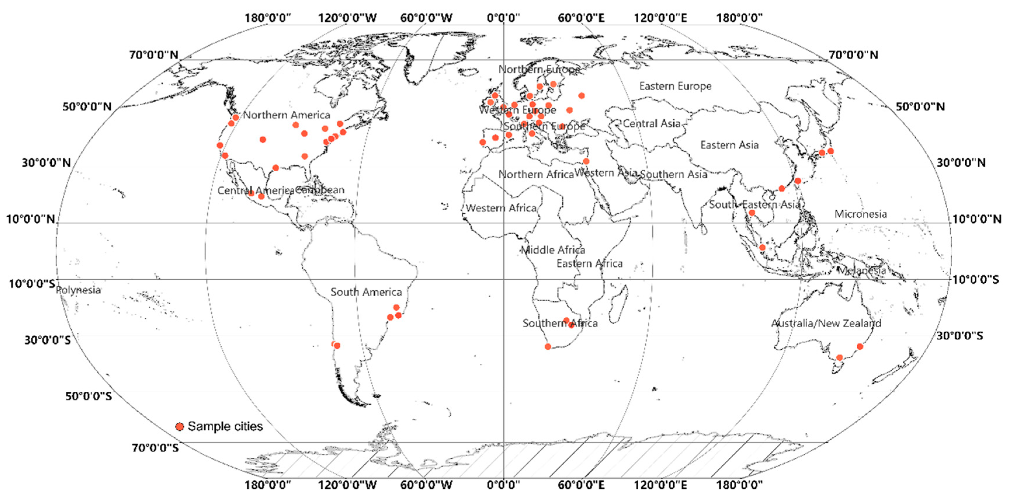
2.1. Study Area
2.2. Description of Data Sources
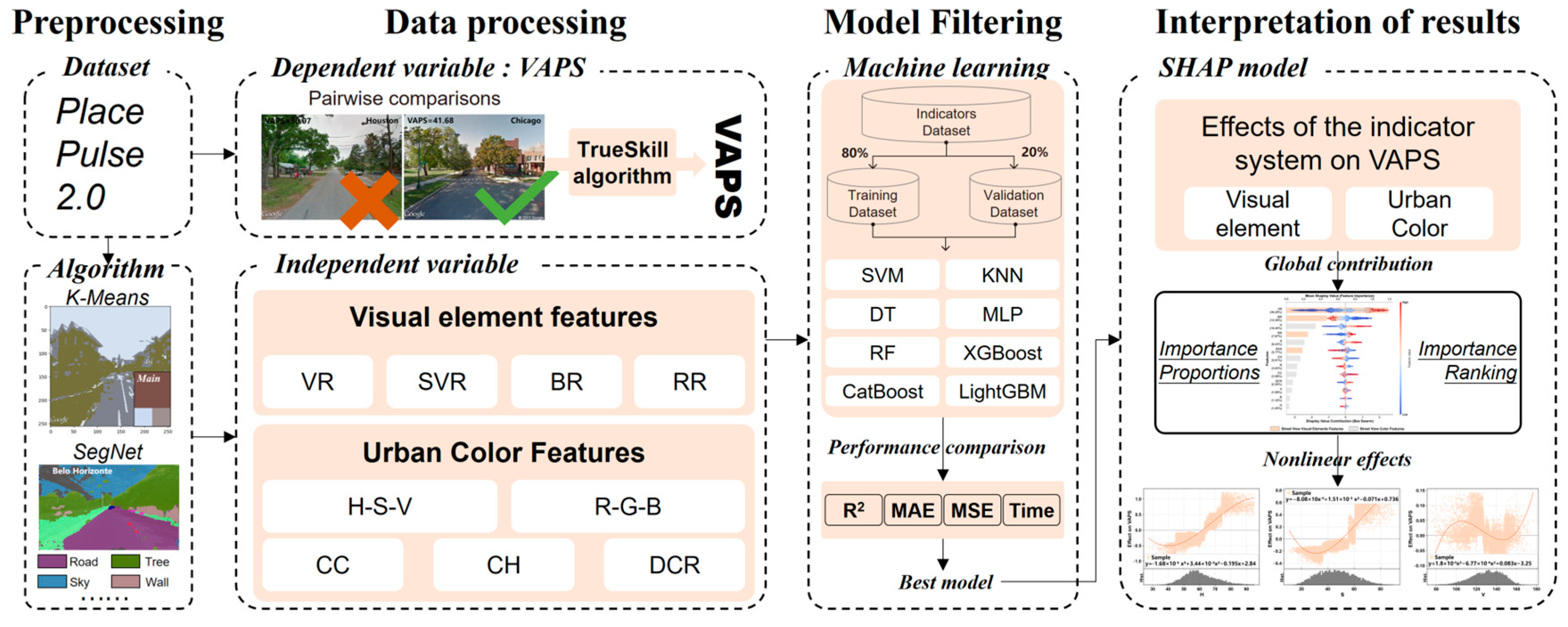
2.3. Research Methods Process
2.3.1. Urban Color Features
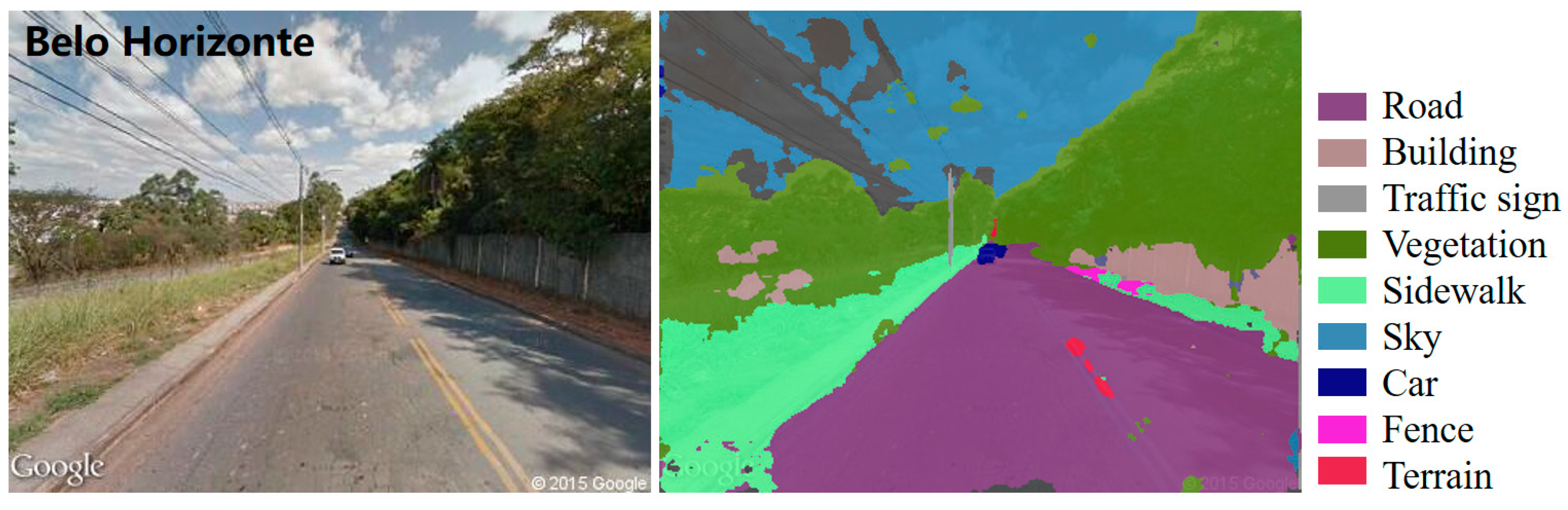
2.3.2. Urban Visual Elements Features
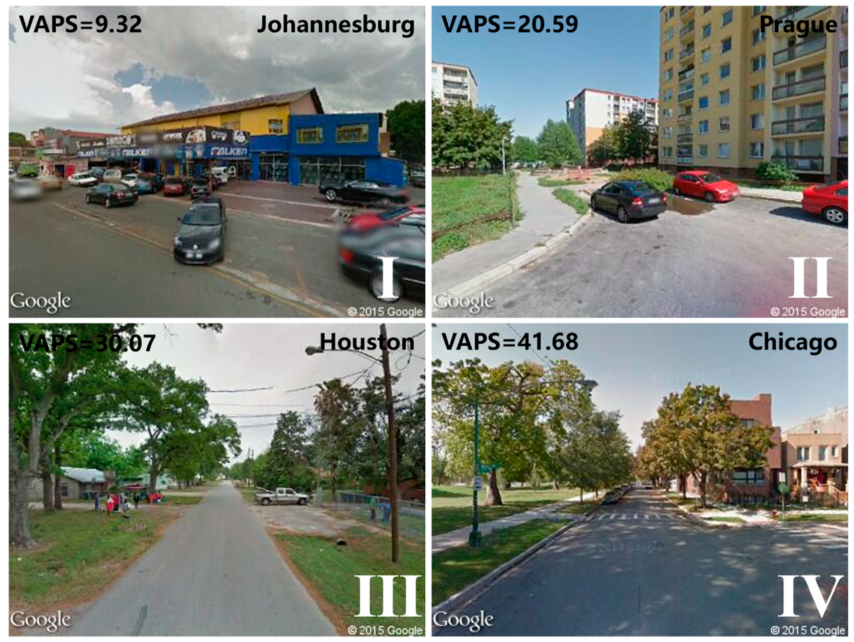
2.3.3. Visual Aesthetic Perception Score
2.3.4. VAPS Decoupling Empirical Model
2.3.5. Interpretation of Driving Factor of VAPS
3. Results
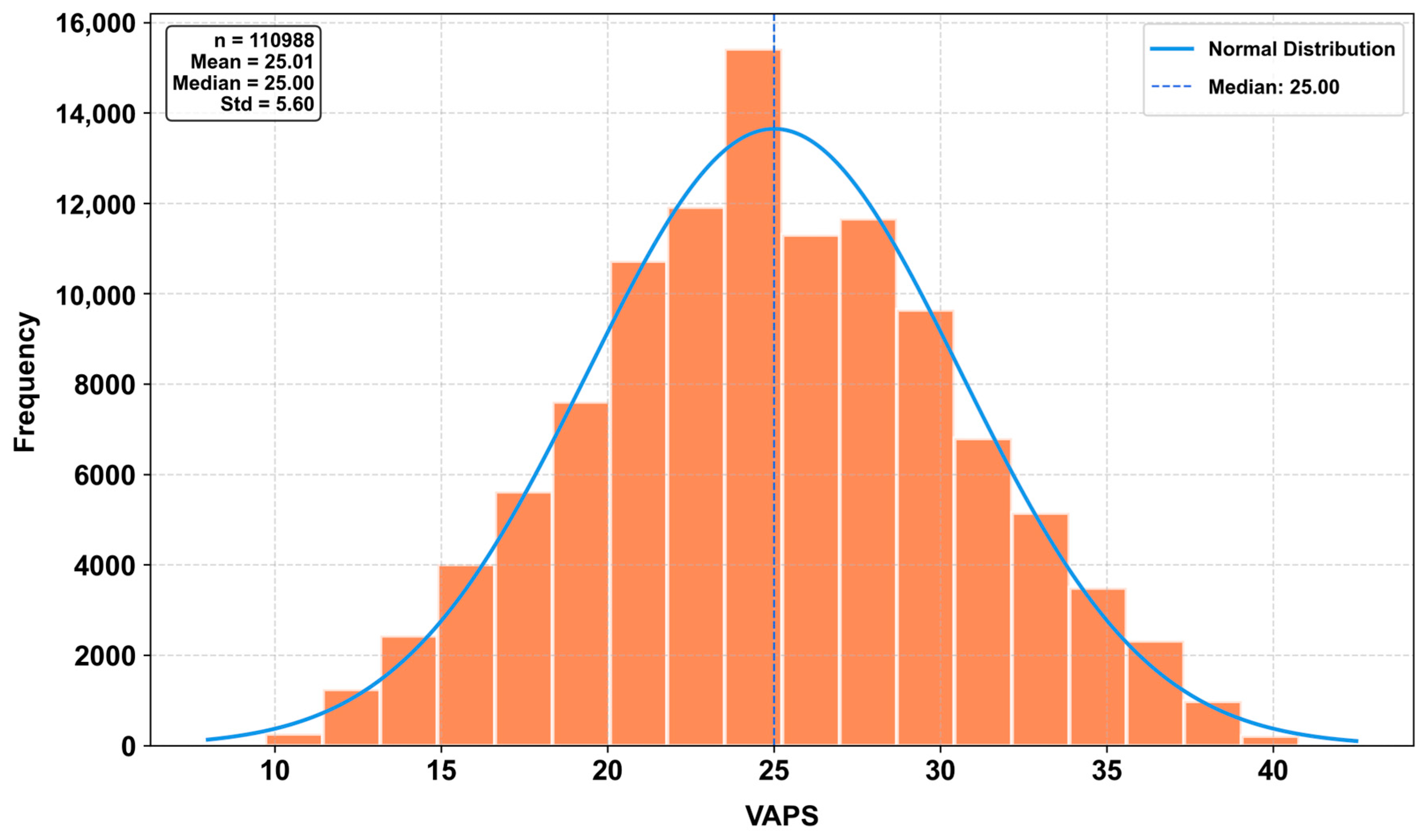
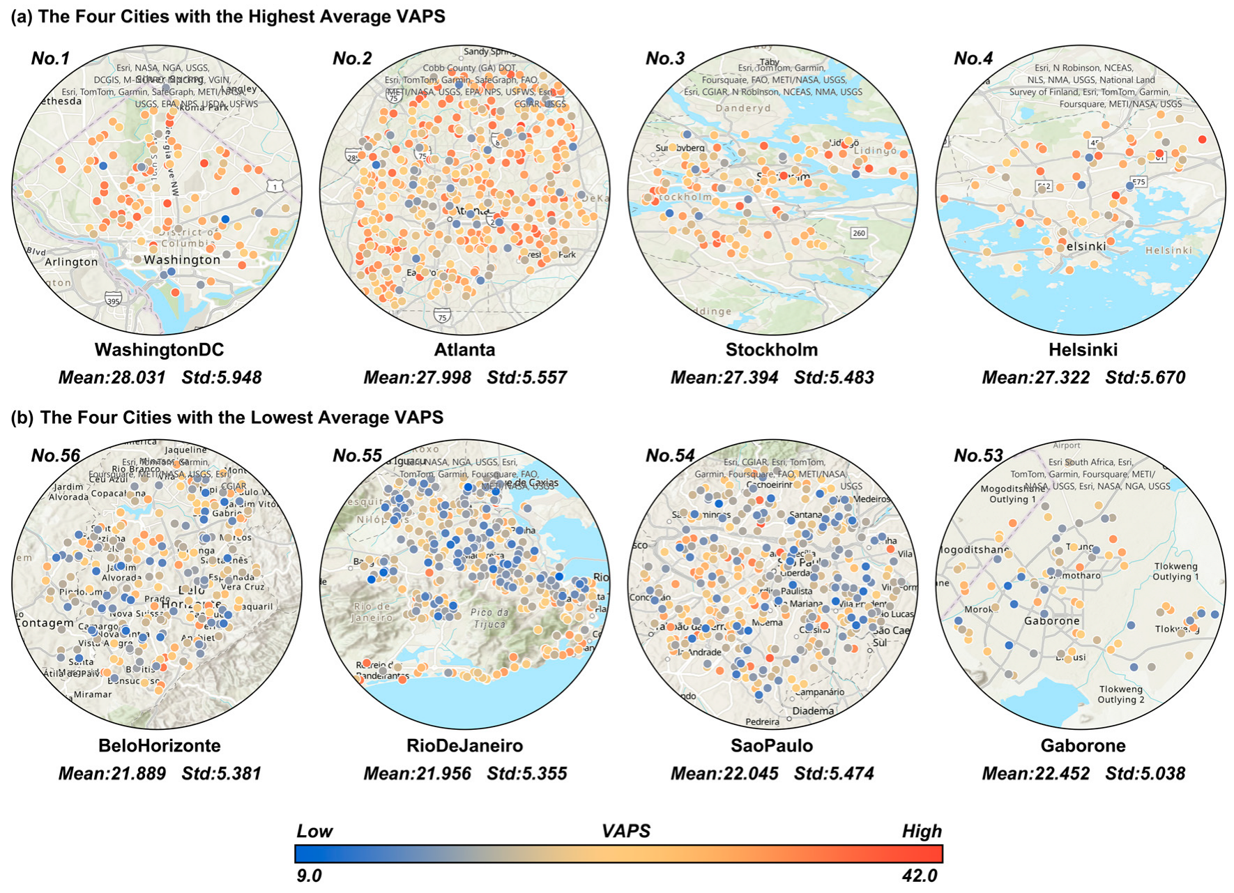
3.1. Distribution of VAPS
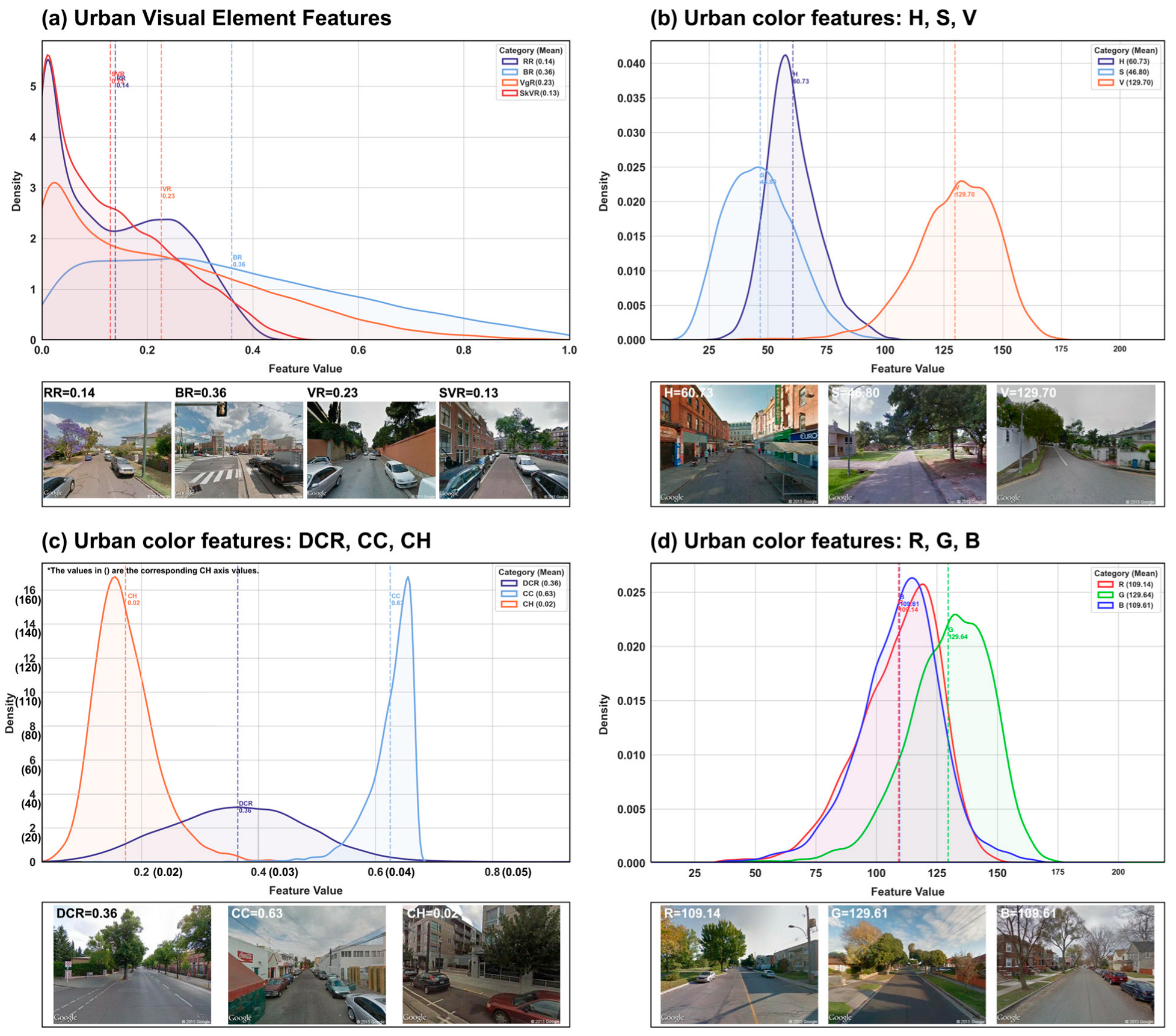
3.2. Distribution of Street-View Color and Visual Element Features
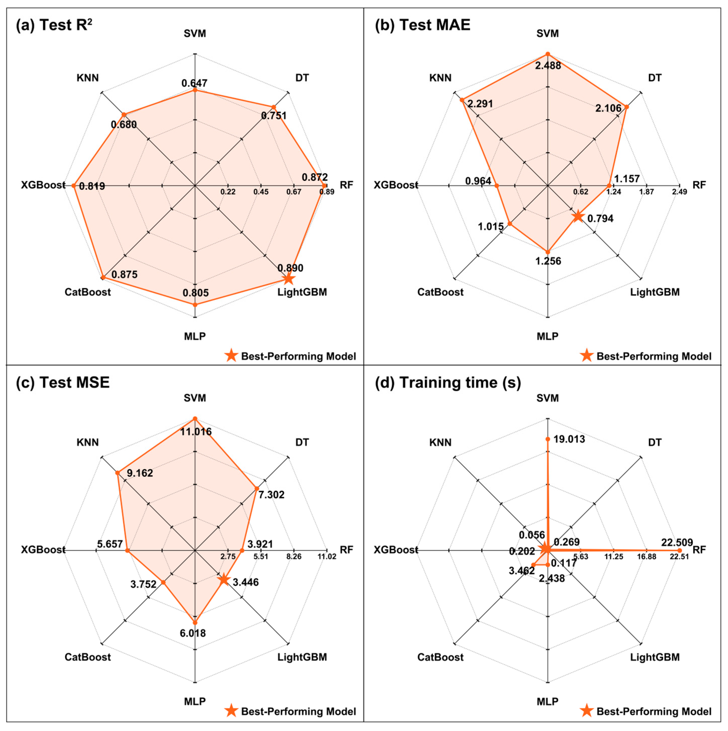
3.3. Performance Comparison of Different Machine Learning Decoupling Models
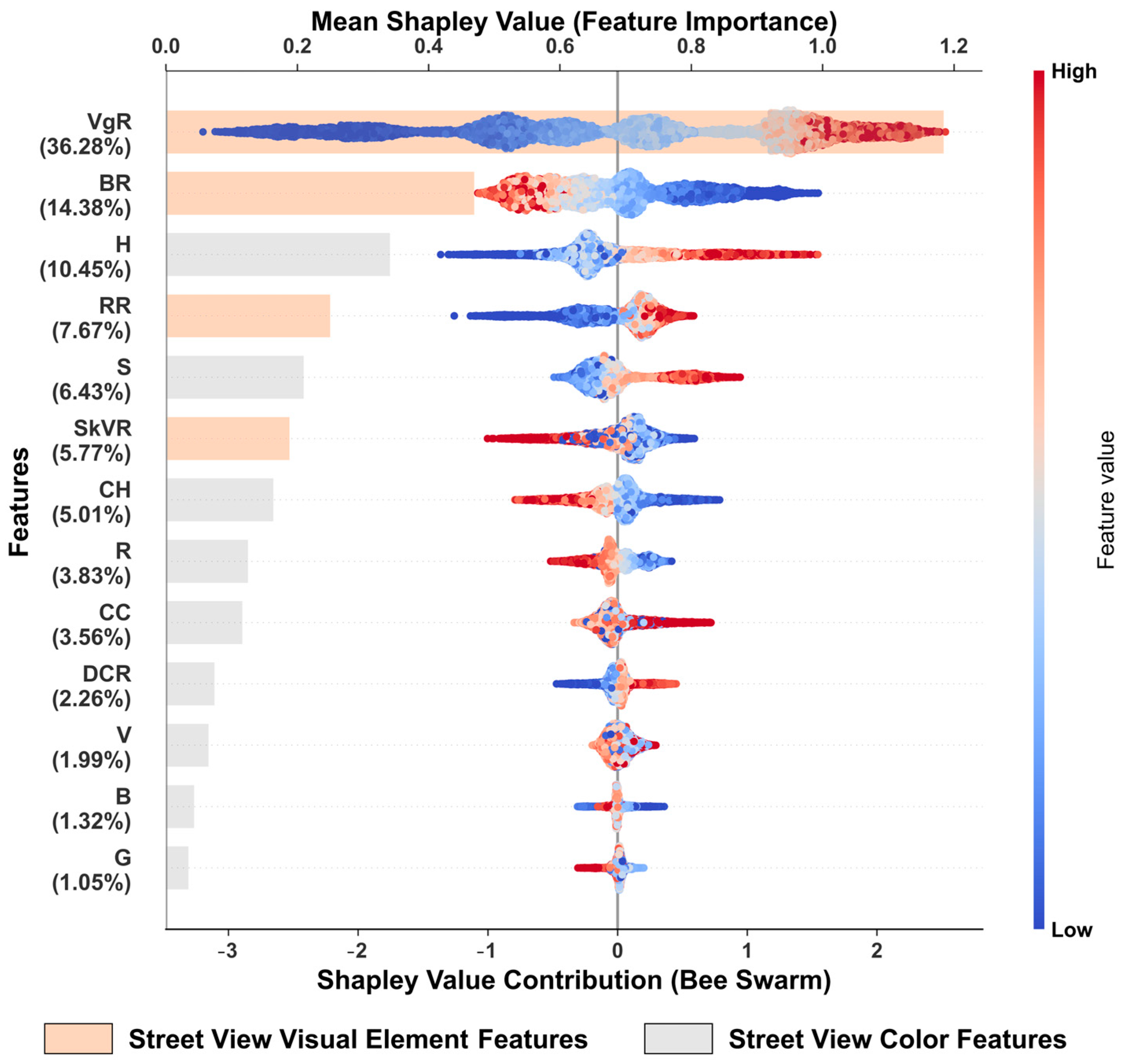
3.4. Analysis of Overall Feature Contribution
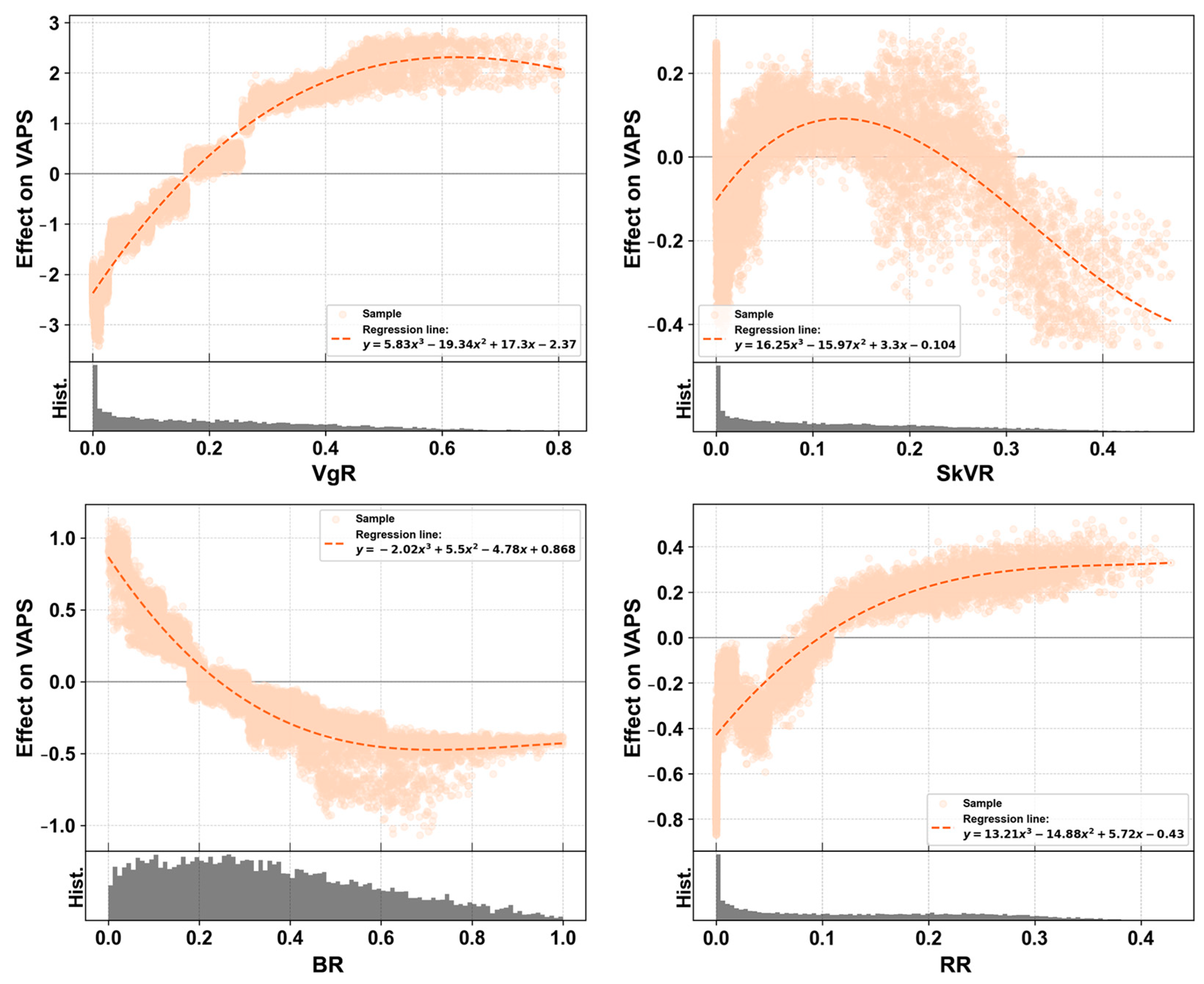
3.5. Nonlinear Effects
3.5.1. Nonlinear Effects of Street-View Visual Element Features on VAPS
3.5.2. Nonlinear Effects of Street-View Color Features on VAPS
4. Discussion
4.1. The Importance of Street Vegetation Visibility Ratio
4.2. Preferences in the Composition of Urban Street-View Visual Elements
4.3. Preferences in Urban Color for Different Populations
4.4. Limitations and Future Prospects
5. Conclusions
Supplementary Materials
Author Contributions
Funding
Data Availability Statement
Conflicts of Interest
References
- Chen, Z.; Qiao, R.; Li, S.; Zhou, S.; Zhang, X.; Wu, Z.; Wu, T. Heat and Mobility: Machine Learning Perspectives on Bike-Sharing Resilience in Shanghai. Transp. Res. Part D Transp. Environ. 2025, 142, 104692. [Google Scholar] [CrossRef]
- Li, X.; Qin, J.; Long, Y. Urban Architectural Color Evaluation: A Cognitive Framework Combining Machine Learning and Human Perception. Buildings 2024, 14, 3901. [Google Scholar] [CrossRef]
- Tosca, T.F. Environmental Colour Design for the Third Millennium: An Evolutionary Standpoint. Color Res. Appl. 2002, 27, 441–454. [Google Scholar] [CrossRef]
- Zhang, C.; Tan, G. Quantifying Architectural Color Quality: A Machine Learning Integrated Framework Driven by Quantitative Color Metrics. Ecol. Indic. 2023, 157, 111237. [Google Scholar] [CrossRef]
- McLellan, G.; Guaralda, M. Exploring Environmental Colour Design in Urban Contexts. J. Public Space 2018, 3, 93–102. [Google Scholar] [CrossRef]
- Zhang, J.; Aziz, F.A.; Hasna, M.F. Exploring the Influence of Color Preference on Urban Vitality: A Review of the Role of Color in Regulating Pedestrian Streets. Tuijin Jishu/J. Propuls. Technol. 2023, 44, 4033–4043. [Google Scholar] [CrossRef]
- Jeong, J.S.; Montero-Parejo, M.J.; García-Moruno, L.; Hernández-Blanco, J. The Visual Evaluation of Rural Areas: A Methodological Approach for the Spatial Planning and Color Design of Scattered Second Homes with an Example in Hervás, Western Spain. Land Use Policy 2015, 46, 330–340. [Google Scholar] [CrossRef]
- Mehanna, W.A.E.-H.; Mehanna, W.A.E.-H. Urban Renewal for Traditional Commercial Streets at the Historical Centers of Cities. Alex. Eng. J. 2019, 58, 1127–1143. [Google Scholar] [CrossRef]
- Bian, W. Study on the Characteristics and the Causes of Urban Color Evolution Based on New Contextualism. IOP Conf. Ser. Earth Environ. Sci. 2018, 189, 062071. [Google Scholar] [CrossRef]
- Park, K.; Ewing, R.; Sabouri, S.; Larsen, J. Street Life and the Built Environment in an Auto-Oriented US Region. Cities 2019, 88, 243–251. [Google Scholar] [CrossRef]
- Cavalcante, A.; Mansouri, A.; Kacha, L.; Barros, A.K.; Takeuchi, Y.; Matsumoto, N.; Ohnishi, N. Measuring Streetscape Complexity Based on the Statistics of Local Contrast and Spatial Frequency. PLoS ONE 2014, 9, e87097. [Google Scholar] [CrossRef] [PubMed]
- Chen, Q.; Cheng, Q.; Chen, Y.; Li, K.; Wang, D.; Cao, S. The Influence of Sky View Factor on Daytime and Nighttime Urban Land Surface Temperature in Different Spatial-Temporal Scales: A Case Study of Beijing. Remote Sens. 2021, 13, 4117. [Google Scholar] [CrossRef]
- Kaplan, R.; Kaplan, S. The Experience of Nature: A Psychological Perspective; CUP Archive: New York, NY, USA, 1989; ISBN 978-0-521-34939-0. [Google Scholar]
- Wohlwill, J.F. Environmental Aesthetics: The Environment as a Source of Affect. In Human Behavior and Environment: Advances in Theory and Research. Volume 1; Altman, I., Wohlwill, J.F., Eds.; Springer: Boston, MA, USA, 1976; pp. 37–86. ISBN 978-1-4684-2550-5. [Google Scholar]
- Ulrich, R.S. Aesthetic and Affective Response to Natural Environment. In Behavior and the Natural Environment; Altman, I., Wohlwill, J.F., Eds.; Springer: Boston, MA, USA, 1983; pp. 85–125. ISBN 978-1-4613-3539-9. [Google Scholar]
- Kacha, L.; Matsumoto, N.; Mansouri, A. Electrophysiological Evaluation of Perceived Complexity in Streetscapes. J. Asian Archit. Build. Eng. 2015, 14, 585–592. [Google Scholar] [CrossRef]
- Ma, X.; Ma, C.; Wu, C.; Xi, Y.; Yang, R.; Peng, N.; Zhang, C.; Ren, F. Measuring Human Perceptions of Streetscapes to Better Inform Urban Renewal: A Perspective of Scene Semantic Parsing. Cities 2021, 110, 103086. [Google Scholar] [CrossRef]
- Han, X.; Wang, L.; Seo, S.H.; He, J.; Jung, T. Measuring Perceived Psychological Stress in Urban Built Environments Using Google Street View and Deep Learning. Front. Public Health 2022, 10, 891736. [Google Scholar] [CrossRef]
- Dong, R.; Zhang, Y.; Zhao, J. How Green Are the Streets Within the Sixth Ring Road of Beijing? An Analysis Based on Tencent Street View Pictures and the Green View Index. Int. J. Environ. Res. Public Health 2018, 15, 1367. [Google Scholar] [CrossRef] [PubMed]
- Chen, X.; Meng, Q.; Hu, D.; Zhang, L.; Yang, J. Evaluating Greenery around Streets Using Baidu Panoramic Street View Images and the Panoramic Green View Index. Forests 2019, 10, 1109. [Google Scholar] [CrossRef]
- Beil, K.; Hanes, D. The Influence of Urban Natural and Built Environments on Physiological and Psychological Measures of Stress—A Pilot Study. Int. J. Environ. Res. Public Health 2013, 10, 1250–1267. [Google Scholar] [CrossRef] [PubMed]
- Chen, Z.; Li, S.; Liu, C. Challenges and Potentials: Environmental Assessment of Particulate Matter in Spaces Under Highway Viaducts. Atmosphere 2024, 15, 1325. [Google Scholar] [CrossRef]
- Gao, M.; Fang, C. Pedaling through the Cityscape: Unveiling the Association of Urban Environment and Cycling Volume through Street View Imagery Analysis. Cities 2025, 156, 105573. [Google Scholar] [CrossRef]
- Jiang, B.; Larsen, L.; Deal, B.; Sullivan, W.C. A Dose–Response Curve Describing the Relationship between Tree Cover Density and Landscape Preference. Landsc. Urban Plan. 2015, 139, 16–25. [Google Scholar] [CrossRef]
- Mahmoudi, M.; Ahmad, F.; Abbasi, B. Livable Streets: The Effects of Physical Problems on the Quality and Livability of Kuala Lumpur Streets. Cities 2015, 43, 104–114. [Google Scholar] [CrossRef]
- Ito, K.; Biljecki, F. Assessing Bikeability with Street View Imagery and Computer Vision. Transp. Res. Part C Emerg. Technol. 2021, 132, 103371. [Google Scholar] [CrossRef]
- Tang, J.; Long, Y. Measuring Visual Quality of Street Space and Its Temporal Variation: Methodology and Its Application in the Hutong Area in Beijing. Landsc. Urban Plan. 2019, 191, 103436. [Google Scholar] [CrossRef]
- Wang, R.; Lu, Y.; Zhang, J.; Liu, P.; Yao, Y.; Liu, Y. The Relationship between Visual Enclosure for Neighbourhood Street Walkability and Elders’ Mental Health in China: Using Street View Images. J. Transp. Health 2019, 13, 90–102. [Google Scholar] [CrossRef]
- Wan, J.; Zhou, Y.; Li, Y.; Su, Y.; Cao, Y.; Zhang, L.; Ying, L.; Deng, W. Research on Color Space Perceptions and Restorative Effects of Blue Space Based on Color Psychology: Examination of the Yijie District of Dujiangyan City as an Example. Int. J. Environ. Res. Public Health 2020, 17, 3137. [Google Scholar] [CrossRef]
- Grossman, I.; Bandara, K.; Wilson, T.; Kirley, M. Can Machine Learning Improve Small Area Population Forecasts? A Forecast Combination Approach. Comput. Environ. Urban Syst. 2022, 95, 101806. [Google Scholar] [CrossRef]
- Pang, B.; Nijkamp, E.; Wu, Y.N. Deep Learning With TensorFlow: A Review. J. Educ. Behav. Stat. 2020, 45, 227–248. [Google Scholar] [CrossRef]
- Rui, J.; Cai, C.; Wu, Y. Towards Equal Neighborhood Evolution? A Longitudinal Study of Soundscape and Visual Evolution and Housing Value Fluctuations in Shenzhen. J. Environ. Manag. 2024, 370, 122829. [Google Scholar] [CrossRef]
- Goel, R.; Garcia, L.M.T.; Goodman, A.; Johnson, R.; Aldred, R.; Murugesan, M.; Brage, S.; Bhalla, K.; Woodcock, J. Estimating City-Level Travel Patterns Using Street Imagery: A Case Study of Using Google Street View in Britain. PLoS ONE 2018, 13, e0196521. [Google Scholar] [CrossRef]
- Hu, C.-B.; Zhang, F.; Gong, F.-Y.; Ratti, C.; Li, X. Classification and Mapping of Urban Canyon Geometry Using Google Street View Images and Deep Multitask Learning. Build. Environ. 2020, 167, 106424. [Google Scholar] [CrossRef]
- Lu, Y. Using Google Street View to Investigate the Association between Street Greenery and Physical Activity. Landsc. Urban Plan. 2019, 191, 103435. [Google Scholar] [CrossRef]
- Wu, C.; Peng, N.; Ma, X.; Li, S.; Rao, J. Assessing Multiscale Visual Appearance Characteristics of Neighbourhoods Using Geographically Weighted Principal Component Analysis in Shenzhen, China. Comput. Environ. Urban Syst. 2020, 84, 101547. [Google Scholar] [CrossRef]
- Li, X.; Ratti, C.; Seiferling, I. Mapping Urban Landscapes Along Streets Using Google Street View. In Advances in Cartography and GIScience; Peterson, M.P., Ed.; Springer International Publishing: Cham, Switzerland, 2017; pp. 341–356. [Google Scholar]
- Ye, Y.; Richards, D.; Lu, Y.; Song, X.; Zhuang, Y.; Zeng, W.; Zhong, T. Measuring Daily Accessed Street Greenery: A Human-Scale Approach for Informing Better Urban Planning Practices. Landsc. Urban Plan. 2019, 191, 103434. [Google Scholar] [CrossRef]
- Wang, R.; Liu, Y.; Lu, Y.; Zhang, J.; Liu, P.; Yao, Y.; Grekousis, G. Perceptions of Built Environment and Health Outcomes for Older Chinese in Beijing: A Big Data Approach with Street View Images and Deep Learning Technique. Comput. Environ. Urban Syst. 2019, 78, 101386. [Google Scholar] [CrossRef]
- Su, S.; Zhou, H.; Xu, M.; Ru, H.; Wang, W.; Weng, M. Auditing Street Walkability and Associated Social Inequalities for Planning Implications. J. Transp. Geogr. 2019, 74, 62–76. [Google Scholar] [CrossRef]
- Faouzi, J.; Colliot, O. Classic Machine Learning Methods. In Machine Learning for Brain Disorders; Colliot, O., Ed.; Springer: New York, NY, USA, 2023; pp. 25–75. ISBN 978-1-0716-3195-9. [Google Scholar]
- Ke, G.; Meng, Q.; Finley, T.; Wang, T.; Chen, W.; Ma, W.; Ye, Q.; Liu, T.-Y. LightGBM: A Highly Efficient Gradient Boosting Decision Tree. In Advances in Neural Information Processing Systems; Curran Associates, Inc.: New York, NY, USA, 2017; Volume 30. [Google Scholar]
- Rigatti, S.J. Random Forest. J. Insur. Med. 2017, 47, 31–39. [Google Scholar] [CrossRef]
- Chen, T.; Guestrin, C. XGBoost: A Scalable Tree Boosting System. In Proceedings of the 22nd ACM SIGKDD International Conference on Knowledge Discovery and Data Mining, San Francisco, CA, USA, 13–17 August 2016; Association for Computing Machinery: New York, NY, USA, 13 August 2016; pp. 785–794. [Google Scholar]
- Hancock, J.T.; Khoshgoftaar, T.M. CatBoost for Big Data: An Interdisciplinary Review. J Big Data 2020, 7, 94. [Google Scholar] [CrossRef]
- Noble, W.S. What Is a Support Vector Machine? Nat. Biotechnol. 2006, 24, 1565–1567. [Google Scholar] [CrossRef]
- Kramer, O. (Ed.) K-Nearest Neighbors. In Dimensionality Reduction with Unsupervised Nearest Neighbors; Springer: Berlin/Heidelberg, Germany, 2013; pp. 13–23. ISBN 978-3-642-38652-7. [Google Scholar]
- Taud, H.; Mas, J.F. Multilayer Perceptron (MLP). In Geomatic Approaches for Modeling Land Change Scenarios; Camacho Olmedo, M.T., Paegelow, M., Mas, J.-F., Escobar, F., Eds.; Springer International Publishing: Cham, Switzerland, 2018; pp. 451–455. ISBN 978-3-319-60801-3. [Google Scholar]
- Charbuty, B.; Abdulazeez, A. Classification Based on Decision Tree Algorithm for Machine Learning. J. Appl. Sci. Technol. Trends 2021, 2, 20–28. [Google Scholar] [CrossRef]
- Zhang, S.; Liu, N.; Ma, B.; Yan, S. The Effects of Street Environment Features on Road Running: An Analysis Using Crowdsourced Fitness Tracker Data and Machine Learning. Environ. Plan. B 2024, 51, 529–545. [Google Scholar] [CrossRef]
- Gao, M.; Fang, C. Deciphering Urban Cycling: Analyzing the Nonlinear Impact of Street Environments on Cycling Volume Using Crowdsourced Tracker Data and Machine Learning. J. Transp. Geogr. 2025, 124, 104179. [Google Scholar] [CrossRef]
- Nguyen, L.; Teller, J. Color in the Urban Environment: A User-Oriented Protocol for Chromatic Characterization and the Development of a Parametric Typology. Color Res. Appl. 2017, 42, 131–142. [Google Scholar] [CrossRef]
- Chen, L.; Kong, F. Quantitative Method of Regional Color Planning—Field Investigation on Renewal Design of Jiangchuan Street. In Advances in Creativity, Innovation, Entrepreneurship and Communication of Design; Markopoulos, E., Goonetilleke, R.S., Ho, A.G., Luximon, Y., Eds.; Springer International Publishing: Cham, Switzerland, 2021; pp. 608–617. [Google Scholar]
- Wang, J.; Zhang, L.; Gou, A. Study of the Color Characteristics of Residential Buildings in Shanghai. Color Res. Appl. 2021, 46, 240–257. [Google Scholar] [CrossRef]
- Zhong, T.; Ye, C.; Wang, Z.; Tang, G.; Zhang, W.; Ye, Y. City-Scale Mapping of Urban Façade Color Using Street-View Imagery. Remote Sens. 2021, 13, 1591. [Google Scholar] [CrossRef]
- McGinn, A.P.; Evenson, K.R.; Herring, A.H.; Huston, S.L.; Rodriguez, D.A. Exploring Associations between Physical Activity and Perceived and Objective Measures of the Built Environment. J. Urban Health 2007, 84, 162–184. [Google Scholar] [CrossRef] [PubMed]
- Zhou, H.; He, S.; Cai, Y.; Wang, M.; Su, S. Social Inequalities in Neighborhood Visual Walkability: Using Street View Imagery and Deep Learning Technologies to Facilitate Healthy City Planning. Sustain. Cities Soc. 2019, 50, 101605. [Google Scholar] [CrossRef]
- Dubey, A.; Naik, N.; Parikh, D.; Raskar, R.; Hidalgo, C.A. Deep Learning the City: Quantifying Urban Perception At A Global Scale. In Proceedings of the Computer Vision–ECCV 2016: 14th European Conference, Amsterdam, The Netherlands, 11–14 October 2016. [Google Scholar]
- Salesses, P.; Schechtner, K.; Hidalgo, C.A. The Collaborative Image of The City: Mapping the Inequality of Urban Perception. PLoS ONE 2013, 8, e68400. [Google Scholar] [CrossRef]
- Kiapour, M.H.; Yamaguchi, K.; Berg, A.C.; Berg, T.L. Hipster Wars: Discovering Elements of Fashion Styles. In Computer Vision—ECCV 2014; Fleet, D., Pajdla, T., Schiele, B., Tuytelaars, T., Eds.; Lecture Notes in Computer Science; Springer International Publishing: Cham, Switzerland, 2014; Volume 8689, pp. 472–488. ISBN 978-3-319-10589-5. [Google Scholar]
- Naik, N.; Philipoom, J.; Raskar, R.; Hidalgo, C. Streetscore—Predicting the Perceived Safety of One Million Streetscapes. In Proceedings of the 2014 IEEE Conference on Computer Vision and Pattern Recognition Workshops, Columbus, OH, USA, 23–28 June 2014; pp. 793–799. [Google Scholar]
- Jou, B.; Bhattacharya, S.; Chang, S.-F. Predicting Viewer Perceived Emotions in Animated GIFs. In Proceedings of the 22nd ACM International Conference on Multimedia, Orlando, FL, USA, 3 November 2014; ACM: Orlando, FL, USA, 2014; pp. 213–216. [Google Scholar]
- Sartori, A.; Yanulevskaya, V.; Salah, A.A.; Uijlings, J.; Bruni, E.; Sebe, N. Affective Analysis of Professional and Amateur Abstract Paintings Using Statistical Analysis and Art Theory. ACM Trans. Interact. Intell. Syst. (TiiS) 2015, 5, 1–27. [Google Scholar] [CrossRef]
- Bijmolt, T.H.; Wedel, M. The Effects of Alternative Methods of Collecting Similarity Data for Multidimensional Scaling. Int. J. Res. Mark. 1995, 12, 363–371. [Google Scholar] [CrossRef]
- Stewart, N.; Brown, G.D.; Chater, N. Absolute Identification by Relative Judgment. Psychol. Rev. 2005, 112, 881. [Google Scholar] [CrossRef] [PubMed]
- Gunduz, A.B.; Taskin, B.; Yavuz, A.G.; Karsligil, M.E. A Better Way of Extracting Dominant Colors Using Salient Objects with Semantic Segmentation. Eng. Appl. Artif. Intell. 2021, 100, 104204. [Google Scholar] [CrossRef]
- Qi, Z.; Li, J.; He, Z. The Influence of Urban Streetscape Color on Tourists’ Emotional Perception Based on Streetscape Images. J. Geo Inf. Sci. 2024, 26, 514–529. [Google Scholar]
- Wei, S.-T.; Ou, L.-C.; Luo, M.R.; Hutchings, J.B. Package Design: Colour Harmony and Consumer Expectations. Int. J. Des. 2014, 8, 109–126. [Google Scholar]
- Badrinarayanan, V.; Kendall, A.; Cipolla, R. Segnet: A Deep Convolutional Encoder-Decoder Architecture for Image Segmentation. IEEE Trans. Pattern Anal. Mach. Intell. 2017, 39, 2481–2495. [Google Scholar] [CrossRef]
- Yin, L.; Wang, Z. Measuring Visual Enclosure for Street Walkability: Using Machine Learning Algorithms and Google Street View Imagery. Appl. Geogr. 2016, 76, 147–153. [Google Scholar] [CrossRef]
- Li, X.; Zhang, C.; Li, W.; Ricard, R.; Meng, Q.; Zhang, W. Assessing Street-Level Urban Greenery Using Google Street View and a Modified Green View Index. Urban For. Urban Green. 2015, 14, 675–685. [Google Scholar] [CrossRef]
- Herbrich, R.; Minka, T.; Graepel, T. TrueSkillTM: A Bayesian Skill Rating System. In Advances in Neural Information Processing Systems 19, Proceedings of the 2006 Conference, Vancouver, BC, Canada, 4–7 December 2006; MIT Press: Cambridge, MA, USA, 2006; Volume 19. [Google Scholar] [CrossRef]
- Shekhar, S.; Bansode, A.; Salim, A. A Comparative Study of Hyper-Parameter Optimization Tools. In Proceedings of the 2021 IEEE Asia-Pacific Conference on Computer Science and Data Engineering (CSDE), Brisbane, Australia, 8–10 December 2021; pp. 1–6. [Google Scholar]
- Rastogi, D.; Johri, P.; Tiwari, V.; Elngar, A.A. Multi-Class Classification of Brain Tumour Magnetic Resonance Images Using Multi-Branch Network with Inception Block and Five-Fold Cross Validation Deep Learning Framework. Biomed. Signal Process. Control 2024, 88, 105602. [Google Scholar] [CrossRef]
- Aggarwal, A.; Lohia, P.; Nagar, S.; Dey, K.; Saha, D. Black Box Fairness Testing of Machine Learning Models. In Proceedings of the 2019 27th ACM Joint Meeting on European Software Engineering Conference and Symposium on the Foundations of Software Engineering, Tallinn, Estonia, 26–30 August 2019; Association for Computing Machinery: New York, NY, USA, 2019; pp. 625–635. [Google Scholar]
- Lundberg, S.M.; Erion, G.; Chen, H.; DeGrave, A.; Prutkin, J.M.; Nair, B.; Katz, R.; Himmelfarb, J.; Bansal, N.; Lee, S.-I. From Local Explanations to Global Understanding with Explainable AI for Trees. Nat. Mach. Intell. 2020, 2, 56–67. [Google Scholar] [CrossRef]
- Rajagopal, P.; Priya, R.S.; Senthil, R. A Review of Recent Developments in the Impact of Environmental Measures on Urban Heat Island. Sustain. Cities Soc. 2023, 88, 104279. [Google Scholar] [CrossRef]
- Biljecki, F.; Ito, K. Street View Imagery in Urban Analytics and GIS: A Review. Landsc. Urban Plan. 2021, 215, 104217. [Google Scholar] [CrossRef]
- Helbich, M.; Poppe, R.; Oberski, D.; Zeylmans Van Emmichoven, M.; Schram, R. Can’t See the Wood for the Trees? An Assessment of Street View- and Satellite-Derived Greenness Measures in Relation to Mental Health. Landsc. Urban Plan. 2021, 214, 104181. [Google Scholar] [CrossRef]
- Xie, X.; Jiang, Q.; Wang, R.; Gou, Z. Correlation between Vegetation Landscape and Subjective Human Perception: A Systematic Review. Buildings 2024, 14, 1734. [Google Scholar] [CrossRef]
- Zhang, L.; Tan, P.Y.; Richards, D. Relative Importance of Quantitative and Qualitative Aspects of Urban Green Spaces in Promoting Health. Landsc. Urban Plan. 2021, 213, 104131. [Google Scholar] [CrossRef]
- Lin, W.; Zeng, C.; Bao, Z.; Jin, H. The Therapeutic Look up: Stress Reduction and Attention Restoration Vary According to the Sky-Leaf-Trunk (SLT) Ratio in Canopy Landscapes. Landsc. Urban Plan. 2023, 234, 104730. [Google Scholar] [CrossRef]
- Zhao, M.; Zhang, Y. Exploring the Dose-Response of Landscape Preference: A Case Study in Singapore. Appl. Geogr. 2024, 170, 103357. [Google Scholar] [CrossRef]
- Jorgensen, A.; Hitchmough, J.; Calvert, T. Woodland Spaces and Edges: Their Impact on Perception of Safety and Preference. Landsc. Urban Plan. 2002, 60, 135–150. [Google Scholar] [CrossRef]
- Lis, A.; Pardela, Ł.; Iwankowski, P. Impact of Vegetation on Perceived Safety and Preference in City Parks. Sustainability 2019, 11, 6324. [Google Scholar] [CrossRef]
- Ogawa, Y.; Oki, T.; Zhao, C.; Sekimoto, Y.; Shimizu, C. Evaluating the Subjective Perceptions of Streetscapes Using Street-View Images. Landsc. Urban Plan. 2024, 247, 105073. [Google Scholar] [CrossRef]
- Tang, F.; Zeng, P.; Wang, L.; Zhang, L.; Xu, W. Urban Perception Evaluation and Street Refinement Governance Supported by Street View Visual Elements Analysis. Remote Sens. 2024, 16, 3661. [Google Scholar] [CrossRef]
- Liu, C.; Yu, Y.; Yang, X. Perceptual Evaluation of Street Quality in Underdeveloped Ethnic Areas: A Random Forest Method Combined with Human–Machine Confrontation Framework Provides Insights for Improved Urban Planning—A Case Study of Lhasa City. Buildings 2024, 14, 1698. [Google Scholar] [CrossRef]
- Zhang, J.; Heng, C.K.; Malone-Lee, L.C.; Hii, D.J.C.; Janssen, P.; Leung, K.S.; Tan, B.K. Evaluating Environmental Implications of Density: A Comparative Case Study on the Relationship between Density, Urban Block Typology and Sky Exposure. Autom. Constr. 2012, 22, 90–101. [Google Scholar] [CrossRef]
- Fitzpatrick, M. Bridging Theories, William H. Whyte and the Sorcery of Cities. Archit. Cult. 2016, 4, 381–393. [Google Scholar] [CrossRef]
- Valdez, P.; Mehrabian, A. Effects of Color on Emotions. J. Exp. Psychol. Gen. 1994, 123, 394–409. [Google Scholar] [CrossRef] [PubMed]
- Yu, M.; Zheng, X.; Qin, P.; Cui, W.; Ji, Q. Urban Color Perception and Sentiment Analysis Based on Deep Learning and Street View Big Data. Appl. Sci. 2024, 14, 9521. [Google Scholar] [CrossRef]
- Zhang, S.; Liu, Y.; Nie, H. Geographical Feature Based Research on Urban Color Environment—Taking Wuhan as an Example. IERI Procedia 2014, 9, 190–195. [Google Scholar] [CrossRef]
- Naige, C.; Xiaofan, X.; Minghong, T.; Xianming, W. A Spatial Analysis of Urban Color Harmony in Five Global Metropolises. J. Resour. Ecol. 2022, 13, 238–246. [Google Scholar] [CrossRef]
- Bellizzi, J.A.; Crowley, A.E.; Hasty, R.W. The Effects of Color in Store Design. J. Retail. 1983, 59, 21–45. [Google Scholar]
- Qi, Z.; Li, J.; Yang, X.; He, Z. How the Characteristics of Street Color Affect Visitor Emotional Experience. Comput. Urban Sci. 2025, 5, 7. [Google Scholar] [CrossRef]


| Variable Name | Description | Mean | Standard Deviation |
|---|---|---|---|
| Hue (H) | Hue value of the main clustered color in HSV color space. | 60.730 | 11.412 |
| Saturation (S) | Saturation value of the main clustered color in HSV color space. | 46.798 | 14.729 |
| Value (V) | Value (brightness) of the main clustered color in HSV color space. | 129.705 | 17.971 |
| Color Complexity Index (CC) | Index measuring the color complexity of the image (range 0–1). | 0.625 | 0.041 |
| Color Harmony Index (CH) | Index assessing the harmony of the color composition in the image. | 0.018 | 0.003 |
| Dominant Color Ratio (DCR) | Proportion of the dominant (main) clustered color in the street view. | 0.365 | 0.117 |
| Red Value (R) | Red value of the main clustered color in RGB color space. | 109.143 | 17.397 |
| Green Value (G) | Green value of the main clustered color in RGB color space. | 129.644 | 17.951 |
| Blue Value (B) | Blue value of the main clustered color in RGB color space. | 109.612 | 17.461 |
| Variable Name | Description | Mean | Standard Deviation |
| Vegetation Ratio (VgR) | Ratio of visible vegetation area to total viewable area. | 0.226 | 0.195 |
| Sky Visibility Ratio (SkVR) | Ratio of visible sky area to total viewable area. | 0.130 | 0.114 |
| Building Ratio (BR) | Ratio of visible building area to total viewable area. | 0.360 | 0.237 |
| Road Ratio (RR) | Ratio of visible road area to total viewable area. | 0.132 | 0.109 |
| Model | Training Dataset | Test Dataset | ||||
|---|---|---|---|---|---|---|
| R2 | MAE | MSE | R2 | MAE | MSE | |
| Single Urban Color Features | 0.872 | 1.897 | 3.992 | 0.852 | 1.512 | 2.592 |
| Single Urban Visual Element Features | 0.782 | 2.507 | 4.709 | 0.759 | 2.111 | 3.312 |
| Integrated Dimension | 0.958 | 0.911 | 1.310 | 0.895 | 0.964 | 3.446 |
Disclaimer/Publisher’s Note: The statements, opinions and data contained in all publications are solely those of the individual author(s) and contributor(s) and not of MDPI and/or the editor(s). MDPI and/or the editor(s) disclaim responsibility for any injury to people or property resulting from any ideas, methods, instructions or products referred to in the content. |
© 2025 by the authors. Licensee MDPI, Basel, Switzerland. This article is an open access article distributed under the terms and conditions of the Creative Commons Attribution (CC BY) license (https://creativecommons.org/licenses/by/4.0/).
Share and Cite
Wu, T.; Chen, Z.; Li, S.; Xing, P.; Wei, R.; Meng, X.; Zhao, J.; Wu, Z.; Qiao, R. Decoupling Urban Street Attractiveness: An Ensemble Learning Analysis of Color and Visual Element Contributions. Land 2025, 14, 979. https://doi.org/10.3390/land14050979
Wu T, Chen Z, Li S, Xing P, Wei R, Meng X, Zhao J, Wu Z, Qiao R. Decoupling Urban Street Attractiveness: An Ensemble Learning Analysis of Color and Visual Element Contributions. Land. 2025; 14(5):979. https://doi.org/10.3390/land14050979
Chicago/Turabian StyleWu, Tao, Zeyin Chen, Siying Li, Peixue Xing, Ruhang Wei, Xi Meng, Jingkai Zhao, Zhiqiang Wu, and Renlu Qiao. 2025. "Decoupling Urban Street Attractiveness: An Ensemble Learning Analysis of Color and Visual Element Contributions" Land 14, no. 5: 979. https://doi.org/10.3390/land14050979
APA StyleWu, T., Chen, Z., Li, S., Xing, P., Wei, R., Meng, X., Zhao, J., Wu, Z., & Qiao, R. (2025). Decoupling Urban Street Attractiveness: An Ensemble Learning Analysis of Color and Visual Element Contributions. Land, 14(5), 979. https://doi.org/10.3390/land14050979