Multi-Scale Time Series InSAR Integrated with ICA for Deciphering the Coupling Mechanism Between Groundwater Dynamics and Surface Deformation

Abstract

Land subsidence has become an increasingly serious environmental problem worldwide, especially in areas where groundwater is over-exploited. Hengshui City, as part of the North China Plain in eastern China, has been experiencing increasingly severe land subsidence due to long-term groundwater over-exploitation, which has seriously affected local infrastructure and the sustainable utilization of water resources. In order to explore the relationship between hydraulic head changes and subsidence, this study systematically analyzed the ground subsidence characteristics and its driving mechanism in the Hengshui area from January 2018 to July 2022 using the time series InSAR (interferometric synthetic aperture radar) technique combined with independent component analysis (ICA). The subsidence signals were decomposed into seasonal, trend, and stochastic features by independent component analysis, revealing the multi-scale time lag effect of hydraulic head fluctuations on subsidence. The results show that the magnitude of land subsidence is increasing under the condition of a continuously decreasing water level, reflecting the groundwater compaction problem triggered by the over-exploitation of groundwater. This study provides a theoretical basis and technical support for groundwater management and subsidence prevention and control in Hengshui and similar regions.

1. Introduction

Land subsidence is an environmental and geological phenomenon caused by the natural or anthropogenic factors of solidification and compression of underground soil, resulting in a decrease in the surface elevation of the Earth’s crust [1,2]. The fundamental cause lies in the excessive extraction of groundwater, which disrupts the hydraulic equilibrium of the aquifer system, resulting in a decrease in pore water pressure and an increase in effective stress. This process leads to the compression of aquitard and aquifer skeletal structures, ultimately triggering land subsidence [3,4,5]. With the rapid development of urban development and rapid population growth, the problem of land subsidence has emerged as an increasingly critical global environmental issue, especially in agricultural and urban areas. Since the 1920s, several regions in China have experienced different degrees of subsidence disasters, especially in the Yangtze River Delta, the North China Plain, and the Fenwei Basin, where the subsidence phenomenon continues to expand [6,7]. Hengshui City, Hebei Province, as part of the North China Plain, has an increasingly serious land subsidence problem due to the over-exploitation of groundwater resources, which has resulted in the formation of subsidence funnels, and this phenomenon continues to expand. Despite the measures taken to limit groundwater exploitation, the increase in groundwater demand has kept land subsidence from occurring at a certain rate. The rate of land subsidence in the Hengshui area is relatively fast and has a wide range of impact, with the hydraulic head of the confined aquifer declining by approximately 82.75 m, from 1.9 m below ground level in 1958 to 84.65 m below ground level in 2021, posing varying degrees of threat to water supply facilities, foundations, and transport infrastructure [8,9,10]. Against this background, how to effectively monitor and manage the land subsidence in the Hengshui area and deeply understand the interrelationship between the subsidence process and groundwater has become an urgent scientific problem.

As one of the key factors affecting surface deformation, the study of the coupling relationship between hydraulic head changes and surface deformation is of great significance for understanding the mechanism of surface deformation and predicting geological disasters. In recent years, time series InSAR technology has become an important means of surface deformation monitoring by virtue of its advantages including high precision, a large range, and continuous monitoring [11,12]. However, the time series InSAR signals often contain deformation information from multiple sources and at various spatial and temporal scales. Effectively isolating and extracting the components related to hydraulic head changes has become a difficult point in current research. Although the traditional triangular elevation measurement [13] and geodetic precision leveling method provide high-precision results, it is difficult to accurately grasp the overall distribution characteristics of subsidence due to the shortcomings of the small number of monitoring points and uneven spatial distribution, which limits its ability to detect the spatial and temporal distribution characteristics of land subsidence at the regional scale [14]. Compared with this, time series InSAR, with its all-weather monitoring, very high spatial resolution, and wide coverage, can effectively reduce the errors caused by atmospheric delay, DEM, low coherence, and other factors in the interferometric phase. Its reliability and flexibility are especially favored in land subsidence monitoring and achieve wide application [15,16].

Independent component analysis (ICA), as a blind source separation method, is able to extract statistically independent source signals from mixed signals, which provides a new idea for the extraction of multi-scale deformation information in time series InSAR [17,18]. The interferometric phase of InSAR consists of various components such as the deformation phase, terrain phase, atmospheric phase, and noise phase, so the problem of extracting signals from the interferometric phase can be regarded as the process of separating the blind source signals [19]. ICA is used to identify deformation signals induced by natural or human-induced processes and reveal the motion mechanisms under different deformation features, and it can be applied to differentiate between seasonal deformation features, trending deformation features, and other complex deformation factors. These independent signals are expected to reflect the diversity of surface deformation patterns and provide insights into their underlying driving mechanisms [20,21]. In this context, the application of independent component analysis (ICA) in the field of InSAR began in 2002, when Inglada et al. introduced ICA into InSAR research for the first time and verified the feasibility of ICA in InSAR data processing by simulating the differential interferometric phases of three consecutively disentangled interferograms and separating the atmospheric and deformation phases from the interferograms using ICA [22]. In 2006, Ballatore et al. demonstrated the advantages of ICA in extracting atmospheric artefacts and terrain residuals from deformation signals using ICA in three successively deconvolved interferometric phases [23]. In 2018, Gaddes et al. introduced blind source separation (BSS) techniques into InSAR analysis and demonstrated their potential for the automated detection and monitoring of volcanic deformation signals. Through comparative analysis with principal component analysis (PCA) and non-negative matrix factorization (NMF), their study concluded that independent component analysis (ICA) was the most effective method for decomposing InSAR time series and extracting meaningful geophysical signals [24]. In 2019, Liang et al. successfully extracted topographic residuals from deconvoluted multi-temporal interferograms using ICA. Their experiments showed that independent component analysis can estimate digital elevation model (DEM) errors without deformation a priori information and still provides reliable estimates when the observed phases are affected by atmospheric delays or the number of interferograms is limited [25].

Based on this work, this study utilized time series InSAR data with the ICA technique to derive the spatial and temporal evolution of multidimensional deformation in the Hengshui area with high accuracy. Different deformation characteristics and their mechanisms were also revealed after using ICA signal separation. The aquifer parameters and groundwater storage changes of the Hengshui region’s confined aquifer system were quantified using the InSAR technique and confined aquifer level monitoring data. An in-depth analysis of the land subsidence phenomenon in Hengshui City, identification of its main spatial and temporal deformation characteristics and driving mechanisms, combined with the hydrological characteristics of the aquifer system, comprehensively revealed the mechanism of groundwater exploitation and utilization on regional land subsidence, providing a basis for the scientific management of groundwater resources in Hengshui area, and providing theoretical support for the effective prevention, control, and technical safeguarding of land subsidence.

2. Study Area and Data

2.1. Overview of the Study Area

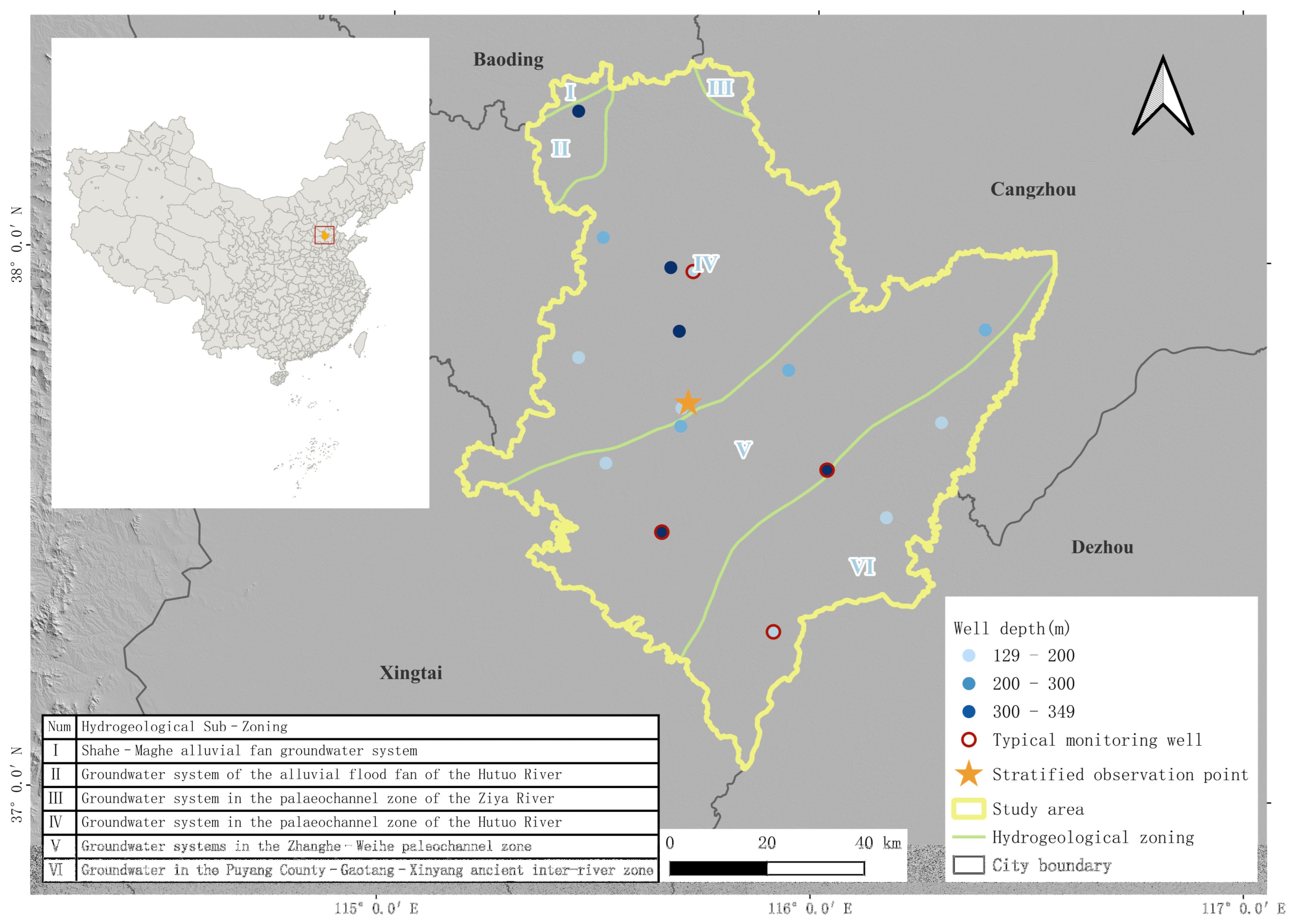
Figure 1 shows the location and hydrogeological zoning of Hengshui City, from which it is seen that Hengshui City is located in the south-central part of Hebei Province, China, at the junction of the Hebei and Shandong provinces, and neighboring Baoding City and Cangzhou City in the north and bordering Cangzhou City and Dezhou City in the east (Figure 1). The geographical coordinates are 115°11′02.08″~116°33′37.42″ E, 37°03′37.34″~38°22′11.98″ N, with a total area of about 8815 square kilometers, of which the urban area is about 30 square kilometers and 120 km away from the capital city of Shijiazhuang, which has an advantageous geographical location.

The city has a continental semi-arid monsoon climate with four distinct seasons and marked differences in temperature and humidity [26]. Summers are humid and sultry with concentrated precipitation; winters are dry and cold with sparse precipitation. The average annual temperature is about 14 °C, the annual precipitation is 550–650 mm, and the annual sunshine hours are 2430–2682 h. This climatic condition is favorable to agricultural production, but it also brings the problem of the uneven distribution of water resources. Topographically, Hengshui City is located in the North China Plain, with a high topography in the southwest and a low topography in the northeast, which is an alluvial flood plain [27].

The Hengshui region is primarily composed of Quaternary strata consisting of loose, mud-dominated and sandy sediments, with a total thickness of approximately 450–600 m. From top to bottom, the aquifer systems are sequentially subdivided into the First, Second, Third, and Fourth Aquifers.

The First Aquifer was mainly formed by fluvial impulse deposits and marsh depression sediments. It is predominantly composed of fine silt, characterized by loosely consolidated sediments and a thickness of about 50–70 m. This unconfined aquifer, which represents one of the most frequently exploited shallow groundwater resources, exhibits poor permeability and low transmissivity, resulting in a small infiltration coefficient. The Second Aquifer primarily consists of fluvial alluvial and partly composed of proluvial deposits, with localized occurrences of stagnant depression sediments. Its lithology is mostly fine sand to silt, with a thickness of approximately 120–180 m and a basal depth ranging from 170 to 250 m. The aquifer benefits from favorable lateral recharge conditions, and both its permeability and transmissivity are superior to those of the First Aquifer. The Third Aquifer is predominantly composed of fluvial impulse alluvial deposits, with localized lacustrine sediments. It consists of loosely consolidated siliciclastic materials, chiefly medium-fine sand, with a thickness of about 180–200 m and a basal depth of 350–450 m. This aquifer currently serves as the primary exploitation layer for agricultural, industrial, and domestic water supply in the region. The Fourth Aquifer is mainly derived from lacustrine deposition, with fluvial alluvial sandy deposits present in the northwest. Its lithology exhibits a gradational change from coarse to fine from west to east, with medium-fine sand dominating in the central part and medium-coarse sand along the margins. The basal depth is approximately 450–600 m, and the well-developed cohesive clay layers within this unit result in reduced permeability and transmissivity [9,10].

Hengshui City relies mainly on deep groundwater resources, and agricultural water use accounts for about 80% of the total water consumption with an average annual water supply of 130 million cubic meters. Agriculture is dominated by a winter wheat–summer maize crop rotation, which requires a large amount of irrigation water [28]. However, with the acceleration of urbanization and industrialization, the over-exploitation of groundwater has triggered serious land subsidence, which has become an urgent environmental and water resource problem.

2.2. Research Data

In this study, the Sentinel-1A SAR dataset was used to monitor the surface deformation in the Hengshui area of Hebei. The data were collected from 3 January 2018 to 29 July 2022, using the tracking paths Track 142 Frame 121 and Track 142 Frame 116, and a total of 136 pairs of SAR images were collected with a spatial resolution of 30 m.

Meanwhile, 16 sets of confined aquifer level monitoring data located in the study area were collected from the Ministry of Natural Resources (MNR) and Hebei Provincial Geo-Environmental Supervision Institute (HBGSI) with a monitoring frequency of once a month.

3. Research Methods

3.1. Time Series InSAR Analysis Method

In this study, the permanent scatterer interferometric synthetic aperture radar (PS-InSAR) technique was employed to monitor and analyze ground surface deformation in the Hengshui area using Sentinel-1A synthetic aperture radar (SAR) data acquired between 3 January 2018 and 29 July 2022. This technique identifies and analyzes permanent scatterers (PS) with stable backscattering characteristics in the time series SAR images, enabling the high-precision retrieval of surface deformation. It is particularly well-suited for monitoring land subsidence in urban or topographically flat regions [29,30].

The PS-InSAR data processing workflow comprised the following key steps:

(1)

Master Image Selection and Co-Registration

For each acquisition frame, the temporally central SAR image was selected as the master image, and the remaining images were co-registered to the master image with sub-pixel precision. This process minimizes the effects of spatial decorrelation and geometric distortions in subsequent interferometric processing.

(2)

Interferogram Generation and Phase Decomposition

Interferometric pairs were generated with respect to the master image, and the SRTM Digital Elevation Model (DEM) was used to remove the topographic phase component. The resulting interferometric phase contained contributions from multiple sources and can be expressed as a linear superposition. Let $s$ and $k$ denote the slave image and master image of a given interferometric pair, respectively. For a specific PS point $p_i$, the differential interferometric phase $\Delta {\varphi }_{s,k}^{p_i}$ can be expressed as [31]:

$$\Delta {\varphi }_{s,k}^{p_i}=\Delta {\varphi }_{s,k}^{\mathit{height}}{p}_i+\Delta {\varphi }_{s,k}^{\mathit{disp}}{p}_i+\Delta {\varphi }_{s,k}^{\mathit{atm}}{p}_i+\Delta {{\eta }_{s,k}p}_i$$

(1)

where $\Delta {\varphi }_{s,k}^{\mathit{height}}{p}_i$ represents the residual topographic phase caused by DEM inaccuracies, $\Delta {\varphi }_{s,k}^{\mathit{disp}}{p}_i$ denotes the linear displacement component along the line-of-sight (LOS) direction, $\Delta {\varphi }_{s,k}^{\mathit{atm}}{p}_i$ accounts for phase delays due to atmospheric effects, and $\Delta {{\eta }_{s,k}p}_i$ corresponds to phase noise, primarily induced by temporal and geometric decorrelation. These components are progressively separated and suppressed through multi-look averaging, orbital trend fitting, and spatial filtering to isolate the pure deformation signal.

(3)

PS Point Extraction and Stability Screening

In this study, a multi-indicator selection method combining the Amplitude Dispersion Index (ADI) and coherence thresholding was employed to enhance the accuracy of permanent scatterer (PS) identification. The Amplitude Dispersion Index (ADI) is defined as the ratio of the standard deviation of the amplitude time series for a given pixel to its mean amplitude:

$$DA={\displaystyle \frac{\sigma A}{\mu A}}$$

(2)

where $\sigma A$ and $\mu A$ represent the standard deviation and mean value of the amplitude series, respectively. A lower ADI value indicates that the pixel exhibits more stable backscattering characteristics. Finally, the points with an ADI value lower than a predefined threshold were selected as PS points.

(4)

Phase Disentanglement and Time Series Inversion

The spatial connectivity structure was established using Delaunay triangulation to achieve spatial disentanglement of the interferometric phases. The discretized phases, post-deconvolution, were then inverted using least-squares estimation, which reconstructed the time series of the line-of-sight deformation for each PS point.

(5)

Vertical Deformation Estimation

Using the derived information, the equation for calculating the displacement of land subsidence along the vertical direction can be expressed as [32]:

$$V={\displaystyle \frac{V_{cos}}{cos\phi }}$$

(3)

where $V$ is the vertical deformation rate, $V_{cos}$ is the line-of-sight velocity, and $\phi$ is the radar wave incidence angle.

3.2. Independent Component Analysis (ICA)

Independent component analysis (ICA) is an effective blind source signal separation method that can decompose multivariate mixed signals into statistically independent non-Gaussian sources. In ICA analysis, the relationship between the mixed signal matrix X and the independent source matrix S can be expressed by the following equation [33]:

$$X=AS$$

(4)

where $X$ is the observed signal matrix, $A$ is the unknown mixing matrix, and $S$ is the signal source matrix. ICA is able to extract multiple potential independent signal sources from InSAR time series signals without a priori information.

In this study, the fast fixed-point algorithm for ICA (FastICA) was used, which is an optimized algorithm that has the advantages of fast convergence, low computational requirements, and better separation compared to traditional ICA methods [34,35]. Fast ICA (FastICA) optimizes the non-Gaussian metric function $G\left(\widehat{A}\right)$ and the iteration process in the algorithm, which significantly improves the accuracy of the algorithm in dealing with the non-Gaussian characteristics of the signal. The algorithm adopts a fixed-point iteration method, which enables not only faster convergence to a steady state but also more efficient stabilization at the optimal solution during the estimation of the independent components.

Specifically, the FastICA algorithm first extracts each independent component by whitening the data, generating orthogonal mixing matrices, and solving iteratively to maximize non-Gaussianity [36,37]. In this process, the PCA technique is used to center, and the dimensionality reduces the whitened data, followed by an optimization algorithm to find the variables that maximize the non-Gaussianity of the objective function. The whitened observed signal matrix $Z$ and the mixing matrix $W$ are related as follows [38]:

$$Y=W^T\cdot Z$$

(5)

where $Y$ approximates the source signal matrix, $Z$ represents the whitened observation matrix, and $W$ represents the inverse of the mixing matrix.

In the FastICA algorithm, the fixed-point iterative process progressively optimizes the mixing matrix $W$ by maximizing the non-Gaussianity of the output signal to derive the independent components. The specific iterative formula is [20,39]:

$$W\left(k+1\right)=E\left\{Z{G}^{\prime }\left[W^T\left(k\right)Z\right]-E\left\{Z{G}^{″}\left[W^T\left(k\right)Z\right]\right\}W\left(k\right)\right\}$$

(6)

where $E$ is the expectation, $G^{\prime }$ and $G^{″}$ are the first and second order derivatives of $G$, respectively, and $k$ is the number of iterations. To ensure the convergence of the iterative process, the final weight matrix $W\left(k+1\right)$ is normalized:

$$W\left(k+1\right)={\displaystyle \frac{W\left(k+1\right)}{‖W\left(k+1\right)‖}}$$

(7)

After obtaining the matrix $W$, the matrix $Y$ that approximates the source signal can be obtained, thus achieving effective separation and analysis of the time series InSAR data.

3.3. Time Lag Correlation Analysis

To further investigate the time lag effect, this study employed lagged cross-correlation analysis to quantify the temporal relationship between variations in the hydraulic head and land subsidence, thereby revealing the interaction and delayed response mechanisms among the different hydrogeological units. Four representative hydraulic head observation wells were selected from a total of sixteen monitoring wells across the study area (Figure 1). Seasonal InSAR-derived deformation time series data were analyzed alongside the corresponding hydraulic head variations to examine their dynamic co-evolution.

By identifying the periodic response characteristics over different time intervals and calculating the correlation coefficients between deformation and hydraulic head amplitudes, the short-term regulatory effect of seasonal hydrological fluctuations on land subsidence was quantitatively assessed. In addition, a comprehensive correlation and lag analysis was conducted between the InSAR deformation time series data and the hydraulic head variations at all sixteen wells, aiming to elucidate the coupling mechanism and lag behavior between groundwater system dynamics and surface deformation.

To implement this analysis, it was assumed that there is a correlation between the time series $x_i$ and $y_i$ in the geographic system for any time lag k; the formula of the correlation coefficient is expressed as [40]:

$$u_k\left(x,y\right)={\displaystyle \frac{S_k\left(x,y\right)}{S_x{S}_{y+k}}}$$

(8)

where $S_k\left(x,y\right)$ is the covariance of the sample, and $S_x$ and $S_{y+k}$ are the $x_i$ and $y_i$ mean squares, which can be expressed, respectively, as [40,41]:

$$\left\{\begin{array}{c}{S}_k\left(x,y\right)={\displaystyle \frac{1}{n-k}}{\displaystyle \sum _{i=1}^{n-k}}\left(x_i-{\overline{x}}_i\right)\left(y_{i^{+}k}-{\overline{y}}_{i+k}\right)\\ S_x={\left[{\displaystyle \frac{1}{n-k}}{\displaystyle \sum _{i=1}^{n-k}}{\left(x_i-{\overline{x}}_i\right)}^2\right]}^{{\displaystyle \frac{1}{2}}}\\ S_{y+k}={\left[{\displaystyle \frac{1}{n-k}}{\displaystyle \sum _{i=1}^{n-k}}{\left(y_{i^{+}k}-{\overline{y}}_{i+k}\right)}^2\right]}^{{\displaystyle \frac{1}{2}}}\end{array}\right.$$

(9)

where $\overline{x}$ and $\overline{y}$ denote the mean values of the time series $x_i$ and $y_i$, respectively, which are calculated as:

$$\left\{\begin{array}{c}\overline{x}={\displaystyle \frac{1}{n-k}}{\displaystyle \sum _{i=1}^{n-k}}{x}_i\\ \overline{y}={\displaystyle \frac{1}{n-k}}{\displaystyle \sum _{i=1}^{n-k}}{y}_{i^{+}k}\end{array}\right.$$

(10)

where $n$ is the number of samples for $x_i$ and $y_i$, and $k$ is the time lag data. Usually, the absolute value of the time lag $k$ is empirically set to not exceed ${\displaystyle \frac{n}{4}}$ or $n-10$ (depending on the size of the data samples) [42].

3.4. Estimation of the Water Storage Coefficient of the Aquifer System Skeleton

In geological environments, soil stress is mainly divided into total stress and effective stress, and when the total stress remains constant while the effective stress increases, the aquifer skeleton undergoes compression, triggering land subsidence [43,44]. In the process of groundwater withdrawal, land subsidence is more commonly associated with confined aquifers due to the compression of aquitards. However, it is important to note that significant deformation may also occur in unconfined aquifers, particularly when they are composed of compressible sediments. As highlighted by Galloway et al. (1999), piezometric drawdown can induce compaction and surface deformation even in phreatic aquifers under specific geological conditions [45]. Instead, land subsidence mainly occurs in semi-pressured and confined aquifers, especially when the water level fluctuates significantly.

According to the Terzaghi effective stress principle, there is an inverse relationship between the change in effective stress ($\Delta {\sigma }_e$) caused by the water level change and the change in pore pressure ($\Delta u_w$), which can be expressed as:

$$\Delta {\sigma }_e=-\Delta u_w$$

(11)

where $\Delta u_w=\Delta h{\rho }_{w}g$ represents the change in void pressure due to a change in water level, $\Delta h$ is the change in the hydraulic head, ${\rho }_w$ is the density of water, and $g$ is the acceleration of gravity.

Based on this principle, Jacob (1940) proposed the concept of the skeleton water release rate $S_s$ (specific storage), which represents the volume of water released or stored per unit volume of aquifer due to the compression or expansion of the skeleton at a change in one unit of the head, and the unit of the skeleton water release rate is 1/L [3,46]. Its expression is:

$$S_s={\rho }_{w}g\left(\alpha +n\beta \right)={\rho }_{w}g\alpha +{\rho }_{w}gn\beta$$

(12)

where $\alpha$ is the porous media compression coefficient, $n$ is the porosity, and $\beta$ is the water compression coefficient. The expression for the porous medium compression coefficient $\alpha$ is:

$$\alpha ={\displaystyle \frac{-\Delta b}{\Delta {\sigma }^{\prime }{b}_o}}={\displaystyle \frac{\Delta b}{\Delta h{\rho }_{w}g{b}_o}}$$

(13)

where $\Delta b$ is the compression of the compressed body and $b_o$ is the initial thickness of the compressed body, which is the thickness of the saturated aquifer.

The skeleton water release rate $S_s$ is composed of the aquifer skeleton water release coefficient $S_{sk}$ and the water release coefficient $S_{sw}$. The skeleton water release coefficient $S_{sk}$ is a parameter measuring the water release capacity of the aquifer and is a dimensionless unit. In most cases, the value of $S_{sk}$ is usually one to three orders of magnitude larger than $S_{sw}$; during elastic deformation, $S_{sk}$ exceeds $S_{sw}$ by one order of magnitude; during inelastic deformation, it is two to three orders of magnitude higher, and therefore $S_{sw}$ is negligible [3,47]. The resulting coupling between compression and head change in the aquifer system is obtained as:

$$S_s=S_{sk}{b}_o={\displaystyle \frac{\Delta b}{\Delta h}}$$

(14)

In the process of hydraulic head changes, the pre-consolidation stress refers to the maximum effective stress experienced by the aquifer. When the effective stress is greater than the pre-consolidation stress, the hydraulic head is referred to as the pre-consolidation head, at which time parameters such as the skeleton release rate and the compression coefficient will change significantly [48]. When the head exceeds the pre-consolidation stress level, the aquifer and its aquitard will undergo elastic compression, and when the water level recovers, the compression process is also restored and the ground surface undergoes elastic subsidence. Whereas, when the head falls below the pre-consolidation stress level, the aquitard undergoes inelastic compaction characterized by skeletal specific storage due to the rearrangement of sediment particles. This process leads to irreversible land subsidence and may result in the formation of surface fissures [49]. This process is described as:

$$S_{sk}=\left\{\begin{array}{c}{S}_{ske}={\displaystyle \frac{\Delta b_s}{\Delta h_s}}{ \sigma }^{\prime }<{\sigma }_{\mathrm{m}\mathrm{a}\mathrm{x}}^{\prime }\\ S_{skv}={\displaystyle \frac{\Delta b_v}{\Delta h_v}}{ \sigma }^{\prime }\ge {\sigma }_{\mathrm{m}\mathrm{a}\mathrm{x}}^{\prime }\end{array}\right.$$

(15)

where ${\sigma }_{\mathrm{m}\mathrm{a}\mathrm{x}}^{\prime }$ is the pre-consolidation stress, $S_{ske}$ is the elastic skeletal specific storage, $S_{skv}$ is the inelastic skeletal specific storage, $\Delta b_s$ and $\Delta h_s$ represent the vertical displacement and head change, respectively, due to elastic deformation caused by seasonal head fluctuation, and $\Delta b_v$ and $\Delta h_v$ represent the inelastic compression caused by the long-term decline of groundwater and its corresponding head change [50]. The skeletal water release coefficient of the overall aquifer can be approximated as the sum of the elastic and inelastic water release coefficients [51,52]:

$$S_{sk}=S_{ske}+S_{skv}$$

(16)

4. Experimental Results and Analysis

4.1. InSAR Deformation Results and Accuracy Verification

The surface subsidence monitoring results of the study area (January 2018–July 2022) based on PS-InSAR technology showed that there was a significant surface subsidence phenomenon in the study area, with the maximum amount of subsidence reaching 417.05 mm. As shown in Figure 2a, the spatial pattern of land subsidence exhibited significant regional heterogeneity, with pronounced deformation zones observed in Shenzhou and Raoyang in the northwest, as well as Jing and Zaoqiang counties in the southeast. This pattern was supported by the spatial density and magnitude of the subsiding points. By comparing with the borehole extensometer monitoring data, the morphometric data obtained by InSAR and the borehole extensometer monitoring results had high consistency with a maximum error of 8.36 mm and a minimum error of 0.40 mm, and a coefficient of determination (R²) of 0.87 (Figure 2b).

4.2. ICA Separation Results and Analysis

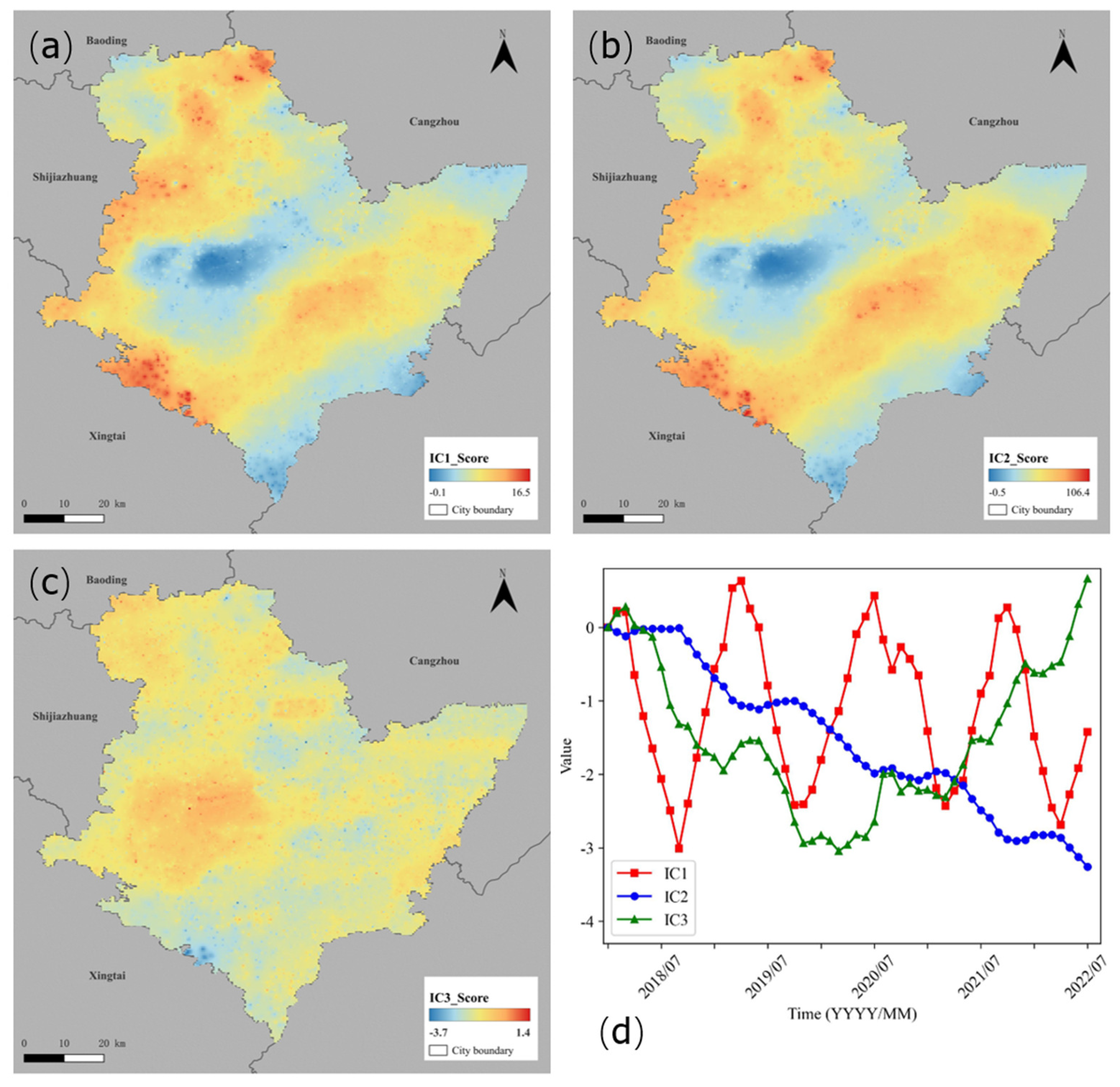
By performing independent component analysis (ICA) on the time series InSAR data, we extracted three independent components (IC1, IC2, and IC3), which represent different features of surface deformation: seasonal features (IC1), trend features (IC2), and random features (IC3). The analysis results showed that the time series of IC1 (seasonal feature) exhibited obvious cyclic fluctuation with a spatial score ranging from −0.1 to 16.5 (Figure 3a), and this seasonal deformation may be closely related to the fluctuation of the hydraulic head and variations in precipitation, reflecting the influence of cyclic natural processes; the time series of IC2 (trending feature) exhibited a continuous downward trend with a spatial score ranging from −0.5 to 106.4 (Figure 3b), and this deformation trend may be related to anthropogenic activities such as the long-term over-exploitation of groundwater and stratum compression; the IC3 (stochastic feature) time series fluctuations decreased and then rose, with spatial scores ranging from −3.7 to 1.4 (Figure 3c), and this stochastic feature may have been caused by measurement noise, short-term surface activities, or other uncontrollable factors.

In addition, the spatial scores of IC1 and IC2 had a high degree of consistency in spatial distribution, indicating that there was a spatial coupling relationship between seasonal deformation and deformation trend, which further revealed the dual influence of groundwater overdraft on surface deformation (Figure 3d).

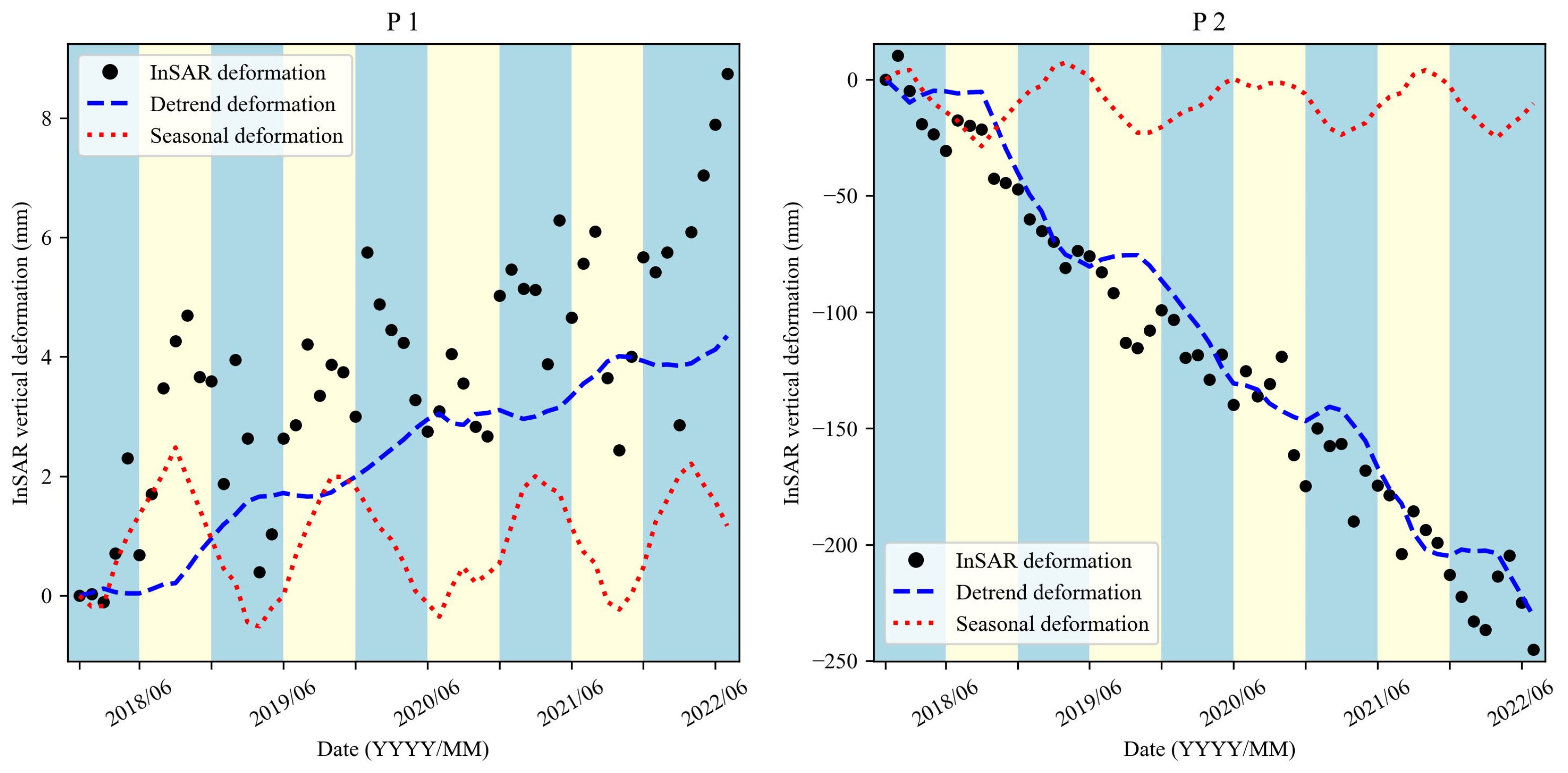
We successfully separated the trend component and seasonal component of the surface deformation through independent component analysis (ICA) of the time series InSAR data, and we selected one rebound point (P1) and one settlement point (P2) for analysis (Figure 4, location references in Figure 2). From the InSAR time series data of point P1, the point showed smoother positive fluctuations with a maximum rebound value of +8.74 mm, indicating that the ground experienced a certain degree of recovery during the study period (Figure 4a). Through ICA separation, the trending deformation time series data showed a rebound trend of the rebound point, which was smaller in magnitude but still exhibited the characteristics of seasonal fluctuation. The seasonal time series data, on the other hand, reflected significant cyclic variations, especially in spring and summer, when the ground recovery of this rebound point was more obvious. For point P2, the InSAR time series data showed a continuous trend of increasing deformation values at this point, with a maximum subsidence of −245.2 mm, indicating that land subsidence continued to deepen during the study period (Figure 4b).

4.3. Surface Deformation Caused by Hydraulic Head Changes

In order to study the correlation between the hydraulic head and surface deformation, we selected four typical water level monitoring wells to analyze the relationship between hydraulic head changes and the deformation trend, as well as seasonal deformation.

4.3.1. Relationship Between Seasonal Deformation and Seasonal Hydraulic Head Changes

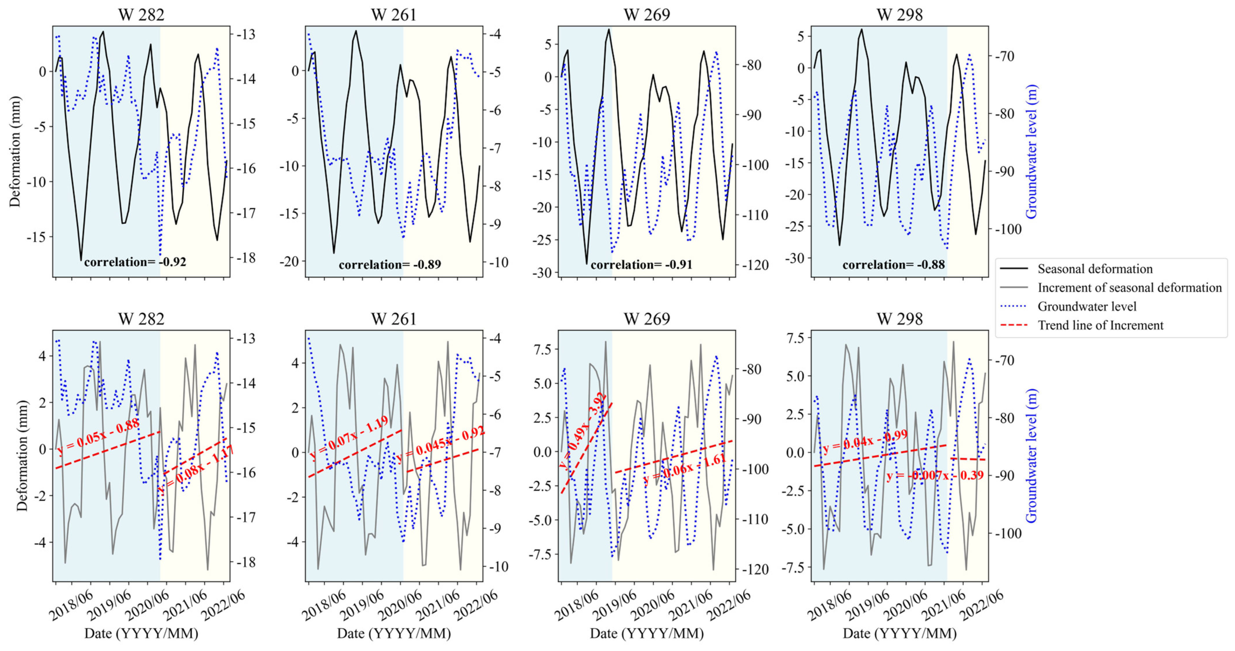
By analyzing the seasonal deformation and hydraulic head time series data at the four water level points in the study area, it was found that the amplitude of the seasonal deformation at the four water level points showed obvious cyclical fluctuations in different time periods (Figure 5). The range of the amplitude of deformation was from −26.31 mm to 5.30 mm, which indicated that there was a significant seasonal rise and fall of the ground surface in the study area, and the increment of seasonal deformation showed an overall upward trend. This phenomenon indicated that seasonal changes in the hydraulic head have a significant effect on ground deformation.

Figure 5 shows that the fluctuating trend of deformation was highly consistent with the trend of hydraulic head changes. In particular, the magnitude of land subsidence increased significantly during the period of the decreasing hydraulic head, while the magnitude of land subsidence decreased during the period of a rebounding water level. This trend suggested that seasonal fluctuations in the hydraulic heads drove the cyclical changes in land subsidence to some extent, and that declining hydraulic heads may exacerbate the rate of land subsidence.

In order to further quantify the relationship between seasonal deformation and hydraulic head changes, correlation analyses between the deformation magnitude and the hydraulic head magnitude were performed in this study. The results showed that the correlation coefficients between the deformation amplitude and the hydraulic head change amplitude at the four water level points were high, with values of −0.92, −0.89, −0.91, and −0.88, respectively, and all the correlation coefficients were significantly negative, which indicated that there was a significant negative correlation between the two. Specifically, the magnitude of land subsidence increased when the hydraulic head decreased, while the magnitude of land subsidence decreased when the hydraulic head rebounded. This negative correlation reflected the direct effect of the hydraulic head changes on land subsidence: when the water level drops, groundwater loss leads to compaction and consolidation of the soil layer, which leads to land subsidence; while, when the water level rises, groundwater recharge may ease the compaction of the soil layer, which slows down the rate of land subsidence.

It is worth noting that although this study found a strong negative correlation between seasonal deformation and groundwater fluctuations (r = −0.88 to −0.92), such correlation may only reflect the short-term direct hydraulic response mechanism, without fully accounting for the contribution of groundwater fluctuations to long-term subsidence. As emphasized by Akitaya and Aichi (2023) in their research on aquifer system deformation, seasonal groundwater level changes may exert sustained influence on long-term cumulative deformation through pore pressure diffusion and time-delayed plastic deformation of the soil matrix [53]. This is consistent with the findings of Yang Jilong et al. (2019) in the coastal area of Tianjin, who concluded that even after removing the long-term trend component, seasonal water level fluctuations could still explain approximately 23% of the variance in long-term land subsidence [54].

4.3.2. Relationship Between the Deformation Trend and the Trend of Hydraulic Head Changes

By analyzing the time series data for the deformation trend and hydraulic head trends at the four water level points in the study area, it was found that there was a significant correlation between the deformation trend and the trend in hydraulic head changes. The deformation trend magnitude and the trend for the water level change magnitude showed significant synchronization at different time periods, especially during the period of continuous hydraulic head decline; the deformation trend also showed a corresponding subsidence trend (Figure 6). This phenomenon indicated that there is a close relationship between the seasonal changes in the hydraulic head and ground deformation, and this relationship shows a certain regularity.

Based on the trend of hydraulic head changes observed at the four monitoring wells in Figure 6, it can be seen that the water level at the other three points showed an upward trend, except for point W282, which showed a downward trend. Although the trend’s cumulative deformation volume at the four points continued to increase, the deformation increment showed a decreasing trend. This phenomenon may indicate that although changes in the hydraulic head continue to affect surface deformation, the magnitude of fluctuations in the hydraulic head gradually leveled off over time, resulting in a slower deformation rate.

In order to further quantify the relationship between the deformation trend and the trend of hydraulic head changes, correlation analyses of the deformation magnitude and the water level magnitude were conducted in this study. The correlation coefficients at the four monitoring wells were −0.94, −0.91, −0.93, and −0.92, respectively, indicating a significant negative correlation. Specifically, as the hydraulic heads declined, the deformation amplitude increased; conversely, when the hydraulic heads rose, deformation amplitude decreased.

It is particularly important to highlight that the high correlation coefficients between the trend-type deformation and the groundwater level variation (r = 0.84–0.89) may in fact reflect the superposition of two distinct mechanisms: one being the irreversible compaction caused by prolonged groundwater overexploitation (Li et al., 2023), and the other being the gradual accumulation resulting from the compression of aquitards driven by seasonal fluctuations in the hydraulic head [8]. This can help explain the continued increase in the trend-type deformation after October 2020 (see well W282 in Figure 6), despite an observed rebound in groundwater levels. This phenomenon aligns with the “compression lag effect” proposed by Yang Jilong et al. (2019) [54], which posits that aquifer systems subjected to long-term depletion may require several years to complete pore pressure dissipation and structural adjustment of the sediment matrix.

4.4. Time Lag Correlation Between Surface Deformation and Hydraulic Head

In this study, the time lag relationship between land subsidence and the hydraulic head was investigated by analyzing the correlation between the InSAR land subsidence time series data and the hydraulic head time series data at 16 water level points. The results showed that there was a significant time lag effect between the land subsidence and the hydraulic head changes, and the deformation of different time scales (primitive, seasonal, and trending) had different lag times and correlation strengths with the water level changes.

Figure 7 demonstrates the maximum correlation coefficients between the original, seasonal, and trending deformations and the hydraulic head and their lag times. The X-axis indicates the water level point number, and the Y-axis indicates the correlation coefficients. According to Figure 7, the maximum correlation coefficients between the raw InSAR deformations and the hydraulic heads were generally high, ranging from 0.83 to 0.90. These high correlation coefficients indicated that there was a significant correlation between land subsidence and changes in the hydraulic heads in the raw time series data. The short lag time, which is 0 or 3 months for most of the hydraulic head points, indicated that changes in the groundwater table had a rapid effect on land subsidence. The maximum correlation coefficients between seasonal deformation and the seasonal hydraulic head were generally consistent, with the highest correlation coefficient at 0.76 and the lowest at 0.70, which indicated that seasonal groundwater table changes had a stable effect on seasonal land subsidence. Most of the lag time was from 0 to 4 months, which indicated that the seasonal water level changes had a rapid effect on seasonal deformation. The maximum correlation coefficients between the deformation trend and the trend of hydraulic head were generally high, ranging from 0.84 to 0.89, with most points having correlation coefficients close to 0.85, which was further evidence of the long-term effect of the trend of hydraulic head changes on trend land subsidence. The lag times are generally long, ranging from 0 to 12 months, suggesting that there was some time delay in the effect of trending hydraulic head changes on the trending deformation. These findings suggested that the effects of hydraulic head changes on land subsidence are time-lagged and cumulative, and that deformations at different time scales have different response mechanisms to water level changes.

4.5. Estimation of the Water Storage Coefficient of the Aquifer System Skeleton

By analyzing the deformation and hydraulic head variation at 16 monitoring points within the study area, significant differences between the aquifer and aquitard deformation behaviors were identified (Figure 8). The results suggested a stratified mechanism underlying land subsidence: elastic deformation in aquifers and elastoplastic deformation in aquitards operate simultaneously but exhibit fundamentally different spatiotemporal responses.

The spatial distribution of the elastic skeletal specific storage coefficient (Ske) showed high values (up to 9.51 × 10⁻³) concentrated in the unconsolidated sediment zones of the northwest and southeast, indicating the strong elastic water release capacity of the sand-gravel aquifers under short-term fluctuations in the hydraulic head. This deformation was largely reversible, and could partially recover when groundwater levels rose (Figure 8a). This behavior is consistent with Terzaghi’s effective stress principle, in which the elastic compression of sand–gravel aquifers corresponds to the instantaneous dissipation of pore water pressure (Δσ′ = Δu), resulting in a linear relationship between deformation and water level changes.

In contrast, the spatial distribution of the inelastic skeletal specific storage coefficient (Skv) indicated that the central alluvial fan zone, characterized by clay-rich lenticular aquitards (Skv = 3.97 × 10⁻³), exhibited more pronounced irreversible deformation. According to Biot’s consolidation theory, plastic deformation in clay layers results from particle rearrangement under sustained increases in effective stress (Figure 8b). When water levels decline, although aquifer elasticity dominates the short-term deformation response, pore pressure diffusion in aquitards proceeds three to five times slower than in sand–gravel layers (Yang Jilong et al., 2019), leaving the clay-rich strata in a state of excess pore pressure for extended periods, ultimately triggering irreversible compaction [54]. This mechanism suggests that the non-recoverable component of land subsidence is primarily attributable to plastic deformation within the aquitards.

5. Discussion

This study integrated persistent scatterer interferometric synthetic aperture radar (PS-InSAR) and independent component analysis (ICA) to systematically monitor and analyze the ground deformation in Hengshui City from January 2018 to 29 July 2022, based on Sentinel-1A SAR data. The InSAR time series results revealed multiple subsidence centers and clearly exhibited the spatiotemporal evolution of surface deformation. Long-term subsidence was primarily concentrated in the central and southern parts of the study area, where prolonged overexploitation of groundwater had led to a continuous decline in the hydraulic head, exceeding the pre-consolidation stress threshold of the aquitards. This triggered inelastic skeletal compaction and resulted in irreversible land subsidence. The spatial distribution of subsidence closely corresponds to the areas of intensive agricultural irrigation and urban water consumption, highlighting long-term anthropogenic hydraulic stress as the dominant driver of regional deformation trends.

A comparative analysis between the cumulative displacement retrieved from InSAR and the observed values from borehole extensometers revealed a stage-dependent deviation. Specifically, during the early phase characterized by relatively small displacements, InSAR estimates tended to exceed those measured by borehole extensometers. In contrast, during the later phase when displacements were larger, InSAR consistently underestimated the deformation. This discrepancy may stem from several technical and physical factors. InSAR deformation is obtained through the accumulation of multitemporal interferometric phase data, which are susceptible to short-term atmospheric disturbances and nonlinear deformation signals. In the early monitoring period of this study, the dominant driving mechanism was the discharge of shallow groundwater. The millimeter-scale vertical fluctuation signals during this stage partly overlapped with the frequency characteristics of atmospheric noise, potentially leading to systematic overestimation of displacements, even after filtering. Furthermore, when the deformation exceeds a certain threshold, the PS-InSAR algorithm becomes sensitive to the temporal baseline length. In cases of long-term subsidence, the accumulation of phase unwrapping errors may occur. Once the actual deformation rate surpasses the phase unwrapping tolerance threshold of the Sentinel-1 revisit interval (12 days), the algorithm may fail to fully recover the total displacement, resulting in underestimation. In contrast, borehole extensometers, which directly measure the subsurface vertical movement, maintain higher fidelity in capturing nonlinear and large-magnitude deformations.

Using ICA, the InSAR time series was decomposed into seasonal (IC1), long-term trend (IC2), and random (IC3) components. The seasonal deformation component was highly correlated with fluctuations in the hydraulic head, exhibiting a clear periodicity that confirmed the short-term elastic response of the surface deformation to seasonal groundwater variation. The long-term trend component reflected the progressive compaction of strata induced by sustained groundwater depletion and presented an irreversible and cumulative nature. The application of ICA effectively separated multiple deformation sources, enhanced interpretation accuracy, and significantly suppressed random noise in the time series data, thereby clarifying the dominant deformation mechanisms.

A study by Li et al. (2023), based on RADARSAT-2 data and SBAS-InSAR, also reported that subsidence areas in Hengshui coincided with intensive groundwater extraction zones [8]. Despite a partial recovery in groundwater levels after 2019, their results showed that the subsidence rate did not significantly decrease, which was attributed to the delayed compaction of compressible strata. The present study further suggested that this phenomenon may be related to the formation of a new pre-consolidation head following prolonged drawdown, indicating that aquitard compression may persist even after the hydraulic head recovers, thereby reinforcing the cumulative nature of subsidence.

By integrating InSAR-derived deformation with hydrological data, this study further quantified the influence of groundwater level variations on land subsidence. In the short term, groundwater fluctuations induced a rapid response in surface deformation, with lag times of 0–4 months, reflecting a strong seasonal modulation effect. In contrast, at the long-term scale, trend-type subsidence was more strongly correlated with the decline in the hydraulic head (correlation coefficient r = 0.84–0.89), with a lag time of up to 12 months, suggesting that compaction processes under long-term depletion exhibit significant hysteresis. This finding indicated that prolonged groundwater extraction caused irreversible changes in the aquifer system, where cumulative compaction further reduced storage capacity. Li et al. (2023) attributed variations in the subsidence lag time to the compressibility of Quaternary sediments in Hengshui [8]. The present study supports this hypothesis and emphasizes the critical role of the rate of hydraulic head decline in controlling long-term deformation trends.

It is worth noting that the attribution of long-term subsidence in this study may be somewhat simplified. According to the dual-process model proposed by Akitaya and Aichi (2023), trend-type subsidence consists of (1) transient responses synchronous with groundwater level changes, and (2) residual deformation accumulated from historical overexploitation, which is independent of current water level variations [53]. The high correlation coefficients (r = 0.84–0.89) in this study may have overestimated the contribution of the transient component while underestimating the impact of residual compaction. This could help explain the non-monotonic relationship between the groundwater level recovery and the subsidence rate observed by Li et al. (2023), which likely resulted from the superposition of deformation processes operating at different temporal scales [8].

PS-InSAR provides high-precision and wide-area monitoring capabilities for land subsidence, offering valuable support for groundwater resource management and subsidence mitigation. However, the spatial resolution of PS points is limited in rural or vegetated regions, which constrains the detection of localized subsidence hotspots. Additionally, the limited number of groundwater observation wells may affect the ability to accurately model the groundwater–subsidence relationship. Future research could incorporate higher-resolution remote sensing data (e.g., GRACE gravimetric data) and in-situ monitoring to improve deformation detection and temporal responsiveness. Furthermore, hydrogeological numerical models (e.g., MODFLOW) could be employed to simulate groundwater–deformation interactions, thereby optimizing regional groundwater management strategies. In combination with climate variability and precipitation trends, long-term evaluations of groundwater evolution and its impact on land subsidence are essential to support sustainable water resource management.

6. Conclusions

In this paper, in response to the problems with a small number of data points, small spatial coverage, and the lack of in-depth research on the influencing factors of subsidence features in the separation of large-scale land subsidence features in the North China Plain, we took Hengshui City as the study area, combined the InSAR land subsidence time series data with the independent component analysis (ICA) method, carried out a systematic analysis of the subsidence features and their main controlling factors, and further estimated the changes in groundwater storage. The research results showed as follows:

(1) The subsidence phenomenon in Hengshui is remarkable, with the maximum amount of subsidence reaching 417.05 mm, and its spatial distribution is mainly concentrated in the Shenzhou and Raoyang counties in the northwest and the Jing and Zaoqiang counties in the southeast; the subsidence is closely related to changes in the hydraulic head, especially during the period of declining water levels, where the magnitude of land subsidence was significantly increased.

(2) The land subsidence in Hengshui City is mainly characterized by three features, namely seasonal features (IC1), trend features (IC2), and stochastic features (IC3), reflecting different subsidence characteristics and their driving mechanisms.

The results of the ICA analyses showed a close correlation between seasonal deformation (IC1) and hydraulic head fluctuations, with the time series data showing periodic changes. During spring and summer, the rebound of the hydraulic head led to a ground rebound, while autumn and winter were periods of declining hydraulic heads with increased land subsidence. This result verified the influence of seasonal changes in the hydraulic head on land subsidence, suggesting that hydraulic head fluctuations are the main driver of cyclical changes in land subsidence.

The deformation trend (IC2) revealed the persistent effect of the long-term over-exploitation of groundwater on land subsidence, which manifested in the gradual deepening of the subsidence amplitude. As the long-term over-exploitation of groundwater leads to stratum compaction, intensifies land subsidence, and presents irreversible characteristics, and the subsidence area was highly consistent with the high-intensity groundwater mining area, indicating that the long-term over-exploitation of groundwater was the dominant factor for land subsidence in Hengshui City.

(3) The influence of hydraulic head changes on land subsidence had a significant time lag effect, and different response mechanisms in different time scales revealed the complex influence of groundwater changes on the land subsidence in Hengshui.

In the short term, the high correlation (0.83 to 0.90) and the short lag time (0 to 3 months) between the original deformation and the hydraulic head changes indicated that the hydraulic head changes had a more direct and rapid influence on land subsidence. In particular, dynamic changes in the hydraulic head during pumping and recharge caused an immediate subsidence response, and this effect would be more pronounced in areas with a higher intensity of groundwater extraction. In addition, the correlation between seasonal deformation and hydraulic head fluctuations showed a stable time lag effect, with correlation coefficients ranging from 0.70 to 0.76, and lag times ranging from 0 to 4 months. This indicated that the fluctuation of the hydraulic head due to precipitation and seasonal mining had a continuous and stable effect on subsidence in the short term, and the cyclic rise and fall in the water level accompanied by synchronization with the change in the magnitude of land subsidence reflected the cyclic regulating effect of hydraulic head changes on land subsidence.

In the long term, the correlation between the deformation trend and long-term changes in the hydraulic head was stronger (0.84 to 0.89), but with a longer lag time (0 to 12 months), suggesting that there was a significant delay in the effect of ground compaction and the intensification of subsidence triggered by a long-term decline in groundwater, and that the long-term over-exploitation of groundwater led to a reduction in groundwater storage and compaction of the ground surface, resulting in the continual deepening of irreversible land subsidence.

(4) Based on the analysis of shape variables and the amount of hydraulic head changes at the 16 monitoring points, the results showed that there were significant spatial differences in both the elastic skeleton water release coefficient (Ske) and the inelastic skeleton water release coefficient (Skv) in the Hengshui area.

The elastic skeleton water release coefficient (Ske) varied from 0.42 × 10⁻³ to 9.51 × 10⁻³, with high values concentrated in the northwestern and southeastern regions, indicating that the aquifers in these regions had a strong elastic water release capacity and that the hydraulic head fluctuations significantly affected land subsidence. The lower Ske values in the central part of the region reflected its weak elastic water release capacity, and the hydraulic head changes had less influence on subsidence. This difference could be attributed to the differences in geological structure within the region, with thicker sedimentary layers and large hydraulic head fluctuations in the northwest and southeast, and dense rock layers and relatively stable hydraulic heads in the central part of the region, leading to the spatial differentiation of elastic water release capacity.

The variation of the inelastic skeletal water release coefficient (Skv) ranged from 3.94 × 10⁻³ to 129.84 × 10⁻³, and the overall distribution trend was similar to that of the Ske coefficient, showing obvious spatial differences. The higher values of Skv in the northwest and southeast indicated that the inelastic water release capacity was higher in these regions, and the compaction effect of the strata triggered by the decline of the hydraulic head was significant, leading to the increase in land subsidence. These results suggest that the region is characterized by a thick unconsolidated sedimentary layer with high clay content and strong compressibility. Coupled with pronounced groundwater fluctuations, long-term overexploitation has significantly enhanced the compaction and consolidation of the aquifer system. This has intensified plastic deformation, continuously reduced the aquifer’s storage capacity, and ultimately led to irreversible degradation of the regional groundwater system. In contrast, the lower value of Skv in the central region indicated that its inelastic water release capacity was weaker, the stratum was denser, the sedimentary layer was thinner, the particles were coarser, the groundwater fluctuation was smaller, and the subsidence amplitude was limited.