Study on the Risk of Urban Population Exposure to Waterlogging in Huang-Huai Area Based on Machine Learning Simulation Analysis—A Case Study of Xuzhou Urban Area

Abstract

With the acceleration of climate change and the increase of extreme rainfall, the risk of flooding has intensified in the Huang-Huai region, which is often hit by floods. Urban water accumulation is a complicated process, and the hydrological simulation analysis is highly accurate, but it is time-consuming and laborious. Machine learning is becoming an important new method because of its ability to analyze large areas with high precision. In this paper, a simulation analysis method based on machine learning is constructed by selecting 13 disaster factors, and the waterlogging point in Xuzhou city is predicted successfully. The following conclusions are found: (1) Among the five machine learning models, CatBoost has the highest accuracy rate, reaching 81.67%. (2) Temperature, elevation, and rainfall are relatively important influencing factors of waterlogging. (3) Machine learning can discover water accumulation areas that are easily overlooked except for the built-up areas. (4) The results of the coupling analysis show that the exposure risk of the population exposed to rainwater in the old urban area, the southern area, and the northwestern area is relatively high. This research is of great significance for reducing the risk of exposure to rain and flooding and promoting the safety and sustainable development of cities.

1. Introduction

With the improvement of China’s infrastructure construction, the level of response to flood and waterlogging risk has been improved, and the population and property losses caused by flood have been significantly reduced. However, compared with Germany, Japan, and other countries, the proportion of population and economic losses caused by rain and flooding is still high [1]. The sixth report of the United Nations Intergovernmental Panel on Climate Change pointed out that 9 of the 15 extreme tipping points of climate change have been exceeded, and the risk of flooding has increased worldwide [2]. In recent years, China’s 800 mm iso-precipitation line has a northward trend, and rainfall in the north has begun to increase. However, the level of prevention and control of rainlogging in the north is relatively low, which greatly increases the uncertainty and harm of future rainlogging risk [3]. The results show that the increase in the extreme precipitation index will be the most significant by the end of this century. Among them, the extreme precipitation index shows a significant increasing trend in Central China and Northeast China. The total annual precipitation shows an increasing trend in Central China and North China [4]. According to the study of Yu Kongjian, the risk of rain and waterlogging in Huang-Huai region is at a high level in China due to flat terrain and dense population [5]. The causes of urban flooding also include urbanization, climate change, land use, and ecology. In particular, the local microclimate formed by urban heat islands can also affect rainfall and urban flooding [6]. Although China has also put forward measures to strengthen the construction of old urban areas, improve the drainage capacity, construct sponge cities and resilient cities, and other suggestions, the guidance of the overall policy for specific cases is still weak. For instance, large-scale fatal accidents caused by floods still occurred in Beijing and Zhengzhou [7].

At present, the main research methods for assessing the risk of rain and waterlogging involve simulating runoff using SWMM [8], HAC-RAS [9], SWAT [10], and other software. These simulation methods are capable of producing high-precision numerical results. However, numerical model simulations for large-scale areas with complex underlying surfaces are complicated and time-consuming. This makes it difficult to meet the aging requirements of rainstorm waterlogging and waterlogging prediction, while also significantly decreasing accuracy [11]. However, the advantages of machine learning methods that can handle large amounts of data and require low data accuracy are very obvious [12]. AI has a flexible mathematical structure and can simulate the complex nonlinear relationship between the input and output data features. This is difficult to describe using physical equations in hydrodynamic simulation research [13]. The use of AI technology for disaster prevention and early warning is a new trend in recent years [14]. For example, convolutional neural network (CNN) technology can be applied to deal with urban waterlogging [15], CNN technology is most commonly used in image processing; Artificial neural network (ANN) is one of the most widely used technologies in artificial intelligence flood forecasting in the world. Although ANN is prone to overfitting, it has a strong ability to analyze and process the results of linear data, which can be used for predicting the depth of water accumulation. They simulate the brain’s problem-solving function through mathematical models inspired by neural processes [16,17]. Scholars have gradually applied machine learning methods to the prediction of rainstorm and waterlogging disasters. Machine learning methods include lasso regression [18], SVM [19], decision trees, random forests [20], extreme gradient boosting (XGBoost) [21], and deep learning based on artificial neural networks [22]. Some machine learning models have similar counting principles, and their advantages and disadvantages can only be determined by comparing the simulation results. The learning characteristic factors include rainstorm intensity, rainfall duration, impervious rate, elevation, slope, topographic humidity index, distance from road, and drainage network density [23,24]. However, many relevant researches are used to put both disaster factors and disaster victims in the analysis of rain and waterlogging factors for machine learning simulation analysis [25]. This is unreasonable to some extent, as the occurrence of waterlogging is an objective cause. Meanwhile, people, land, and buildings, as disaster-bearing bodies, are not the direct cause of waterlogging. The real-time dynamics of the current research data are relatively low, and the reliance on historical disaster data is high. Therefore, there may be insufficient adaptability of the model to extreme rainfall.

People are the participants of urban economic development and the object of urban service. Together, they constitute the foundation and main body of social production behavior [26]. On the one hand, the acceleration of China’s urbanization process has led to the rapid expansion of urban population areas. On the other hand, it also intensifies the contradiction between population, resources, and environment [27]. Human life safety is the most obvious disaster-bearing body, so the analysis of population distribution is a very important content in the study of exposure risk of flood and waterlogging [28].With the rapid development of remote sensing technology, night light data—capturing varying light intensities generated by cities, small-scale residential areas, and traffic flows—has become an effective indicator for monitoring human activities [29,30]. At present, this technology is widely used in urban and rural population distribution, disaster population statistics, and other fields [31]. It uses brightness value to characterize the intensity of human activities. Related studies include socio-economic parameters, urban construction [32], natural disasters, resources, and environment, etc., and can be used as a proxy variable for a variety of social and economic indicators [33].

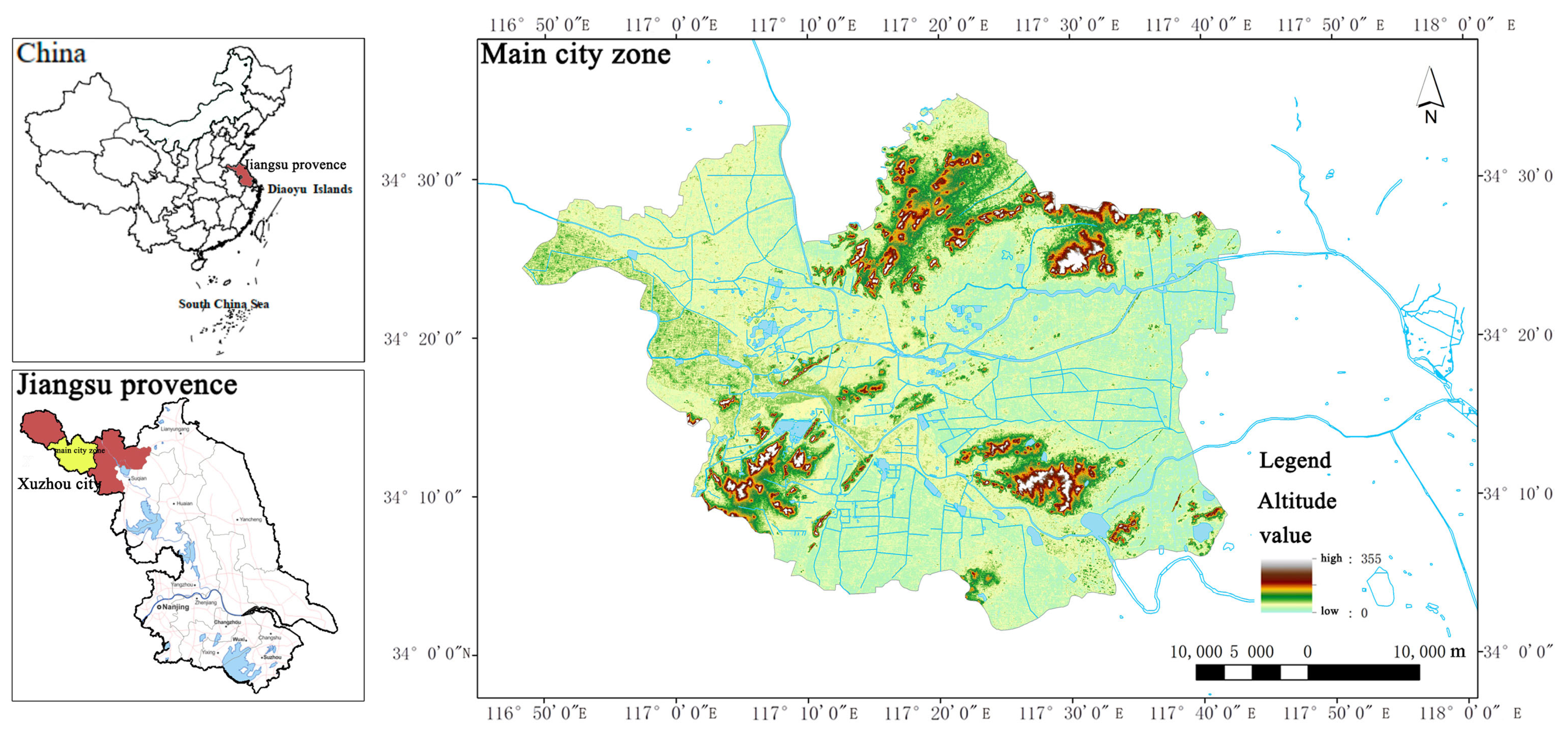
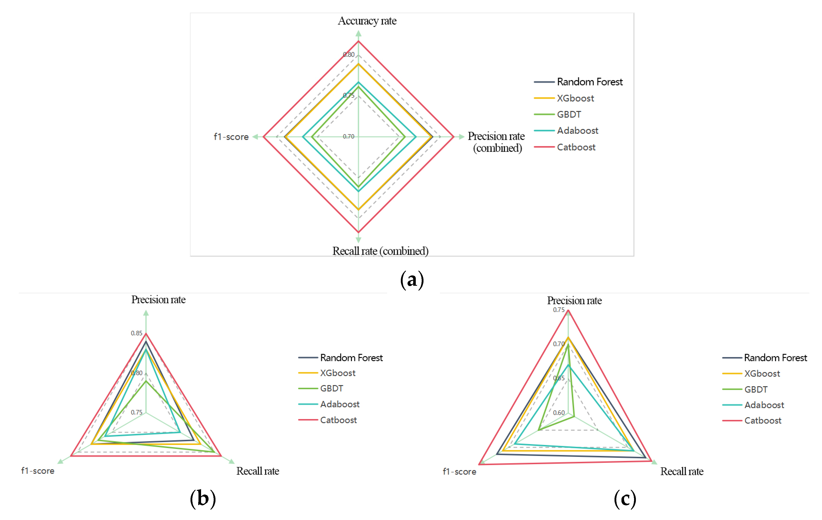
Therefore, this paper constructs a machine learning index system suitable for the assessment of rain and waterlogging in Huang-Huai region. Waterlogged and non-waterlogged were used as identification features. Five machine learning models were selected for verification. By comparing four indicators of machine learning output—accuracy rate, precision rate, recall rate, and F1-score—CatBoost demonstrated the best simulation effect. After that, nuclear density analysis was performed on the accumulation point area output by CatBoost model to obtain the accumulation risk level. The population distribution density is also analyzed based on the remote sensing light data at night. The result of waterlogging risk exposure can be obtained by coupling analysis of the two. We believe that this is of great benefit to guiding urban waterlogging control and promoting urban sustainable development of Xuzhou city in Huang-Huai area.

2. Materials and Methods

2.1. Introduction of Study Area

Xuzhou is located in the northwest of Jiangsu Province, in the southeast of the North China Plain, and on the north wing of the Yangtze River Delta. Its geographical coordinates are 116°22′–118°40′ east longitude and 33°43′–34°58′ north latitude. It is an important hub city at the border of Jiangsu, Shandong, Henan, and Anhui provinces. This study covers the main urban area of Xuzhou, which is dominated by plains (about 90%) and is part of the Huang-Huai Plain. The overall terrain of the main city slopes from northwest to southeast, and the elevation is mostly between 20–50 m (Figure 1). Low and flat terrain can easily lead to poor drainage during heavy rainfall. In addition, there are a small number of hills in the northeast, southwest, and east of Xuzhou (about 10%) [34]. The hills are an extension of the low hills in central and southern Shandong Province, with an elevation of 100–300 m. Although the topography is relatively undulating, it may still cause local flash floods or waterlogging during heavy rains.

As an important transportation hub in the country, Xuzhou is interwoven with railways, highways, and waterways, and the dense infrastructure may cause interference to the natural drainage path. The main city water system belongs to the waste Yellow River system, and the Beijing-Hangzhou Grand Canal runs through the north and south of the city. The river in the city is dense and connected to Weishan Lake, forming a complex water network structure [35]. The Yellow River has been rerouted through Xuzhou many times in history, leaving behind the abandoned Yellow River and becoming a regional watershed, but also causing some of the channel to silt up, increasing the risk of waterlogging in low-lying areas. Waterlogging prone areas in urban areas include the yellow flood plain and areas with weak drainage systems in the old city, especially the depression because of the low terrain and limited drainage capacity of the river, which is prone to water disaster in the rainstorm.

From the perspective of climate, Xuzhou is located in the subtropical monsoon area, belonging to the temperate monsoon climate type, and its climate characteristics are mainly manifested as abundant summer rainfall [36]. The rainfall in Xuzhou is mainly concentrated in June–September. Therefore, the precipitation and the disaster statistics of Xuzhou in these four months are carried out, and vectorization transformation is carried out in Arcgis.

2.2. Selection and Source of Disaster-Causing Factors

The selection of disaster factors should follow the principle of “scientific, quantifiable, and operational”, and should be dynamically adjusted according to regional characteristics. For example, plain cities focus on topography and drainage capacity, while mountain areas require additional consideration of flash floods and debris flow risks. According to the current main studies, it can be found that the selection of disaster-causing factors for risk assessment should comprehensively consider meteorological [37], terrain [38], natural, and artificial surface [39], and other multi-dimensional factors. In the process, the availability of actual data and the applicability of the model should be combined. Thirteen disaster factors are selected in this paper. The meteorological factors mainly include rainfall, temperature, and wind speed. The terrain mainly has three indexes: elevation, slope, and slope direction. The natural land surface mainly has three indexes: vegetation coverage, river network density, and surface humidity. Human activities will cause changes in the surface environment, so the artificial surface environment index includes land use, pipe network density, road density [40], and railway network density. The sources and addresses for obtaining data for the indicators are shown in

Table 1. Disaster Factors and Data Sources.

Factors	Data Sources	Address
Rainfall, temperature, wind speed	Ground-based basic meteorological observations in China	http://data.cma.cn/data/detail/dataCode/A.0012.0001.html (accessed on 1 October 2024)
Elevation, slope, slope direction, topographic wetness index	ASTER GDEM aster gdem 30 m	http://www.gscloud.cn/sources/accessdata/310?pid=302 (accessed on 1 October 2024)
	Topographic mapping data of Xuzhou urban area	Xuzhou Survey and Mapping Research Institute
Vegetation cover, land use	Landsat 8-9 OLI/TIRS C2 L1	https://www.usgs.gov/ (accessed on 1 October 2024)
River network density	Electronic map of the Water Classic	http://www.rivermap.cn/ (accessed on 1 October 2024)
Stormwater network density	Xuzhou City Drainage Network Data	Xuzhou Municipal Water Affairs Bureau
Road network density	Xuzhou road dataset	http://download.openstreetmap.fr/extracts/asia/china/ (accessed on 1 October 2024)
Railroad network density	Electronic map of the Water Classic	http://www.rivermap.cn/ (accessed on 1 October 2024)
waterlogging point	Xuzhou urban areas vulnerable to waterlogging points responsibility list	Xuzhou Municipal Water Affairs Bureau
	Rainy season research data	https://www.wjx.cn/vm/tOVTTHo.aspx (accessed on 1 October 2024)
population density	NPP VIIRS Remote Sensing Data for Nighttime Lighting	https://payneinstitute.mines.edu/eog/nighttime-lights/ (accessed on 1 October 2024)
	Xuzhou Township Population Statistics	https://www.xzqhdm.cn/detail/2104291053446663 (accessed on 1 October 2024)

.

The formation of rain and waterlogging disasters is affected by multiple factors. In terms of climate, rainfall intensity and duration directly determine the surface runoff and drainage load, which is the core factor of inducing disasters [41]. Temperature changes indirectly affect surface water infiltration and runoff generation by regulating evaporation, precipitation pattern (rain and snow conversion), and soil moisture. Strong winds may accelerate evaporation or promote storm cloud formation, thereby altering precipitation distribution. In topographic conditions, elevation difference controls hydrodynamic characteristics. High altitude water flow rates can easily cause flash floods, while low-lying areas are prone to waterlogging. Slope is closely related to disaster type. Steep slopes increase the risk of landslides due to runoff erosion, while gentle slopes increase the probability of waterlogging due to poor drainage [42]. Slope direction changes local hydrological processes by regulating sunshine intensity. The positive slope has strong evaporation and dry surface, while the negative slope is more prone to persistent water formation. In terms of land cover characteristics, the high vegetation cover area can trap 20–40% of rainfall [43], significantly reducing the peak runoff. The risk of waterlogging can be reduced in areas with high river network density due to perfect drainage channels [44], while the runoff coefficient in urban areas with large proportion of hardened land surface is many times higher than that in rural areas. Soil moisture directly affects the infiltration capacity, and the proportion of surface runoff transformed by rainfall with high saturation is very high [45]. Human activities have profoundly altered hydrological response mechanisms. Urbanization increases the proportion of impervious surfaces, which leads to an increase in runoff coefficient. With the increase of drainage network density, the probability of waterlogging can decrease significantly [46]. New catchment units created by the construction of the traffic network (such as the tunnel) can change the natural catchment path, and the risk of waterlogging is many times higher than that of ordinary roads [47]. The spatio-temporal coupling of these factors together determines the disaster mechanism and risk level of rain and waterlogging disasters.

2.3. Analysis of Disaster-Causing Factors

2.3.1. Meteorological Factor Analysis

Depending on the latitude and longitude of the weather station, the excel data table in Arcgis can be imported. By specifying the X field as longitude and the Y field as latitude, the weather station points can be loaded into Arcgis 10.2. By connecting the original table, the file attribute table can be loaded. By exporting a new layer through layers, a new point file of the weather station can be obtained, which can be converted from GCS_WGS_1984 to CGCS_2000_3_Degree_GK_Zone_39 by defining the coordinates and coordinate projections. Figure 2a and Figure 2b respectively show the temperatures in the Huang-Huai region and the urban area of Xuzhou. The rainfall in regional and Xuzhou urban area are shown in Figure 2c and Figure 2d respectively; The results of wind speed are shown as Figure 2e and Figure 2f.

2.3.2. Terrain Factor Analysis

The elevation data used in the thesis comes from the GDEMV3 30 m resolution digital elevation data of the Geospatial Data Cloud Platform, which was released by NASA and METI of Japan on 5 August 2019, with a high degree of data accuracy, but it is found that the accuracy of this data decreases significantly in urban areas due to the influence of complex buildings. Therefore, the elevation data is corrected by mapping data of mosaic built-up areas to achieve the requirement of improving data accuracy (Figure 3a). The slope and slope direction of the elevation data are analyzed by Arcgis, and the slope analysis map (Figure 3b) and slope direction analysis map (Figure 3c) are obtained.

2.3.3. Natural Surface Factor Analysis

Land use data were downloaded from Landsat 8-9 OLI/TIRS C2 L1 satellite data via USGS. Classification and interpretation were done in ENVI 5.3 software after radiometric calibration and atmospheric radiation. The interpretation process was done by categorizing the land into seven types of land i.e., forest land, shrub, grassland, agricultural land, water, built-up land, and bare land. For each type of land, 30 areas were selected for identification and analysis by visual comparison, and the final results are shown in Figure 4a. There are a number of methods for measuring vegetation cover using remotely sensed data, and one of the more practical methods is the approximate estimation of vegetation cover using vegetation indices. In this paper, the remote sensing data used to study the vegetation cover are downloaded from Landsat 8-9 OLI/TIRS C2 L1 satellite data from the USGS. After radiometric calibration with atmospheric radiation, the vegetation index NDVI can be obtained by band calculation.

NDVI = (NIR − R)/(NIR + R)

(1)

where NDVI stands for the vegetation index and NIR and R are reflectance values at the near-infrared and red bands, respectively.

FVC = (NDVI − NDVIsoil)/(NDVIveg − NDVlsoil)

(2)

where FVC stands for vegetation cover, NDVIsoi1 is the NDVI value of an area that is completely bare soil or without vegetation cover, and NDVIveg represents the NDVI value of an image element that is completely covered by vegetation, i.e., the NDVI value of a purely vegetated image element. The formula for these two values is:

NDVlsoil = (FvCmax*NDVlmin − FvCmin*NDVlmax)/(FVCmax − FVCmin)

(3)

NDVlveg = ((1 − FVCmin)*NDVImax − (1 − FVCmax)*NDVlmin)/(FvCmax − FVCmin).

(4)

The key to calculating vegetation cover using this model is to calculate NDVIsoi and NDVlveg. There are two assumptions here:1) FVCmax = 100% and FVCmin = 0% can be approximated in the region.

Equation (2) can be changed to:

FVC = (NDVI − NDVImin)/(NDVImax − NDVlmin)

(5)

NDVImax and NDVImin are the maximum and minimum NDVI values in the region, respectively. Due to the inevitable presence of noise, NDVIveg and NDVIsoi1 are generally taken as the maximum and minimum values within a certain confidence range. The value of confidence is mainly based on the actual situation of the image, and in this study, the maximum and minimum values are replaced by the values of the first 5% and the last 5% based on general experience. Therefore, the corresponding maximum and minimum values are 0.670588 and −0.074510. The calculation formula for the input band in ENVI 5.3 software is:

(b1 lt − 0.074510)*0 + (b1 gt 0.670588)*1 + (b1 ge − 0.074510 and b1 le 0.670588)*((b1 + 0.074510)/(0.074510 + 0.670588))

(6)

In the above formula, b1 represents the NDVI value, and the operators represent the meaning of less than (lt), less than or equal to (le), greater than or equal to (ge), and greater than (gt), respectively.

Based on the above analysis process, the corresponding vegetation coverage can be obtained (Figure 4b). The vector data of the river network were downloaded from the Hydrosearch software V4.1.61. Statistical analysis of river network density was carried out by constructing fishing nets, and finally, the corresponding results were obtained (Figure 4c).

The Terrain Wetness Index (TWI) is an indicator that can reflect the degree of wetness of regional topography and is generally used in hydrology and ecology. The formula for calculating the terrain moisture index is shown below:

TWI = ln (a/tanβ)

(7)

where ‘a’ represents the specific catchment area (specific catchment area), which usually represents the area of the upstream watershed per unit width, in m²/m; and β represents the slope, expressed as the angle of inclination of the slope, in radians.

Specific catchment area (a) describes the potential for water to pool from upstream to a point, with larger values indicating that more water may pool at that point. Slope (β) reflects the potential for water loss; the steeper the slope, the faster water is lost. Thus, TWI combines the properties of water pooling and loss, with larger values indicating that the soil in the area is likely to be wetter. And the specific catchment area ‘a’ is expressed as:

a = A/w

(8)

where A represents the total catchment area of the confluence to a point (unit: m²); w represents the width of the confluence (unit: m), which is related to the size of the raster cell in the grid-like DEM. In this paper, the side length of the grid is 30 m. Because the digital elevation model (DEM) represents the topography in the form of a grid, the calculation of the specific catchment area needs to be carried out to calculate the flow direction and cumulative flow calculation.

Therefore, the elevation DEM data needs to be analyzed in Arcgis by filling and excavating first. After that, the fill-excavation data are used to analyze the flow direction. Then, flow analysis is performed based on the results of flow direction analysis. Then, the fill and excavation analysis data are used to calculate the slope, which is measured in degrees. After that, a raster calculator was used to convert the slope data into units to obtain new slope data in radians. The raster calculator was used to calculate the tan slope, and then the flow data was used for raster calculation to obtain the specific catchment area SCA, which was calculated by the formula (flow data + 1)/30. Finally, the raster calculator was used for the calculation of the ln function to obtain the topographic wetness index (TWI), and the results are shown in Figure 4d.

2.3.4. Artificial Surface Factor Analysis

The density of pipe network was obtained from Xuzhou Planning Bureau, and after vectorizing the data through Arcgis, the density calculation was carried out in the fishing network grid, and the results are shown in Figure 5a. The road network and railroad network density data are processed in the same way as the pipe network density. However, the data source of road network is from OMS, while the data source of railroad network is from the software of hydro-economic note. The analyzed results are shown in Figure 5b,c.

2.4. Introduction to the Technical Route

In this study, the rationality of the model was determined by collinearity analysis of 13 disaster-causing attribute data extracted from 899 hydrops and non-hydrops points. Then, five machine learning models were simulated and analyzed to determine the appropriate machine learning algorithm by accuracy, f1 score, recall rate, and other indicators. The waterlogging results obtained by the optimal algorithm were exported to Arcgis 10.2 software for kernel density calculation, and the risk level of waterlogging was determined. Then, the night light data and population data are regression analyzed to reflect the distribution density of the population. Finally, the coupling analysis of the risk level of rainlogging and population exposure risk is carried out to obtain the final result of the exposure risk of rainlogging and population. The entire technical route is shown in Figure 6.

2.5. Extracting the Attributes of the Causal Factors

According to the distribution location of waterlogged points in the urban area announced by Xuzhou Water Affairs Bureau, the waterlogged areas are vectorized in Arcgis. At the same time, the waterlogged and non-waterlogged point data of our own research are also imported into Arcgis and merged with the data of the Water Affairs Bureau. The new field is Y, the waterlogged point is recorded as 2, and the non-waterlogged point is recorded as 1. The raster data values corresponding to X1–X13 are extracted by the function of multi-value extraction to the point in Arcgis, which corresponds to the location of the point. There are 899 sets of data used for machine learning training and validation, including 357 sets of waterlogged point data and 542 sets of non-waterlogged point data. The ratio of training and validation sets is 4:1. The data used for prediction is obtained by constructing fishing nets. A total of 32,865 sets of data were obtained by numerical extraction of points with the causal factors after the fishing net was transferred to the points. The attribute data values of training data, validation data, and analyzed prediction data are shown in

Table 2. Tables of Indicator Codes and Values.

Code	X1	X2	X3	X4	X5	X6	X7	X8	X9	X10	X11	X12	X13	Y
Indicators	Temperature	Rainfall	Wind Speed	Elevation	Slope	Direction	Land Use	Vegetation Cover	TWI	Density of River Network	Density of Pipeline Network	Density of Road Network	Density of Railroad Network	Whether Waterlogged
1	26.42	170.73	1.66	22	2.90	4	7	0.00	12.51	0.85	15.75	20.28	0.00	2
2	26.40	170.96	1.64	45	0.36	3	7	0.20	11.10	0.00	18.17	21.57	0.00	2
3	26.42	170.96	1.64	31	7.13	3	7	0.00	6.93	5.19	0.00	3.11	0.00	2
…	…	…	…	…	…	…	…	…	…	…	…	…	…	…
701	26.21	177.58	1.81	126	9.80	5	5	0.49	5.23	0.00	0.00	0.00	0.00	1
702	26.20	177.36	1.81	108	14.33	8	7	0.38	4.97	0.00	0.00	0.00	0.00	1
703	26.23	178.38	1.82	94	9.41	10	3	0.82	5.62	0.00	0.00	0.04	0.00	1
…	…	…	…	…	…	…	…	…	…	…	…	…	…	…
33,762	26.33	176.89	1.86	30	5.96	10	7	0.46	8.54	0.00	0.00	3.44	0.00	-
33,763	26.34	176.73	1.86	29	2.90	3	4	0.69	7.22	0.00	0.00	0.00	0.00	-
33,764	26.34	176.77	1.86	29	10.69	3	6	0.00	8.42	0.00	0.00	0.00	0.00	-

.

2.6. Collinearity Analysis

Before machine learning simulation analysis, it is necessary to carry out collinearity analysis to ensure the relative independence of each indicator and no obvious repeatability [48]. However, before collinear analysis, it is necessary to ensure that the data has continuity characteristics. For example, the land use data is classified data which lacks continuity characteristics, so the land use type needs to be converted into dummy variables. Although there is no continuity in slope data, it is an equidistant ordered categorical variable, so it is not necessary to transform dummy variables. After data processing, the data containing the risk factors of rain and waterlogging can be imported into the IBM SPSS Statistics 27 software for analysis.

2.7. Analysis of Multiple Machine Learning Models

2.7.1. Random Forest

Bagging framework is integrated in parallel to build multiple decision trees through self-sampling, with features randomly selected when nodes split. Strengths: naturally resistant to overfitting, efficiently parallel, supports feature importance assessment. Limitations: weak model interpretability, sensitive to noise.

2.7.2. GBDT

Boosting serial integration, iteratively fits pseudo-residuals (negative gradients) with CART trees, supports Huber loss to enhance robustness. Advantages: strong feature combination ability, flexible objective function. Disadvantages: slow training speed, strong base learner dependency prone to overfitting.

2.7.3. XGBoost

The optimized version of GBDT introduces second-order Taylor expansion to accelerate convergence, and adds regular terms to prevent overfitting. Key technologies: quantile feature partitioning, sparse perception to deal with missing values. Advantages: 5–10 times higher computational efficiency than GBDT, lower memory consumption.

2.7.4. AdaBoost

Iteratively enhances weak classifiers (e.g., decision stumps) by dynamically adjusting sample weights, with exponential convergence properties. Strengths: compatible with simple base models. Limitations: sensitive to noise, performance drops when the base classifier is not accurate enough.

2.7.5. CatBoost

Gradient boosting framework for category features, innovation: Ordered Boosting avoids prediction bias, symmetric tree automatically processes category features. Advantage: better efficiency than XGBoost in processing categorical features, cost: larger model size, weaker in processing continuous features.

2.8. Characterisation of the Distribution of the Population

Population distribution is analyzed by simulation based on street statistics of townships in the main urban area and satellite lighting data. The main method is to deduce the population distribution with the lighting data by constructing a regression relationship between the township population data and the cumulative value of the township nighttime lights. In this paper, by calculating the cumulative values of township population and township nighttime lights, we found that their characteristics conform to the following linear functions, exponential functions, quadratic polynomial functions, and power functions, as shown in Figure 7.

Upon comparison, the quadratic polynomial function was found to have a higher R² value, indicating a more accurate regression relationship. Therefore, the relationship between the two is more consistent with the quadratic polynomial regression function Equation (9). By converting the constant term in the formula to the average value of the spatial grid-scale, i.e., using Equation (10), we can initially calculate the population estimate (POP’) for each nighttime lighting grid (image element) in Xuzhou area.

Thus, the township-scale population estimates are modelled as:

POPn = 1 × 10⁻⁸ X_n² + 0.1567 X_n + 25939

(9)

Grid-scale population estimation models:

POPi = 1 × 10⁻⁸ X_i² + 0.1567X_i + 25939 X_i/S_avg

(10)

The modified grid-scale population estimation model is:

POPi’ = POPi·K;

(11)

The formula for calculating the correction factor for population size:

$$K={\displaystyle \frac{\sum k}{\sum m}};$$

(12)

where POPn denotes the population estimation value of the nth township in Xuzhou urban area; X_n denotes the nighttime light accumulation value of the nth township; POPi denotes the population estimation value of the ith nighttime light raster (image element); X_i denotes the nighttime light accumulation value of the ith nighttime light raster (image element); S_avg is the average area of the township; POPi’ is the corrected i nighttime light raster (image element) population estimate; K is the correction factor; $\sum k$ is the sum of the urban statistical population; and $\sum m$ is the sum of the urban grid population.

2.9. Coupling Analysis

The coupled analysis is a hierarchical classification of the results of the cumulus kernel density analysis and the results of the population exposure distribution, which are classified into five categories, namely highest, higher, medium, low, and lowest (

Table 3. Waterlogging Risk Classification Table.

Risk Category	Code	Range of Kernel Density Values
Highest risk	M5	8.90–11.16
Higher risk	M4	6.70–8.90
Medium-Risk	M3	4.46–6.70
Lower Risk	M2	2.23–4.46
Lowest-Risk	M1	0–2.23

and

Table 4. Population Exposure Classification Scale.

Population Exposure Category	Code	Raster Value Distribution Range
Highest Exposure	N5	10.00–25.80
Higher exposure	N4	5.00–10.00
Medium exposure	N3	3.00–5.00
Lower exposure	N2	1.50–3.0
Lowest exposure	N1	0.15–1.5

). The two are then cross-coupled for classification, resulting in 25 coupled classification categories (

Table 5. Coupling Classification Table.

	M1	M2	M3	M4	M5
N1	M1N1	M2N1	M3N1	M4N1	M5N1
N2	M1N2	M2N2	M3N2	M4N2	M5N2
N3	M1N3	M2N3	M3N3	M4N3	M5N3
N4	M1N4	M2N4	M3N4	M4N4	M5N4
N5	M1N5	M2N5	M3N5	M4N5	M5N5

Note: Blue is low-risk, grey is medium-risk, green is high-risk.

), and the final safety level is classified into three categories, i.e., relatively safe, medium-risk, and relatively hazardous.

3. Results

3.1. Results of Collinear Analysis

According to the coefficient table obtained from collinear analysis (

Table 6. Table of Coefficients.

Model		Unnormalized Coefficient		Normalized Coefficient	t	Significance	Collinearity Statistics
		B	Standard Error	Beta			Tolerance	VIF
1	(constant)	−79.709	14.538		−5.483	0.000
	X1	2.875	0.511	0.288	5.632	0.000	0.292	3.420
	X2	0.020	0.012	0.062	1.590	0.112	0.499	2.005
	X3	0.807	0.580	0.072	1.391	0.165	0.283	3.529
	X4	4.067 × 10−6	0.001	0.000	0.006	0.996	0.337	2.970
	X5	0.003	0.003	0.038	0.869	0.385	0.409	2.445
	X6	−0.005	0.005	−0.025	−0.865	0.387	0.943	1.060
	X7	0.011	0.015	0.037	0.715	0.475	0.280	3.571
	X8	−0.192	0.077	−0.111	−2.512	0.012	0.392	2.551
	X9	0.039	0.005	0.256	7.492	0.000	0.657	1.523
	X10	−0.002	0.005	−0.012	−0.401	0.689	0.901	1.110
	X11	0.019	0.003	0.181	5.555	0.000	0.722	1.384
	X12	0.005	0.002	0.074	2.202	0.028	0.668	1.497
	X13	0.040	0.009	0.125	4.405	0.000	0.947	1.056

Note: Dependent variable is Y.

), the tolerance and VIF values of different indicators can be seen. The variance inflation factor (VIF) values are relatively small. It is generally believed that VIF is less than 5, indicating that the collinearity is small, and the model is safe. A value of 5–10 belongs to medium collinearity, which requires attention. If the value is greater than 10, the collinearity is severe, and the collinearity indicators need to be addressed. It shows that there is no similarity between these indexes. Judging by the ease of difference, the tolerance of all indicators is greater than 0.2, indicating that the collinearity risk is low. Therefore, it can be confirmed that the above index system selection is reasonable, and the model can be used for machine learning analysis.

3.2. Comparative Analysis of Machine Learning Model Analysis Results

3.2.1. Comparative Analysis of Weighted Values

Table 7. Statistical Table of Algorithm and Indicator Weighting Results.

Code	Random Forest	XGBoost	CBDT	ADABoost	CATBoost
X1	0.155	0.108	0.215	0.140	0.113
X2	0.069	0.056	0.075	0.140	0.076
X3	0.082	0.051	0.078	0.180	0.117
X4	0.132	0.243	0.224	0.120	0.089
X5	0.060	0.042	0.036	0.060	0.053
X6	0.037	0.048	0.023	0.040	0.017
X7	0.021	0.081	0.011	0.020	0.077
X8	0.074	0.051	0.048	0.060	0.098
X9	0.130	0.059	0.081	0.040	0.030
X10	0.032	0.065	0.035	0.020	0.067
X11	0.078	0.067	0.061	0.080	0.087
X12	0.112	0.065	0.095	0.080	0.017
X13	0.017	0.066	0.018	0.020	0.113

shows the distribution of weights for five different machine learning models on multiple environmental and geographical factors. Each weight corresponds to how important the feature is perceived to be by the different models. From the overall data, elevation (X4) receives high weights in several models, especially in the XGBoost (0.243) and CBDT (0.224) models, showing its importance in model analysis. Wind speed (X3) and TWI (X9) also occupy relatively high weights in some of the models, especially in the AdaBoost model, where wind speed is weighted as high as 0.180 and TWI as high as 0.130 in RF model. Geographic features such as slope (X5) and slope direction (X6) are generally given lower weights, especially in the Random Forest and AdaBoost models. Road density (X12) had higher weights in the Random Forest and GBDToost models, showing the importance of the density of transport facilities in the predictions of these models. The large differences in the importance given to individual features by different models may be closely related to their internal working mechanisms and preference characteristics. For example, XGBoost and CBDT place higher importance on elevation features, whereas CatBoost gives more prominent weight to railway density, reflecting the unique ways in which different algorithms handle the data. From the perspective of the weight range, the weight range of elevation (X4) is 0.120 (ADABoost) to 0.243 (XGBoost), with a range of 0.123, and the difference is significant. The weight range of land use (X7) is 0.011 (CBDT) to 0.081 (XGBoost), with a range of 0.070. There are significant differences among the algorithms. The weight range of Temperature (X1) is 0.108 (XGBoost) to 0.215 (CBDT), with a range of 0.107, which varies greatly in most algorithms.

3.2.2. Comparative Analysis of Confusion Matrices

The confusion matrix forms the basis for evaluating the performance of the ML models. Figure 8 below shows the confusion matrices of the five models during testing. Among them, CatBoost correctly classified 49 waterlogged and 98 non-waterlogged points; 17 waterlogged and 16 non-waterlogged points were incorrectly identified. Next, XGBoost correctly classified 47 waterlogged and 95 non-waterlogged samples; incorrectly identified 19 waterlogged and 19 non-waterlogged points. GBDT correctly classified 40 waterlogged and 97 non-waterlogged samples; incorrectly identified 26 waterlogged and 17 non-waterlogged points. Whereas RF correctly classified 48 waterlogged and 94 non-waterlogged samples; incorrectly identified 18 waterlogged and 20 non-waterlogged points; AdaBoost correctly classified 47 waterlogged and 91 non-waterlogged samples; incorrectly identified 19 waterlogged and 23 non-waterlogged points. Based on the confusion matrix obtained, it can be initially concluded that CatBoost performs better than other machine learning models.

3.2.3. Comparison of Machine Learning Output Parameters

To further evaluate the performance of machine learning, we analyzed the performance metrics of the model, including accuracy, precision (combined), recall (combined), and f1 score. Among them, CatBoost has the highest values for all metrics and performs well (Figure 9a). Therefore, the CatBoost model should be more applicable in the analysis of urban rainwaterlogged points in the Huang-Huai region. Continuing to analyze the data from the waterlogging point classification simulation, it was found that in the output with Y code 1 (Figure 9b), the precision rate, recall rate, and f1 score were a little bit higher than the output with Y code 2 (Figure 9c). It means that the success rate of predicting non-accumulator points in each model is a little bit higher than that of accumulator points; it also means that analyzing accumulator points will be more difficult. However, the CatBoost model performs better in both predicting non-accumulation and accumulation points. The same conclusion can be obtained from the above confusion matrix analysis (Figure 8).

3.3. Optimal Modelling of Waterlogging Risk Analysis

Through this study, spatial simulation analysis of waterlogging risk in the main urban area of Xuzhou City is carried out based on CatBoost machine learning model. The study constructs a visual distribution map in Arcgis 10.2 platform through the risk level results output from the model (high-risk points with Y = 2) (Figure 10a). Then, the kernel density estimation method was used to analyze the kernel density of the flooding points and generate the density distribution map of waterlogging risk in the main city of Xuzhou (Figure 10b). The results show that the spatial differentiation characteristics of waterlogging risk are significant, specifically presenting four major agglomerations: the old city of Xuzhou presents a high density distribution of kernel clusters, which are internally separated by natural mountains such as Yunlong Mountain and Quanshan Mountain to form a low-risk transition zone; secondary agglomerations occur in the southern countryside area, which is seldom recorded in the traditional man-made statistics but identified by the model as having a potentially high-risk of waterlogging; the JiuLi Lake Wetland Park in the northwestern part of the city is at risk because its low-lying topography forms a risk area; in the southeast, a strip-like high-risk area extends along the course of the old Yellow River, which is highly coupled with the spatial pattern of the water system.

From the analysis of the risk space formation mechanism, the high-risk characteristics of the old city originated from the historical built environment constraints. Dense residential areas lead to high surface hardening rate, superimposed on the aging of the drainage network. Some areas do not even have a specialized stormwater network, creating systematic drainage bottlenecks. The risk exposure of the rural area in the south is insidious, with a high percentage of arable land in the area, but the irrigation ditches lack effective connection with the urban drainage system, which makes it easy to form the backflow of farmland runoff during heavy rainfall. As an ecologically sensitive area, the JiuLi Lake Wetland in the northwest is weakened by the development and construction of the surrounding area, and the elevation monitoring data show that the area is lower than the main urban area, which makes it easy to become a ‘natural depression’ for surface runoff during the flood season. The southeastern risk zone is highly consistent with the historical course of the old Yellow River, and remote sensing imagery shows that there are several artificial lakes and tributary water systems in the area, and the complex hydrological network exacerbates local drainage pressure.

3.4. Demographic Characteristics and Exposure Risk

3.4.1. Characteristics of the Population Distribution

The population of Xuzhou urban area shows a distinct pie-shaped core feature (Figure 11a). However, the population distribution inside the pie shape is not uniform, and the extreme value of population density (about 20 k people/km²) appears in the location of Xuzhou Railway Station; in addition, Xuzhou Old Town, Yunlong Wanda Area, High-speed Railway Business Area, and the east side of Dalong Lake in the New Town are all highly populated areas (about 10 k people/km²); and CUMT Wenchang campus, the southwestern side of Dalong Lake Area, Tongshan Wanda, and Qiligou Area are also relatively high in population density (about 7 k people/km²). Beyond the pie-shaped feature, there is a more densely populated area in the northeast, which is the location of the middle urban area of Jiawang District (about 5 k people/km²). There are two very distinct linear touches of higher density on the east and southeast sides of the pie feature (approximately 3 k people/km²). These are the extensions of the G206 and G104 national highways, respectively, and the direction of Xuzhou main urban area expansion, with more densely distributed townships on both sides, and therefore relatively high population densities. The rest will have some scattered townships with lower population density (about 2 k people/km²).

3.4.2. Waterlogging Populations Exposed to Risk

According to the data in

Table 8. Hazard Types, Coupled Classifications, and Statistical Tables of Area Size and Population.

Hazard Types	Coupled Classifications	Area Size (km2)	Area Proportion	Population (10 k)	Population Proportion
Low-risk	M1N1	1898.01	63.83%	93.61	28.22%
	M1N2	141.96	4.77%	32.30	9.74%
	M1N3	43.45	1.46%	18.09	5.45%
	M1N4	11.40	0.38%	7.41	2.23%
	M2N1	341.62	11.49%	16.92	5.10%
	M2N2	41.89	1.41%	10.00	3.01%
	M2N3	30.71	1.03%	13.19	3.97%
	M3N1	154.38	5.19%	15.24	2.89%
	M3N2	32.41	1.09%	9.60	2.26%
	M4N1	51.96	1.75%	7.49	1.20%
	M5N1	8.71	0.29%	10.13	0.22%
Medium-risk	M2N4	22.01	0.74%	12.95	4.59%
	M3N3	23.53	0.79%	1.10	3.05%
	M3N4	18.56	0.62%	3.98	3.90%
	M4N2	25.53	0.86%	5.86	1.77%
	M4N3	29.47	0.99%	13.02	3.92%
	M5N2	13.23	0.45%	15.31	0.95%
High-risk	M3N5	0.89	0.03%	1.95	0.33%
	M4N4	21.42	0.72%	0.74	4.62%
	M4N5	1.41	0.05%	3.16	0.59%
	M5N3	26.10	0.88%	11.68	3.52%
	M5N4	31.48	1.06%	23.40	7.05%
	M5N5	3.25	0.11%	4.62	1.39%

and Figure 11b, the exposure risk of the waterlogged population in Xuzhou City shows obvious characteristics of type differentiation. In the dimension of hazard type, the area of “low-risk” zone accounts for 92.69% (2756.5 km²), covering 64.29% of the population (2,339,800 people). The “medium-risk” zone covers 4.45 percent of the area (132.33 km²) and is home to 18.18 percent of the population (522,200 people). The “high-risk” zone, on the other hand, is only 2.85 percent of the area (84.55 km²), but contains 17.50 percent of the population (455,500 people). The data show that the number of people per unit area in the “high-risk” zone is very large, and the risk is high. When broken down by coupling type, the M1N1 type, as a baseline safety zone, carries 28.2 percent of the population (936,100 people) in 63.8 percent of the area (1898 km²), and is mainly located in the outskirts of the city. In contrast, type M5N5 (“high-risk” category), with only 0.11% of the area (3.25 km²) but 1.39% of the population (46,200), has a very high-risk of exposure to rain and flooding and is several times higher than the other zones. M5N5 reflects the characteristics of the old urban areas with high-intensity development, high-risk of waterlogging, and a high density of population. In the moderate risk area, type M2N4 carries 4.59% population (129,500) with 0.74% area (22 km²), which is significantly higher than type M3N3 with the same risk level.

The analysis shows that the M5 series shows the characteristic of “high-risk—high carrying capacity”. Although the total area of the five M5 coupling types is only 2.79%, but 13.13% of the population is concentrated, of which M4N5 and M5N5 are both types with a small area but a high proportion of the population. Although M5N3 is classified as “high-risk”, it covers 0.88 percent of the area and 3.52 percent of the population, which is only two-thirds of the average of the relative risk types, showing a special risk pattern of the buffer location. Among the medium-risk zones, types M2N4 (0.74 percent of area and 4.59 percent of population) and M3N4 (0.62 percent of area and 3.90 percent of population) represent typical spatial risks in the densely populated areas of emerging residential clusters. The reasons why the population density is higher in high-risk areas are as follows. First of all, the population density in the old urban area is higher than that in the new urban area and the rural areas on the outskirts. Secondly, the old urban area, due to its earlier construction, has a low penetration rate of pipeline facilities. Moreover, it has a high construction density and a low green space ratio. During rainfall, the surface runoff and catchment volume are relatively large, making it prone to urban flooding. This results in the characteristic of high exposure risk in high-risk areas.

4. Discussion

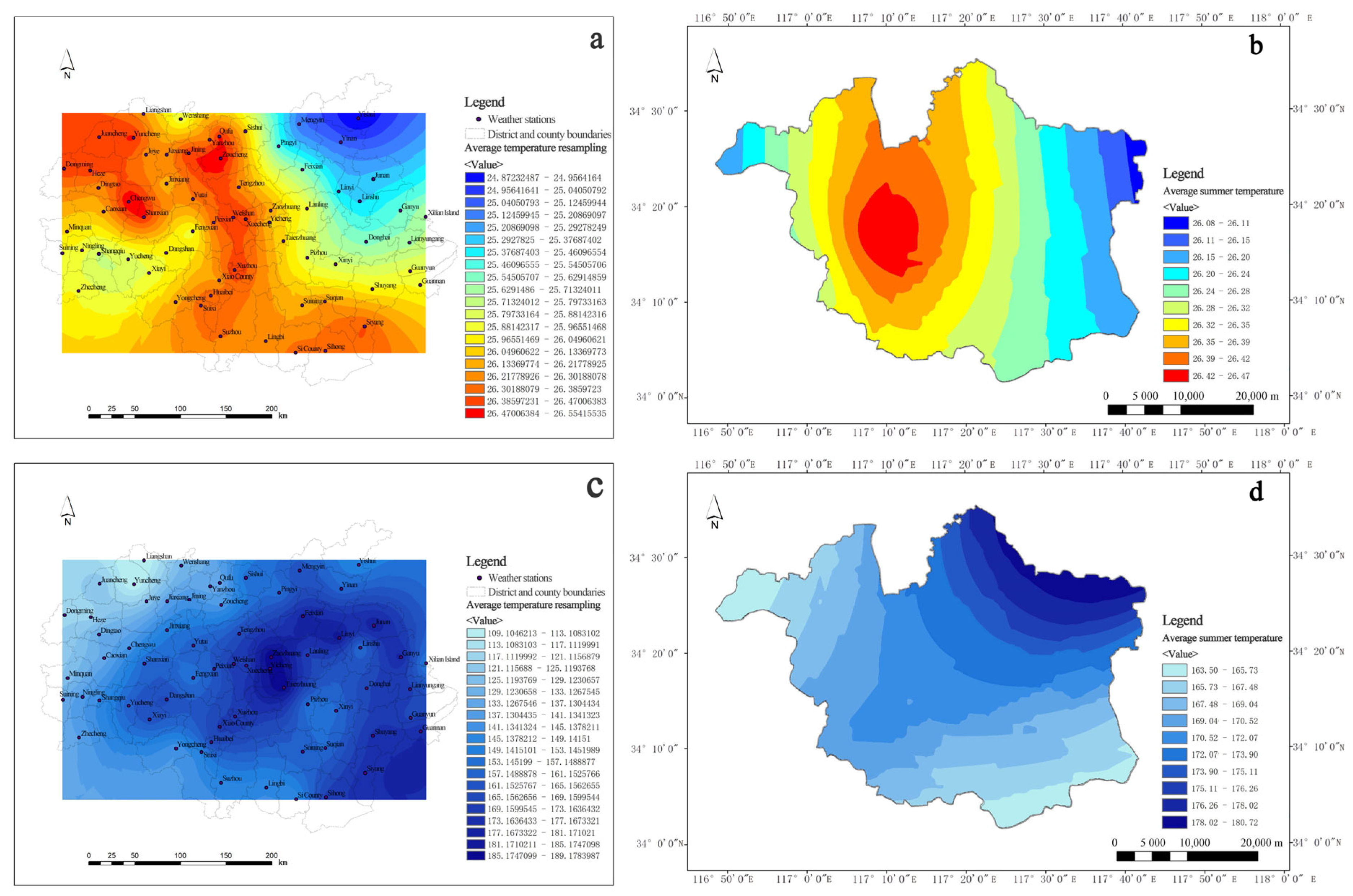
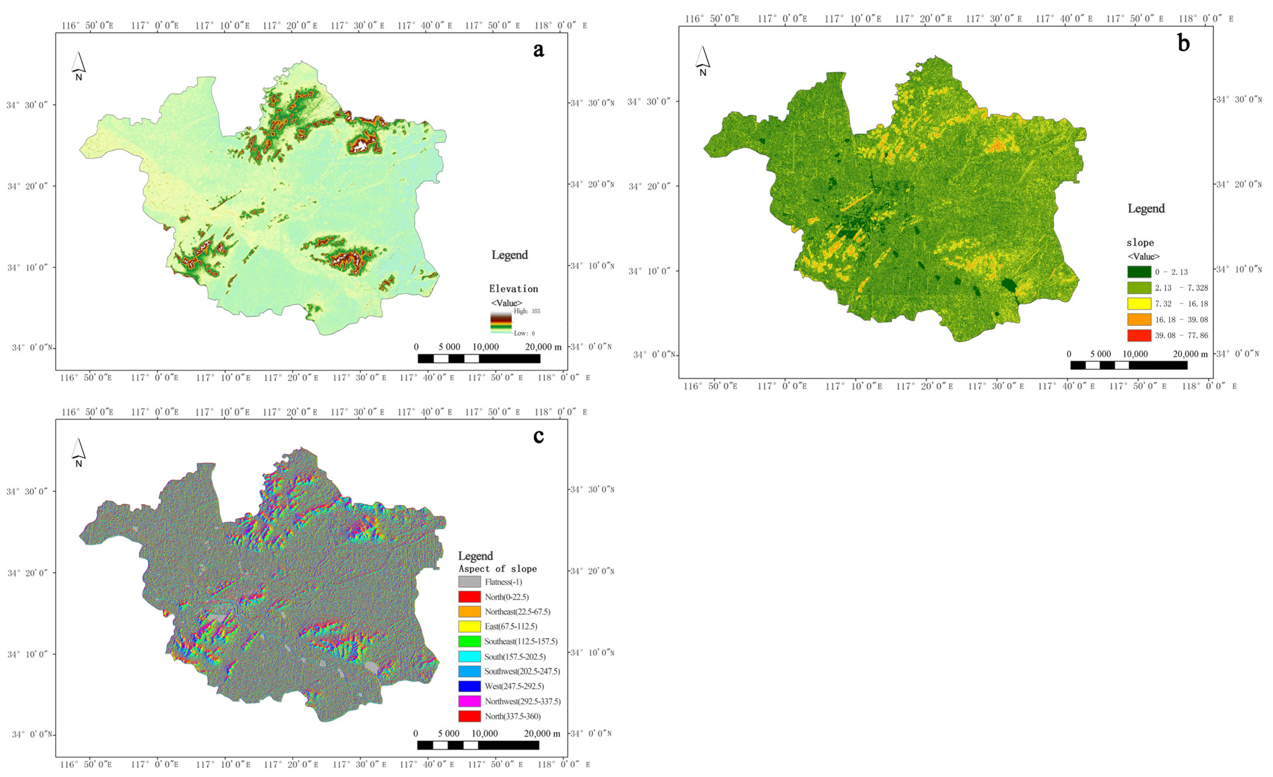
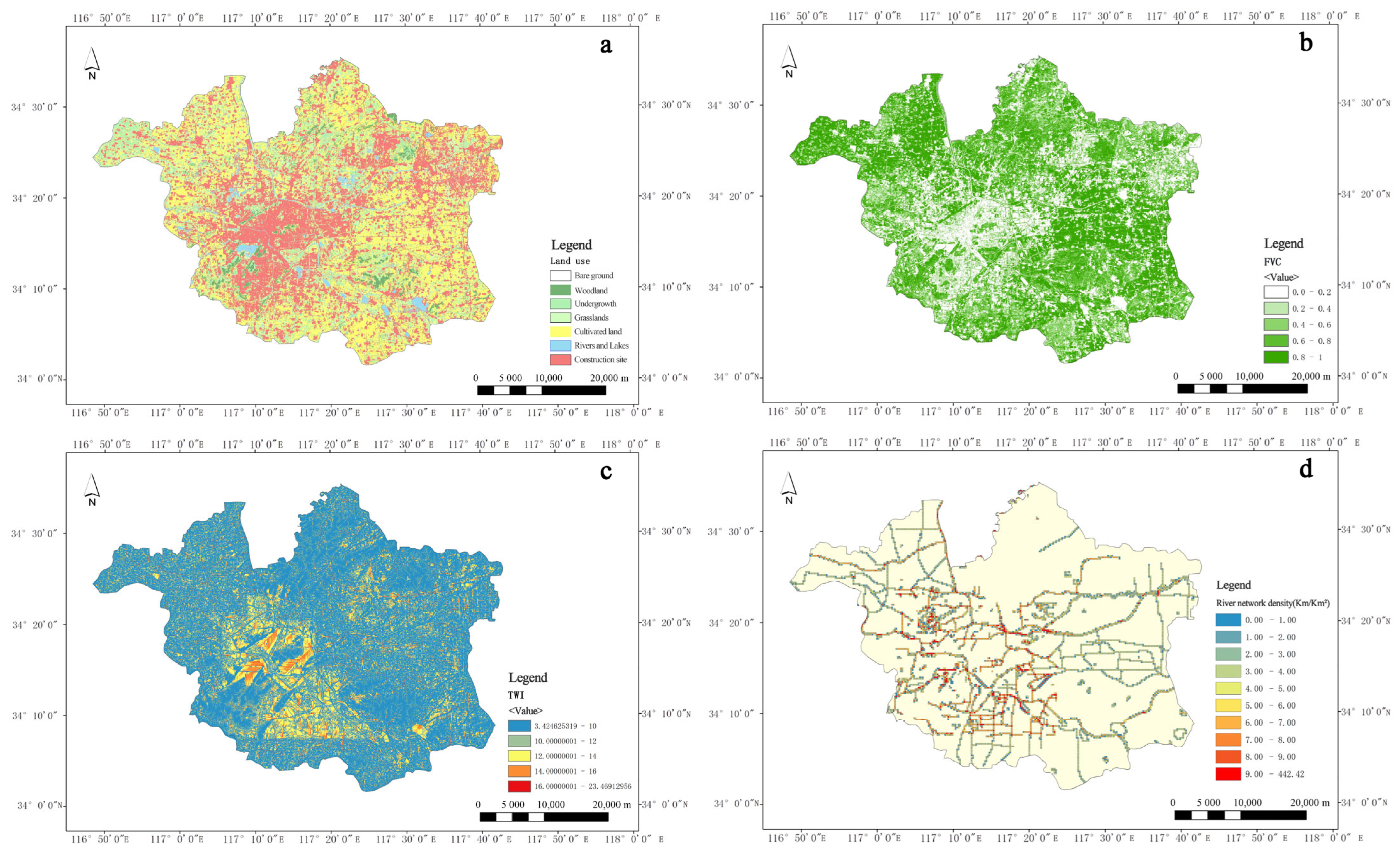
From the perspective of formation mechanism, climate, terrain, artificial surface, and natural surface work together to form water accumulation. The analysis results of the weights indicate that topography and climate play the most important influencing role in the formation of urban flooding. The intensity of heavy rain determines the occurrence of surface runoff. Topographic features affect the process of runoff convergence, which determines the probability of urban flooding formation. The characteristics of the natural surface and the artificial surface will have an impact on runoff and infiltration velocity. The above factors interact with each other and ultimately determine the formation of water accumulation.

This study provides a scientific basis for urban rain and waterlogging management in the Huang-Huai region, especially in the main city of Xuzhou. For the high-risk M5N5 and M5N4 areas (e.g., the old city and JiuLi Lake Wetland), it is recommended to prioritize the implementation of the “point-line-plane” integrated management strategy. Because high-risk areas are more vulnerable to rain and flooding and pose a greater threat to life safety. “Point-level” measures focus on the refined renovation of small and micro spaces, such as low-lying nodes, building ancillary facilities, and the storage and regulation facilities in old residential areas. Rain gardens, permeable pavements, green roofs, sunken tree pits, etc., can be renovated. The “line-level” measures focus on the improvement of the drainage system. Specifically, improvements can be made in rivers, waterways, and drainage corridors, such as repairing and widening rivers, upgrading rainwater networks, and laying drainage ditches along roadsides. At the “surface level”, measures should focus on ecological restoration of territorial space and zonal control of sponge cities. For instance, rivers and lakes should be connected through river networks and canals to enhance regulatory capabilities. In the zoning of sponge cities, the requirements for seepage and water storage indicators, as well as development restrictions should be strengthened. For medium-risk areas (e.g., M3N4, M4N3), community-level emergency response capacity should be strengthened, such as popularizing intelligent water level monitoring equipment in densely populated residential clusters and formulating graded evacuation plans. In addition, the “hidden risk areas” revealed by the research (such as the farmland runoff irrigation area in the south of the city) should prompt the planning department to break the status quo of urban-rural drainage system separation. Cross-regional deployment of stormwater resources is best achieved through integrated ditch-pipe network design. In the long run, the assessment of rainfall and waterlogging risk should be incorporated into the rigid constraints of territorial spatial planning, and the natural hydrological cycle should be gradually restored in conjunction with urban regeneration actions. Specific measures for these constraints can be to legalize the risk map or integrate the risk analysis process with the demarcation of the three zones and three lines. For instance, the area around Jiuli Lake Wetland can be designated as an ecological red line zone, prohibiting land reclamation from the lake. At the level of control detailed planning, indicators such as the total runoff control rate and the proportion of permeable area should be set. Thus, the urban area of Xuzhou ultimately achieves the collaborative goal of “reducing risks—optimizing space—enhancing resilience”. Countries such as Japan and the Netherlands have incorporated flood risks into their territorial spatial planning. China’s documents such as the “National Spatial Planning Law” and the “Guidelines for Sponge City Construction” explicitly state that flood risk assessment needs to be strengthened. Rigid constraints are a concrete manifestation of implementing the national strategy for disaster prevention and mitigation. At present, although China has also conducted evaluations of the carrying capacity of resources and the environment and the suitability of territorial space development. However, the rigid constraints on urban flooding in the evaluation content are too low. Raising the rigid defense standards can reduce a large amount of life and property losses every year. The old urban areas, which were developed earlier, are low-lying and prone to urban waterlogging. Promoting the prevention of urban flooding during urban renewal can achieve multiple benefits at once.

In the future, by integrating Internet of Things sensors, Geographic Information Systems (GIS), and real-time monitoring networks, machine learning models will be able to conduct dynamic modelling of urban water circulation systems, thereby optimizing rainwater runoff prediction, urban flooding risk assessment, and water resource scheduling strategies. For instance, the smart management and control platform for sponge cities established by Kunming collects multi-dimensional data through nearly 200 online monitoring stations. It uses machine learning algorithms to analyze rainwater volume, pollution load, and the operation status of pipe networks, achieving a transformation from “governance” to “intelligent management”, and significantly enhancing the efficiency of urban flood prevention and water resource utilization. This technological integration not only resolves the issue of data silos in traditional sponge city construction but also supports multi-scale system collaboration through simulation and optimization algorithms, such as balancing flood control and ecological demands at the basin scale, or precisely designing the storage and regulation capacity of rain gardens at the community scale.

5. Conclusions

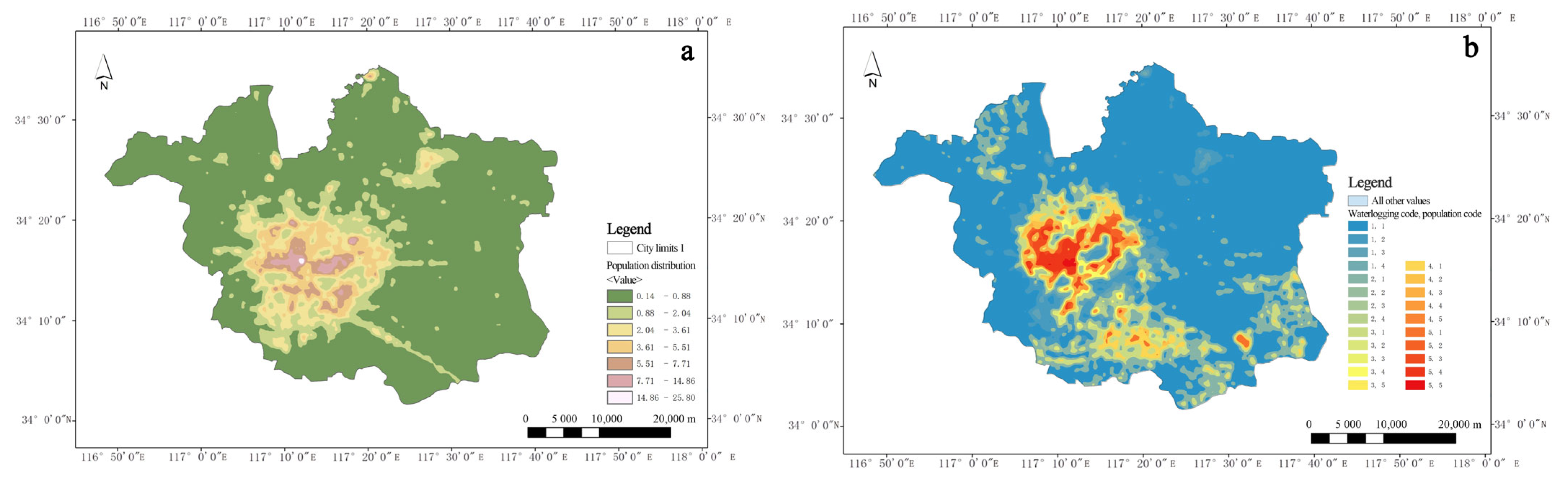
The study achieves a refined assessment of the coupled relationship between rainfall and flooding risk and population exposure in Xuzhou City by constructing a machine learning-based analytical model. The following conclusions were obtained: Firstly, from the perspective of technical approach, the CatBoost model has significant advantages in feature processing and nonlinear relationship capture, and its 81.67% accuracy rate verifies its applicability in complex geographic environments; Secondly, the fusion strategy of multi-source data (e.g., nighttime lighting data inversion of population distribution, dynamic correction of topographic factors) provides high-resolution data support for the study, which compensates for the spatial and temporal limitations of the traditional statistical methods; Thirdly, in addition to common waterlogging points in built-up areas, the study also identifies a large number of waterlogging points in peri-urban and rural areas; Fourthly, population densities of areas with high-risk of waterlogging are generally high, and high-risk of waterlogging is shown in the old urban area, the northwestern section and the southern part of the city, all of which are characterized by high-risk, high exposure. However, there are also shortcomings in this paper. Firstly, the insufficient spatio-temporal resolution of the data makes it difficult to capture the local heavy rainfall and sudden changes in surface confluence caused by urban micro-topography, resulting in inaccurate predictions of urban waterlogging hotspots. Secondly, the existing models rely on static infrastructure parameters (such as drainage pipe networks) and do not integrate real-time sensor data (such as manhole cover water levels and pump station status), which weakens the response capability to emergencies such as pipe network blockages or equipment failures. Furthermore, the heterogeneity of multi-source data (such as the format differences of meteorological satellites and social media warnings) limits the dynamic fusion ability of the model, making it difficult to achieve minute-level coupling of “meteorology—hydrology—society” data. In the future, it is necessary to integrate high-resolution radar precipitation forecasting, IoT sensor networks, and reinforcement learning algorithms to construct a digital twin system that ADAPTS to the evolution of urban rain and flood.

References

1. Zhai, G. Urban resilience response to rain and flood damage from the planning perspective in the context of climate change: Key concepts, basic ideas and general framework. J. Urban Plan. 2024, 1, 29–37. [Google Scholar] [CrossRef]
2. Lenton, T.M.; Rockström, J.; Gaffney, O.; Rahmstorf, S.; Richardson, K.; Steffen, W.; Schellnhuber, H.J. Climate tipping points—Too risky to bet against. Nature 2019, 575, 592–595. [Google Scholar] [CrossRef]
3. Wu, Z.; Yan, J.; Xu, H.; Chen, Z.; Wei, R.; Wu, T.; Geng, X. Ten key topics in the development of urban and rural planning (2024–2025). J. Urban Plan. 2004, 6, 8–11. [Google Scholar] [CrossRef]
4. Yan, Y.; Wang, H.; Li, G.; Xia, J.; Ge, F.; Zeng, Q.; Ren, X.; Tan, L. Projection of Future Extreme Precipitation in China Based on the CMIP6 from a Machine Learning Perspective. Remote Sens. 2022, 14, 4033. [Google Scholar] [CrossRef]
5. Yu, K.; Li, H.; Li, D.; Qiao, Q.; Xi, X. Ecological security pattern at territorial scale. Acta Ecol. Sin. 2009, 29, 5163–5175. [Google Scholar]
6. Zhang, M.; Tan, S.; Zhang, C.; Chen, E. Machine learning in modelling the urban thermal field variance index and assessing the impacts of urban land expansion on seasonal thermal environment. Sustain. Cities Soc. 2024, 106, 105345. [Google Scholar] [CrossRef]
7. Zhao, X.; Li, H.; Cai, Q.; Pan, Y.; Qi, Y. Managing extreme rainfall and flooding events: A case study of the 20 July 2021 Zhengzhou flood in China. Climate 2023, 11, 228. [Google Scholar] [CrossRef]
8. Arjenaki, M.O.; Sanayei, H.R.Z.; Heidarzadeh, H.; Mahabadi, N.A. Modeling and investigating the effect of the LID methods on collection network of urban runoff using the SWMM model (case study: Shahrekord City). Model. Earth Syst. Environ. 2020, 7, 1–16. [Google Scholar] [CrossRef]
9. Ogras, S.; Onen, F. Flood Analysis with HEC-RAS: A Case Study of Tigris River. Adv. Civ. Eng. 2020, 2020, 6131982. [Google Scholar] [CrossRef]
10. Tan, M.L.; Gassman, P.W.; Yang, X.; Haywood, J. A review of SWAT applications, performance and future needs for simulation of hydro-climatic extremes. Adv. Water Resour. 2020, 143, 103662. [Google Scholar] [CrossRef]
11. Dai, X.; Huang, H.; Ji, X.; Wang, W. Based on machine learning urban rainstorm waterlogging time fast prediction model. J. Tsinghua Univ. (Nat. Sci. Ed.) 2023, 6, 865–873. [Google Scholar] [CrossRef]
12. Tang, X.; Tian, J.; Huang, X.; Shu, Y.; Liu, Z.; Long, S.; Xue, W.; Liu, L.; Lin, X.; Liu, W. A novel machine learning-based framework to extract the urban flood susceptible regions. Int. J. Appl. Earth Obs. Geoinf. 2024, 132, 104050. [Google Scholar] [CrossRef]
13. Seckin, N.; Cobaner, M.; Yurtal, R.; Haktanir, T. Comparison of artificial neural network methods with L-moments for estimating flood flow at ungauged sites: The case of east Mediterranean river basin, turkey. Water Resour. Manag. 2013, 27, 2103–2124. [Google Scholar] [CrossRef]
14. Jones, A.; Kuehnert, J.; Fraccaro, P.; Meuriot, O.; Ishikawa, T.; Edwards, B.; Stoyanov, N.; Remy, S.L.; Weldemariam, K.; Assefa, S. AI for climate impacts: Applications in flood risk. npj Clim. Atmos. Sci. 2023, 6, 63. [Google Scholar] [CrossRef]
15. Lin, K.; OuYang, J.; Ma, X.; Xiao, M.; Feng, X. Prediction model of urban waterlogging water depth based on deep learning. Water Resour. Prot. 2019, 41, 56–63. [Google Scholar]
16. Kalteh, A.M. Monthly river flow forecasting using artificial neural network and support vector regression models coupled with wavelet transform. Comput. Geosci. 2013, 54, 1–8. [Google Scholar] [CrossRef]
17. Wang, W.-C.; Chau, K.-W.; Cheng, C.-T.; Qiu, L. A comparison of performance of several artificial intelligence methods for forecasting monthly discharge time series. J. Hydrol. 2009, 374, 294–306. [Google Scholar] [CrossRef]
18. Zeng, P. Machine Learning Technology in the Application of City Flood Rapid Prediction Research. Master’s Thesis, China Water Resources and Hydropower Research Institute, Beijing, China, 2020. [Google Scholar]
19. Yan, J.; Jin, J.; Chen, F.; Yu, G.; Yin, H.; Wang, W. Urban flash flood forecast using support vector machine and numerical simulation. J. Hydroinform. 2017, 20, 221–231. [Google Scholar] [CrossRef]
20. Wang, H.; Zhao, Y.; Zhou, Y.; Wang, H. Prediction of urban water accumulation points and water accumulation process based on machine learning. Earth Sci. Inform. 2021, 14, 2317–2328. [Google Scholar] [CrossRef]
21. Li, H.; Wu, J.; Wang, Q.; Yang, C.; Pan, S. Based on machine learning method of rainstorm waterlogging disaster prediction model of Shanghai research. J. Nat. Disasters 2021, 30, 191–200. [Google Scholar] [CrossRef]
22. Berkhahn, S.; Fuchs, L.; Neuweiler, I. An ensemble neural network model for real-time prediction of urban floods. J. Hydrol. 2019, 575, 743–754. [Google Scholar] [CrossRef]
23. Tang, X.; Huang, X.; Tian, J.; Pan, S.; Ding, X.; Zhou, Q.; Sun, C. A novel framework for the spatiotemporal assessment of urban flood vulnerability. Sustain. Cities Soc. 2024, 109, 105523. [Google Scholar] [CrossRef]
24. Mabdeh, A.N.; Ajin, R.S.; Razavi-Termeh, S.V.; Ahmadlou, M.; Al-Fugara, A. Enhancing the Performance of Machine Learning and Deep Learning-Based Flood Susceptibility Models by Integrating Grey Wolf Optimizer (GWO) Algorithm. Remote Sens. 2024, 16, 2595. [Google Scholar] [CrossRef]
25. Lyu, H.-M.; Yin, Z.-Y. Flood susceptibility prediction using tree-based machine learning models in the GBA. Sustain. Cities Soc. 2023, 97, 104744. [Google Scholar] [CrossRef]
26. Sutton, P. Modeling population density with night-time satellite imagery and GIS. Comput. Environ. Urban Syst. 1997, 21, 227–244. [Google Scholar] [CrossRef]
27. Gong, Y.-X.; Chu, Y.; Cheng, S.-S. Based on night light data and spatial regression models of population grid handling method research. J. Jinling Inst. Technol. 2024, 40, 1–12. [Google Scholar] [CrossRef]
28. Yang, J.; Duan, C.; Wang, H.; Chen, B. Spatial supply-demand balance of green space in the context of urban waterlogging hazards and population agglomeration. Resour. Conserv. Recycl. 2022, 188, 106662. [Google Scholar] [CrossRef]
29. Elvidge, C.D.; Cinzano, P.; Pettit, D.R.; Arvesen, J.; Sutton, P.; Small, C.; Nemani, R.; Longcore, T.; Rich, C.; Safran, J.; et al. The Nightsat mission concept. Int. J. Remote Sens. 2007, 28, 2645–2670. [Google Scholar] [CrossRef]
30. Chen, Z.; Yu, B.; Hu, Y.; Huang, C.; Shi, K.; Wu, J. Estimating house vacancy rate in metropolitan areas using NPP-VIIRS nighttime light composite data. IEEE J. Sel. Top. Appl. Earth Obs. Remote Sens. 2015, 8, 2188–2197. [Google Scholar] [CrossRef]
31. Chen, H.; Xu, Z.; Liu, Y.; Huang, Y.; Yang, F. Urban flood risk assessment based on dynamic population distribution and fuzzy comprehensive evaluation. Int. J. Environ. Res. Public Health 2022, 19, 16406. [Google Scholar] [CrossRef]
32. Deng, H.; Zhang, K.; Wang, F.; Dang, A. Compact or disperse? Evolution patterns and coupling of urban land expansion and population distribution evolution of major cities in China, 1998–2018. Habitat Int. 2021, 108, 102324. [Google Scholar] [CrossRef]
33. Elvidge, C.D.; Sutton, P.C.; Ghosh, T.; Tuttle, B.T.; Baugh, K.E.; Bhaduri, B.; Bright, E. A global poverty map derived from satellite data. Comput. Geosci. 2009, 35, 1652–1660. [Google Scholar] [CrossRef]
34. Chen, T.; Zhu, Q.; Chang, J. Landscape perspective of Xuzhou urban spatial pattern study. J. Cent. China Build. 2020, 38, 71–75. [Google Scholar] [CrossRef]
35. Dai, P.; Shen, Z. Water environment changes and the rise and fall of Xuzhou city research. J. Hum. Geogr. 2013, 28, 55–61. [Google Scholar] [CrossRef]
36. Yu, W.; Li, J.; Yu, R. Seasonal variation of precipitation persistence in China. Meteorology 2012, 38, 392–401. [Google Scholar]
37. Li, H.-h.; Wu, J.-d. Rainstorm characteristics and its relationship with waterlogging disaster in shanghai during 2007–2016. J. Nat. Resour. 2018, 33, 2136–2148. [Google Scholar] [CrossRef]
38. Liu, W.; Zhang, X.; Feng, Q.; Yu, T.; Engel, B.A. Analyzing the impacts of topographic factors and land cover characteristics on waterlogging events in urban functional zones. Sci. Total. Environ. 2023, 904, 166669. [Google Scholar] [CrossRef]
39. Huang, J.; Li, J.; Huang, Z. Identification of Waterlogging-Prone Areas in Nanning from the Perspective of Urban Expansion. Sustainability 2023, 15, 15095. [Google Scholar] [CrossRef]
40. Zhang, M.; Xu, M.; Wang, Z.; Lai, C. Assessment of the vulnerability of road networks to urban waterlogging based on a coupled hydrodynamic model. J. Hydrol. 2021, 603, 127105. [Google Scholar] [CrossRef]
41. Jiang, Y.; Li, J.; Li, Y.; Gao, J.; Xia, J. Influence of rainfall pattern and infiltration capacity on the spatial and temporal inundation characteristics of urban waterlogging. Environ. Sci. Pollut. Res. 2024, 31, 12387–12405. [Google Scholar] [CrossRef]
42. Wang, L.; Huang, Y.; Wang, K.; Jian, Z. Risk zone assessment of rainstorm induced waterlogging associated outage of distribution system with con-sideration of micro topography. J. Electr. Power Sci. Technol. 2024, 39, 84–92. [Google Scholar] [CrossRef]
43. Dwivedi, R.S.; Sreenivas, K. The vegetation and waterlogging dynamics as derived from spaceborne multispectral and multitemporal data. Int. J. Remote Sens. 2002, 23, 2729–2740. [Google Scholar] [CrossRef]
44. Liu, S.; Lin, M.; Li, C. Analysis of the effects of the river network structure and urbanization on waterlogging in high-density urban areas—A case study of the Pudong New Area in Shanghai. Int. J. Environ. Res. Public Health 2019, 16, 3306. [Google Scholar] [CrossRef]
45. Hassan, A.; Belal, A.; Hassan, M.; Farag, F.; Mohamed, E. Potential of thermal remote sensing techniques in monitoring waterlogged area based on surface soil moisture retrieval. J. Afr. Earth Sci. 2019, 155, 64–74. [Google Scholar] [CrossRef]
46. Liu, Y.; Chen, B.; Duan, C.; Wang, H. Economic loss of urban waterlogging based on an integrated drainage model and network environ analyses. Resour. Conserv. Recycl. 2023, 192, 106923. [Google Scholar] [CrossRef]
47. Ma, F.; Ao, Y.; Wang, X.; He, H.; Liu, Q.; Yang, D.; Gou, H. Assessing and enhancing urban road network resilience under rainstorm waterlogging disasters. Transp. Res. Part D Transp. Environ. 2023, 123, 103928. [Google Scholar] [CrossRef]
48. Wang, J.; Lin, C.; Liang, F.; Ji, J.; Tang, S.; Liu, Y. Landslide susceptibility analysis and adaptive evaluation based on different machine learning models. Sci. Technol. Eng. 2019, 25, 513–520. [Google Scholar] [CrossRef]
Figure 1. Location map and waterlogging points distribution.
Land 14 00939 g001
Figure 2. Meteorological factor analysis chart. (a) Temperature in the Huanghuai region; (b) The temperature in Xuzhou urban area; (c) Rainfall in the Huanghuai region; (d) Rainfall in Xuzhou urban area; (e) Wind speed in the Huanghuai region; (f) Wind speed in Xuzhou urban area.
Land 14 00939 g002aLand 14 00939 g002b
Figure 3. Results of terrain analysis chart. (a) Elevation; (b) Slope; (c) Aspect of slope.
Land 14 00939 g003
Figure 4. Natural surface factor analysis chart. (a) land use; (b) Degree of vegetation coverage; (c) topographic wetness index; (d) River network density.
Land 14 00939 g004
Figure 5. Artificial surface factor analysis chart. (a) Density of rainwater pipe network; (b) Road network density; (c) Railroad network density.
Land 14 00939 g005
Figure 6. Technology roadmap.
Land 14 00939 g006
Figure 7. Functional relationship diagram.
Land 14 00939 g007
Figure 8. Confusion Matrix Result Chart. (In classification tasks, the darker the color of the main diagonal (correct prediction), the better the prediction effect of the model).
Land 14 00939 g008
Figure 9. Parametric radar charts. (a) Machine learning parameter comparison chart; (b) Machine learning parameters of non-water waterlogging points; (c) Machine learning parameters of water waterlogging points.
Land 14 00939 g009
Figure 10. Waterlogging point distribution map and nuclear density analysis map. (a) Waterlogging points distribution map; (b) Nuclear density analysis map of waterlogging points.
Land 14 00939 g010
Figure 11. Population density map and waterlogged coupling risk map. (a) Population density map; (b) Waterlogged coupling risk map.
Land 14 00939 g011