Unmanned Aerial Vehicles Applicability to Mapping Soil Properties Under Homogeneous Steppe Vegetation

Abstract

Unmanned aerial vehicles (UAVs) are rapidly becoming a popular tool for digital soil mapping at a large-scale. However, their applicability in areas with homogeneous vegetation (i.e., not bare soil) has not been fully investigated. In this study, we aimed to predict soil organic carbon, soil texture at several depths, as well as the thickness of the AB soil horizon and penetration resistance using a machine learning algorithm in combination with UAV images. We used an area in the Eurasian steppe zone (Republic of Bashkortostan, Russia) covered with the Stipa vegetation type as a test plot, and collected 192 soil samples from it. We estimated the models using a cross-validation approach and spatial prediction uncertainties. To improve the prediction performance, we also tested the inclusion of oblique geographic coordinates (OGCs) as covariates that reflect spatial position. The following results were achieved: (i) the predictive models demonstrated poor performance using only UAV images as predictors; (ii) the incorporation of OGCs slightly improved the predictions, whereas their uncertainties remained high. We conclude that the inability to accurately predict soil properties using these predictor variables (UAV and OGC) is likely due to the limited access to soil spectral signatures and the high variability of soil properties within what appears to be a homogeneous site, particularly in relation to soil-forming factors. Our results demonstrated the limitations of UAVs’ application for modeling soil properties on a site with homogeneous vegetation, whereas including spatial autocorrelation information can benefit and should be not ignored in further studies.

1. Introduction

Spatial soil information is necessary for a variety of applications, including agriculture, land use planning, and climate change mitigation. Conventional soil mapping relies on field sampling and laboratory analyses, making it a time-consuming and expensive process [1,2]. In recent decades, digital soil mapping (DSM) has emerged as a promising tool to overcome these challenges and improve the accuracy of soil maps and the prediction of soil properties [3]. DSM utilizes environmental predictors (covariates) and statistical models to produce spatial soil products from various data sources. Remote sensing data are a covariate type that represent organisms in the SCORPAN model [3] and are one of the crucial predictors in DSM, providing valuable information about vegetation cover and land use types [4]. However, freely available remote sensing data often suffer from limitations in spatial resolution, making it difficult to capture fine-scale soil variations. This constraint necessitates the use of high-resolution data, which may be expensive, posing a challenge for widespread application of them in soil mapping.

Unmanned aerial vehicles (UAVs) have revolutionized DSM and their features. These versatile platforms offer advantages for soil monitoring and mapping. Their ability to fly at low altitudes and capture high-resolution images allows for the identification of subtle variations in soil properties, such as color, texture, and vegetation cover [5,6,7]. This level of detail is crucial for accurate soil mapping at a field scale [8], as well as in areas with complex landscapes and diverse soil types. UAV deployment is quick and efficient, making them ideal for rapid assessments and monitoring of soil conditions over time. Recently, UAVs have been used to map a range of soil properties and processes, such as soil organic carbon (SOC) [9,10], nitrogen [11], texture [12], moisture [13], and erosion [14,15].

For croplands, the success of the predictive mapping of properties—mainly SOC or texture—using remote sensing data often hinges on the relationship between spectral reflectance and bare soil surface conditions, such as color or moisture [16]. For instance, darker soil colors typically indicate higher organic carbon content compared to paler soils [17]. When modeling soil properties among heterogeneous landscapes, land use patterns are a key predictor because of differences in carbon decomposition. A typical case is where pristine soils are generally characterized by increased carbon content compared to similar arable soils [18,19]. Therefore, while remote sensing can be valuable for mapping soil properties in bare conditions or heterogeneous landscapes, its effectiveness may be limited in areas with homogeneous vegetation, like forests or steppes.

DSM relies heavily on covariates to accurately model soil properties. Unlike geostatistical methods, which account for the spatial autocorrelation of soil properties (i.e., the tendency of nearby locations to have similar soil properties), machine learning algorithms typically disregard it because they are basically non-spatial [20]. Thus, it is a disadvantage, because soil parameters are typically characterized by a spatial trend [21]. As demonstrated by several studies, incorporating geographic position as a covariate can enhance predictions [22,23,24,25], particularly in areas with gradual soil gradients or where spatial autocorrelation is present.

In this study, we aimed to test the ability to predict a number of basic soil properties at several depths using UAV data as covariates. We hypothesize that the uniform vegetation cover in the study area may pose challenges for modeling soil properties compared to modeling on croplands (i.e., bare soil). To overcome this challenge, we also tested the incorporation covariates that take spatial location into account using state-of-the-art machine learning techniques. Hence, the primary purpose of this research is to evaluate the feasibility of UAV-based DSM in densely vegetated areas and develop methodological adaptations that enhance soil property predictions when traditional remote sensing approaches are limited by vegetation interference.

2. Materials and Methods

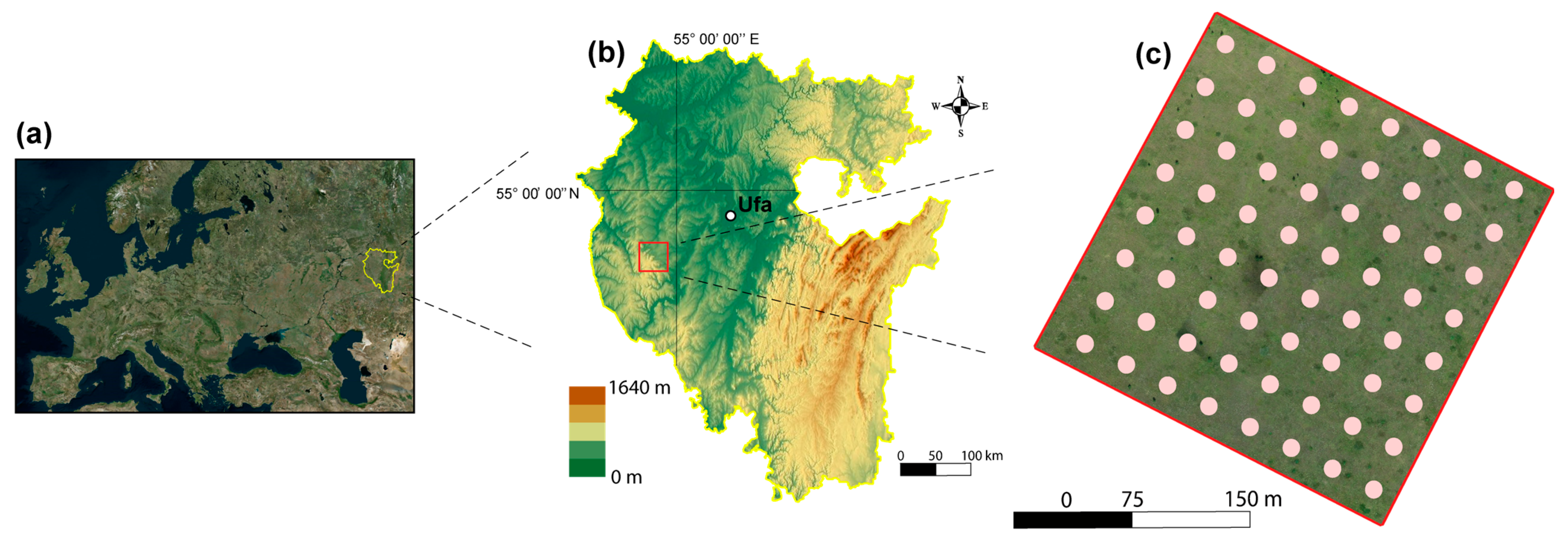
2.1. Study Area

The research was conducted on the test plot (250 × 250 m) within the carbon polygon “Kovylnaya Steppe” site, located in the meadow steppe 3.5 km south of the village of Kuryatmasovo in the Davlekanovsky District of the Republic of Bashkortostan (Russia) (Figure 1). According to international botanical and geographical zoning, the study area belongs to the Eurasian steppe, and according to local classification, it belongs to the steppe zone of the Cis-Urals. The test plot is located on a leveled ridge top, is characterized by a slight slope to the northwest; the altitude ranges from 413–418 m a.s.l. The studied territory was previously used as arable land (according to space images, for at least 30 years), and from the early 2000s to the present time, it has been abandoned. However, haymaking occurs on the study site occasionally.

The climate of the study area is continental, with insufficient moisture (Dfb, according to the Köppen–Geiger climate classification [26]). The average annual air temperature is +3.3 °C; the average January temperature is –14.2 °C; July is +20 °C; the average depth of soil freezing by the end of winter is up to 90–130 cm. The average annual precipitation is 450 mm, the frost-free period lasts 125 days, and the vegetation period lasts 170 days [27].

The projective cover of grass stand at the time of survey (summer 2022) was 70–85%, and the average height 40 cm. The vegetation was dominated by turf grasses (European feather grass—Stipa pennata; hairy feather grass—Stipa capillata; false sheep fescue—Festuca pseudovina) and the rhizomatous-loose-bunch grass narrow-leaved meadow-grass (Poa angustifolia). Among the herbs with a relatively large abundance are the Asian agrimony (Agrimonia asiatica), the burnet-saxifrage (Pimpinella saxifraga), the zigzag clover (Trifolium medium), the tuberous pea (Lathyrus tuberosus), and the lesser meadow-rue (Thalictrum minus), etc. The floristic composition is close to the natural rich-forb meadow steppes of the studied region: the flora is dominated in approximately equal proportions by meadow-steppe (36.6% of the total flora of vascular plants) and meadow (33.7%) species; steppe species make up 12.8%; 12 weed species (11.9%) were identified, which are mainly segetal weeds of row crops (leafy spurge—Euphorbia virgata; field bindweed—Convolvulus arvensis; bitter wormwood—Artemisia absinthium, etc.) and, apparently, have survived since the time the site was used as arable land. All plant species were distributed on the studied plot uniformly (Figure 2a).

2.2. Soil Characteristic, Sampling, and Laboratory Analysis

For soil type determination, 2 profile pits (3 m in length, 1 m in width, and 0.5 m in depth; Figure 2c) were excavated (to the parent material) near the opposite corners of the test plot. After morphological property description, the soil cover of the study area was determined as Calcic Chernozem [28].

Soil samples were taken within the test plot at 64 points (from a depth of 0–30, 30–60 and 60–90 cm; total of 192 samples) using a JMC hand-driven core sampler (Clements Associates Inc., Newton, MA, USA; inner diameter: 4.5 cm) via an 8×8 grid scheme. During soil sampling/drilling, the thickness of the humus-accumulative (AB) horizon also was measured (Figure 2c). The soil samples (~50 g) were collected in a plastic bag and then delivered to a laboratory. The stones and tree/plant roots were removed from the samples, then samples were air-dried to constant weight, ground in a mortar, and sieved through a 2 mm sieve for further analysis. The SOC in the soil samples was determined by the wet-combustion method according to Tyurin [29] (direct analog of Walkley–Black method [30]) using a Specord M40 spectrophotometer (VEB Carl Zeiss, Jena, Germany). The particle size distribution was measured by a Laska-TD laser diffraction analyser (Biomedical Systems, Russia) with the following size gradation: clay (0–2 µ), silt (2–50 µ), and sand (50–500 µ). Soil penetration was measured from the soil surface to a depth of 45 cm with 2.5 cm intervals by using the soil compaction meter FieldScout SC 900 (Spectrum technologies, Aurora, CO, USA), equipped with a metal rod with a cone (size 1/2 inch).

2.3. Unmanned Aerial Vehicle Imaging

The UAV data were collected in the summer of 2022 on a dry, sunny, and cloudless day. A DJI Phantom 4 RTK drone was employed for RGB imagery acquisition (Figure 2d). The drone flew at an altitude of 100 m, following a pre-planned flight path, to capture aerial images of the study area using a grid pattern. Images were acquired with a standard 60% overlap to ensure high-quality orthomosaic creation. Image alignment, stitching, and digital surface model generation were performed using standard procedures in Agisoft Metashape Professional version 1.7.

2.4. Environmental Variables

The set of 13 covariates derived from the UAV data, including spectral indices and terrain data, were calculated (Table 1). Using the RGB bands from the UAV, we calculated the spectral indices. Also, a digital surface model and then a slope map were calculated from the UAV images. Although the acquired images have ultra-high spatial resolution (2.74 cm/px), we reduced this value to 1 m/px using the aggregate function in R statistics software (4.4.2) to eliminate artifacts and reduce computational costs.

Explicitly spatial covariates included oblique geographic coordinates (OGCs) at six angles, as earlier demonstrated by Møller et al. [24]. In total, six OGCs (π = 0, 0.17, 0.33, 0.5, 0.67, and 0.83) were calculated, as shown in Figure 3. The OGC at an angle of θ can be calculated as in Equation (1) below:

$$OGC=\sqrt{X^2+Y^2}\times cos\left(\theta -{tan}^{-1}\left({\displaystyle \frac{Y}{X}}\right)\right)$$

(1)

where X and Y are the latitude and longitude, respectively; θ is the angle of the titled axis relative to the x axis.

Pre-processing and harmonization of the covariates involved several steps: (1) conversion to the same coordinate system (EPSG:3395); and (2) aggregating of covariates into a 1 m resolution, using a bilinear interpolation method. These steps were performed with “terra” package [31] in R. We tested two scenarios for digital mapping of soil properties, among which the first scenario included only a UAV dataset as predictors, while the second scenario included UAV and positional covariates (OGCs) together.

Table 1. Environmental variables.

Covariate Type	Name	Abbreviation	Details	Reference
Organisms	Red	R	RGB red band	Our source
Organisms	Green	G	RGB green band	Our source
Organisms	Blue	B	RGB blue band	Our source
Organisms	Normalized red	Rn	R/(R + G + B)	Kawashima et al. [32]
Organisms	Normalized green	Gn	G/(R + G + B)	Kawashima et al. [32]
Organisms	Normalized blue	Rn	B/(R + G + B)	Kawashima et al. [32]
Organisms	Brightness index	BI	sqrt [(R2 + G2 + B2)/3]	Levin et al. [33]
Organisms	Coloration index	CI	(R − G)/(R + G)	Levin et al. [33]
Organisms	Hue index	HI	(2 × R − G − B)/(G − B)	Levin et al. [33]
Organisms	Green red difference index	GRDI	(G − R)/(G + R)	Tucker [34]
Organisms	Saturation index	SI	(R − B)/(R+ B)	Levin et al. [33]
Relief	Digital surface model	dsm	Elevation above sea level	Our source
Relief	Slope	Slope	Slopes in degrees	Our source
Position	Oblique geographic coordinates	OGC	Six covariates (π = 0, 0.17, 0.33, 0.5, 0.67, and 0.83)	Møller et al. [24]

Table 1. Environmental variables.

Covariate Type	Name	Abbreviation	Details	Reference
Organisms	Red	R	RGB red band	Our source
Organisms	Green	G	RGB green band	Our source
Organisms	Blue	B	RGB blue band	Our source
Organisms	Normalized red	Rn	R/(R + G + B)	Kawashima et al. [32]
Organisms	Normalized green	Gn	G/(R + G + B)	Kawashima et al. [32]
Organisms	Normalized blue	Rn	B/(R + G + B)	Kawashima et al. [32]
Organisms	Brightness index	BI	sqrt [(R2 + G2 + B2)/3]	Levin et al. [33]
Organisms	Coloration index	CI	(R − G)/(R + G)	Levin et al. [33]
Organisms	Hue index	HI	(2 × R − G − B)/(G − B)	Levin et al. [33]
Organisms	Green red difference index	GRDI	(G − R)/(G + R)	Tucker [34]
Organisms	Saturation index	SI	(R − B)/(R+ B)	Levin et al. [33]
Relief	Digital surface model	dsm	Elevation above sea level	Our source
Relief	Slope	Slope	Slopes in degrees	Our source
Position	Oblique geographic coordinates	OGC	Six covariates (π = 0, 0.17, 0.33, 0.5, 0.67, and 0.83)	Møller et al. [24]

2.5. Digital Mapping Procedure

The random forest (RF) algorithm was used for digital mapping of soil properties. This machine learning technique is an ensemble learning method that combines multiple decision trees to improve predictive accuracy [35]. Each decision tree in the forest is constructed using a randomly selected subset of input variables and training samples. RF produces predictions by aggregating the results from individual trees, resulting in robust and reliable predictions.

We employed the recursive feature elimination (RFE) algorithm to select the most significant auxiliary variables in predicting soil parameters [36]. RFE is a feature selection method that iteratively removes features (covariates) from a dataset based on their importance. RFE helps to reduce model complexity, improve generalization, and enhance interpretability by identifying the most influential predictors.

The RF model for each target variable at a corresponding depth was tuned using several hyperparameters (mtry, splitrule, and nodesize) to achieve the highest accuracy, whereas the ntree parameter was set to the default value of 500. The RF model with the lowest root mean squared error (RMSE) after a 5-fold cross-validation procedure was selected for a further digital mapping process.

We assessed the importance of the covariates in each RF model using a permutation method. This involved randomly shuffling the values of each variable and observing the impact on model accuracy, allowing us to rank variables based on their influence on predictions. Digital mapping process, as well as model tuning, variable importance assessment, and cross-validation were performed with the “caret” package [37] in R.

2.6. Uncertainty Assessment and Model Evaluation

We accompanied each spatial prediction of the target variable with an assessment of uncertainty propagation using the Quantile Regression Forest [38] approach. QRF is an extension of RF that allows one to estimate conditional quantiles for target variables. The spatial uncertainty of the predicted properties was generated by the upper (95% quantile) and lower (5% quantile) percentile predictions, showing the width of the 90% prediction interval. A 90% prediction interval is a range of values that are likely to contain a future observation of a variable, with a 90% level of confidence.

For the assessment of the accuracy of predictive models, a 5-fold cross-validation procedure with fifty repetitions was applied. Model performance was based on two validation indices: RMSE and coefficient of determination (R²). In the reported results, RMSE is considered optimal when it approaches 0, whereas R² is considered ideal when it is equal to 1. The RMSE and R² error metrics are calculated as follows:

$$RMSE=\sqrt{{\displaystyle \frac{{\sum }_{i=0}^n{\left(O_i{-P}_i\right)}^2}{n}}}$$

(2)

$$R^2={\left({\displaystyle \frac{{\sum }_{i=0}^n\left(O_i-O_{avg}\right)\times \left(P_i-P_{avg}\right)}{\sqrt{{\sum }_{i=0}^n{\left(O_i{-O}_{avg}\right)}^2}\times {\left(P_i-P_{avg}\right)}^2}}\right)}^2$$

(3)

where O_i and P_i are the observed and predicted values of the soil property at a corresponding depth, O_avg and P_avg are the average values, and n is the number of samples.

3. Results

3.1. Descriptive Statistics of Soil Properties

For each variable,

Table 2. Descriptive statistics of soil properties at various depths.

Soil Property	Depth, cm	Min	Max	Mean	Median	Kurtosis	SD	CV, %
SOC, %	0–30	3.77	8.58	6.6	6.72	0.24	0.94	14.27
	30–60	0.46	6.96	2.67	2.63	0.49	1.34	50.25
	60–90	0.06	2.78	1.03	1	−0.26	0.67	65.58
Clay, %	0–30	0.91	38.62	7.56	4.54	4.25	8.28	109.55
	30–60	0.21	21.39	4.08	3.08	6.72	3.7	90.67
	60–90	0.46	10.84	2.84	2.54	4.48	1.84	64.79
Silt, %	0–30	60.45	87.6	79.27	80.22	0.93	6.04	7.61
	30–60	48.33	87.21	74.95	76.94	0.45	8.91	11.88
	60–90	48.83	84.68	66.65	66.78	−0.9	8.65	12.97
Sand, %	0–30	0.93	29.92	13.2	12.76	−0.6	6.99	52.92
	30–60	2.5	51.45	21.02	19.45	0.29	10.3	49
	60–90	8.63	45.19	30.51	30.19	−0.64	9.36	30.66
AB horizon thickness, cm	0–90	15	65	38.67	39	−1.12	12.87	33.28
Penetration, kPa	0–45	617	3418	1480.86	1461	2.73	499.26	33.71

displays minimum (Min) and maximum values (Max), the mean, median, standard deviation (SD), kurtosis, and the coefficient of variation (CV). The mean SOC contents were 6.6, 2.67, and 1.03% at 0–30, 30–60, and 60–90 cm depths, respectively. The mean proportion of clay- and silt-sized particles decreased with the depth, whereas the proportion of sand increased. Across all layers, clay content ranged from 0.21 to 38.62%, silt from 48.33 to 87.6%, and sand from 0.93 to 51.45%. The thickness of the AB horizon ranged from 15 to 65 cm, with a mean of 38.67 cm and a coefficient of variation of 33.71%. The lowest, highest, and mean penetration values were 617, 3518, and 1480.86 kPa, respectively.

3.2. Model Performance of RF Models

The error metrics of the RF models based on the cross-validation procedure are presented in

Table 3. Model performance of the RF models under different scenarios.

Soil Property	Depth, cm	RMSE	R2	RMSE	R2
		Scenario 1		Scenario 2
SOC, %	0–30	0.94	0.12	0.91	0.15
	30–60	1.33	0.09	1.31	0.10
	60–90	0.66	0.09	0.62	0.18
Clay, %	0–30	7.99	0.07	8.05	0.07
	30–60	3.61	0.07	3.58	0.07
	60–90	1.81	0.11	1.80	0.11
Silt, %	0–30	5.88	0.09	5.83	0.15
	30–60	8.70	0.12	8.40	0.15
	60–90	8.19	0.16	8.18	0.16
Sand, %	0–30	6.79	0.13	6.63	0.16
	30–60	9.77	0.14	9.66	0.15
	60–90	9.24	0.08	9.21	0.08
AB horizon thickness, cm	0–90	13.14	0.05	12.90	0.06
Penetration, kPa	0–45	479.71	0.15	476.02	0.15

. Under the first scenario, in which UAV images were used as covariates, the R² values ranged from 0.05 to 0.16, with the best values achieved for silt at the 60–90 cm horizon (R² = 0.16) and penetration (R² = 0.15). The addition of spatial variables (scenario 2) revealed a trend in which the predictions were more accurate for some variables. According to the results, the R² values ranged from 0.06 to 0.16, and based on this metric, the most significant improvements were achieved for modeling SOC content at 60–90 cm (R² = 0.09 and R² = 0.18 for scenario 1 and 2, respectively). However, according to the RMSE values, the differences between the scenarios were negligible.

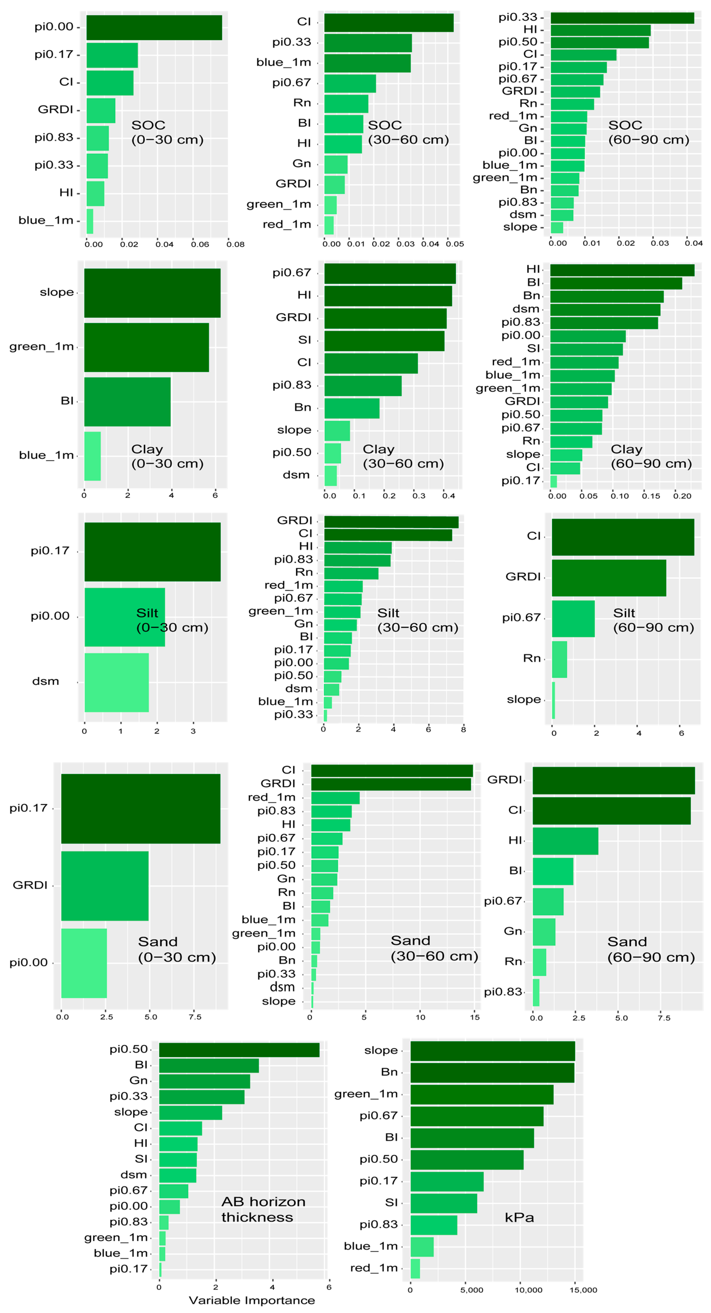
3.3. Variable Importance of Covariates

Figure 4 displays the selected covariates in the RF models after the RFE procedure and their importance. Depending on the target variable modeled, the number of covariates ranged from 3 to 18, indicating that all environmental variables were not important for predicting soil properties. Analysis revealed that OGC covariates were incorporated into all RF models, except for the topsoil clay content. OGC proved crucial for predicting SOC content at all depths, clay (30–60 cm), silt (30–60 cm), and sand (0–30 cm), as well as AB horizon thickness and penetration resistance. Among the UAV-based variables, the spectral indices CI, HI, BI, and GRDI emerged as the most influential covariates, whereas slope was the sole significant relief covariate for topsoil clay and penetration models.

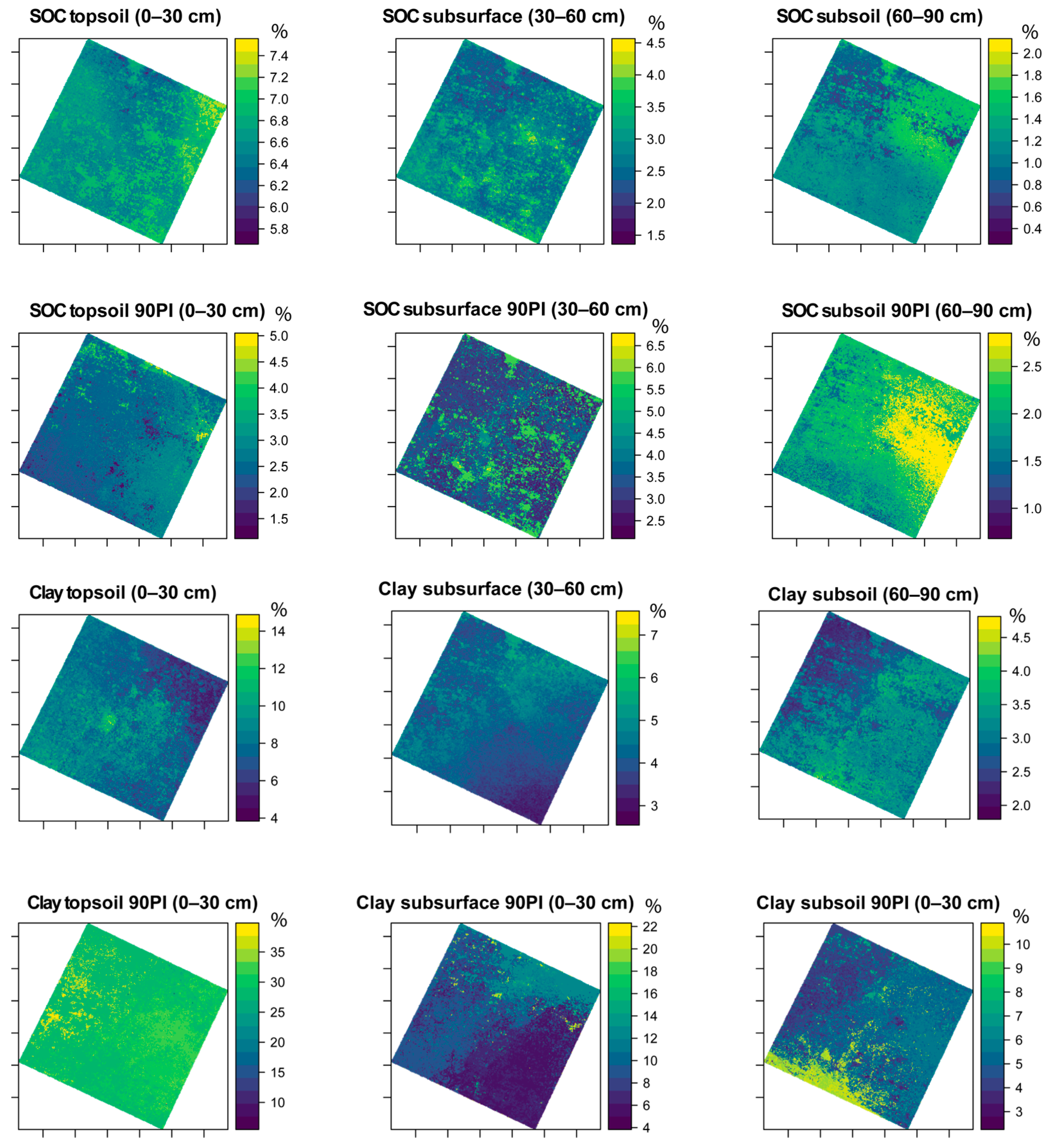
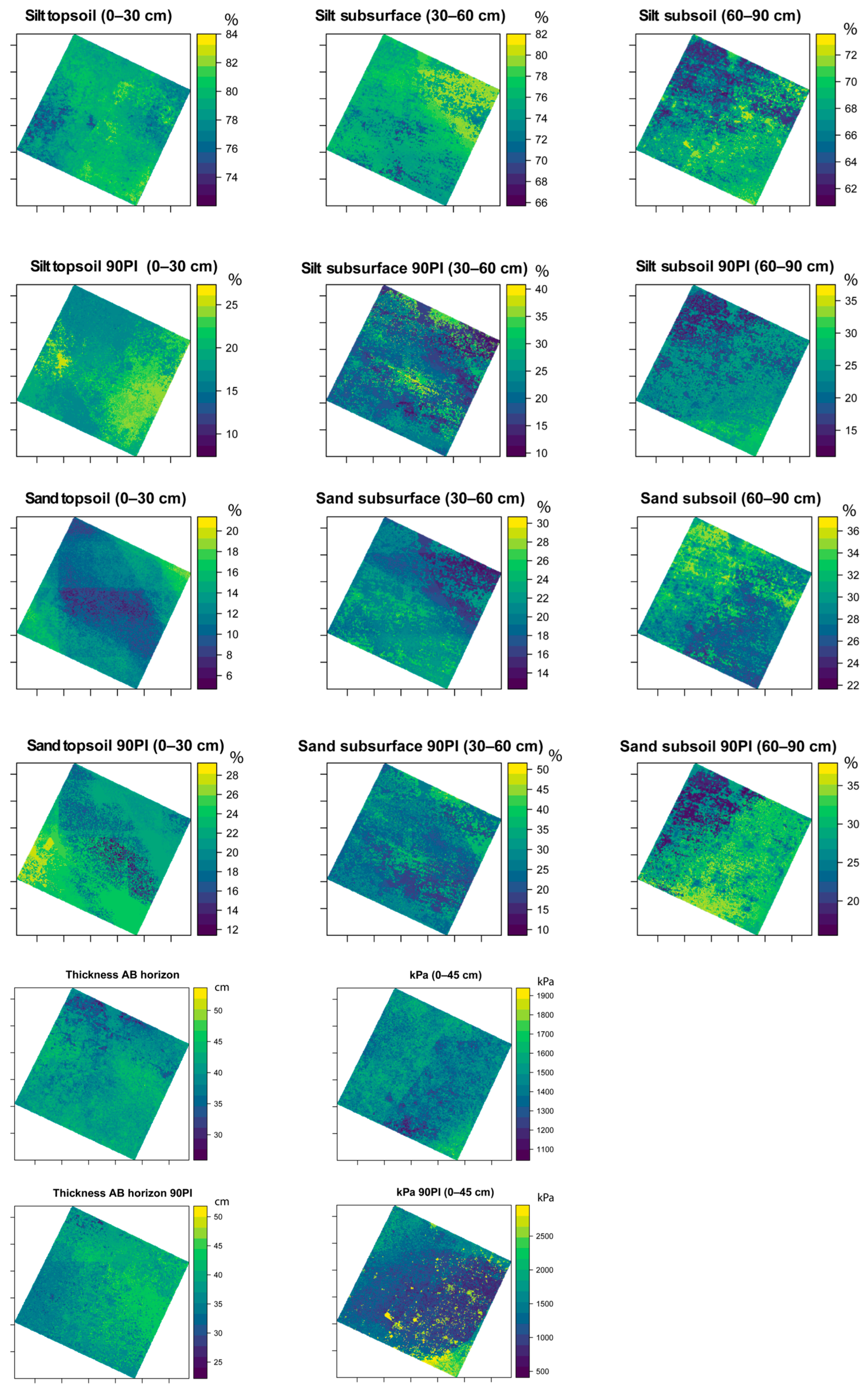
3.4. Spatial Predictions

The predicted values and associated uncertainties of soil properties based on the second scenario, which combined the UAV and OGC covariates, are presented in Figure 5. The topsoil and subsoil SOC maps were characterized by a similar spatial trend, where the highest levels were observed in the north-east part of the plot, whereas subsurface SOC had a patchy spatial structure. Soil texture maps displayed diverse patterns, with variations in content hotspots depending on depth. The lowest thicknesses of AB horizon were observed in the north-western part. The map of soil penetration resistance showed the highest kPa values in the eastern parts. The magnitude of uncertainty for each target variable was at a high level. In most cases, the highest uncertainty values are related to the highest predicted mean values.

4. Discussion

4.1. UAV Applicability

Our research indicates that the prediction of soil properties across several depths based on UAV images in a uniform site with a single vegetation type poses challenges. The successful prediction of a range of soil properties from remotely sensed data (UAV, airborne, spaceborne) is often achieved in scenarios where there is a clear spectral distinction between different soil types or where the landscape exhibits significant heterogeneity. This typically occurs in two main situations: (a) on croplands with a bare soil surface, or (b) in ecosystems with diverse plant communities or distinct land use types. Our study satisfied none of these conditions.

In the first case, accurate predictions of soil properties (mainly SOC and texture) in bare soils are primarily driven by the direct relationship between soil spectral signatures (dark or light colors) and these properties [16,39,40]. Hence, numerous studies showed encouraging outcomes for utilizing UAV-based data in predicting soil carbon [5,41,42] and texture [12] in bare soil, mainly in agricultural fields.

In landscapes with diverse vegetation or land use types, the spectral variations can be used as proxies for underlying soil properties [43,44]. In a review study by Lamichhane et al. [45], it was determined that at a farm- or plot-scale, land use and vegetation indices were the most important in predicting SOC. Similarly, Mahmoudabadi et al. [46] demonstrated that vegetation features and spectral indices were key in the modeling of several properties, including SOC, silt, and sand, across an over 1225 ha area using machine learning techniques.

4.2. Effect of Adding Spatial Position Variables

Our results demonstrated an improvement in the performance of prediction by adding OGC variables for most properties, although for some of them, they were negligible. As shown in previous studies that included spatial position covariates in machine learning soil models, their contribution can be different. In the study by Urbina-Salazar et al. [47], although such variables (latitude, longitude, and OGC) were not the most important ones for SOC modeling, they contributed to the prediction, i.e., they explained some variations in SOC content. A longitude covariate was the key to spatial predictions of soil thickness in central France [48], whereas spatial variables did not contribute to digital mapping of cropland soil pH [49]. Beyond geographic coordinates, potential spatial covariates can include variables that account for relationships between observations [22,23,50].

Nevertheless, creating spatially aware machine learning algorithms goes beyond simply including such predictors. There are numerous examples of hybrid machine learning methods that have combined with geostatistical methods. In such hybrid approaches, a machine learning algorithm is used to capture the deterministic spatial variation in soil properties, while kriging of the machine learning residuals models the stochastic component of variation [51]. For instance, RF combined with kriging of the residuals demonstrated better performance in soil mapping compared to machine learning or geostatistics predictive techniques [52,53,54].

As we demonstrated in this study, modeling soil properties under homogeneous vegetation conditions is not an easy task and it deserves special attention. Several studies have used hybrid methods to map soil parameters under these conditions. Ho et al. [55] modeled SOC density in Central Vietnamese tropical forests, using several approaches (geostatistics, machine learning, and their hybrid approaches) in combination with remote sensing data and other covariates. Results showed that the hybrid approaches achieved the best performance and demonstrated the most realistic spatial patterns of SOC density. Similar results appeared in other studies of relatively native forests, where hybrid methods produced the most accurate SOC stock predictions [53].

4.3. Variation of Soil Properties

There are six main soil-forming factors which affect soil properties: climate, time, vegetation and other life-forms, relief/topography, parent material, and anthropogenic impact [56]. The influence of climate and time are the same for the studied plot. The vegetation (species and height) also had a similar distribution within the investigated area, as did the topography (flat/leveled plateau with slight northwest exposure, i = 0.01–0.02). Therefore, we neglected the relief factor, which can influence the distribution of soil properties, but this can be considered as a limitation in the study and in prospects for further research (for example, using a LiDAR UAV). Many studies [57,58,59] indicated that the efficiency of soil properties’ prediction/modeling (using topography as the main covariate) is high mostly for undulating landscapes. However, Mosleh et al. [60] suggested that DSM could with sufficient accuracy also be applied for low-relief areas; Zhang et al. [61] proposed that surface soil properties can be accurately mapped by applying LiDAR. We assumed that the uneven distribution of soil properties on the studied plot is mainly due to the parent material (is represented by limestones [62]) and anthropogenic impact. It is well known that bedrock depth [63] and plowing [64] impact topsoil properties distribution and its content. The bedrock depth and humus-accumulative thickness varied within the study plot and had a heterogeneous distribution; also, before being abandoned, the territory was intensively plowed, which could have led to the movement of soil mass (tillage erosion).

5. Conclusions

While previous studies have shown promising results for predicting soil properties like carbon content using UAV imagery on bare soil, our results indicate that this approach is not readily transferable to sites with consistent vegetation cover. The uniform canopy masks the spectral variations associated with soil properties, making it difficult for machine learning models to distinguish them based on aerial imagery alone. Incorporating oblique geographic coordinates (OGCs) as covariates improved predictions for some variables, indicating the importance of considering spatial correlation in further studies. However, we supposed that the high variability of soil properties limited the importance of OGCs in the predictions. These findings should be considered when developing strategies for the spatial assessment of soil parameters using UAVs in agricultural lands.

To enhance spatial predictions of soil properties in homogeneous vegetation, the following steps should be considered: (i) accounting for the spatial autocorrelation and including geographic position as a covariate should not be ignored, so as to capture the spatial dependence of soil properties; (ii) utilizing multispectral and LiDAR UAV sensors to acquire soil-sensitive spectral bands; (iii) incorporating additional high-resolution covariates representing soil-forming factors; (iv) testing hybrid machine learning models that are based on a residual interpolation.

References

1. Arrouays, D.; McBratney, A.; Bouma, J.; Libohova, Z.; Richer-de-Forges, A.C.; Morgan, C.L.S.; Roudier, P.; Poggio, L.; Mulder, V.L. Impressions of digital soil maps: The good, the not so good, and making them ever better. Geoderma Reg. 2020, 20, e00255. [Google Scholar] [CrossRef]
2. Lozbenev, N.; Komissarov, M.; Zhidkin, A.; Gusarov, A.; Fomicheva, D. Comparative assessment of digital and conventional soil mapping: A case study of the Southern Cis-Ural region, Russia. Soil Syst. 2022, 6, 14. [Google Scholar] [CrossRef]
3. McBratney, A.B.; Mendonça Santos, M.L.; Minasny, B. On digital soil mapping. Geoderma 2003, 117, 3–52. [Google Scholar] [CrossRef]
4. Mulder, V.L.; de Bruin, S.; Schaepman, M.E.; Mayr, T.R. The use of remote sensing in soil and terrain mapping—A review. Geoderma 2011, 162, 1–19. [Google Scholar] [CrossRef]
5. Biney, J.K.M.; Houška, J.; Volánek, J.; Abebrese, D.K.; Cervenka, J. Examining the influence of bare soil UAV imagery combined with auxiliary datasets to estimate and map soil organic carbon distribution in an erosion-prone agricultural field. Sci. Total Environ. 2023, 870, 161973. [Google Scholar] [CrossRef]
6. Ding, M.; Li, X.; Jin, Z. Digital mapping of soil organic carbon using UAV images and soil properties in a thermo-erosion gully on the Tibetan Plateau. Remote Sens. 2023, 15, 1628. [Google Scholar] [CrossRef]
7. Zhou, J.; Xu, Y.; Gu, X.; Chen, T.; Sun, Q.; Zhang, S.; Pan, Y. High-precision mapping of soil organic matter based on UAV imagery using machine learning algorithms. Drones 2023, 7, 290. [Google Scholar] [CrossRef]
8. Zhang, C.; Kovacs, J.M. The application of small unmanned aerial systems for precision agriculture: A review. Precision Agric. 2012, 13, 693–712. [Google Scholar] [CrossRef]
9. Aldana-Jague, E.; Heckrath, G.; Macdonald, A.; van Wesemael, B.; Van Oost, K. UAS-based soil carbon mapping using VIS-NIR (480–1000 nm) multi-spectral imaging: Potential and limitations. Geoderma 2016, 275, 55–66. [Google Scholar] [CrossRef]
10. Reyes, J.; Wiedemann, W.; Brand, A.; Franke, J.; Ließ, M. Predictive monitoring of soil organic carbon using multispectral UAV imagery: A case study on a long-term experimental field. Spat. Inf. Res. 2024, 32, 683–696. [Google Scholar] [CrossRef]
11. Acharya, B.; Dodla, S.; Tubana, B.; Gentimis, T.; Rontani, F.; Adhikari, R.; Duron, D.; Bortolon, G.; Setiyono, T. Characterizing optimum N rate in waterlogged maize (Zea mays L.) with unmanned aerial vehicle (UAV) remote sensing. Agronomy 2025, 15, 434. [Google Scholar] [CrossRef]
12. Song, Q.; Gao, X.; Song, Y.; Li, Q.; Chen, Z.; Li, R.; Zhang, H.; Cai, S. Estimation and mapping of soil texture content based on unmanned aerial vehicle hyperspectral imaging. Sci. Rep. 2023, 13, 14097. [Google Scholar] [CrossRef] [PubMed]
13. Zeyliger, A.; Chinilin, A.; Ermolaeva, O. Spatial interpolation of gravimetric soil moisture using EM38-mk induction and ensemble machine learning (case study from dry steppe zone in Volgograd region). Sensors 2022, 22, 6153. [Google Scholar] [CrossRef] [PubMed]
14. Meinen, B.U.; Robinson, D.T. Agricultural erosion modelling: Evaluating USLE and WEPP field-scale erosion estimates using UAV time-series data. Environ. Model. Softw. 2021, 137, 104962. [Google Scholar] [CrossRef]
15. Peter, K.D.; d’Oleire-Oltmanns, S.; Ries, J.B.; Marzolff, I.; Ait Hssaine, A. Soil erosion in gully catchments affected by land-levelling measures in the Souss Basin, Morocco, analysed by rainfall simulation and UAV remote sensing data. Catena 2014, 113, 24–40. [Google Scholar] [CrossRef]
16. Gholizadeh, A.; Žižala, D.; Saberioon, M.; Borůvka, L. Soil organic carbon and texture retrieving and mapping using proximal, airborne and Sentinel-2 spectral imaging. Remote Sens. Environ. 2018, 218, 89–103. [Google Scholar] [CrossRef]
17. Vodyanitskii, Y.N.; Savichev, A.T. The influence of organic matter on soil color using the regression equations of optical parameters in the system CIE-L* a* b. Ann. Agrar. Sci. 2017, 15, 380–385. [Google Scholar] [CrossRef]
18. Nicolas, W.; Cecilia, C.; Hernán, A.; Mercedes, E.; Gastón, L.; Reussi Calvo, N.; Walter, C.; Sainz Rozas, H. The effect of agriculture on topsoil carbon stocks is controlled by land use, climate, and soil properties in the Argentinean Pampas. Catena 2022, 212, 106126. [Google Scholar] [CrossRef]
19. Paramesha, V.; Kumar, P.; Francaviglia, R.; Jyoti Nath, A.; Mishra, G.; Mohan Kumar, R.; Toraskar, S.; Rakhunde, S. Evaluating land use and climate change effects on soil organic carbon. A simulation study in coconut and pineapple systems in west coast India. Catena 2025, 248, 108587. [Google Scholar] [CrossRef]
20. Heuvelink, G.B.M.; Webster, R. Spatial statistics and soil mapping: A blossoming partnership under pressure. Spat. Stat. 2022, 50, 100639. [Google Scholar] [CrossRef]
21. Burgess, T.M.; Webster, R. Optimal interpolation and isarithmic mapping of soil properties: I The semi-variogram and punctual kriging. J. Soil Sci. 1980, 31, 315–331. [Google Scholar] [CrossRef]
22. Behrens, T.; Schmidt, K.; Viscarra Rossel, R.; Gries, P.; Scholten, T.; Macmillan, R.A. Spatial modelling with Euclidean distance fields and machine learning. Eur. J. Soil Sci. 2018, 69, 757–770. [Google Scholar] [CrossRef]
23. Hengl, T.; Nussbaum, M.; Wright, M.N.; Heuvelink, G.B.M.; Gräler, B. Random forest as a generic framework for predictive modeling of spatial and spatio-temporal variables. PeerJ 2018, 6, e5518. [Google Scholar] [CrossRef]
24. Møller, A.B.; Beucher, A.M.; Pouladi, N.; Greve, M.H. Oblique geographic coordinates as covariates for digital soil mapping. SOIL 2020, 6, 269–289. [Google Scholar] [CrossRef]
25. Chen, Z.; Wang, Z.; Wang, X.; Shi, Z.; Chen, S. Including soil spatial neighbor information for digital soil mapping. Geoderma 2024, 451, 117072. [Google Scholar] [CrossRef]
26. Peel, M.C.; Finlayson, B.L.; McMahon, T.A. Updated world map of the Köppen-Geiger climate classification. Hydrol. Earth Syst. Sci. 2007, 11, 1633–1644. [Google Scholar] [CrossRef]
27. Baisheva, E.; Fedorov, N.; Zhigunova, S.N.; Shirokikh, P.; Komissarov, M.; Gabbasova, I.; Muldashev, A.; Bikbaev, I.; Tuktamyshev, I.; Shendel, G.; et al. Productivity of vegetation and carbon stock in meadow steppe on fallow areas in the Bashkir Cis-Urals (Southern Urals region), Russia. South Russ. Ecol. Dev. 2023, 18, 64–73. [Google Scholar] [CrossRef]
28. IUSS Working Group WRB. World Reference Base for Soil Resources. In International Soil Classification System for Naming Soils and Creating Legends for Soil Maps, 4th ed.; International Union of Soil Sciences (IUSS): Vienna, Austria, 2022; ISBN 9798986245119. [Google Scholar]
29. State Standard of the USSR 26213-91. Soils. Methods for Determination of Organic Matter. 1993. Available online: http://docs.cntd.ru/document/1200023481 (accessed on 21 September 2022).
30. Walldey, A.; Black, I.A. Estimation of soil organic carbon by the chromic acid titration method. Soil Sci. 1934, 47, 29–38. [Google Scholar]
31. Hijmans, R.J. Terra: Spatial Data Analysis; R Package Version 1.5-21; 2022. Hijmans, R. terra: Spatial Data Analysis. R Package Version 1.8-44. 2025. Available online: https://github.com/rspatial/terra (accessed on 18 March 2025).
32. Kawashima, S.; Nakatani, M. An algorithm for estimating chlorophyll content in leaves using a video camera. Ann. Bot. 1998, 81, 49–54. [Google Scholar] [CrossRef]
33. Levin, N.; Ben-Dor, E.; Singer, A. A digital camera as a tool to measure colour indices and related properties of sandy soils in semi-arid environments. Int. J. Remote Sens. 2005, 26, 5475–5492. [Google Scholar] [CrossRef]
34. Tucker, C.J. Red and Photographic infrared linear combinations for monitoring vegetation. Remote Sens. Environ. 1979, 8, 127–150. [Google Scholar] [CrossRef]
35. Breiman, L. Random forests. Mach. Learn. 2001, 45, 5–32. [Google Scholar] [CrossRef]
36. Gregorutti, B.; Michel, B.; Saint-Pierre, P. Correlation and variable importance in random forests. Stat. Comput. 2017, 27, 659–678. [Google Scholar] [CrossRef]
37. Kuhn, M. Building Predictive models in R using the caret Package. J. Stat. Software 2008, 28, 1–26. [Google Scholar] [CrossRef]
38. Meinshausen, N. Quantile regression forests. J. Mach. Learn. Res. 2006, 7, 983–999. [Google Scholar]
39. Castaldi, F.; Hueni, A.; Chabrillat, S.; Ward, K.; Buttafuoco, G.; Bomans, B.; Vreys, K.; Brell, M.; van Wesemael, B. Evaluating the capability of the Sentinel 2 data for soil organic carbon prediction in croplands. J. Photogramm. Remote Sens. 2019, 147, 267–282. [Google Scholar] [CrossRef]
40. Suleymanov, A.; Suleymanov, R.; Gabbasova, I.; Saifullin, I. Field-scale digital mapping of top- and subsoil Chernozem properties. Precision Agric. 2024, 25, 1636–1657. [Google Scholar] [CrossRef]
41. Heil, J.; Jörges, C.; Stumpe, B. Fine-scale mapping of soil organic matter in agricultural soils using UAVs and machine learning. Remote Sens. 2022, 14, 3349. [Google Scholar] [CrossRef]
42. Zhang, H.; Shi, P.; Crucil, G.; van Wesemael, B.; Limbourg, Q.; Oost, K.V. Evaluating the capability of a UAV-borne spectrometer for soil organic carbon mapping in bare croplands. Land Degrad. Dev. 2021, 32, 4375–4389. [Google Scholar] [CrossRef]
43. Rasel, S.M.M.; Groen, T.A.; Hussin, Y.A.; Diti, I.J. Proxies for soil organic carbon derived from remote sensing. Int. J. Appl. Earth Obs. Geoinf. 2017, 59, 157–166. [Google Scholar] [CrossRef]
44. Suleymanov, A.; Abakumov, E.; Alekseev, I.; Nizamutdinov, T. Digital mapping of soil properties in the high latitudes of Russia using sparse data. Geoderma Reg. 2024, 36, e00776. [Google Scholar] [CrossRef]
45. Lamichhane, S.; Kumar, L.; Wilson, B. Digital soil mapping algorithms and covariates for soil organic carbon mapping and their implications: A review. Geoderma 2019, 352, 395–413. [Google Scholar] [CrossRef]
46. Mahmoudabadi, E.; Karimi, A.; Haghnia, G.H.; Sepehr, A. Digital soil mapping using remote sensing indices, terrain attributes, and vegetation features in the rangelands of Northeastern Iran. Environ. Monit. Assess. 2017, 189, 500. [Google Scholar] [CrossRef] [PubMed]
47. Urbina-Salazar, D.; Vaudour, E.; Richer-de-Forges, A.C.; Chen, S.; Martelet, G.; Baghdadi, N.; Arrouays, D. Sentinel-2 and Sentinel-1 bare soil temporal mosaics of 6-Year periods for soil organic carbon content mapping in Central France. Remote Sens. 2023, 15, 2410. [Google Scholar] [CrossRef]
48. Chen, S.; Richer-de-Forges, A.C.; Leatitia Mulder, V.; Martelet, G.; Loiseau, T.; Lehmann, S.; Arrouays, D. Digital mapping of the soil thickness of loess deposits over a calcareous bedrock in Central France. Catena 2021, 198, 105062. [Google Scholar] [CrossRef]
49. Chen, J.; Xie, E.; Peng, Y.; Yan, G.; Jiang, J.; Hu, W.; Zhao, Y.; Saifullah Khan, K.; Zhao, Y. Four-dimensional modelling reveals decline in cropland soil pH during last four decades in China’s Mollisols region. Geoderma 2025, 453, 11713. [Google Scholar] [CrossRef]
50. Sekulić, A.; Kilibarda, M.; Heuvelink, G.B.M.; Nikolić, M.; Bajat, B. Random forest spatial interpolation. Remote Sens. 2020, 12, 1687. [Google Scholar] [CrossRef]
51. Keskin, H.; Grunwald, S. Regression kriging as a workhorse in the digital soil mapper’s toolbox. Geoderma 2018, 326, 22–41. [Google Scholar] [CrossRef]
52. Guo, P.-T.; Li, M.-F.; Luo, W.; Tang, Q.-F.; Liu, Z.-W.; Lin, Z.-M. Digital mapping of soil organic matter for rubber plantation at regional scale: An application of random forest plus residuals kriging approach. Geoderma 2015, 237–238, 49–59. [Google Scholar] [CrossRef]
53. Suleymanov, A.; Abakumov, E.; Nizamutdinov, T.; Polyakov, V.; Shevchenko, E.; Makarova, M. Soil organic carbon stock retrieval from Sentinel-2A using a hybrid approach. Environ. Monit. Assess. 2023, 196, 23. [Google Scholar] [CrossRef]
54. Wang, L.; Wu, W.; Liu, H.-B. Digital mapping of topsoil pH by random forest with residual kriging (RFRK) in a hilly region. Soil Res. 2019, 57, 387–396. [Google Scholar] [CrossRef]
55. Ho, V.H.; Morita, H.; Ho, T.H.; Bachofer, F.; Nguyen, T.T. Comparison of geostatistics, machine learning algorithms, and their hybrid approaches for modeling soil organic carbon density in tropical forests. J. Soils Sediments 2025, 1–24. [Google Scholar] [CrossRef]
56. Jenny, H. Factors of Soil Formation: A System of Quantitative Pedology; Courier Corporation: Chelmsford, MA, USA, 1994; 281p. [Google Scholar]
57. Manning, G.; Fuller, L.G.; Eilers, R.G.; Florinsky, I. Topographic influence on the variability of soil properties within an undulating Manitoba landscape. Can. J. Soil Sci. 2001, 81, 439–447. [Google Scholar] [CrossRef]
58. Sharma, S.; Swami, D. Elevation-dependent dynamics of soil properties in a hilly watershed: A landform-based approach. Environ. Monit. Assess. 2024, 196, 1001. [Google Scholar] [CrossRef]
59. Jiao, P.; Ou, Y.; Pang, S.; Yan, B.; Zhang, Y.; Xu, W.; Yan, L. Impacts of landscape factors on gully retreat and its morphological characteristics in hilly areas of Northeast China. Soil Till. Res. 2025, 248, 106434. [Google Scholar] [CrossRef]
60. Mosleh, Z.; Salehi, M.H.; Jafari, A.; Borujeni, I.E.; Mehnatkesh, A. The effectiveness of digital soil mapping to predict soil properties over low-relief areas. Environ. Monit. Assess. 2016, 188, 195. [Google Scholar] [CrossRef]
61. Zhang, Y.; Hartemink, A.E.; Huang, J.; Townsend, P.A. Synergistic use of hyperspectral imagery, Sentinel-1 and LiDAR improves mapping of soil physical and geochemical properties at the farm-scale. Eur. J. Soil Sci. 2021, 72, 1690–1717. [Google Scholar] [CrossRef]
62. Baisheva, E.Z.; Bikbaev, I.G.; Martynenko, V.B.; Shirokikh, P.S.; Naumova, L.G. Bryophyte diversity of calcareous fens in the Bashkir Cis-Urals (Republic of Bashkortostan, the Southern Urals). KnE Life Sci. 2018, 19–25. [Google Scholar]
63. Hopp, L.; McDonnell, J.J. Connectivity at the hillslope scale: Identifying interactions between storm size, bedrock permeability, slope angle and soil depth. J. Hydrol. 2009, 376, 378–391. [Google Scholar] [CrossRef]
64. Komissarov, M.A.; Klik, A. The impact of no-till, conservation, and conventional tillage systems on erosion and soil properties in Lower Austria. Eurasian Soil Sci. 2020, 53, 503–511. [Google Scholar] [CrossRef]
Figure 1. The location of the Republic of Bashkortostan (image source—Google maps) (a); the investigation area (steppe site) and elevation map (b); and UAV-based natural color imagery with the sample points (c).
Land 14 00931 g001
Figure 2. A view of the studied plot (the azimuth of the photo 185°) (a); soil cross-section #1 (b); soil sampling; measuring of humus-accumulative horizon (A + AB) thickness (sample point #44) (c); and DJI Phantom 4 RTK drone (d).
Land 14 00931 g002
Figure 3. Examples of OGC covariates. The covariates (a,d) are equivalent to the x and y coordinates, respectively. The covariates (b,c,e,f) are coordinates at oblique angles.
Land 14 00931 g003
Figure 4. Relative importance of covariates in the RF models (a darker shade corresponds to a higher importance of the variable).
Land 14 00931 g004
Figure 5. Predicted mean values of soil properties for each depth interval (top row) and 90% prediction interval width (bottom row).
Land 14 00931 g005aLand 14 00931 g005b