Analysis and Prediction of Spatial and Temporal Land Use Changes in the Urban Agglomeration on the Northern Slopes of the Tianshan Mountains

Abstract

This study investigates the spatiotemporal changes in land use within the urban agglomeration on the northern slopes of the Tianshan Mountains (TNUA), aiming to identify the driving factors and provide a scientific basis for regional ecological protection, rational land use planning, and sustainable resource utilization. Using land use data, we analyzed transitions, dynamics, intensity, and gravity shifts in land use, examined driving mechanisms using geographic detectors, and simulated future land use patterns with the Patch-generating Land Use Simulation (PLUS) model. The results indicate that between 2010 and 2020, forest, water body, and unused land areas decreased, while cropland, grassland, and construction land expanded. The rate of land use change accelerated significantly, increasing from 0.0955% during 2010–2015 to 0.3192% during 2015–2020. The comprehensive land use dynamic degree index rose from 157.8371 to 161.1008, with Shayibake District exhibiting the most rapid growth. Precipitation, temperature, economic development, and elevation were the dominant driving factors throughout the study period. Population density had the strongest influence on the expansion of water body, while slope was the most significant factor for cropland expansion. Nighttime light was the primary driver of construction land growth. Projections for 2025, 2030, and 2035 suggest a continued decline in unused land and forest areas, alongside increases in cropland, grassland, water body, and construction land.

1. Introduction

Urban agglomerations are the core areas of new urbanization, playing an important role in land use change. They clearly illustrate the ecological changes and unique characteristics arising from the interaction between human activities and the natural environment. Urbanization profoundly impacts the local environment and natural resources through land use change [1]. As the core area of Xinjiang’s economic development, the urban agglomeration on the northern slopes of the Tianshan Mountains (TNUA) has received considerable attention since the Belt and Road Initiative and plays a strategic role in stabilizing Xinjiang and maintaining national unity [2]. Since the Belt and Road Initiative was proposed in 2013, it has profoundly influenced regional development. This study selects 2010 as the base year before the policy implementation and combines 2015 and 2020 data to (1) analyze land use transitions in TNUA during 2010–2020, and (2) examine the driving mechanisms through geographic detectors. The findings provide scientific references for promoting harmonious economic–ecological development in TNUA.

The nature of land use change reflects the interactive processes between human activities and natural systems. Ellis et al. [3] systematically demonstrated the profound impacts of human agricultural civilization on land use from a macro-historical perspective, integrating archaeological evidence, paleoecological data, environmental history, and model-based reconstructions. At the regional scale, Nébié et al. [4] applied a political ecology framework to investigate land use/land cover changes in Burkina Faso (1975–2013) by combining time-series remote sensing data, census records, and local oral histories, revealing that population migration substantially altered land use patterns: cropland expanded markedly in immigration zones, whereas forest and grassland regenerated in emigration areas. Mosofe et al. [5] established that wetland degradation in Tanzania correlates significantly with population growth, urban expansion, and policy reforms through random forest algorithms and bibliometric analysis. Chisanga et al. [6] quantified Zambia’s wetland degradation over two decades using multi-temporal remote sensing data, identifying urban and agricultural encroachment as primary drivers of land cover transformation. These studies collectively characterize spatiotemporal land use change patterns and provide a foundation for analyzing driving mechanisms and predictive modeling.

Following the characterization of land use changes, numerous studies have focused on analyzing their driving factors. Lambin et al. [7] systematically synthesized the causes of land use changes from a macro perspective as early as 2001, identifying key drivers, including population growth, economic development, and policy adjustments, while highlighting the regional variability and multifactorial nature of these mechanisms. Through systematic review and bibliometric analysis, Allan et al. [8] demonstrated that contemporary research has evolved from examining isolated natural and social variables toward multi-scale coupled analyses. This reflects the paradigm shift in land use change studies, from static driver identification to dynamic mechanism modeling. Wu et al. [9] developed a marginal metric method based on random forest algorithms to identify core drivers of urban land use change. Utilizing multi-temporal global land cover products and point-of-interest (POI) data for Wuhan (2010–2020), they identified transportation infrastructure, population density, and commercial activity density as primary determinants. Complementary studies by Peng et al. [10] and Zhang et al. [11] examined land use transitions in Wuhan and Xi’an respectively through the lens of ecosystem service values, revealing the complex interplay between human demands, policy interventions, and ecological constraints underlying land conversion processes. Collectively, these advances in dynamic mechanism analysis have established a robust foundation for land use change simulation and prediction.

Having established the research foundation of land use change trends and driving mechanisms, the simulation and prediction of future land use patterns has become a crucial research focus. Pijanowski et al. [12] pioneered the integration of geographic information systems (GIS) with artificial neural network (ANN)-based Land Transformation Models (LTM) for predictive modeling as early as 2002. Gharaibeh et al. [13] enhanced the simulation capability by incorporating ANN into Cellular Automata-Markov Chain (CA-MC) models, demonstrating that considering driving forces significantly improves prediction accuracy and better represents nonlinear land use changes, particularly in peri-urban transition zones. To address complex urban expansion and ecological evolution processes, Doelman et al. [14] employed the IMAGE model to analyze land use dynamics under Shared Socioeconomic Pathways (SSPs), generating both regional and gridded projections that expanded the policy applications of land system modeling in global change studies. Leta et al. [15] applied the Land Change Modeler (LCM) with a Multilayer Perceptron Neural Network-Cellular Automata-Markov Chain (MLPNN-CA-MC) approach in Ethiopia’s Nashe water body, noting the model’s limited responsiveness to policy guidance and recommending stronger integration of social driving mechanisms. Koko et al. [16] implemented a hybrid CA-Markov model in Nigeria’s Kano metropolitan area, highlighting the challenges of maintaining model accuracy in rapidly urbanizing regions. Avtar et al. [17] projected 2040 land use patterns for Fiji’s Viti Levu Island using Cellular Automata-Artificial Neural Network (CA-ANN) modeling, complemented by InVEST model analysis of carbon sequestration and economic values across three time periods (2000, 2020, and 2040). The recently developed PLUS model (Liang et al. [18]) combines stochastic seeding mechanisms with probabilistic land expansion inference through two innovative modules: (1) the Land Expansion Analysis Strategy (LEAS) module, which analyzes historical land change drivers to generate transition probability maps, and (2) the Cellular Automata based on Random Seeds (CARS) module, which simulates spatial expansion patterns. This framework effectively addresses traditional CA model limitations regarding irregular parcel shapes and discontinuous changes while supporting multi-scenario simulations, particularly demonstrating superior accuracy in modeling urban expansion dynamics and showing strong regional adaptability for applications in urban agglomeration research and ecological conservation planning.

In summary, while existing studies have examined land use transitions and their driving factors, comprehensive methodologies remain limited [8]. Most analyses rely on qualitative approaches, with quantitative studies being less common. Furthermore, TNUA has been understudied despite its ecological and economic importance. Predicting land use patterns in this region is critical for ecological protection and sustainable development. This study provides two key contributions: (1) a comprehensive analysis of land use transitions in TNUA using transfer matrices, dynamic degree indices, intensity analysis, and gravity shift modeling, combined with geographic detector analysis to quantify driving mechanisms; (2) application of the PLUS model to simulate future land use patterns, offering scientific support for regional planning and conservation.

2. Materials and Methods

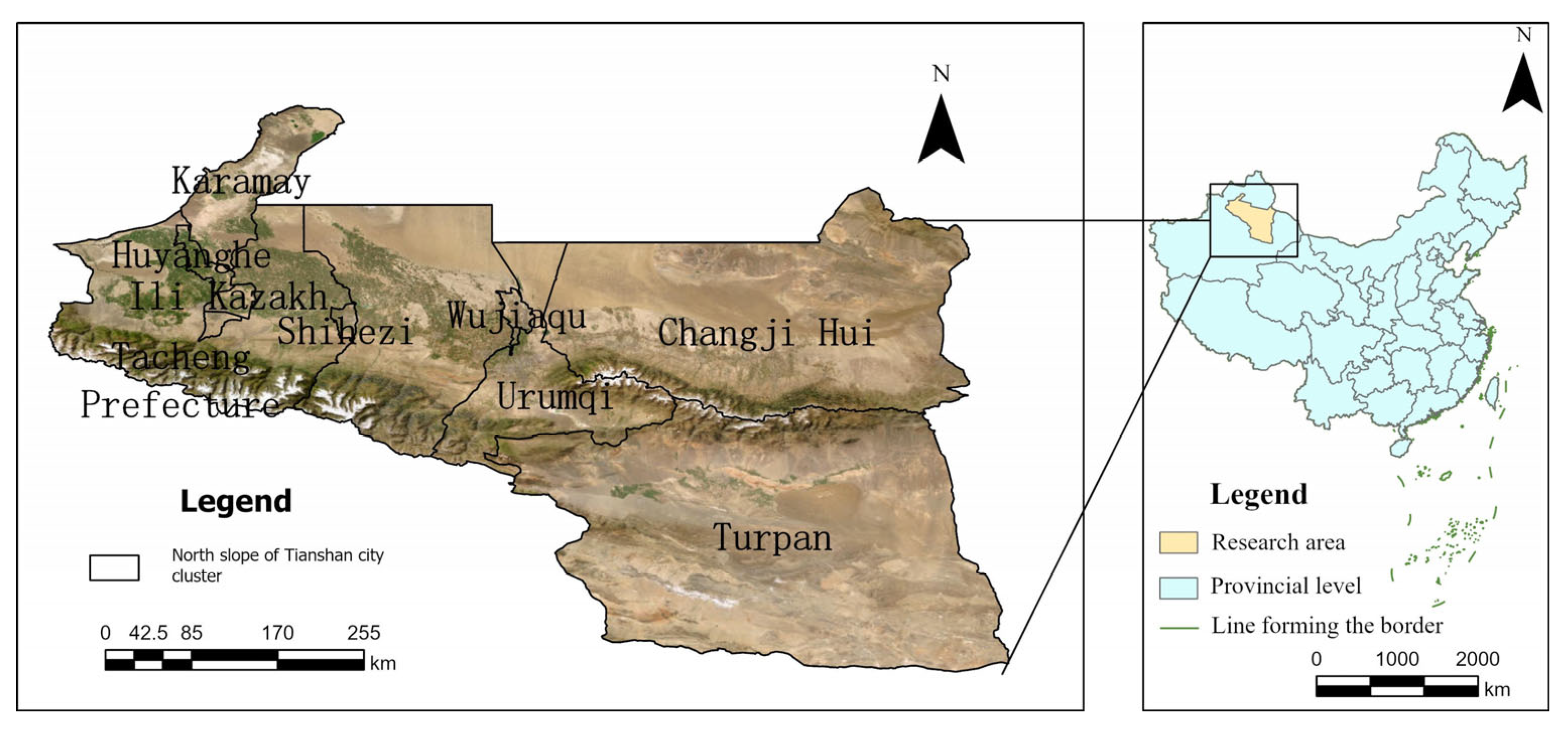
2.1. Overview of the Study Area

TNUA is located in the Xinjiang Uygur Autonomous Region at the northern foothills of the Tianshan Mountains (42°75′–49°59′ N, 81°30′–93°33′ E). The region exhibits a pronounced south-to-north topographic gradient, featuring three distinct geomorphological units: mountainous terrain, alluvial plains, and desert transition zones. Characterized by a temperate continental arid to semi-arid climate, the area experiences mean annual temperatures of 6–9 °C with precipitation ranging from 200–500 mm, while evaporation rates significantly exceed precipitation levels, resulting in limited water availability. Natural vegetation displays clear vertical zonation, with desert and grassland ecosystems predominating at lower elevations, artificial oasis agriculture dominating the central plains, and montane meadows with coniferous forests occurring at higher altitudes. Geographically, the region occupies a strategic transitional zone along the central northern slopes of the Tianshan Mountains, adjacent to the southern margin of the Junggar Basin. TNUA is one of the 19 key urban agglomerations officially proposed by China’s National Development and Reform Commission in 2016, and we follow the usual name of TNUA and denote the scope of TNUA by all the administrative boundaries of the cities it contains, which is the scope of the study area of this study [19]. The administrative divisions of TNUA are shown in Figure 1.

With a total area of 95,400 km² (5.7% of Xinjiang’s total) and a population of 4.58 million (23.3% of Xinjiang’s population), TNUA serves as the economic, social, and technological hub of Xinjiang. This strategically vital region exhibits an 86.98% urbanization rate, and 83% of Xinjiang’s heavy industry and 62% of its light industry are concentrated in this area. As a pivotal zone for China’s Great Northwest Development Strategy, TNUA holds particular importance for the Belt and Road Initiative and China’s western opening policy. The region possesses abundant natural resources, including Xinjiang’s richest deposits of coal, petroleum, and natural gas. Situated in the Tianshan piedmont snowmelt zone, TNUA maintains relatively concentrated water resources through its river networks despite the arid climate. Furthermore, the area’s exceptional solar energy potential stems from abundant light and heat resources. The diverse landscapes, rich biodiversity, and unique tourism assets further enhance its developmental potential. These combined resources provide optimal conditions for sustainable regional development.

2.2. Data Sources

The data sources used in this study are presented in

Table 1. Data sources.

Data	Source	Resolution	Time
LULC	Resource and Environmental Science Data Center (https://www.resdc.cn, accessed on 10 May 2024)	30 m	2010, 2015, 2020
DEM	NASADEM (https://search.earthdata.nasa.gov/search, accessed on 8 March 2024)	30 m	2010, 2015, 2020
Temperature	National Earth System Science Data Center, National Science & Technology Infrastructure of China (http://www.geodata.cn, accessed on 10 May 2024)	1 km	2010, 2015, 2020
Precipitation	National Earth System Science Data Center, National Science & Technology Infrastructure of China (http://www.geodata.cn, accessed on 10 May 2024)	1 km	2010, 2015, 2020
Nighttime Light	Dataset produced by Li et al. [21].	1 km	2010, 2015, 2020
Population	LandScan (https://landscan.ornl.gov, accessed on 5 April 2024)	1 km	2010, 2015, 2020
Population Density	SEDAC (http://sedac.ciesin.columbia.edu/data/sets/browse, accessed on 5 April 2024)	1 km	2010, 2015, 2020
GDP	Resource and Environmental Science Data Center (http://www.resdc.cn, accessed on 10 May 2024)	1 km	2010, 2015, 2020

. Following the classification system established by the Resource and Environment Science and Data Center (RESDC) of the Chinese Academy of Sciences, we categorized land use types from the China Land Use/Cover Change dataset (CNLUCC) into six classes: (1) cropland, (2) forest, (3) grassland, (4) water body, (5) construction land, and (6) unused land. Using spatial analysis tools, we derived slope and aspect information from digital elevation data.

The nighttime light data were produced by Li et al. [21]. Through comprehensive global statistical analyses and regional case studies (including urban areas in China and the United States), their study demonstrated that the fused dataset maintains high consistency with original observations in brightness distribution, spatial structure, and temporal trends, confirming its accuracy and reliability. This dataset has been widely applied in research requiring high precision, including urban expansion monitoring, economic activity assessment, and energy consumption estimation, attesting to its scientific and practical value. LandScan data provide estimates of total population derived from a dynamic distribution model that integrates multiple data sources, with particular strength in capturing cross-administrative boundary population patterns. In contrast, SEDAC data offer average population density calculated by dividing population counts by areal extent. While total population data help characterize the aggregate effects of population concentration on land use changes across urban agglomerations, population density data elucidate the relationship between spatial clustering intensity and land expansion heterogeneity. We conducted rigorous quality control to ensure temporal consistency (2010, 2015, 2020) and uniform spatial resolution (1 km) for all datasets, thereby guaranteeing the scientific validity of our integrated analysis.

2.3. Research Methodology

2.3.1. Land Use Transfer Matrix

The land use transfer matrix serves as a fundamental analytical tool for quantifying land use changes during a specified time period within a study area. This method constructs a two-dimensional matrix that systematically compares land use classifications at different temporal points for identical spatial locations. Through matrix analysis, researchers can precisely quantify both the magnitude and spatial patterns of land type conversions across the study region. The mathematical representation of this matrix is expressed as follows:

$$\mathrm{S}=\left(\begin{array}{ccc}{\mathrm{S}}_{11}& \dots & {\mathrm{S}}_{1\mathrm{n}}\\ ⋮& \ddots & ⋮\\ {\mathrm{S}}_{1\mathrm{n}}& \dots & {\mathrm{S}}_{\mathrm{n}\mathrm{n}}\end{array}\right)$$

(1)

where S represents the land use area and n denotes the number of land use types.

Compared with traditional change detection methods based on spectral information (e.g., image differencing), the land use transfer matrix utilizes classification results to quantitatively analyze transition relationships between different land use types. This approach explicitly identifies both the conversion pathways (i.e., which land use types are transformed into others) and the corresponding areal magnitudes. Consequently, it provides a robust scientific foundation for examining structural patterns and driving mechanisms underlying land use changes.

2.3.2. Land Use Dynamics

The average annual rate of change (${\mathrm{K}}_{\mathrm{i}}$) quantifies the transformation rate of a specific land use type within the study area during a given period. This metric enables systematic analysis of both the pace and scale of land use changes across TNUA. The comprehensive land use dynamic degree (s) characterizes the overall land use change intensity for the entire region, facilitating comparative studies of spatial heterogeneity in land use dynamics. The mathematical expressions are defined as follows:

$${\mathrm{K}}_{\mathrm{i}}={\displaystyle \frac{{\mathrm{S}}_{\mathrm{i}\mathrm{t}2}-{\mathrm{S}}_{\mathrm{i}\mathrm{t}1}}{{\mathrm{S}}_{\mathrm{i}\mathrm{t}1}}}\times {\displaystyle \frac{1}{{\mathrm{t}}_2-{\mathrm{t}}_1}}\times 100\%$$

(2)

$$\mathrm{s}=\left({\sum }_{\mathrm{i}=1}^{\mathrm{n}}{\displaystyle \frac{△{\mathrm{S}}_{\mathrm{i}-\mathrm{j}}}{{\mathrm{S}}_{\mathrm{i}}}}\right)\times {\displaystyle \frac{1}{\mathrm{t}}}\times 100\%$$

(3)

where ${\mathrm{K}}_{\mathrm{i}}$ represents the dynamic degree of land use type i over the time period from ${\mathrm{t}}_1$ to ${\mathrm{t}}_2$; ${\mathrm{S}}_{\mathrm{i}\mathrm{t}1}$ and ${\mathrm{S}}_{\mathrm{i}\mathrm{t}2}$ denote the areas of land use type i at times points ${\mathrm{t}}_1$ and ${\mathrm{t}}_2$, respectively; ${\mathrm{S}}_{\mathrm{i}-\mathrm{j}}$ indicates the area converted from land use type i to other types during the study period; ${\mathrm{S}}_{\mathrm{i}}$ corresponds to the area of land use type i at the study period’s end; and t signifies the total study duration.

2.3.3. Land Use Intensity

Land use intensity quantifies the extent of human utilization and development of land resources within a defined geographical area. A higher index value indicates greater land development intensity. This metric reflects both the magnitude and patterns of human-land interactions within the study region. The composite land use intensity index and its temporal change metric are calculated as follows:

$$\mathrm{I}=100\sum _{\mathrm{i}=1}^{\mathrm{n}}{\mathrm{A}}_{\mathrm{i}}\mathrm{I}{\mathrm{C}}_{\mathrm{i}}$$

(4)

$$△{\mathrm{I}}_{\mathrm{b}-\mathrm{a}}={\mathrm{I}}_{\mathrm{b}}-{\mathrm{I}}_{\mathrm{a}}=\left(\sum _{\mathrm{i}=1}^{\mathrm{n}}{\mathrm{A}}_{\mathrm{i}}\times {\mathrm{C}}_{\mathrm{i}\mathrm{b}}-\sum _{\mathrm{i}=1}^{\mathrm{n}}{\mathrm{A}}_{\mathrm{i}}\times {\mathrm{C}}_{\mathrm{i}\mathrm{a}}\right)\times 100\%$$

(5)

where I represents the composite land use intensity index for the study area; ${\mathrm{A}}_{\mathrm{i}}$ denotes the graded intensity index for level i; ${\mathrm{C}}_{\mathrm{i}}$ indicates the areal percentage of land use intensity level i; ${\mathrm{I}}_{\mathrm{b}-\mathrm{a}}$ quantifies the temporal change in composite intensity between periods a and b; ${\mathrm{I}}_{\mathrm{a}}$ and ${\mathrm{I}}_{\mathrm{b}}$ correspond to the composite indices at respective time points; and ${\mathrm{C}}_{\mathrm{i}\mathrm{a}}$ and ${\mathrm{C}}_{\mathrm{i}\mathrm{b}}$ specify the areal percentages of level i at times a and b.

2.3.4. Gravity Center Shift Analysis

The gravity center represents the spatial distribution centroid of a specific land use type within a geographic coordinate system. The gravity center shift quantifies the positional displacement of this centroid across different time periods. This analytical approach enables systematic examination of spatiotemporal distribution changes for individual land use categories within the study area. Through gravity center trajectory analysis, we can visually characterize the spatial expansion and migration patterns of land use types in TNUA over time. The centroid coordinates are calculated as follows:

$$\mathrm{X}=\sum _{\mathrm{i}=1}^{\mathrm{n}}{\mathrm{x}}_{\mathrm{i}}{\mathrm{M}}_{\mathrm{i}}/\sum _{\mathrm{i}=1}^{\mathrm{n}}{\mathrm{M}}_{\mathrm{i}}$$

(6)

$$\mathrm{Y}=\sum _{\mathrm{i}=1}^{\mathrm{n}}{\mathrm{y}}_{\mathrm{i}}{\mathrm{M}}_{\mathrm{i}}/\sum _{\mathrm{i}=1}^{\mathrm{n}}{\mathrm{M}}_{\mathrm{i}}$$

(7)

where X and Y are the longitude and latitude coordinates of the gravity center. The variables ${\mathrm{x}}_{\mathrm{i}}$ and ${\mathrm{y}}_{\mathrm{i}}$ denote the geographic coordinates of the centroid in the i-th subregion, while ${\mathrm{M}}_{\mathrm{i}}$ quantifies the attribute magnitude in the corresponding subregion. Through systematic computation of these parameters, we can precisely determine the spatial position of the attribute-specific gravity center.

2.3.5. Geodetector

The Geodetector method [22], developed by researchers at the Chinese Academy of Sciences, is a spatial statistical analysis tool designed to identify geospatial stratified heterogeneity and its driving factors. This method provides four analytical functions: (1) factor detection, (2) interaction detection, (3) risk zone detection, and (4) ecological detection. In this study, we apply factor detection and interaction detection to analyze the driving mechanisms of land use transitions in the study area.

(1)

Factor Detection

Factor detection quantifies the spatial heterogeneity of land use change (dependent variable Y) and evaluates the explanatory power of driving factor X on the observed spatial patterns. This module identifies the primary determinants influencing land use transitions in TNUA. The statistical model is expressed as:

$$\mathrm{q}=1-{\displaystyle \frac{\mathrm{S}\mathrm{S}\mathrm{W}}{\mathrm{S}\mathrm{S}\mathrm{T}}}$$

(8)

$$\left\{\begin{array}{c}\mathrm{S}\mathrm{S}\mathrm{W}=\sum _{\mathrm{h}=1}^{\mathrm{L}}{\mathrm{N}}_{\mathrm{h}}{\mathsf{\sigma }}_{\mathrm{h}}^2\\ \mathrm{S}\mathrm{S}\mathrm{T}=\mathrm{N}{\mathsf{\sigma }}^2\end{array}\right.$$

(9)

where the q-statistic ranges from 0 to 1, with values closer to 1 indicating both stronger spatial heterogeneity in the dependent variable Y and greater explanatory power of independent variable X, while lower values denote weaker explanatory relationships. Here, SSW (Within Sum of Squares) quantifies within-stratum variance after stratification by X, whereas SST (Total Sum of Squares) represents the global variance of Y. The parameters are defined as follows: h = 1, 2, …, L denotes the strata of X; ${\mathrm{N}}_{\mathrm{h}}$ and N are the stratum-specific and total sample sizes, respectively; and ${\mathsf{\sigma }}_{\mathrm{h}}$ and σ correspond to the stratum and total variances.

(2)

Interaction Detection

Interaction detection analyzes how pairs of risk factors ${\mathrm{x}}_{\mathrm{i}}$ and ${\mathrm{x}}_{\mathrm{j}}$, jointly influence dependent variable Y, assessing whether their combined effect increases or decreases explanatory power relative to their individual effects. The method compares the individual q-values (q(${\mathrm{x}}_{\mathrm{i}}$) and q(${\mathrm{x}}_{\mathrm{j}}$)) with their interactive q-value (q(${\mathrm{x}}_{\mathrm{i}}\cap {\mathrm{x}}_{\mathrm{j}}$)) to quantify interaction effects. This approach reveals how multi-factor interactions collectively drive land use transitions in the study region by determining whether factors exhibit synergistic, antagonistic, or independent relationships.

2.3.6. PLUS Model

The PLUS model is a rule-mining framework that integrates the Land Expansion Analysis Strategy (LEAS) with a Cellular Automata model based on Multiple Random Seeds (CARS). Developed as an extension of the Future Land Use Simulation (FLUS) model, this approach employs a patch-generation mechanism to simulate land use changes with enhanced spatial precision. Using the Random Forest algorithm, the PLUS model quantifies the contributions of various driving factors to land use transitions and generates transformation patterns with distinct spatial aggregation characteristics at the patch level. These features make the model particularly effective for simulating land expansion processes in complex urban systems and urban agglomerations [18].

(1)

LEAS

The LEAS quantitatively determines both the development probability of each land use type and the relative contributions of driving factors to land use expansion during defined time intervals. This module operates by: (1) extracting spatial patterns of land use conversion between two time periods, and (2) applying random forest regression to identify key expansion drivers. Through systematic factor mining, LEAS characterizes the dominant processes governing each land use transition type. The analytical framework is formally expressed as:

$${\mathrm{P}}_{\mathrm{i},\mathrm{k}\left(\mathrm{x}\right)}^{\mathrm{d}}={-\mathrm{P}}_{\mathrm{i},\mathrm{k}\left(\mathrm{x}\right)}^{\mathrm{d}}={\displaystyle \frac{{\sum }_{\mathrm{n}=1}^{\mathrm{M}}\mathrm{I}\left({\mathrm{h}}_{\mathrm{n}}\left(\mathrm{x}\right)=\mathrm{d}\right)}{\mathrm{M}}}$$

(10)

where ${\mathrm{P}}_{\mathrm{i},\mathrm{k}\left(\mathrm{x}\right)}^{\mathrm{d}}$ represents the development probability of land use type k in grid cell i, with d taking values 0 or 1 (d = 0 for no conversion to type k, d = 1 for conversion to type k); x is the driving factor vector; ${\mathrm{h}}_{\mathrm{n}}\left(\mathrm{x}\right)$ denotes the predicted land use type from the n-th decision tree; i is the indicator function of the decision tree; and M indicates the total number of decision trees.

(2)

CARS

The CARS module simulates multi-class land use patch evolution through a stochastic seeding mechanism with threshold decay. This framework incorporates a transition cost matrix derived from historical land use data and empirical rules, along with neighborhood weight parameters that quantify the expansion intensity of distinct land use types, reflecting their differential growth capacities under spatial driving forces. The neighborhood weights are calibrated according to observed patch area changes during the study period, calculated as follows:

$${\mathrm{X}}_{\mathrm{i}}={\displaystyle \frac{∆\mathrm{T}{\mathrm{A}}_{\mathrm{i}}-∆\mathrm{T}{\mathrm{A}}_{\mathrm{m}\mathrm{i}\mathrm{n}}}{∆\mathrm{T}{\mathrm{A}}_{\mathrm{m}\mathrm{a}\mathrm{x}}-∆\mathrm{T}{\mathrm{A}}_{\mathrm{m}\mathrm{i}\mathrm{n}}}}$$

(11)

where ${\mathrm{X}}_{\mathrm{i}}$ represents the neighborhood weight parameter for land use class i; $∆\mathrm{T}{\mathrm{A}}_{\mathrm{i}}$ denotes the total area change of class i during the study period; and $∆\mathrm{T}{\mathrm{A}}_{\mathrm{m}\mathrm{a}\mathrm{x}}$ and $∆\mathrm{T}{\mathrm{A}}_{\mathrm{m}\mathrm{i}\mathrm{n}}$ indicate the maximum and minimum area changes observed across all land use classes, respectively.

(3)

Model accuracy validation

The PLUS model employs two primary evaluation metrics: the Kappa coefficient and the Figure of Merit (FOM) coefficient. The Kappa coefficient quantifies classification accuracy by measuring agreement between predicted and observed land use categories, with values ranging from −1 to 1 where higher values indicate better performance. The FOM coefficient, a composite fitness index, assesses simulation accuracy through multiple performance indicators at the metacellular scale—an intermediate spatial resolution bridging traditional grid cells and macro-regional scales. This innovative scale enhances land use change simulation precision, particularly in capturing patch-level spatial patterns and aggregation characteristics. Both metrics are calculated as follows:

$$\mathrm{K}\mathrm{a}\mathrm{p}\mathrm{p}\mathrm{a}={\displaystyle \frac{{\mathrm{P}}_0-{\mathrm{P}}_{\mathrm{c}}}{{\mathrm{P}}_{\mathrm{p}}-{\mathrm{P}}_{\mathrm{c}}}}$$

(12)

FOM = B/(A + B + C + D)

(13)

where ${\mathrm{P}}_0$ represents the proportion of correctly simulated grid cells, ${\mathrm{P}}_{\mathrm{p}}$ denotes the proportion of correct simulations under ideal conditions, ${\mathrm{P}}_{\mathrm{c}}$ indicates the proportion of correct simulations in random scenarios, A quantifies the error area where actual land use changes were not predicted, B measures the area of accurately predicted changes, C corresponds to the error area from incorrect change predictions, and D captures the error area where changes were predicted but did not occur.

3. Results

3.1. Analysis of the Characteristics of Land Use Transfer Areas

The land use transfer matrix quantitatively analyzes transitions between land use categories across two time periods, revealing distinct spatiotemporal change patterns. As presented in

Table 2. Percentage of area by land use type by year.

Land Use Type	2010	2015	2020
Grassland	11.01%	11.18%	11.59%
Cropland	1.41%	1.41%	1.33%
Construction Land	29.84%	29.51%	30.43%
Forest	0.95%	0.88%	0.90%
Water Body	1.21%	1.51%	1.75%
Unused Land	55.59%	55.52%	54.00%

, the areal percentage of each land use type shows significant temporal variations, with detailed transition matrices provided in

Table 3. Land use transfer matrix from 2010 to 2015.

Land Use Type		2010/(km2)
		Grassland	Cropland	Construction Land	Forest	Water Body	Unused Land
2015/ (km2)	Grassland	56,776.7077	306.0845	1.8871	55.5176	54.3660	48.2947
	Cropland	728.5756	20,906.7010	10.7659	0.5243	2.7089	37.4830
	Construction Land	250.3186	125.2217	2330.5387	0.0773	50.2723	172.5248
	Forest	47.5660	0.5651	0.0877	2677.5196	0.2642	1.0095
	Water Body	32.9344	2.4662	0.1192	0.1957	1643.7436	23.3648
	Unused Land	49.9776	7.6132	1.4194	1.1296	82.1346	107,553.3705

,

Table 4. Land use transfer matrix from 2015 to 2020.

Land Use Type		2015/(km2)
		Grassland	Cropland	Construction Land	Forest	Water Body	Unused Land
2020/ (km2)	Grassland	54,177.8318	419.8256	152.9080	257.3754	36.7827	3977.8195
	Cropland	1350.4454	20,946.5873	61.6569	10.2370	12.2234	104.7346
	Construction Land	373.3330	280.8952	2486.7091	7.2315	7.0008	238.8655
	Forest	144.8710	4.0218	0.2350	2436.6360	0.6174	2.0698
	Water Body	62.4343	7.5482	4.2883	0.5660	1586.4390	89.5112
	Unused Land	1133.9669	27.8757	223.1561	14.9601	59.7061	103,282.5630

and

Table 5. Land use transfer matrix from 2010 to 2020.

Land Use Type		2010/(km2)
		Grassland	Cropland	Construction Land	Forest	Water	Unused Land
2020/ (km2)	Grassland	54,228.9143	436.2549	26.9745	278.0141	79.8691	3980.3302
	Cropland	1794.9387	20,500.4780	43.3549	8.4241	13.5532	125.1516
	Construction Land	522.0101	381.9949	2151.8315	7.2551	22.3603	308.5832
	Forest	155.6227	4.2258	0.2599	2425.3521	0.6594	2.3816
	Water	53.2246	8.0804	0.3961	0.5779	1637.7597	50.7860
	Unused Land	1139.1888	17.6328	122.0011	15.3873	79.2756	10,3369.1309

. During 2010–2020, TNUA exhibited an overall decrease in forested land (−145.9 km²), water body (−82 km²), and unused land (−3093 km²), alongside increases in cultivated land (+1137 km²), grassland (+1156 km²), and construction land (+1049 km²). The 2010–2015 period saw grassland decline by 643 km² and unused land decrease by 140 km², while construction land expanded by 584 km² and cropland increased by 338 km². Subsequently, from 2015 to 2020, grassland rebounded sharply (+1799 km²), and cropland continued growing (+799 km²), whereas unused land experienced accelerated loss (−2953 km²). Notably, water body showed recovery (+48 km²) after an initial 130 km² reduction, and forest land exhibited continuous decline (−7.9 km² and −138 km² in respective periods). Construction land consistently expanded, with increases of 584 km² and 465 km² during the two sub-periods.

3.2. Analysis of the Characteristics of Changes in Land Use Dynamics

The comprehensive land use dynamic degree analysis revealed distinct change rates across temporal scales: 0.3427% annually during 2010–2020, with sub-period variations of 0.0955% (2010–2015) and 0.3192% (2015–2020), indicating accelerated land use transformations in recent years.

Figure 2 illustrates the annual change rates of major land use types across the TNUA from 2010 to 2020. The results demonstrate distinct temporal patterns: cropland showed the highest change rate during 2015–2020 (0.7371% per year), followed by forest land (1.0095% per year) and grassland (0.6247% per year). Water body exhibited its most rapid change during 2010–2015 (1.4253% per year), while construction land experienced the most dramatic expansion in the same period (4.9777% per year). Unused land reached its peak change rate during 2015–2020 (0.5485% per year). These findings highlight significant spatiotemporal variations in land use dynamics, with construction land expansion during 2010–2015 representing the most pronounced transformation in the region’s land systems.

3.3. Analysis of Spatiotemporal Characteristics of Land Use Intensity Changes

The comprehensive land use intensity index quantifies the degree of land utilization within a defined geographical area during a specified time period, incorporating both natural environmental constraints and anthropogenic influences. Following the classification system established by Zhuang and Liu [23], this index categorizes land use intensity into four hierarchical levels, where ascending numerical values (Levels 1–4) correspond to progressively greater land use intensity. Higher index values indicate increased human intervention and land exploitation.

The comprehensive land use intensity index for TNUA was calculated using Equation (4), with results presented in

Table 6. Comprehensive index of land use degree of TNUA. Land use types were assigned classification indices as follows: unused land = 1, forest/grassland/water body = 2, cropland = 3, and construction land = 4.

Composite Land Use Extent Index
Administrative Region	2010	2015	2020	Change in Land Use Degree	Rate of Change in Land Use Degree
Urban Agglomeration	157.8371	158.6845	161.1008	3.2637	2.0677%
Xinshi District	345.3645	346.8406	355.4607	10.0962	2.9233%
Toutunhe District	315.6649	326.9212	329.2754	13.6105	4.3117%
Shihezi City	297.7073	302.2162	307.0561	9.3488	3.1403%
Shayibake District	274.6081	287.9439	295.6105	21.0024	7.6481%
Tianshan District	289.3955	290.1914	294.3987	5.0032	1.7288%
Kuytun City	265.1272	272.1123	278.3592	13.2320	4.9908%
Huyanghe City	270.3737	273.1523	278.1760	7.8023	2.8857%
Wujiaqu City	253.4753	258.0132	259.8552	6.3798	2.5170%
Shuimogou District	242.6903	239.4248	256.2122	13.5219	5.5717%
Dushanzi District	227.9639	241.0418	235.4280	7.4640	3.2742%
Shawan County	209.9477	210.8923	213.1988	3.2511	1.5485%
Urumqi County	202.1791	201.8844	197.6061	−4.5730	−2.2618%
Wusu City	194.0873	195.0096	196.9205	2.8332	1.4597%
Hutubi County	193.3389	194.6834	195.1567	1.8177	0.9402%
Kelamayi District	190.6904	192.3988	194.6975	4.0072	2.1014%
Changji City	193.4780	196.2855	193.4111	−0.0669	−0.0346%
Manasi County	187.3351	187.7440	188.6793	1.3443	0.7176%
Dabancheng District	182.2912	182.1222	178.0264	−4.2648	−2.3396%
Jinghe County	167.7866	169.0984	172.4708	4.6842	2.7918%
Mulei Kazakh Autonomous County	137.8569	137.5752	165.3166	27.4597	19.9190%
Midong District	155.1234	155.6633	161.6136	6.4902	4.1839%
Fukang City	153.4999	155.5753	157.1198	3.6199	2.3582%
Qitai County	152.1660	152.2463	151.9572	−0.2088	−0.1372%
Baiyantan District	148.4854	155.4737	149.1833	0.6978	0.4700%
Gaochang District	133.4782	134.0100	134.4197	0.9416	0.7054%
Tuokexun County	131.5950	132.9378	132.4969	0.9019	0.6854%
Wuerhe District	126.1526	127.0048	127.3702	1.2175	0.9651%
Shanshan County	111.4130	111.4492	111.6534	0.2404	0.2158%

and Figure 3. The analysis reveals a consistent increase in land use intensity from 157.8371 to 161.1008 during 2010–2020, indicating accelerated regional land development. Spatial variations were observed across districts, with Shayibake District—the political, economic, and cultural core of Urumqi—demonstrating the most rapid intensification (annual growth rate: 0.82%). This urban center exhibited near-complete land utilization with minimal residual unutilized areas. In contrast, peripheral regions showed progressively lower intensity indices, exhibiting an inverse relationship with distance from the prefecture-level urban core.

3.4. Analysis of Land Use Centroid Migration

During the 2010–2020 period, TNUA experienced the most pronounced land use transformations in cropland and construction land, resulting in significant centroid displacements. Although unused land exhibited detectable changes, these were predominantly driven by the expansion of other land use categories. Consequently, our centroid migration analysis specifically examines cropland and construction land dynamics.

Figure 4 and Figure 5 illustrate the spatiotemporal migration patterns of cropland and water body centroids in TNUA. The cropland centroid displayed a biphasic trajectory: (1) a northwest shift during 2010–2015, predominantly within Hutubi County, with pronounced longitudinal displacement, followed by (2) a marked southeast movement during 2015–2020, exhibiting significant latitudinal and longitudinal changes that ultimately positioned it along the Hutubi County-Changji City administrative boundary. Notably, water body centroids exhibited parallel migration patterns to cropland, suggesting hydrological influences on agricultural land distribution.

Figure 6 and Figure 7 demonstrate that construction land centroids exhibited consistent southeastward migration with significant longitudinal and latitudinal displacements. The migration occurred in two distinct phases: (1) a southeastward shift during 2010–2015, followed by (2) an eastward movement during 2015–2020. These spatial transitions were concentrated within Changji City, particularly toward its new urban district and Shayibake District. Conversely, unused land displayed an opposing migration pattern, reflecting substantial conversion to construction land. The land use transfer matrix confirms this observation, revealing that the most prominent transformation of unused land during 2010–2020 was its conversion to construction land, second only to grassland conversion.

3.5. Drive Mechanism Feature Analysis

3.5.1. Factor Detection Analysis

Given the distinctive climatic, geographic, and socioeconomic characteristics of the Tianshan Mountains’ northern slopes, we selected nine representative driving factors based on data availability and regional specificity: elevation, slope, aspect, precipitation, temperature, GDP, nighttime light, population, and population density. Topographic factors (elevation, slope, and aspect) fundamentally constrain land development patterns through their influence on geomorphic processes. Climatic variables (precipitation and temperature) determine ecological carrying capacity, particularly affecting the spatial distribution of agricultural land, forests, and grasslands. As a typical arid-to-semi-arid region, the study area demonstrates particularly pronounced climate-driven constraints on land use changes. Socioeconomic indicators (GDP, nighttime light, population, and density) quantify human activity intensity and development levels. These factors predominantly drive urban spatial expansion, construction land growth, and land use structural evolution.

The geographic detector results reveal distinct temporal variations in driving factor influences on land use changes across the Tianshan region (Figure 8). During both 2010 and 2015, factors exhibited the following explanatory power (q-value) ranking: precipitation > temperature > GDP > elevation > nighttime light > population density > slope > aspect > population. Notably, four factors demonstrated substantial explanatory power (q > 0.1): elevation, precipitation, temperature, and GDP, suggesting that climatic conditions—through their control on vegetation dynamics and agricultural productivity—served as primary land use change drivers during this period. By 2020, while maintaining similar overall patterns (precipitation > temperature > GDP > elevation), this aspect surpassed slope in relative importance. Nevertheless, climatic factors and socioeconomic development levels remained the dominant controls throughout the study decade, as evidenced by their consistently high q-values.

3.5.2. Interaction Detection Feature Analysis

Interaction analysis reveals that factor combinations exert significantly greater influence on land use changes than individual factors alone. Figure 9 presents the interaction detection results through heatmaps generated by the Geodetector Interaction Detection Module, where darker shades indicate stronger combined explanatory power (higher q-values). The analysis demonstrates that all factor pairs exhibit either synergistic or nonlinear enhancement effects, with no instances of independent or weakening interactions observed. These results confirm that land use changes in the region are driven by complex interactions among multiple factors rather than isolated drivers. Notably, the most pronounced interactive effects occur between climatic (precipitation/temperature) and socioeconomic (GDP/nighttime light) factors.

The interaction between precipitation and other factors shows the most significant impact on land use changes. The strongest interaction occurs between precipitation and elevation, followed by precipitation with temperature, GDP, and slope. From 2010 to 2015, socioeconomic factors including GDP, nighttime light, population, and population density demonstrate increasing interactions with other factors. During 2015–2020, the interaction between temperature and other factors strengthens, while the interactions involving elevation and aspect weaken. Throughout the study period, the precipitation–elevation interaction consistently maintains the greatest explanatory power for land use changes, confirming its role as a primary driver of land use dynamics.

Throughout the study period, the mechanisms driving land use changes through factor interactions have varied across years. However, interactions involving precipitation, temperature, GDP, and elevation consistently exhibit high explanatory power, indicating that these factors have played a persistent and influential role in shaping land use changes over time.

3.6. Land Use Projections

3.6.1. Analysis of Land Use Expansion

Using land use data from TNUA for 2010 and 2015, the expansion areas and development probabilities for each land use category can be extracted and analyzed.

For water body, Figure 10 indicates that population density is the primary factor driving water body expansion (contribution value: 0.5167), followed by air temperature and elevation. As population increases and urban/industrial activities intensify on the northern slopes of the Tianshan Mountains, water demand for domestic, industrial, and agricultural purposes rises correspondingly. This growing demand has accelerated water resource development, including reservoir construction and water diversion projects, thereby promoting water body expansion. Furthermore, the region’s complex terrain, characterized by rolling hills, has formed numerous river valleys and canyons. These natural features enhance river flow and water accumulation. The diverse topography supports multiple tributaries and lakes, further contributing to water body expansion. Additionally, the area’s uniform strata and permeable yellow loam facilitate efficient rainwater infiltration and river water seepage. During precipitation events, significant rainfall rapidly percolates through the soil, recharging both groundwater and surface water systems, which collectively sustain water body expansion.

As illustrated in Figure 11, the primary drivers of cropland expansion are slope, elevation, nighttime light brightness, and population density, with slope exhibiting the strongest influence. In the northern Tianshan Mountain region, gentler slopes are more favorable for cropland expansion due to their greater stability and agricultural suitability. Elevation plays an equally critical role as it determines local climatic conditions and soil characteristics that influence land suitability for cultivation. Population growth serves as another significant driver of cropland expansion, with increasing demographic pressure creating higher food demands that necessitate land conversion to agricultural use. For instance, the population in the northern Tianshan economic zone increased from 3,454,800 in 1990 to significantly higher levels, accompanied by substantial growth in the agricultural population. This demographic expansion has intensified food requirements, stimulating large-scale land reclamation efforts. These agricultural conversions occur predominantly in areas with optimal conditions, including gentle slopes and moderate elevations, resulting in continuous arable land expansion.

Figure 12 demonstrates that nighttime light brightness exerts the strongest influence on construction land expansion (contribution value: 0.3524), followed by slope and air temperature. Accelerated urbanization processes lead to both spatial expansion of built-up areas and enhanced nighttime light emissions, primarily driven by intensified economic activities. In the northern Tianshan Mountain region, concurrent economic development and population growth facilitate construction land expansion, particularly in areas characterized by optimal slope conditions, relatively flat terrain, fertile soils, and accessible transportation networks. These favorable locations progressively emerge as hotspots for urban development. Furthermore, the pronounced urban heat island effect, manifested through significantly higher temperatures in urban cores compared to surrounding rural areas, amplifies the thermal contrast between urban and rural environments. This temperature gradient stimulates additional rural–urban migration, thereby accelerating the expansion of construction land.

3.6.2. Conversion Rules

Land use conversion rules regulate the transformation between different land cover types according to geographic and climatic conditions. These rules are defined by a binary transition matrix, where permissible conversions are assigned a value of 1 and prohibited conversions receive a value of 0. The complete set of conversion rules is specified in the land transition matrix, while the associated conversion costs are presented in the constraint matrix (

Table 7. Conversion cost constraint matrix.

Land Use Type	Cropland	Forest	Grassland	Water Body	Construction Land	Unused Land
Cropland	1	1	1	1	1	1
Forest	1	1	1	0	1	1
Grassland	1	1	1	1	1	1
Water Body	0	0	1	1	0	0
Construction Land	1	1	1	0	1	1
Unused Land	1	1	1	1	1	1

). The domain weight values were computed and are presented in

Table 8. Weighting of areas by category.

Land Use Type	Cropland	Forest	Grassland	Water Body	Construction Land	Unused Land
Weight	0.5631	0.0982	0.9959	0.2152	0.8899	0.1909

.

3.6.3. Model Accuracy Validation

The Kappa statistic ranges from 0 to 1, with values approaching 1 indicating stronger agreement between classified and observed land use patterns. Following conventional interpretation, Kappa values exceeding 0.8 demonstrate excellent classification consistency. For quantitative accuracy assessment at the cellular level, we employed FOM coefficients ranging from 0.01 to 0.25, where higher values correspond to greater simulation accuracy. Using the confusion matrix analysis module in the PLUS software (version 1.0), we evaluated the correspondence between actual (2020) and simulated land use patterns. The complete confusion matrices comparing observed and predicted land use classifications are presented in

Table 9. Confusion matrix for actual and simulated land use patterns in 2020.

Land Use Type		Projections for 2020
		Cropland	Forest	Grassland	Water Body	Construction Land	Unused Land
2020 Actual	Cropland	2103	2	50	2	21	7
	Forest	0	253	35	0	0	1
	Grassland	138	17	5414	7	31	102
	Water Body	2	0	8	160	0	3
	Construction Land	7	1	49	1	243	27
	Unused Land	13	0	398	7	23	10,362

.

Using land use transition matrices derived from 2010 and 2015 data, we simulated the 2020 land use pattern and validated the results against observed 2020 data. Accuracy assessment yielded a Kappa coefficient of 0.9183 and an overall accuracy of 0.9511, both indicating excellent model performance (Kappa > 0.8). The FOM value of 0.0127 further confirmed the simulation accuracy, falling within the acceptable range of 0.01–0.25 for cellular-scale land use modeling. These validation results demonstrate that: (1) the 2020 land use simulation achieved high predictive accuracy, and (2) the PLUS model reliably captures land use dynamics in the study area. Therefore, the model is appropriate for projecting future land use changes in the TNUA region.

3.6.4. Land Use Prediction

To analyze historical land use change patterns, we utilized 2015 and 2020 land use data. Under the assumption of stable driving factors in subsequent years, we selected the 2020 parameters from Table 1 for our simulation projections. This methodology provides a scientifically valid basis for predicting future land use change trends based on current driving forces. The detailed projection results are presented in

Table 10. Projected land use demand in 2035.

Land Use Projections by Year	Cropland	Forest	Grassland	Water Body	Construction Land	Unused Land
2025	23,379	2435	60,641	1822	3744	101,978
2030	24,234	2324	62,063	1883	4088	99,407
2035	25,098	2229	63,337	1941	4395	97,000

, while spatial representations of these projections are illustrated in Figure 13, Figure 14 and Figure 15. Temporal changes in areal coverage for each land use category are displayed in Figure 16.

The land use changes depicted in Figure 16 reveal a clear transition pattern characterized by declining unused land and forest areas alongside expanding cropland, grassland, water body, and construction land. This transformation primarily stems from intensive urbanization and economic development across the northern Tianshan Mountains region. The growing demand for urban development has driven substantial conversion of land for industrial parks, commercial districts, and residential zones, while transportation infrastructure expansion including highways, railways and airports has further accelerated built-up area growth. Concurrently, policy interventions such as the cultivated land occupation–compensation balance policy [24,25] and technological advancements in agricultural practices, particularly water-efficient irrigation systems, have facilitated the productive utilization of previously marginal lands. These changes reflect the complex interplay between socioeconomic development needs and environmental management strategies, underscoring the importance of implementing balanced land use policies that harmonize economic growth with ecological conservation objectives for sustainable regional development.

4. Discussion

From 2010 to 2020, cropland, grassland, and construction land exhibited overall expansion, whereas forest cover, water body, and unused land experienced decline; this pattern is consistent with existing research [26]. Urbanization and population growth drove the conversion of previously unused land into developed areas. Notably, the northern slopes of the Tianshan Mountains saw substantial agricultural and urban expansion, reflecting the combined effects of demographic pressures and land reclamation policies, including high-standard farmland development. Between 2010 and 2015, environmental challenges emerged, such as shrinking water body [27], deforestation, and grassland degradation, attributable to urban sprawl, agricultural intensification, ecological stress, and climate variability. However, enhanced environmental protection measures—including artificial grassland establishment and wetland rehabilitation—contributed to partial recovery of grasslands and water body in subsequent years. Despite these interventions, forest loss persisted through 2020, underscoring the limited efficacy of restoration efforts against ongoing urban encroachment. To address this imbalance, regional policymakers should prioritize forest conservation through measures such as farmland-to-forest conversion and targeted ecological restoration. Low-productivity agricultural lands, particularly those where crop yields have increased sufficiently to permit reallocation, represent viable candidates for reforestation. Such strategies would better reconcile socioeconomic development with ecological sustainability.

The study area exhibits increasing land use intensity overall, though with notable regional variations, consistent with prior findings [28]. Urumqi and Changji emerge as primary centers of urban expansion, demonstrating dominant roles in this process. Highly urbanized districts such as Toutunhe and Shayibake display substantially elevated land use intensity, attributable to urban sprawl, infrastructure expansion, and population growth. Conversely, cities including Shihezi and Wujiaqu have undergone rapid agricultural and industrial development, resulting in marked increases in land use intensity—a trend facilitated by supportive national and regional policies. In contrast, Urumqi County and the Dabancheng District have experienced declining land use intensity, reflecting the implementation of ecological conservation measures that prioritize environmental protection and natural resource preservation.

This study utilizes Geodetector to examine the driving mechanisms underlying land use change patterns in the study area. Unlike traditional logistic regression approaches [29,30,31], Geodetector provides distinct methodological advantages, particularly in its ability to capture nonlinear relationships, account for spatial heterogeneity, and identify interactive effects among multiple factors. Moreover, the method’s q-statistic offers a quantitative visual representation of driver contributions, significantly improving result interpretation and cross-study comparability compared to conventional regression techniques.

Previous studies have predominantly concentrated on prediction models for more developed regions in eastern China [32,33,34], creating a research gap for cities in western arid zones. Our study addresses this gap by employing the PLUS model to predict future land use patterns in TNUA. Building upon the traditional cellular automata framework, the PLUS model provides a more sophisticated analytical approach for land use expansion, enabling comprehensive investigation of driving factors behind diverse land use changes. The PLUS model demonstrates remarkable predictive accuracy, forecasting consistent annual declines in unused land and forest areas, alongside increases in cultivated land, grassland, water body, and construction land for 2025, 2030, and 2035. These projections offer critical insights for future land use policy formulation. While our findings show some divergence from Li et al.’s [35] FLUS-Markov model results due to differing study areas, both models predict limited urban expansion under natural development scenarios; this finding is consistent with the region’s current development saturation. Notably, our PLUS model achieved superior performance metrics (Kappa coefficient = 0.9183; overall accuracy = 0.9511) compared to the FLUS model’s reported Kappa of 0.724 for TNUA, demonstrating enhanced capability in capturing land use change dynamics, particularly for complex, heterogeneous landscapes. Several limitations warrant consideration: (1) the model exhibits some bias in specific land use conversion categories due to incomplete constraint incorporation; (2) parameter settings (random forest parameters, neighborhood range, attenuation coefficient) rely on existing studies and iterative adjustments, introducing subjective elements; and (3) inherent uncertainties in natural and social systems complicate land use change modeling. These factors highlight the need for continued theoretical refinement and practical validation of the PLUS model. While this study confirms the model’s strong predictive accuracy, future research should focus on multi-scale enhancements to improve precision and reliability across varying spatial and temporal contexts.

5. Conclusions

This study systematically analyzes land use dynamics in TNUA during 2010–2020, employing multiple analytical approaches including land use transition matrices, dynamic degree assessment, intensity analysis, and centroid migration tracking. Furthermore, we investigate the underlying driving mechanisms through geographic detector modeling. The principal findings reveal that:

(1)

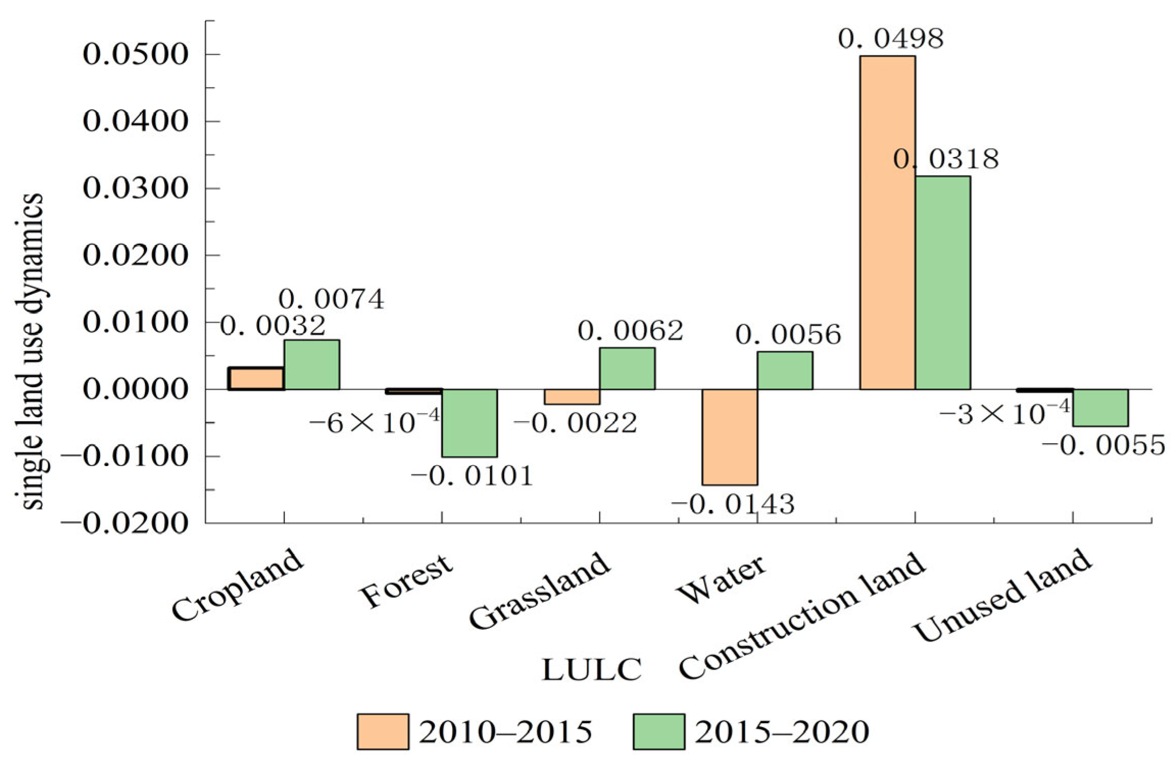
From 2010 to 2020, cropland area in TNUA showed consistent expansion, while construction land exhibited continuous growth. Grassland coverage demonstrated an initial decline followed by recovery, mirroring the trend observed in water body. In contrast, forest area experienced persistent reduction, and unused land underwent continual contraction. Temporally, the most substantial changes occurred during 2015–2020 for cropland, forest, grassland, and unused land, whereas water body and construction land showed peak change rates during 2010–2015.

(2)

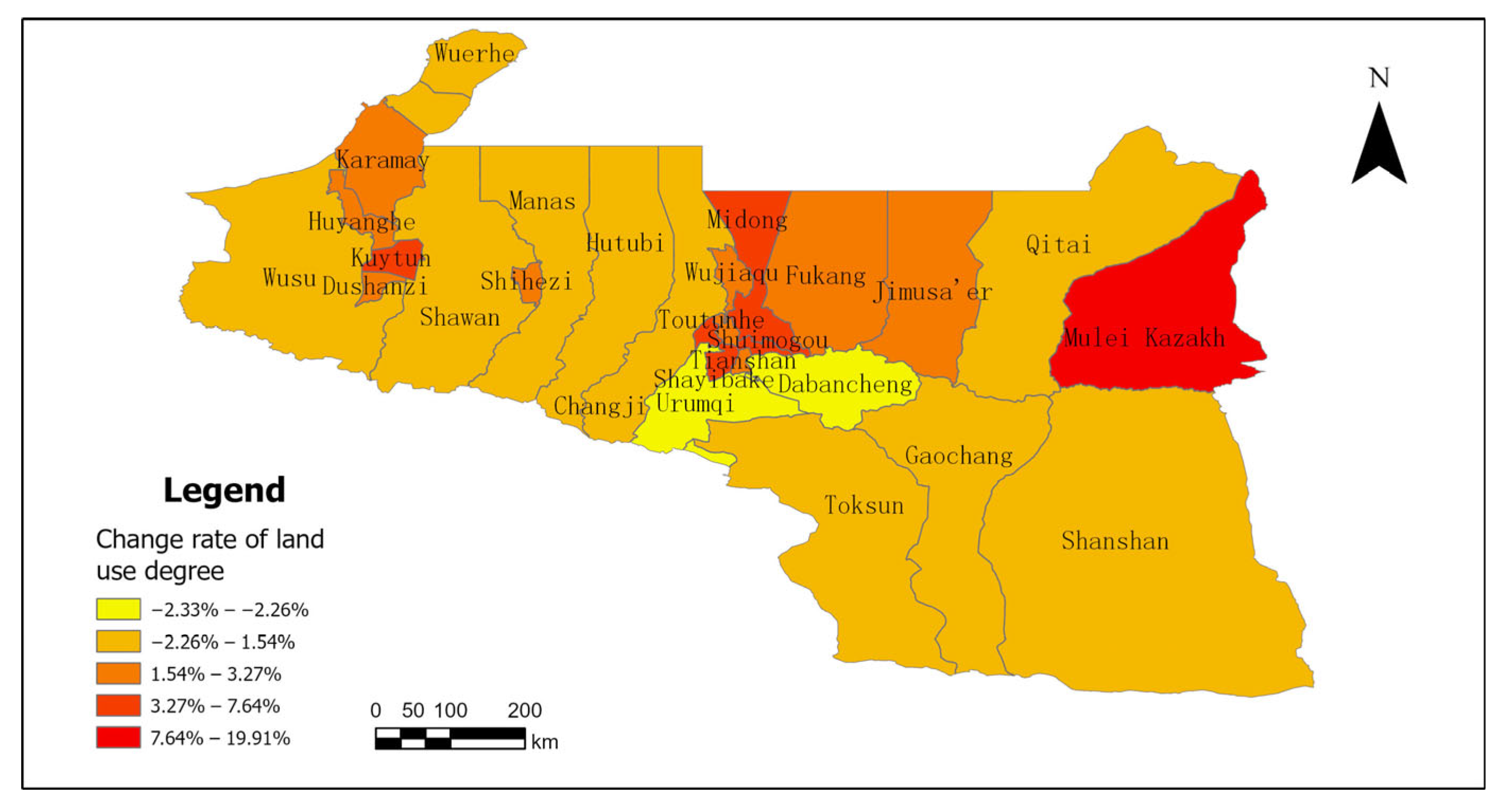
During the 2010–2020 period, the comprehensive land use intensity index in TNUA showed a significant increase from 157.8371 to 161.1008, demonstrating progressive intensification of anthropogenic land use activities and sustained regional development. Notably, the Shayibake District exhibited the most rapid intensification of land use among all study areas during this decade.

(3)

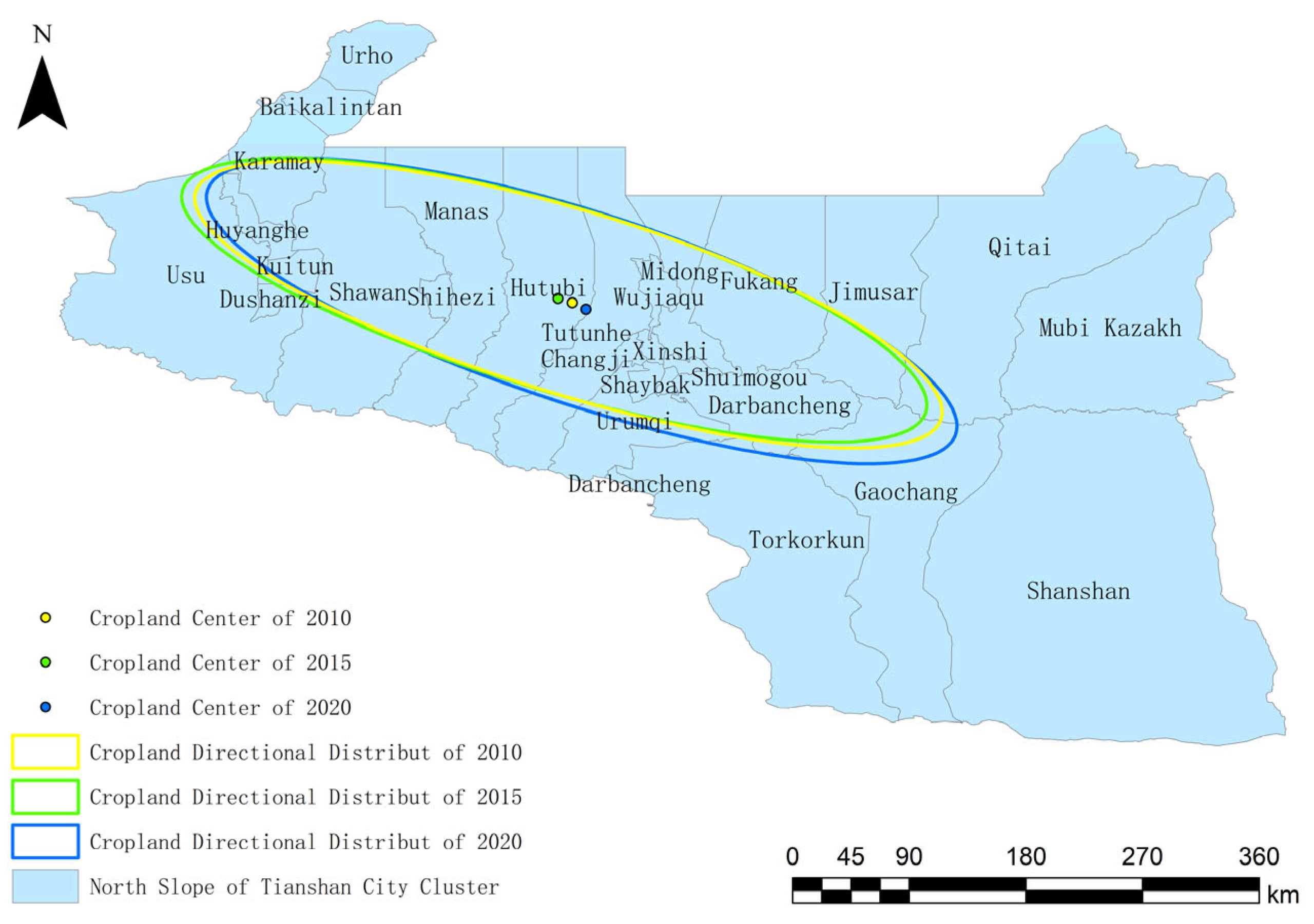
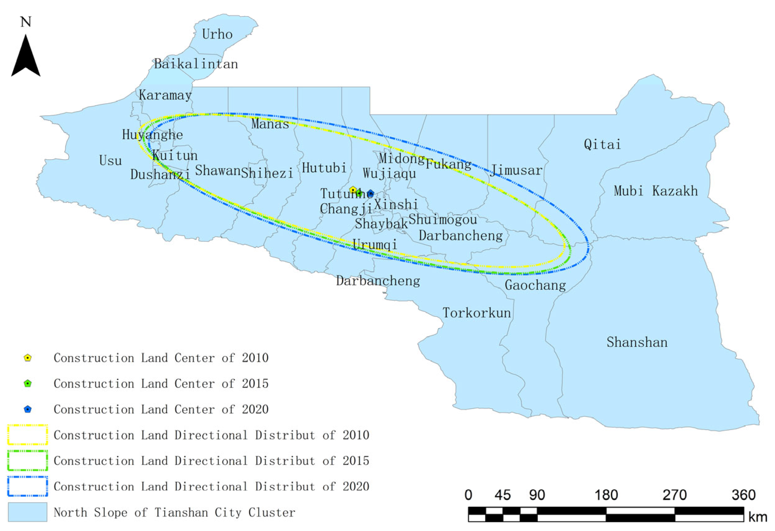
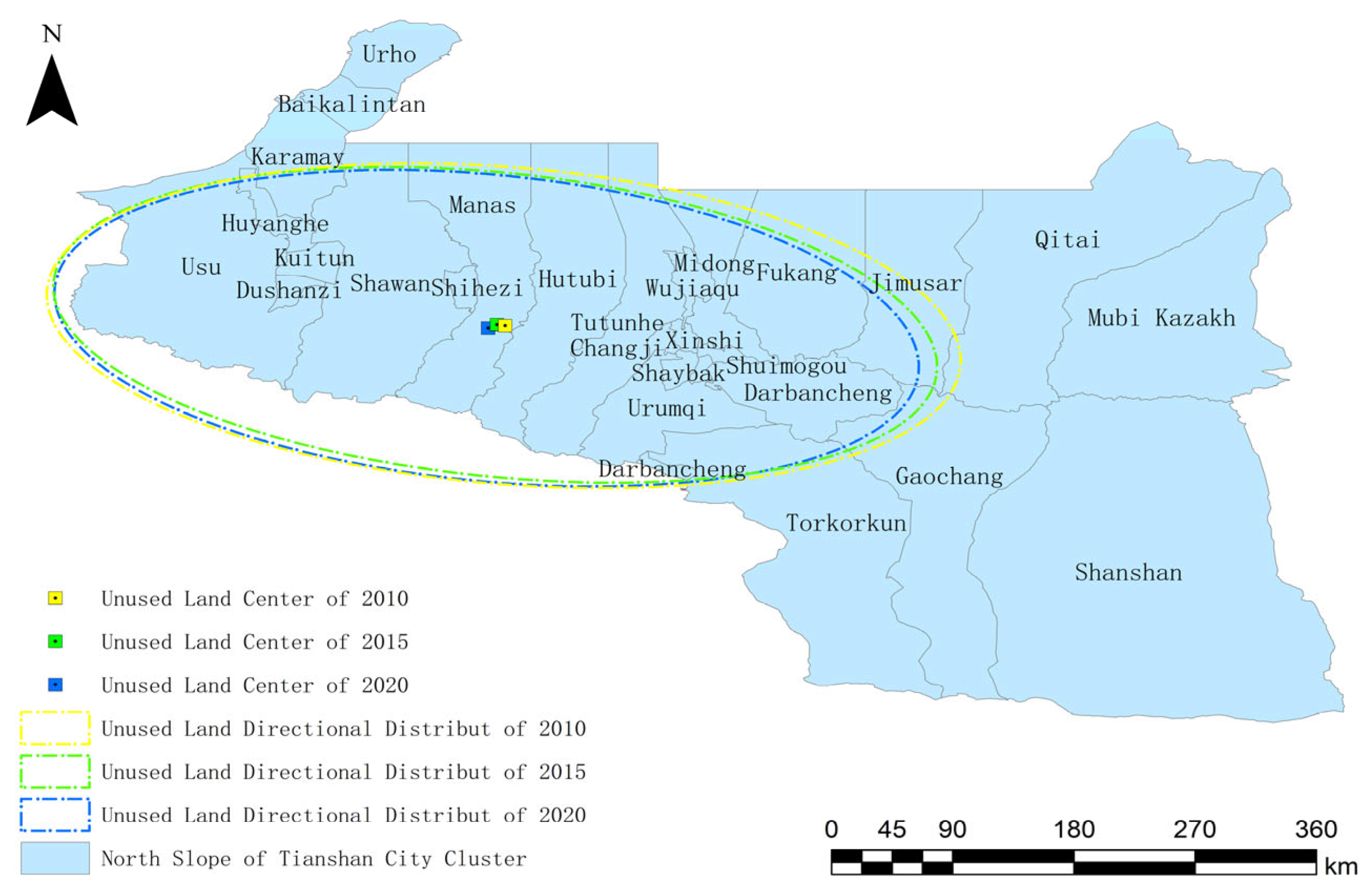
Analysis of centroid migration patterns revealed two key spatial relationships: (a) cropland displacement vectors showed strong correspondence with water body movements, reflecting the coupled development of agriculture and water resources in northern Tianshan’s oasis ecosystems; (b) construction land centroid trajectories displayed inverse directional trends relative to unused land, demonstrating urbanization-driven land conversion processes with a distinct eastward shift in urban expansion focus.

(4)

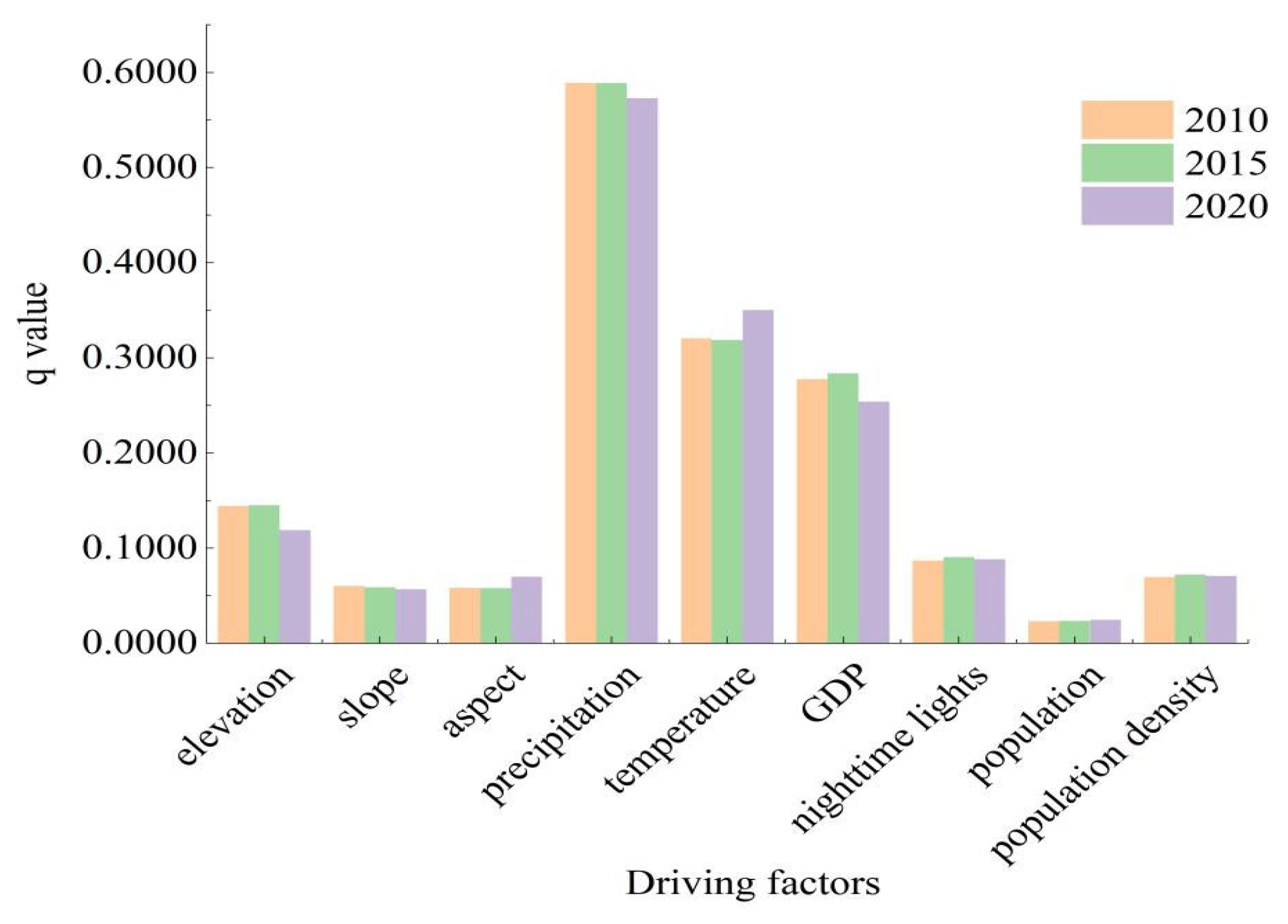
The driving factors showed varying influences across 2010, 2015 and 2020. Temperature, precipitation, GDP and elevation consistently remained the dominant factors affecting land use changes. Interaction analysis revealed that all factor interactions exhibited either two-factor enhancement or nonlinear enhancement effects, with neither independent nor weakening effects observed. This demonstrates that combined factors have greater explanatory power than individual factors alone.

(5)

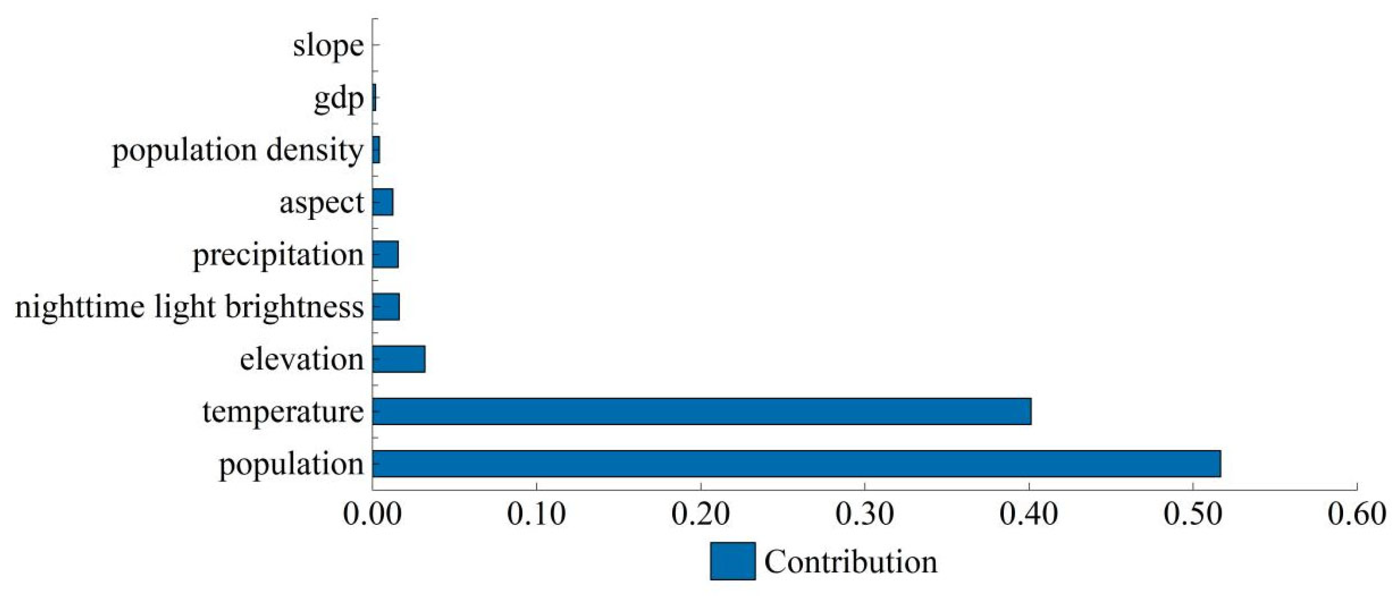
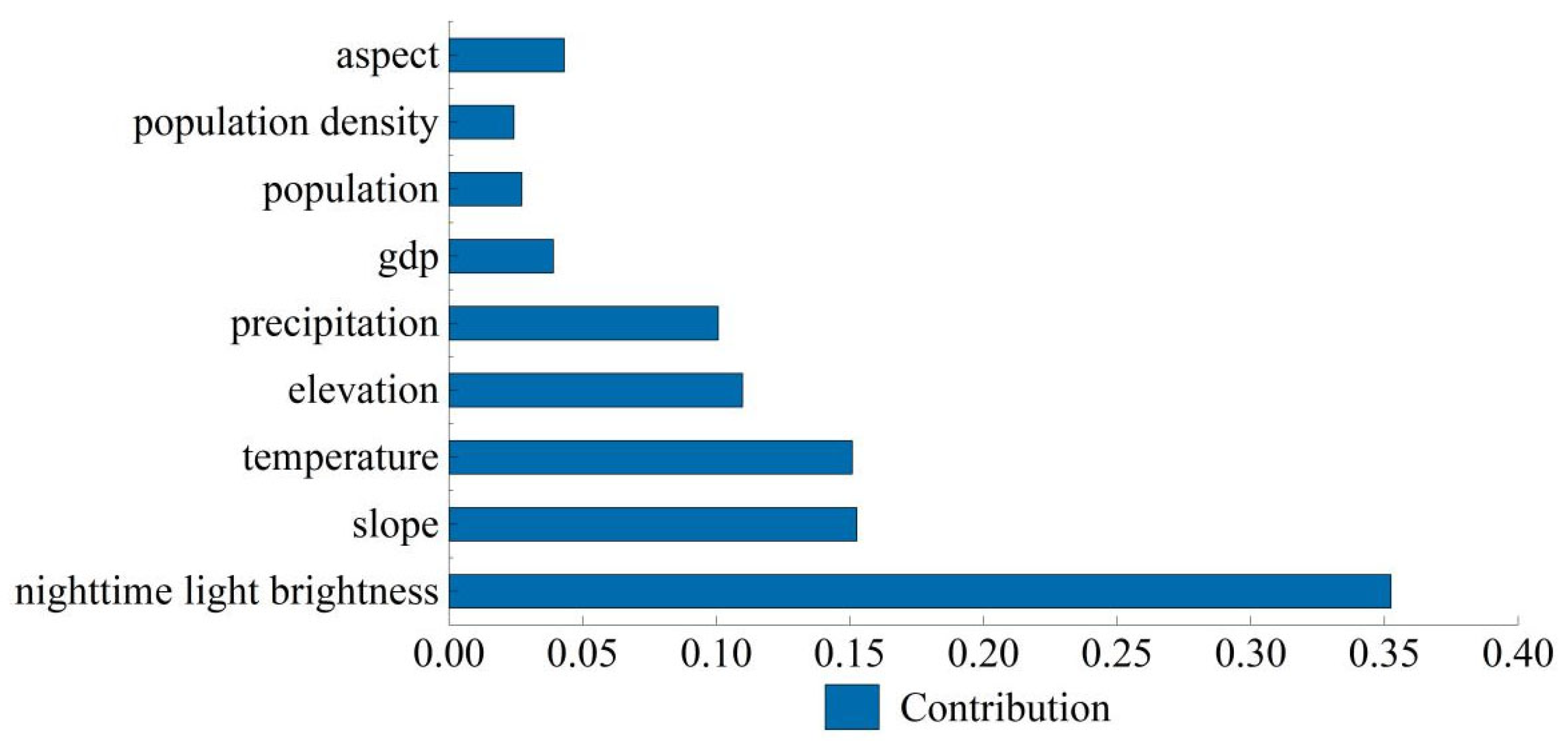
Distinct sets of driving factors were identified for different land use expansions. Water body expansion showed strong associations with population density, air temperature, and elevation. Cropland expansion was principally governed by slope, elevation, nighttime light brightness, and population density. For construction land expansion, the key determinants were nighttime light, slope, and air temperature.

(6)

The PLUS model exhibited high predictive accuracy for simulating land use changes. Projection results indicate consistent annual declines in unused land and forest area during 2025–2035, contrasting with progressive expansion of cropland, grassland, water body, and construction land throughout the projection period.

References

1. Chen, M.; Xian, Y.; Wang, P.; Ding, Z. Climate change and multi-dimensional sustainable urbanization. J. Geogr. Sci. 2021, 31, 1328–1348. [Google Scholar] [CrossRef]
2. Fang, C.; Gao, Q.; Zhang, X.; Cheng, W. Spatiotemporal characteristics of the expansion of an urban agglomeration and its effect on the eco-environment: Case study on the northern slope of the Tianshan Mountains. Sci. China Earth Sci. 2019, 62, 1461–1472. [Google Scholar] [CrossRef]
3. Ellis, E.C. Land use and ecological change: A 12,000-year history. Annu. Rev. Environ. Resour. 2021, 46, 1–33. [Google Scholar] [CrossRef]
4. Nebie, E.K.; West, C.T. Migration and land-use and land-cover change in Burkina Faso: A comparative case study. J. Polit. Ecol. 2019, 26, 614–632. [Google Scholar]
5. Msofe, N.K.; Sheng, L.; Lyimo, J. Land use change trends and their driving forces in the Kilombero Valley Floodplain, Southeastern Tanzania. Sustainability 2019, 11, 505. [Google Scholar] [CrossRef]
6. Chisanga, C.B.; Phiri, D.; Mubanga, K.H. Multi-decade land cover/land use dynamics and future predictions for Zambia: 2000–2030. Discov. Environ. 2024, 2, 38. [Google Scholar] [CrossRef]
7. Lambin, E.F.; Turner, B.L.; Geist, H.J.; Agbola, S.B.; Angelsen, A.; Bruce, J.W.; Coomes, O.T.; Dirzo, R.; Fischer, G.; Folke, C.; et al. The causes of land-use and land-cover change: Moving beyond the myths. Glob. Environ. Change 2001, 11, 261–269. [Google Scholar] [CrossRef]
8. Allan, A.; Soltani, A.; Abdi, M.H.; Zarei, M. Driving forces behind land use and land cover change: A systematic and bibliometric review. Land 2022, 11, 1222. [Google Scholar] [CrossRef]
9. Wu, H.; Lin, A.; Xing, X.; Song, D.; Li, Y. Identifying core driving factors of urban land use change from global land cover products and POI data using the random forest method. Int. J. Appl. Earth Obs. Geoinf. 2021, 103, 102475. [Google Scholar] [CrossRef]
10. Peng, K.; Jiang, W.; Ling, Z.; Hou, P.; Deng, Y. Evaluating the potential impacts of land use changes on ecosystem service value under multiple scenarios in support of SDG reporting: A case study of the Wuhan urban agglomeration. J. Clean. Prod. 2021, 307, 127321. [Google Scholar] [CrossRef]
11. Zhang, P.; Liu, L.; Yang, L.; Zhao, J.; Li, Y.; Qi, Y.; Ma, X.; Cao, L. Exploring the response of ecosystem service value to land use changes under multiple scenarios coupling a mixed-cell cellular automata model and system dynamics model in Xi’an, China. Ecol. Indic. 2023, 147, 110009. [Google Scholar] [CrossRef]
12. Pijanowski, B.C.; Brown, D.G.; Shellito, B.A.; Manik, G.A. Using neural networks and GIS to forecast land use changes: A land transformation model. Comput. Environ. Urban Syst. 2002, 26, 553–575. [Google Scholar] [CrossRef]
13. Gharaibeh, A.; Shaamala, A.; Obeidat, R.; Al-Kofahi, S. Improving land-use change modeling by integrating ANN with Cellular Automata-Markov Chain model. Heliyon 2020, 6, e04824. [Google Scholar] [CrossRef]
14. Doelman, J.C.; Stehfest, E.; Tabeau, A.; van Meijl, H.; Lassaletta, L.; Gernaat, D.E.; Hermans, K.; Harmsen, M.; Daioglou, V.; Biemans, H.; et al. Exploring SSP land-use dynamics using the IMAGE model: Regional and gridded scenarios of land-use change and land-based climate change mitigation. Glob. Environ. Change 2018, 48, 119–135. [Google Scholar] [CrossRef]
15. Leta, M.K.; Demissie, T.A.; Tränckner, J. Modeling and prediction of land use land cover change dynamics based on land change modeler (LCM) in Nashe watershed, upper Blue Nile basin, Ethiopia. Sustainability 2021, 13, 3740. [Google Scholar] [CrossRef]
16. Koko, A.F.; Han, Z.; Wu, Y.; Abubakar, G.A.; Bello, M. Spatiotemporal land use/land cover mapping and prediction based on hybrid modeling approach: A case study of Kano Metropolis, Nigeria (2020–2050). Remote Sens. 2022, 14, 6083. [Google Scholar] [CrossRef]
17. Avtar, R.; Rinamalo, A.V.; Umarhadi, D.A.; Gupta, A.; Khedher, K.M.; Yunus, A.P.; Singh, B.P.; Kumar, P.; Sahu, N.; Sakti, A.D. Land use change and prediction for valuating carbon sequestration in Viti Levu island, Fiji. Land 2022, 11, 1274. [Google Scholar] [CrossRef]
18. Liang, X.; Guan, Q.; Clarke, K.C.; Liu, S.; Wang, B.; Yao, Y. Understanding the drivers of sustainable land expansion using a patch-generating land use simulation (PLUS) model: A case study in Wuhan, China. Comput. Environ. Urban Syst. 2021, 85, 101569. [Google Scholar] [CrossRef]
19. National Development and Reform Commission Office. Notice on Accelerating the Compilation of Urban Agglomeration Planning; National Development and Reform Commission: Beijing, China, 2016. [Google Scholar]
20. GS(2020)4619; Standard Map of China. Ministry of Natural Resources of the People’s Republic of China: Beijing, China, 2020.
21. Li, X.; Zhou, Y.; Zhao, M.; Zhao, X. A harmonized global nighttime light dataset 1992–2018. Sci. Data 2020, 7, 168. [Google Scholar] [CrossRef]
22. Wang, J.F.; Xu, C.D. Geodetector: Principle and prospective. Acta Geogr. Sin. 2017, 72, 116–134. [Google Scholar]
23. Zhuang, D.; Liu, J. Study on the model of regional differentiation of land use degree in China. J. Nat. Resour. 1997, 12, 105–111. [Google Scholar]
24. Department of Natural Resources of Xinjiang Uygur Autonomous Region. The 14th Five-Year Plan for the Protection and Development of Land Resources in Xinjiang Uygur Autonomous Region; Department of Natural Resources of Xinjiang Uygur Autonomous Region: Urumqi, China, 2021. [Google Scholar]
25. Department of Natural Resources of Xinjiang Uygur Autonomous Region. Revised and Simplified Version of the General Land Use Plan of Xinjiang Uygur Autonomous Region (2006–2020); Department of Natural Resources of Xinjiang Uygur Autonomous Region: Urumqi, China, 2018. [Google Scholar]
26. Li, X.; Qin, D.; He, X.; Wang, C.; Yang, G.; Li, P.; Liu, B.; Gong, P.; Yang, Y. Spatial and temporal changes in land use and landscape pattern evolution in the economic belt of the Northern Slope of the Tianshan Mountains in China. Sustainability 2024, 16, 7003. [Google Scholar] [CrossRef]
27. Department of Ecology and Environment of Xinjiang Uygur Autonomous Region. The 14th Five-Year Plan for Ecological Environmental Protection in Xinjiang; Department of Ecology and Environment of Xinjiang Uygur Autonomous Region: Urumqi, China, 2022. [Google Scholar]
28. Zhao, Y.; Kasimu, A.; Gao, P.; Liang, H. Spatiotemporal changes in the urban landscape pattern and driving forces of LUCC characteristics in the urban agglomeration on the Northern Slope of the Tianshan Mountains from 1995 to 2018. Land 2022, 11, 1745. [Google Scholar] [CrossRef]
29. Shahbazian, Z.; Faramarzi, M.; Rostami, N.; Mahdizadeh, H. Integrating logistic regression and cellular automata–Markov models with the experts’ perceptions for detecting and simulating land use changes and their driving forces. Environ. Monit. Assess. 2019, 191, 422. [Google Scholar] [CrossRef]
30. Buya, S.; Tongkumchum, P.; Owusu, B.E. Modelling of land-use change in Thailand using binary logistic regression and multinomial logistic regression. Arab. J. Geosci. 2020, 13, 437. [Google Scholar] [CrossRef]
31. Braimoh, A.K.; Onishi, T. Spatial determinants of urban land use change in Lagos, Nigeria. Land Use Policy 2007, 24, 502–515. [Google Scholar] [CrossRef]
32. Zhang, J.; Liu, Z.; Li, S. Research on land use simulation of incorporating historical information into the FLUS model—Setting Songyuan City as an example. Sustainability 2022, 14, 3828. [Google Scholar] [CrossRef]
33. Wang, Y.; Shen, J.; Yan, W.; Chen, C. Backcasting approach with multi-scenario simulation for assessing effects of land use policy using GeoSOS-FLUS software. MethodsX 2019, 6, 1384–1397. [Google Scholar] [CrossRef]
34. Liu, P.; Hu, Y.; Jia, W. Land use optimization research based on FLUS model and ecosystem services–setting Jinan City as an example. Urban Clim. 2021, 40, 100984. [Google Scholar] [CrossRef]
35. Li, D.; Chang, Y.; Simayi, Z.; Yang, S. Multi-scenario dynamic simulation of urban agglomeration development on the northern slope of the Tianshan Mountains in Xinjiang, China, with the goal of high-quality urban construction. Sustainability 2022, 14, 6862. [Google Scholar] [CrossRef]
Figure 1. Map of TNUA administrative divisions. Note: The map is based on the standard map with review number GS(2020)4619 [20], downloaded from the standard map service website of the State Administration of Surveying, Mapping, and Geoinformation. The boundary of the base map is not modified.
Land 14 01123 g001
Figure 2. Change of average annual rate of change attitude in TNUA from 2010 to 2020.
Land 14 01123 g002
Figure 3. Change rate of land use degree in TNUA.
Land 14 01123 g003
Figure 4. Center of gravity transfer of cropland from 2010 to 2020.
Land 14 01123 g004
Figure 5. Center of gravity transfer water body from 2010 to 2020.
Land 14 01123 g005
Figure 6. Center of gravity transfer of construction land from 2010 to 2020.
Land 14 01123 g006
Figure 7. Center of gravity transfer of unused land from 2010 to 2020.
Land 14 01123 g007
Figure 8. Factor detection results.
Land 14 01123 g008
Figure 9. Factor interaction heat map.
Land 14 01123 g009
Figure 10. Contribution of drivers to water body expansion.
Land 14 01123 g010
Figure 11. Contribution of drivers to cropland expansion.
Land 14 01123 g011
Figure 12. Contribution of drivers to construction land expansion.
Land 14 01123 g012
Figure 13. Projected land use types for 2025.
Land 14 01123 g013
Figure 14. Projected land use types for 2030.
Land 14 01123 g014
Figure 15. Projected land use types for 2035.
Land 14 01123 g015
Figure 16. Changes in the corresponding area of each land use type over the years.
Land 14 01123 g016