1. Introduction
Transit-oriented development is an urban planning strategy addressing the challenges of densely populated cities by enhancing accessibility to public transportation. This strategy aims to foster a sustainable transportation system by reducing reliance on private vehicles and encouraging walking, cycling, and public transit [
1]. However, the pervasive spread of coronavirus disease 2019 (COVID-19) posed significant risks to these systems. In response, governments worldwide implemented movement restrictions and social distancing measures, which, in turn, led to a significant decrease in mobility [
2,
3,
4]. Notably, during the COVID-19 pandemic, the decline in public transportation use was more pronounced than personal vehicle use [
5,
6,
7].
Numerous studies have investigated the changes in the relationship between public transportation usage patterns and the built environment due to COVID-19 [
6,
8,
9]. However, these studies often lack a spatial analysis or the ability to visualize the spatial discrepancies in usage. Moreover, while they focused on overall trends, they did not adequately capture how the relationships between key factors, such as demographic variables and land use, shifted regionally in the post-pandemic context. This research differs by employing advanced spatial models, specifically multiscale geographically weighted regression (MGWR) and geographical random forest (GRF), to not only capture the changing relationships between public transport usage and influencing factors but also to account for spatial heterogeneity in these relationships. Unlike traditional approaches, this study integrates spatial bandwidth information from GWR into GRF, offering deeper insights into local dependencies and allowing for the identification of region-specific transit demand drivers. This method provides a more nuanced understanding of transit patterns, especially for vulnerable groups, making it a more effective tool for targeted transit planning in the post-pandemic era. By doing so, this study contributes to the existing literature by offering a more comprehensive, spatially aware framework for addressing public transit challenges in a post-COVID-19 world.
To achieve this, the study sets out three specific objectives: (1) to spatially identify changes in bus ridership patterns between pre- and post-pandemic periods, (2) to compare and evaluate the explanatory power of GWR and MGWR in capturing regional variations, and (3) to determine the most influential factors using RF and GRF models, incorporating spatial dependency through the GRF approach. These steps aim to support evidence-based and regionally adaptive public transportation strategies in the wake of COVID-19.
3. Data and Methodology
3.1. Study Area and Research Flow
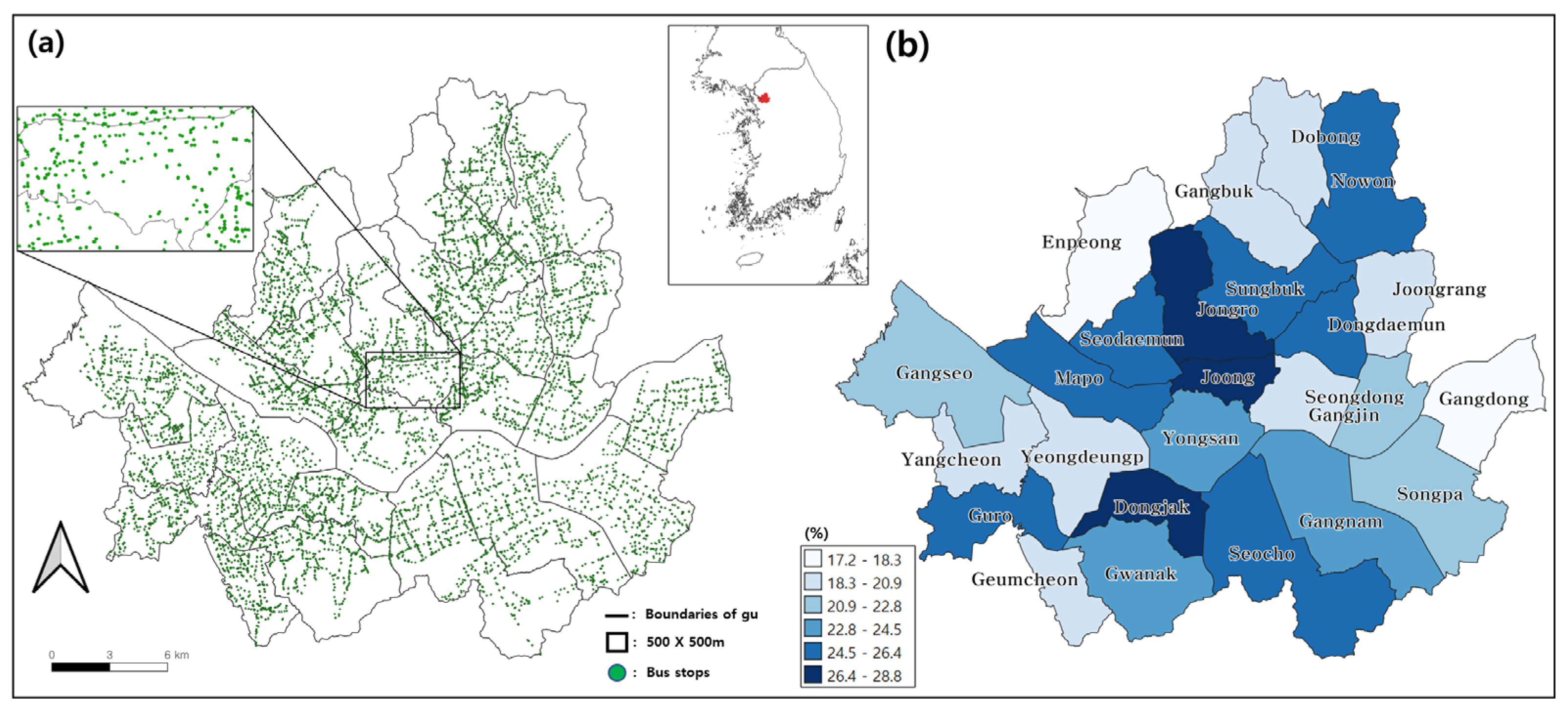
The research area on the map in
Figure 1a is Seoul, the capital of the Republic of Korea, with 9.39 million residents as of 2023.
At the center of the Korean Peninsula in East Asia, Seoul is the largest city in the Republic of Korea. Due to its complex urban structure and substantial population, Seoul exhibits considerable intra-city variation, with distinct demographic, land-use, and mobility patterns across different districts. In 2021, Seoul had the highest percentage of confirmed COVID-19 cases in the Republic of Korea, accounting for approximately 53.5% of the total population. This led to the implementation of strict social distancing measures, which resulted in a significant reduction in movement, particularly in public transportation. The map in
Figure 1b depicts a notable decrease in bus usage across most areas of Seoul. The left panel in
Figure 1a presents the distribution of bus stops in the city, and the following diagram outlines the overall research framework. Given its urban complexity, high dependency on public transit, and diverse spatial characteristics, Seoul provides a suitable and representative case for studying the spatial impacts of COVID-19 on transit usage.
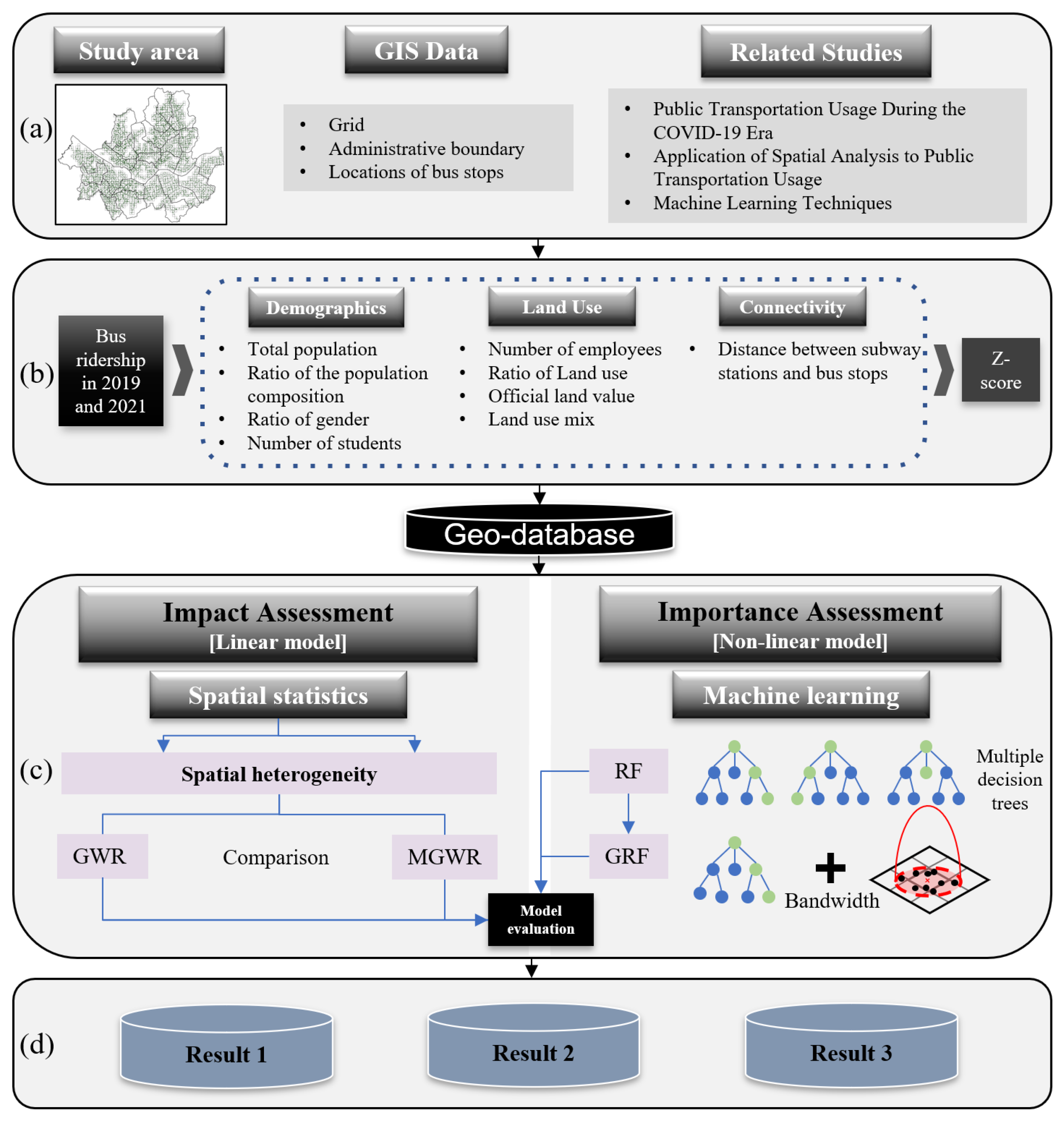
First, in the initial stage (
Figure 2a), geographical information system (GIS) shapefiles based on a grid (500 m × 500 m) were employed to examine the spatial changes in public transportation volume in Seoul. A map was created to display the bus stops, with the daily average number of boarding and alighting passengers at each bus stop serving as the dependent variable. Relevant studies were reviewed to identify factors affecting changes in public transportation volume using a linear analysis.
In the second stage (
Figure 2b), variables directly affecting bus usage were identified. An analysis of the connectivity between public transportation modes, such as buses and subways, was conducted. The collected data on these factors were standardized to mitigate scale disparities caused by heterogeneous data types, ensuring that specific factors did not disproportionately influence the results. Subsequently, a geodatabase for the research analysis was established.
In the third stage (
Figure 2c), an influence analysis and importance assessment were performed to observe the spatial changes in public transportation volume. First, an analysis was conducted to understand how bus usage spatially depends on and varies with the selected factors in this study. Next, a GWR model was applied to analyze which variables had a more significant spatial influence. As mentioned, this study compared GWR and MGWR methods to determine the most suitable approach for the research objectives. Finally, an RF machine learning technique and GRF model incorporating bandwidth concepts were used for importance assessment to analyze and identify significant factors by region (
Figure 2c).
3.2. Data Collection
The dependent variable, the daily average number of bus rides, was derived from smart card transportation data provided by Seoul’s public bus operators.
The data are from 2019 (before the COVID-19 pandemic) and 2021 (when social distancing policies were most strictly enforced throughout the year). Data from 2022 and 2023 were omitted as these years represented a transitional phase characterized by the gradual relaxation of restrictions and shifting travel behaviors, which could introduce confounding effects into the assessment of the pandemic’s impact.
Explanatory variables affecting bus usage were chosen based on previous studies exploring the relationship between public transportation and diverse factors [
6,
13,
15,
17,
21,
22]. These variables are categorized into demographics, land-use characteristics, and connectivity.
Socioeconomic data were sourced from grid-cell-based datasets published by Korea’s National Geographic Information Institute. Grid-based data are used because continuous spatial phenomena can be grasped in detail compared to existing traffic analysis zones and the bias of spatial analysis models is improved according to the size of spatial units in urban and non-urban cities. While alternatives such as Transport Analysis Zones offer population-balanced spatial units, the grid-based approach was preferred for its compatibility with high-resolution spatial datasets.
Additionally, the smart card data, which are originally recorded at the level of individual bus stops, were spatially aggregated to match the grid cells using the geographic coordinates of each stop. This process ensured compatibility with other grid-based datasets used in the study. However, one notable limitation of the smart card dataset is the incomplete recording of alighting information, particularly for bus users, which may affect the spatial precision of the dependent variable. In such cases, approximations or partial records may have been used, potentially introducing spatial uncertainty.
Despite offering fine spatial granularity, the grid-based approach may also result in inhomogeneous population or land-use distributions within cells, especially in dense metropolitan areas like Seoul. For instance, grids in central business districts may contain significantly higher population density and functional diversity compared to suburban grids. During the COVID-19 pandemic, strict social distancing measures led to reduced usage of commercial facilities and a shift in population activity patterns, with more movements concentrated around residential areas. These behavioral changes may have indirectly influenced several variables, including population density, land-use complexity, and public transit demand. These limitations and contextual factors should be taken into account when interpreting the findings.
Among the various variables, land-use complexity represents the number of different building use types within each grid cell. This metric was calculated by counting the types of buildings present based on 28 building use categories defined in the Building Act and its Enforcement Decree. These include residential, commercial, religious, cultural, medical, educational, industrial, and recreational uses, among others. A higher number of distinct building uses in a grid reflects a higher level of land-use complexity. Unlike more nuanced indices such as the Shannon Diversity Index, this approach provides a straightforward measure of use diversity, though it does not reflect the balance or evenness of land-use distribution. Spatial adjustments were applied to align bus usage data and subway station proximity data with these grid cells. The distance to subway stations represents the mean Euclidean distance from each grid centroid to the closest subway station, capturing multimodal accessibility. Classical graph-theoretic measures were considered but not applied due to data limitations and the focus on direct physical proximity. Bus usage was aggregated to match the grid boundaries.
Table 1 lists the definitions of 12 independent variables across these categories, and
Table 2 provides descriptive statistics for the determinants in this study. Factors without values for 2019 used the most recent available data because data for both 2019 and 2021 were not available simultaneously. All explanatory variables were standardized using Z-score normalization to ensure comparability and prevent scale bias prior to performing the analysis.
In
Table 2, the changes experienced by the variables between 2019 and 2021 are indicative of the influence of the COVID-19 pandemic and related social distancing policies. For example, bus usage decreased from an average of 944 rides in 2019 to 717 in 2021, reflecting reduced public transportation demand due to pandemic restrictions. Demographic variables such as the aging population ratio also saw changes, with an increase in the proportion of elderly individuals in 2021, possibly due to restrictions affecting younger populations more significantly. Moreover, land-use characteristics show a clear impact of pandemic policies: commercial area usage declined as businesses faced restrictions, while residential areas saw an increase, possibly reflecting people spending more time at home during lockdowns. These shifts in land-use complexity and other variables reflect broader shifts in behavior and land-use patterns due to the pandemic.
3.3. Methods
The GWR and MGWR methods were employed to analyze how the local relationship between bus usage and influencing factors changes. Brunsdon et al. introduced GWR, a local regression model that estimates relationships based on the values of the dependent and explanatory variables at each location [
30]. Unlike traditional global regression methods that assume a constant relationship between variables across space, GWR allows spatially varying the parameters [
31]. The formulation of GWR is as follows:
In Equation (1),
represents the dependent variable for the
th grid,
denotes the coefficient for the
th grid,
denotes the
th explanatory variable for the
th grid, and
indicates the error term [
14].
The GWR estimation process involves setting a bandwidth around a location
and calculating the weights for each observation based on the distance from the centroid. The model coefficients are estimated using the weighted least squares method [
30]. In this study, the GWR model employs the bi-square distance weighting method, where weights decrease with distance and become zero beyond a certain threshold. Despite using grid units with a constant spatial distribution, this study applies an adaptive kernel method to exclude grids without bus stops or population segments.
To standardize the data before applying the GWR and MGWR models, the explanatory variables were normalized using Z-scores. This ensures that all variables are on the same scale and comparable, mitigating any potential bias introduced by differences in units or magnitude.
Bandwidths were selected using the golden division method, applying the golden ratio to determine optimal values. The optimal bandwidth was chosen based on the smallest Akaike’s information criterion with a small-sample correction (
AICc) value [
34,
36]. AICc was chosen because it balances model fit and complexity, penalizing models with too many parameters, which helps prevent overfitting in the context of the spatial data.
The limitations of GWR noted in previous research are addressed by employing MGWR, allowing for varying spatial scales in the relationship between the dependent and explanatory variables. Fotheringham et al. proposed MGWR, which estimates local parameters by adjusting bandwidths according to the spatial characteristics of explanatory variables [
31,
46]. The formulation of MGWR is as follows:
In Equation (2),
represents the bandwidth for calibrating the
th conditional relationship [
14]. This study employs MGWR to capture the local influences of factors more effectively on bus usage than GWR. Geographically weighted regression (GWR) and multiscale geographically weighted regression (MGWR) analyses were performed using the MGWR 2.0 software package, a Python-based tool developed by researchers at the University of Arizona. Next, RF and GRF were applied to assess the local importance of each factor affecting bus usage. Breiman introduced RF, an ensemble method comprising multiple decision trees that aggregate results via majority voting based on random inputs [
42,
47]. The RF method determines factor importance by modeling nonlinear relationships between dependent and explanatory variables. This method constructs numerous decision trees in parallel using bootstrap aggregating (bagging), reducing the variance and enhancing model stability, mitigating overfitting and noise sensitivity in individual trees [
21]. Each decision tree is trained on two-thirds of the data, whereas the remaining third, known as the out-of-bag set, is used to estimate model performance. The out-of-bag method eliminates the need for separate cross-validation or testing sets. Final predictions were averaged across all decision trees to produce the overall RF output [
45,
48]. To select the optimal parameters for the RF model, we employed a random grid search method using the H
2O package in R 4.2.0, which automates the search for the best hyperparameters by testing different combinations.
Noted for its simplicity, RF is versatile in addressing various predictive problems and can handle large datasets [
49]. Moreover, RF mitigates the risk of overfitting due to its method of training multiple decision trees on varied datasets [
20]. This characteristic makes RF a robust classifier that is effective when working with large datasets and appropriately tuned hyperparameters [
50]. This study employs a random grid search method for parameter optimization in RF using the H
2O package in R, a prominent statistical programming language [
20,
51].
GRF extends the RF model by incorporating spatial heterogeneity, which is not explicitly accounted for in RF. GRF also integrates the bandwidth from GWR, allowing for the generation of localized submodels rather than relying on a single global model. The spatial bandwidth in GRF was optimized using functions in the SpecialML package in R. GRF uses the bandwidth information obtained from GWR to adjust the spatial scale of the local models, reflecting the varying spatial dependencies across different locations. This integration allows GRF to capture the local variations more effectively than traditional RF models. Georganos et al. proposed that GRF extends the RF model by incorporating spatial heterogeneity, which is not explicitly accounted for in RF [
19]. In addition, GRF evaluates the local significance of each factor by integrating the bandwidth from GWR, and it generates local submodels rather than relying on a single global model [
20]. The formulation of GRF is as follows:
In Equation (3),
represents the predicted value of the RF at position
, and
indicates the center coordinate of position
. Other submodels are created at each location
and reflect only its adjacent values [
20]. Similarly to GWR, GRF can determine the type of kernel, and the adaptive method GWR is used in this work. The same parameters are used as in the RF model, and the optimal bandwidth was selected using functions embedded in the SpecialML package of the R programming language, ensuring a tailored model that reflects local spatial dependencies.
4. Results
4.1. Spatially Evaluating Determinants Influencing Public Bus Usage
In this section, GWR was employed to analyze the spatial heterogeneity by locally estimating the effects of explanatory variables on bus usage. The MGWR method was employed to perform a spatial heterogeneity analysis based on the distinctive characteristics of each factor to address the limitations of GWR.
Table 3 presents the results of the GWR model for 2019 and 2021.
The comparative analysis of the results from 2019 and 2021 reveals shifts in the coefficients of several variables. The coefficient for the population number increased from −39.030 to 0.898, and the coefficient for the over-65 population ratio rose from −11.185 to 58.193, transitioning from negative to positive effects on bus usage. Conversely, the coefficient for the number of students shifted from 3.013 to −26.251, changing from a positive to a negative effect. These variations imply alterations in bus-usage patterns associated with COVID-19. However, the GWR results may be subject to over- or underestimation due to the uniform bandwidth across all variables [
31]. The MGWR method was employed to address this limitation, allowing for variable-specific bandwidths based on the distribution characteristics.
Table 4 presents the MGWR model results for 2019 and 2021.
The comparison of the results from 2019 and 2021 reveals that the over-65 population ratio consistently positively affected bus usage in both periods; however, its coefficient value declined from 31.30 in 2019 to 0.07 in 2021. Similarly, the number of students transitioned from having a positive effect (32.57) in 2019 to a negative effect (−19.20) in 2021, aligning with the findings of the GWR analysis. Furthermore, the positive influence of land-use complexity significantly increased, rising from 116.6 in 2019 to 503.9 in 2021. These findings diverge from those in previous GWR analyses.
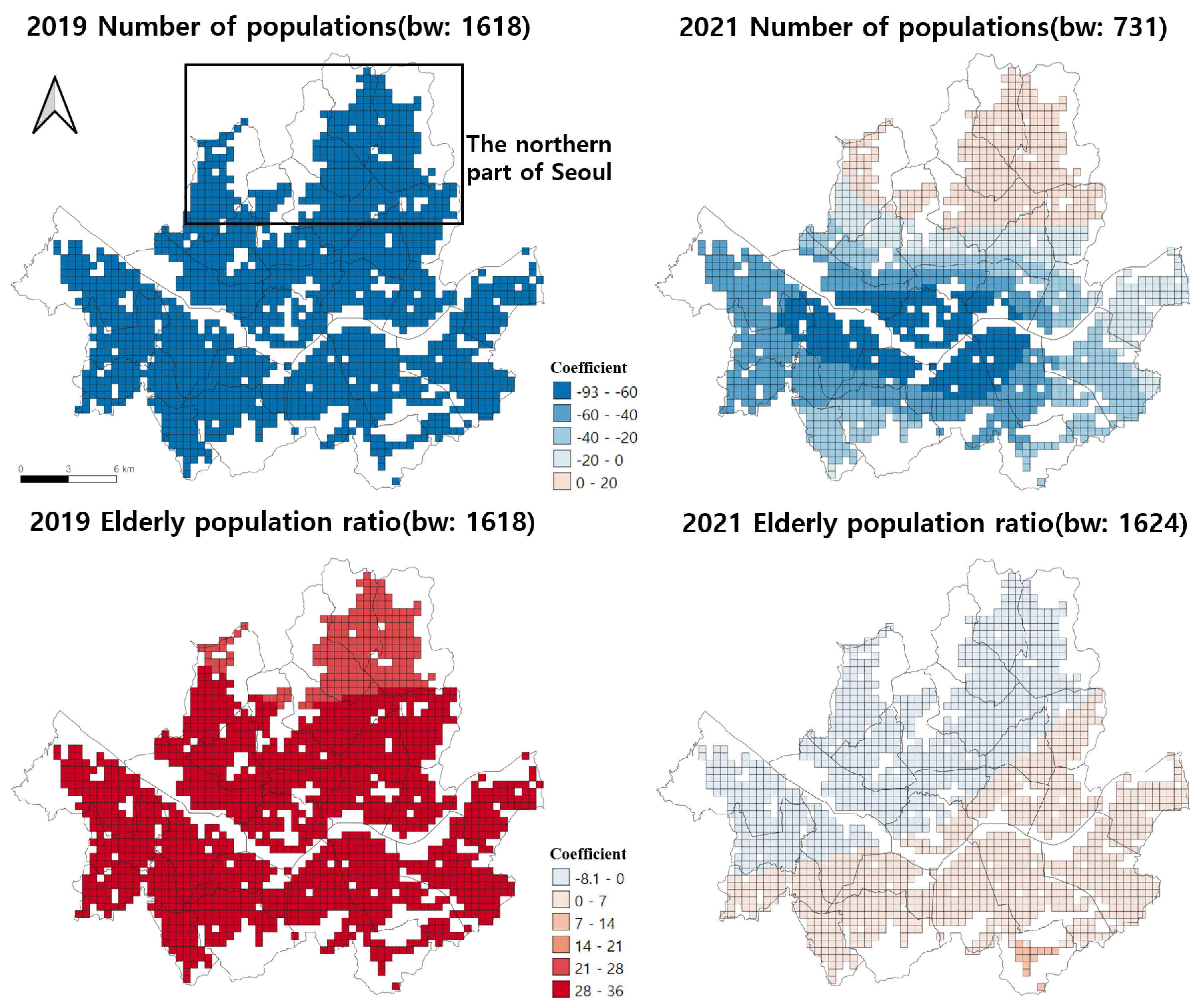
Figure 3 and
Figure 4 illustrate the local changes in these variables observed in the MGWR model. Four variables demonstrated notable changes: total population, over-65 population ratio, number of students, and land-use complexity.
As shown in
Figure 3, the total population variable exerted a negative influence on bus usage across most areas of Seoul in 2019. This may reflect a pre-pandemic urban environment where higher population areas, particularly in dense commercial or transit-rich zones, had more modal choices or greater reliance on subways or private transport. However, by 2021, this negative effect had diminished, particularly in central districts, and a positive relationship emerged in the northern parts of the city. This spatial shift suggests that population-driven demand for bus services increased in peripheral or residential areas during the pandemic recovery phase, potentially reflecting shifts in essential travel patterns, reduced subway usage due to infection concerns, or an increased reliance on local bus services in areas with limited alternative transit modes.
Conversely, the proportion of the over-65 population, which had a consistently positive impact on bus usage throughout Seoul in 2019, transitioned to a negative influence in 2021, especially in Gangseo-gu and the northern districts. This reversal may be associated with mobility restrictions among elderly populations due to health concerns, increased vulnerability to COVID-19, or changes in travel behavior such as reduced discretionary and non-essential trips. Additionally, service disruptions or perceived risks of crowded public spaces may have discouraged older residents from using buses.
The number of students exhibited the most pronounced change among the variables, positively affecting bus usage in 2019 across most regions, excluding parts of Guro-gu and Yangcheon-gu. However, by 2021, the number of students became a negative determinant in all regions. The change was attributed to remote education in middle and high schools due to COVID-19. Land-use complexity also underwent notable change: in 2019, it exhibited positive and negative effects depending on the region, but by 2021, it had a uniformly evenly weak positive effect across all areas. This is due to the simplification of people’s movement factors as a result of social distancing.
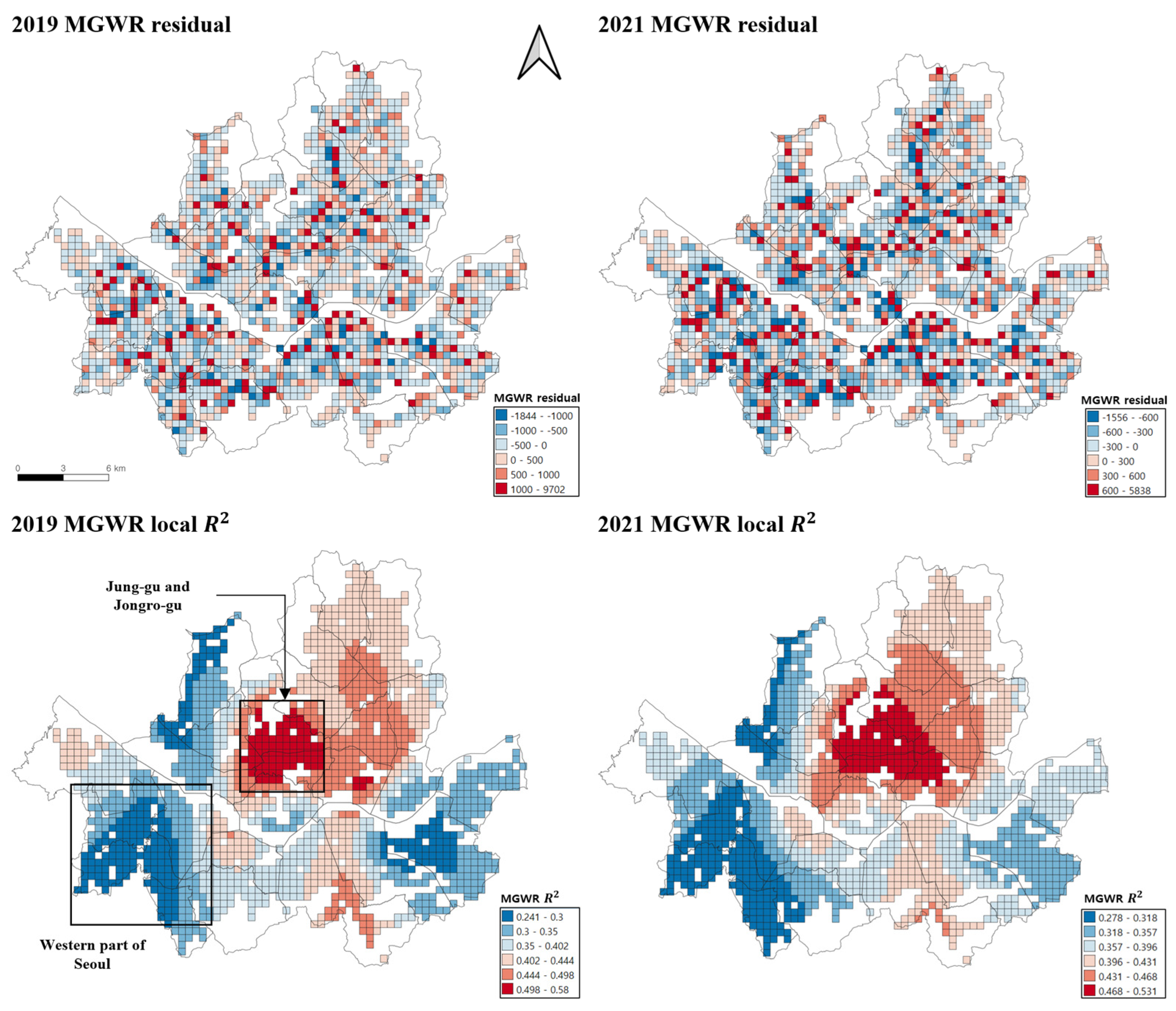
Figure 5 visualizes the residuals and
R-squared values from the MGWR model.
The two maps in
Figure 5 illustrate the spatial distribution of residuals, representing the difference between the actual and predicted values in the MGWR model. The map analysis indicates that the residuals from the MGWR model do not display any discernible spatial patterns. Moran’s
I values for the residuals in the 2019 and 2021 models were −0.016 and −0.018, respectively, suggesting a lack of significant spatial dependence in both models. At the bottom of
Figure 5, the two maps depict the spatial distribution of the local coefficients of determination for the MGWR model. The coefficient of determination exceeded 0.5 in Jung-gu and Jongno-gu, whereas it fell below 0.3 in western regions. These findings indicate that the effect of the determinants on bus usage varies across regions.
4.2. Ranking the Importance of Determinants
In previous analyses, spatial methods were employed based on linear relationships. This section applies nonparametric machine learning techniques, specifically RF and GRF, for further understanding. The RF analysis provided insight into the relative importance of each variable concerning bus usage. The GRF analysis offered a localized variable importance assessment, accounting for spatial correlations with neighboring regions.
Table 5 presents the results of the RF model for 2019 and 2021.
When comparing the results from the two periods, the importance ranking of certain variables shifted; however, no variable experienced a change in relative importance greater than 10. This finding indicates that the RF analysis, which does not account for spatial correlation between adjacent regions, insufficiently detected changes in bus-usage patterns attributable to COVID-19. A GRF analysis was conducted to address these limitations, incorporating the bandwidth concept from GWR.
Table 6 presents the results of the GRF models for 2019 and 2021.
Several notable changes in variable importance were observed when comparing the results from the two periods. Similarly to the RF model, the importance rankings of variables, such as the official land price and number of employees, shifted. In 2021, the relative importance of variables, such as the commercial area ratio, distance from subway stations, and productive population ratio, significantly increased, with changes exceeding 10. The over-65 population ratio (ranked 11th in 2019) advanced to sixth place in 2021, indicating the most substantial change.
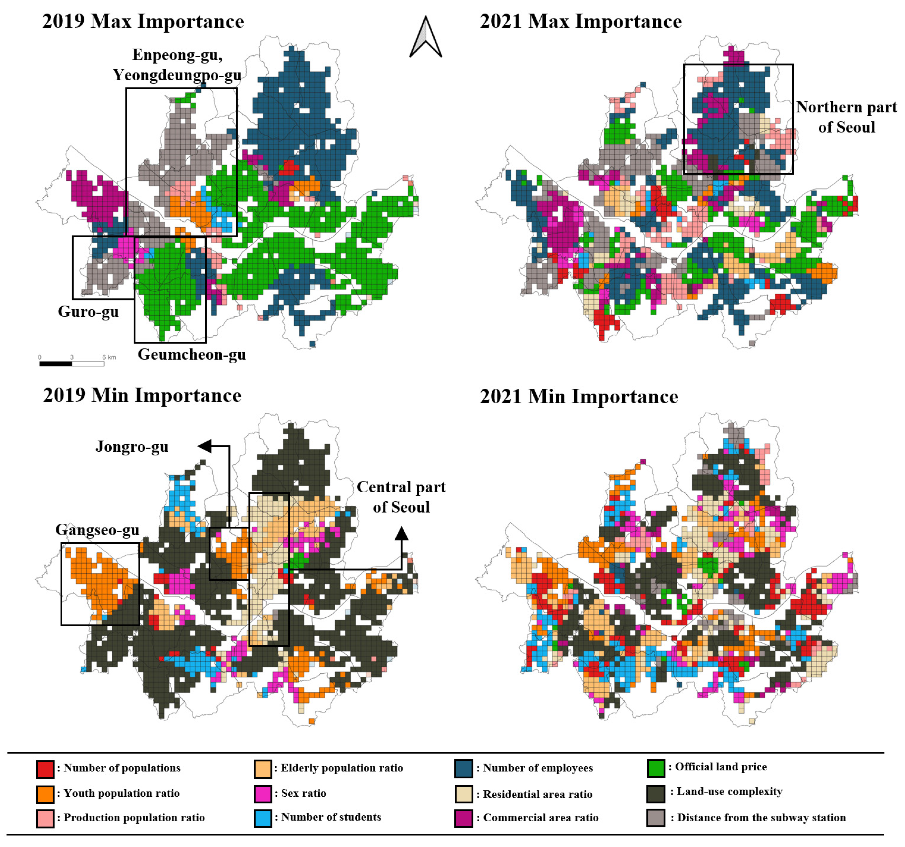
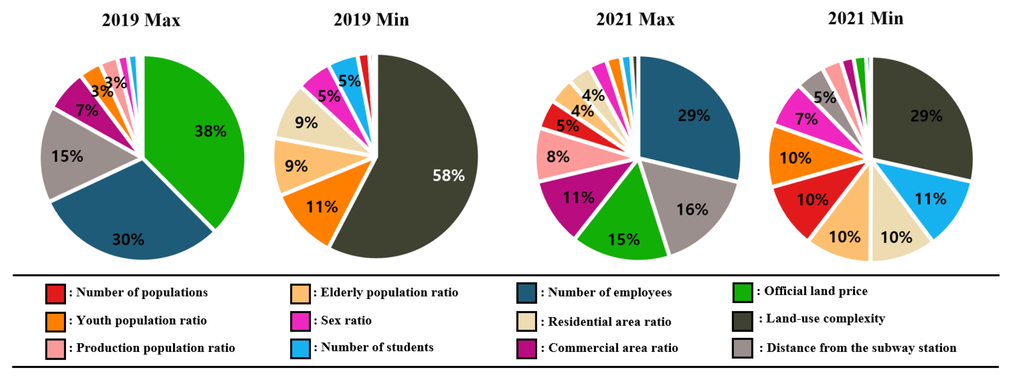
Figure 6 presents a variable importance map from the GRF model, highlighting the highest and lowest importance values across the grids. In addition,
Figure 7 depicts the area ratios of variables with the maximum and minimum importance values.
In the 2019 GRF model, the official land price emerged as the most significant variable influencing bus usage over the largest area. This variable was influential in the regions surrounding the Hangang River and Geumcheon-gu in eastern Seoul, encompassing approximately 38% of the city. Conversely, the number of employees was the dominant factor in northern and southern Seoul, covering about 30% of the area. The distance from the subway station was most significant in approximately 15% of Seoul, including Eunpyeong-gu, Guro-gu, and Yeongdeungpo-gu.
In the 2021 GRF model, the number of employees became the most influential variable, affecting northern Seoul in particular. This reflects the post-pandemic recovery of work-related trips, especially in areas with high employment density. Compared to the 2019 model, the area where the official land price was a crucial determinant experienced the most reduction. The proportion of Seoul where the official land price was a critical factor decreased from 38% in 2019 to 15% in 2021. This decline likely reflects a weakening correlation between property value and travel behavior during the pandemic, as commercial areas became less active under social distancing policies.
The significance of the commercial area ratio, productive population ratio, and total population number increased markedly in 2021, indicating a shift in the relative importance of factors influencing bus usage regionally. These variables gained prominence as public transport demand became more aligned with population-driven and locally essential activity patterns during the pandemic.
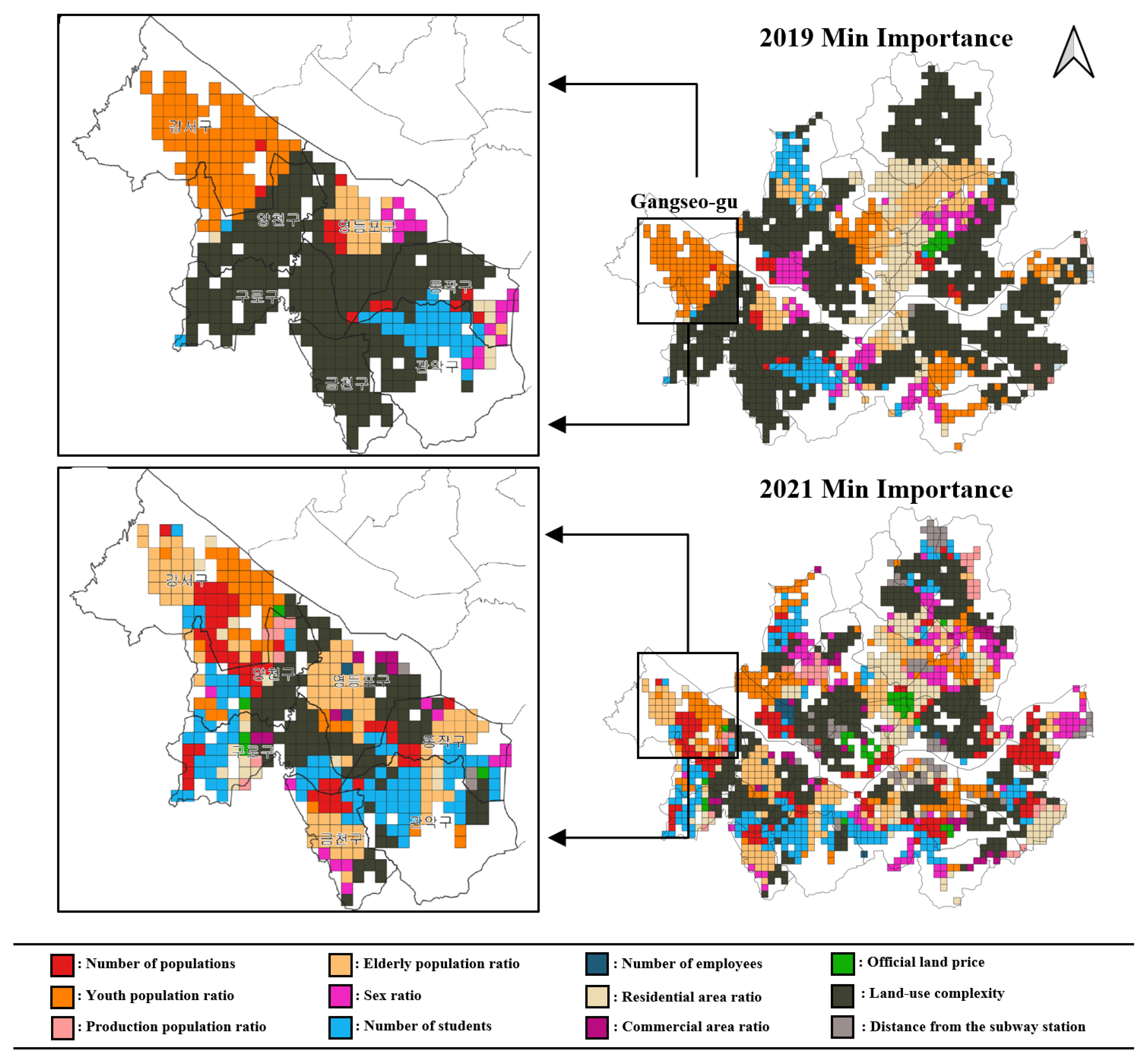
In contrast, land-use complexity was not a major determinant in the 2019 GRF model, with less significant influence than the youth and over-65 population ratios. Specifically, land-use complexity was the least critical variable, affecting 58% of Seoul. The youth population ratio was significant in only 11% of the area, predominantly around Gangseo-gu and Jongno-gu, whereas the over-65 population ratio was notable in just 9% of the area, primarily in central Seoul, from Gangbuk-gu to Seocho-gu.
For the 2021 GRF model, land-use complexity remained the least significant variable, followed by the number of students, residential area ratio, and over-65 population ratio. In 2021, the proportion of regions where land-use complexity was a minor factor decreased by half compared with 2019. Furthermore, a substantial increase occurred in areas where the number of students, total population, and distance from the subway station were insignificant. This trend reflects how the spatial determinants of bus ridership became more fragmented and context-dependent during the pandemic, underlining the differentiated impact of COVID-19 policies across neighborhoods. Overall, the changing influence of each variable between 2019 and 2021 demonstrates how the pandemic reshaped spatial travel demand patterns. Employment-related factors gained relevance, while traditional urban form indicators like land value and land-use complexity lost explanatory power, emphasizing the need for spatially adaptive transit planning.
This diversification in the importance of factors by region underscores the limitations of linear assumptions and the necessity of incorporating spatial considerations in public transportation demand studies.
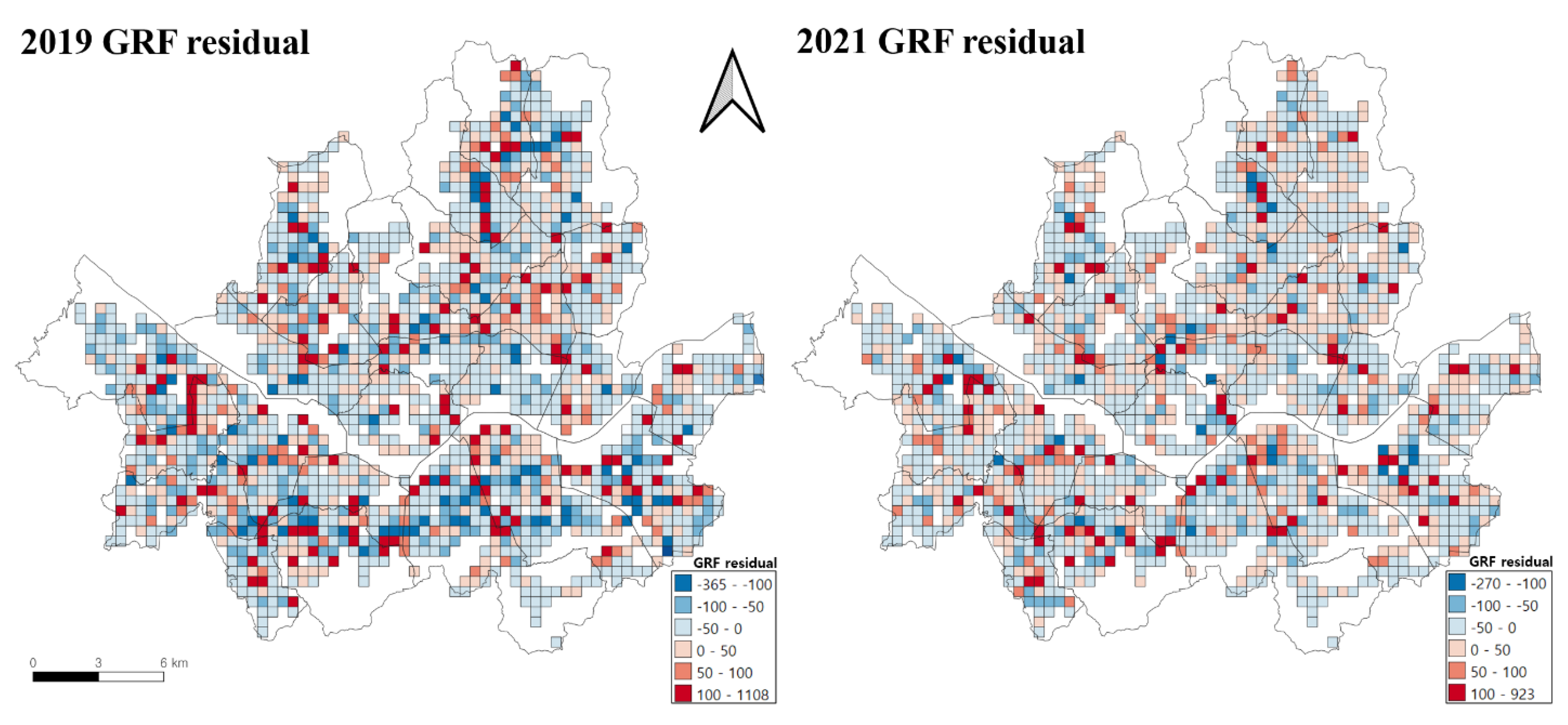
Figure 7 illustrates the proportion of each variable’s importance using pie charts. This figure presents the average significance of factors across the periods, providing insight into which factors were more influential during each one. Finally, an analysis of the residuals was conducted to evaluate the suitability of the GRF model. In addition,
Figure 8 depicts the spatial distribution of the GRF model residuals.
Figure 8 presents the residual map for both 2019 and 2021. The map indicates that the residuals are largely randomly distributed across the study area, with no clear spatial patterns emerging in either period. Moran’s I values for the GRF model residuals were 0.069 for 2019 and −0.005 for 2021. These values suggest a lack of significant spatial dependence, implying that the model adequately captured the major spatial patterns in bus ridership and that there were no residual spatial effects that could be explained by other factors.
5. Discussion
The COVID-19 pandemic presented new challenges for public transportation systems, particularly for vulnerable populations who depend heavily on public transit. In Seoul, bus networks serve as a crucial link for reaching destinations that are not directly accessible by subway, offering flexible mobility options for various demographic groups. This study provides spatial insights into how public bus usage changed during the pandemic and reveals the localized effects of key influencing factors.
Our findings are consistent with prior studies that observed pandemic-induced changes in transit demand patterns [
6,
9,
21], but they extend existing knowledge by incorporating spatial heterogeneity using multiscale geographically weighted regression (MGWR). Previous research has established that demographic and built-environment variables significantly impact public transportation use [
1,
15,
21,
22]. However, our results highlight that these impacts vary considerably across neighborhoods, especially in the context of post-COVID-19 recovery. Unlike conventional models that rely on spatially uniform assumptions, MGWR reveals the nuanced and region-specific nature of these relationships.
From a methodological standpoint, this study compares the performance of GWR and MGWR and demonstrates that MGWR more effectively captures spatial variation by applying variable-specific bandwidths. The analysis shows that, for instance, the influence of population size increased in certain northern districts of Seoul after the pandemic, while the influence of the over-65 population declined, likely due to behavioral and demographic shifts. Similarly, the reduced demand from students was reflected in areas where remote learning became widespread. These results suggest that pandemic-related behavioral changes have altered the spatial dynamics of transit use. Our findings indicate that COVID-19 policies, such as curfews and telecommuting recommendations, led to short-term changes in structural variables like land-use complexity and public transportation accessibility. These policies influenced behavioral patterns, such as reduced commuting and increased remote work, which in turn affected the demand for public transportation. The interplay between these behavioral changes and structural variables highlights the complex dynamics of urban mobility during the pandemic. Understanding these interactions is crucial for designing adaptive transportation strategies in future urban planning.
This
Figure 9 illustrates the spatial patterns observed in the study, highlighting the areas where the influence of demographic and land-use factors on public bus demand shifted over time.
Complementing the MGWR analysis, the machine learning-based geographical random forest (GRF) model provided additional depth by capturing both nonlinear relationships and spatial dependencies. In contrast to the standard random forest (RF) model, GRF incorporated spatial bandwidths, uncovering regionally distinct determinants of bus usage in both pre- and post-pandemic periods. For instance, while land price, employment density, and subway accessibility were highly influential in 2019, their importance declined in 2021, with other variables gaining prominence. This shift illustrates the evolving drivers of transit demand and underscores the value of combining statistical and machine learning approaches in spatial transport research.
From a policy and planning perspective, the findings offer several practical implications. First, the spatially disaggregated results support the design of locally adaptive transit strategies. Transit planners can tailor bus routes and service frequencies based on regional differences in demographic and land-use profiles. For example, areas where demand from older adults has increased could receive enhanced service coverage, while service in areas with declining student ridership might be reduced to optimize resource allocation. Such dynamic planning promotes both efficiency and equity—critical goals in resilient public transport systems.
Furthermore, integrating MGWR and GRF into transport analysis enables policymakers to move beyond one-size-fits-all approaches and implement context-sensitive interventions. These methods provide planners with tools to identify high-priority regions for intervention and tailor responses according to the spatial variability of influencing factors. In future pandemics or disruptions, such tools could be instrumental in designing scalable and responsive transit strategies that maintain service quality while minimizing public health risks.
While this study focuses on Seoul, its methodological framework is transferable to other metropolitan areas with similar transit infrastructures. The combined use of MGWR and GRF allows for localized insight into urban mobility systems and could be adopted in comparative studies across different cities. However, contextual differences in governance, urban form, and travel behavior must be considered when applying this approach elsewhere.
Regarding the methodological contributions, this study compared the performance of multiple models, including GWR, MGWR, RF, and GRF, to determine which model is most suitable under varying conditions. Each of these models offers distinct advantages depending on the context of the study. For example, GWR is effective when spatial variation is moderate and can capture local dynamics, but it may not handle complex spatial dependencies as well as MGWR. The MGWR approach, which applies variable-specific bandwidths, performs better when there are substantial regional differences in influencing factors, as observed in the post-pandemic period. Meanwhile, RF excels at uncovering nonlinear relationships between variables but does not explicitly account for spatial dependencies, which is a limitation for studies focused on densely populated urban areas. On the other hand, GRF, by incorporating both spatial and nonlinear dependencies, provides the most comprehensive insights for understanding urban transit patterns in complex metropolitan settings.
This comparative analysis of the models contributes to the broader field of transport research by illustrating the strengths and weaknesses of each approach in handling spatial-temporal data. By understanding which model is most appropriate for different circumstances, transit planners and researchers can make more informed decisions when selecting the methodology for future studies or planning efforts.
This study has several limitations. It primarily analyzes bus usage as a proxy for public transport demand and does not account for multimodal interactions or temporal fluctuations (e.g., hourly or daily patterns). Future research could incorporate subway data or real-time mobility datasets to enhance understanding of multimodal dynamics. Moreover, applying this methodology across multiple cities could validate its generalizability and inform broader urban transport policy. It is also unclear how COVID-19 policies impacted structural variables like land-use complexity and public transportation accessibility in the short term. While changes observed were assumed to be due to pandemic policies, it is uncertain whether these changes were directly linked to COVID-19 or other factors such as population shifts or trends in transportation modes. Moreover, the full recovery of COVID-19 impacts by 2021 remains uncertain, especially in regions affected by secondary waves. Data from 2022 could have provided more clarity, particularly regarding shifts in transportation modes, which might have been influenced by both pandemic policies and pre-existing trends. Finally, the limited data available for this study may have constrained the conclusions. Expanding data sources in future studies could lead to more robust and generalizable findings.
In summary, this study contributes to the literature by revealing localized shifts in transit demand patterns through advanced spatial modeling. By identifying the most influential factors and their regional variations, the findings support more targeted and equitable transportation planning in the post-pandemic era.
6. Conclusions
This study identifies spatial inconsistencies in public transportation usage and explores the factors with the most significant influence by region and the spatial changes before and after the pandemic. By systematically identifying the spatial heterogeneity of Seoul city bus demand before and after the pandemic through multiscale geographically weighted regression (MGWR) and geographic random forest (GRF), we have significantly contributed to the theoretical advancement of transportation demand theory, particularly in understanding spatial dynamics within urban transit systems. The combination of MGWR and GRF enables a more nuanced view of the complex, region-specific patterns of transit demand, revealing how the influence of key factors shifts over time and across locations.
From a methodological perspective, this study advances the use of spatial modeling by demonstrating the advantages of integrating both traditional regression-based approaches (GWR) and machine learning methods (GRF). The GRF model, by highlighting changes in the importance of specific variables, provides deeper insights into the evolving factors influencing bus capacity, while GWR clarifies the regional variations in these relationships. This hybrid approach enhances both theoretical and methodological frameworks for future spatial transport research, especially in the context of post-pandemic mobility analysis.
In practical terms, our findings provide actionable guidance for urban planners and policymakers. The identification of region-specific shifts in transit demand due to the pandemic can aid in tailoring public transport policies to accommodate evolving needs. For example, understanding the dynamics of bus usage in specific districts can lead to more responsive and adaptive public transport strategies, ensuring efficient resource allocation and service provision. Moreover, by focusing on the spatial variability of demand, this research offers a blueprint for designing future transport systems that can better withstand disruptions like pandemics.
For future research, several directions are suggested. First, as part of the metropolitan area, Seoul has extensive public transportation exchanges with surrounding regions (Gyeonggi and Incheon). Future studies should include these areas to provide a more comprehensive view of regional interactions and dynamics. The lack of bus data from Gyeonggi and Incheon limited the analysis. Expanding the study to include the entire metropolitan area could offer more robust insights for public transportation policies during pandemics. Additionally, analyzing bus usage by time of day is essential, as travel purposes vary significantly by time (e.g., morning/evening commutes vs. nighttime travel). Understanding temporal changes in bus usage patterns could further reveal the impact of COVID-19 on daily mobility behavior and help predict changes in transport demand under non-pandemic situations. This research approach could also be instrumental in facilitating more rapid and effective responses to future public transport challenges, both pandemic-related and otherwise.


