Article

Does a Time-Lagged Effect Exist Between Landscape Pattern Changes and Giant Panda Density?

Shaanxi Key Laboratory of Qinling Ecological Security, Shaanxi Institute of Zoology, Xi’an 710032, China
*
Authors to whom correspondence should be addressed.
Land 2025, 14(5), 1075; https://doi.org/10.3390/land14051075
Submission received: 20 March 2025 / Revised: 6 May 2025 / Accepted: 13 May 2025 / Published: 15 May 2025
(This article belongs to the Special Issue Landscape Fragmentation: Effects on Biodiversity and Wildlife)

Abstract

:
Land use and land cover change (LULCC) can influence giant panda distributions by altering landscape structure and configuration. However, the spatial impacts and potential time lag effects of landscape pattern changes on giant pandas remain underexplored. In this study, we applied a random forest classification method to analyze LULCC in 1990, 2000, and 2010, alongside calculating a set of landscape metrics to assess changes in landscape fragmentation, connectivity, and diversity. Random forest regression models were then used to evaluate the spatial relationships between landscape metrics and giant panda density, with the aim of identifying whether a time lag effect exists. The results revealed the following: (1) The random forest classification achieved high land use classification accuracy. Forests remained the dominant land cover, occupying approximately 97% of the study area throughout the period, with only minor fluctuations observed among other land use types. (2) Landscape metrics indicated increasing landscape fragmentation, connectivity, and diversity. While increased landscape fragmentation can negatively impact giant panda habitat, improvements in landscape connectivity and diversity could mitigate these effects by preserving movement corridors and enhancing habitat accessibility. (3) The strongest correlations between giant panda density and landscape metrics were observed when the time points aligned. Landscape metrics from 2010 showed the highest correlation with the 4th NGPS (around 2010), and landscape metrics from 2000 had the highest correlation with the 3rd NGPS (around 2000). The results revealed that giant panda density responded most strongly to contemporary landscape pattern changes, suggesting an immediate response. However, correlations with earlier landscape metrics also suggest that a relatively weak time lag effect may be present. All landscape metrics were derived from remote sensing data, enabling scalable and repeatable GIS-based analysis. These findings highlight the utility of spatial landscape indicators for monitoring species distribution patterns and underscore the importance of maintaining and enhancing habitat connectivity within giant panda conservation efforts.

1. Introduction

The giant panda (Ailuropoda melanoleuca) serves as a flagship species for biodiversity conservation efforts. While considerable progress has been made in giant panda protection in China, various challenges persist. Anthropogenic activities, climate change, environmental pollutants, and pathogen spread continue to threaten their populations and habitats [1].
Many factors affect giant panda distribution, including biotic and abiotic factors. These factors include the giant panda population baseline, age structure, sex ratio, birth-death rate, bamboo distribution and regeneration, forest ecosystem structure, human interference, and climate change. However, many of these factors are difficult to obtain consistently across large regions and long time spans. As remote sensing and spatial analysis technologies advance, spatial data (e.g., climate variables and land cover data) offer a scalable, repeatable, and increasingly accessible alternative for monitoring habitat changes and predicting species distributions. Climate change was previously considered a primary driver because it strongly affects the spatial and temporal distribution of bamboo—the staple food of giant pandas—as well as the structure and continuity of forest ecosystems. For example, changes in temperature and precipitation influence bamboo growth cycles, flowering, and regeneration patterns, which in turn shape giant panda movement and habitat selection across landscapes [2,3]. Moreover, climatic variability can alter habitat suitability at broad spatial scales, making it a key concern in earlier ecological assessments [4]. However, recent studies have noted that while climatic factors historically exert the most significant influence on the giant panda distribution, their relative importance is declining in the face of intensified land use changes and anthropogenic disturbances [5,6]. Wang et al. [7], for instance, emphasized that forest cover—closely tied to land use—now exerts a stronger influence on giant panda persistence than climate change. This transition underscores the growing significance of land use and land cover change (LULCC) and landscape pattern alterations, which can rapidly fragment habitats and reduce connectivity even without major climate shifts.
LULCC can profoundly alter the composition and configuration of the landscape, thereby influencing landscape fragmentation, connectivity, and diversity [8]. Research on LULCC and landscape pattern changes can help us understand the distribution of giant pandas and changes in their habitats. With the aid of the geographic information system (GIS) and remote sensing, changes in landscape structure can be quantitatively described through landscape metrics, which have been widely used to study population declines or extinction [9], species population distributions [10,11], species richness [12,13], biodiversity, ecosystem services, and wildlife habitat suitability [13,14,15,16,17,18]. In giant panda studies, Wang et al. [19] examined the relationships between landscape metrics and the pseudo-absence of the giant panda. Liu et al. [20] qualitatively analyzed the relationships between landscape metrics and giant panda distributions. Qin et al. [21] evaluated the relationships between landscape metrics and the number of giant pandas in Sichuan Province. However, a quantitative evaluation of the relationships between landscape metrics and giant panda density in the Qinling Mountains is lacking. Moreover, most previous studies have assumed that species distributions respond immediately to changes in landscape patterns, without considering possible time lag effects. However, ecological responses to environmental changes often exhibit temporal delays—a phenomenon referred to as the time lag effect. This concept has been widely discussed in the ecological literature, including studies on the dynamic changes in predators and prey [22], the response of vegetation to climate change [23,24], and disease transmission [25]. In the context of landscape ecology, time lags may arise because biological processes such as dispersal, reproduction, and habitat colonization occur gradually over time [26,27,28,29]. For giant pandas, time lag effects may be especially relevant given their low reproductive rates, strong habitat specificity, and limited mobility [30,31]. These traits can lead to demographic inertia, where population adjustments to environmental changes take years to manifest [32]. In addition, giant pandas may exhibit short-term behavioral buffering (e.g., range shifts or altered movement patterns) or may persist temporarily in degraded habitats, masking early impacts of habitat loss. Therefore, even when habitat conditions improve or deteriorate, the full ecological impact on giant panda density may not be immediately observable. If these lagged responses are overlooked, the role of landscape pattern changes may be underestimated or misinterpreted, potentially leading to ineffective or mistimed conservation interventions.
In this context, the present study does not aim to build a comprehensive ecological model incorporating all known drivers of giant panda distribution. Instead, it seeks to evaluate the potential of landscape metrics derived from remote sensing as spatial proxies for assessing changes in giant panda distribution over time. These metrics, derived from remotely sensed LULCC data, are increasingly available, reproducible, and scalable across regions and time periods—offering a practical and technology-driven approach for habitat evaluation, especially in remote or data-limited areas. Building on this spatial perspective, we aimed not only to examine the spatial relationships between landscape metrics and giant panda density but also to explore whether time lag effects exist in how giant pandas respond to landscape pattern changes. Incorporating time lag analysis into landscape studies allows us to distinguish between immediate and delayed responses, thereby improving the accuracy of ecological inference. This distinction is essential to avoid overestimating short-term stability or underestimating long-term landscape impacts. Understanding whether and how delayed responses occur is crucial for designing scientifically informed and temporally appropriate conservation measures to support the stability and long-term viability of giant panda populations.
The specific objectives of this study included (1) analyzing LULCC in 1990, 2000 and 2010; (2) analyzing landscape pattern changes on the basis of landscape metrics in 1990, 2000 and 2010; and (3) exploring the relationship between landscape pattern changes and giant panda density, and determining whether a time lag effect existed. A GIS-based approaches to quantify and model landscape pattern changes provide valuable insights into how spatial fragmentation, patch configuration, and habitat connectivity affect giant panda distribution. Our study adopts this landscape perspective to better understand the role of spatial structure and its changes in shaping giant panda density patterns.

2. Materials and Methods
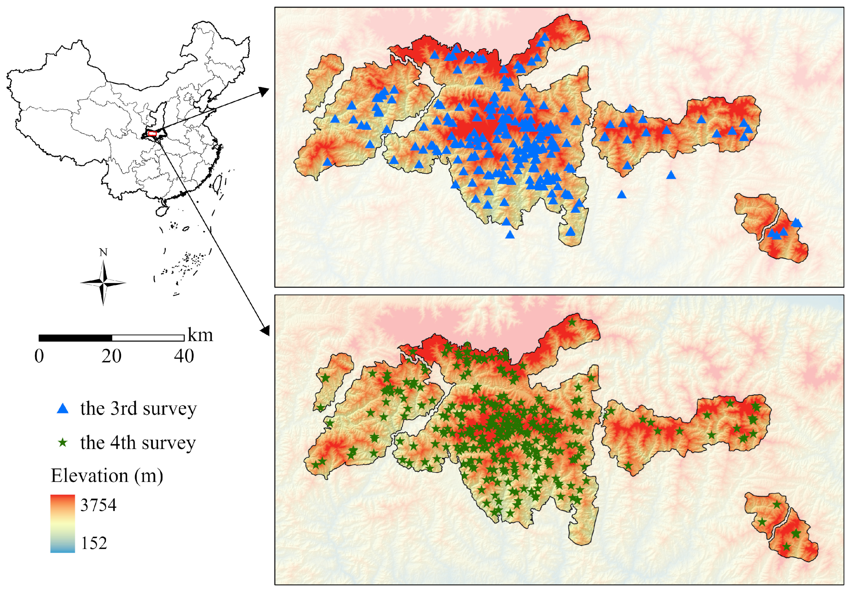
2.1. Study Area

This study focuses on the Qinling Mountains in Shaanxi Province, China (105°29′18″–111°01′54″ E, 32°28′53″–34°32′23″ N) (Figure 1). The Qinling Mountains are the dividing line between the northern and southern climates in China. The mountain range has the highest latitudinal distribution of giant pandas in China, with the population density ranking first in the country. The southern slope is relatively gentle, with a total length of 100–130 km. The northern slope is steep, and the total length is less than 40 km. The elevation ranges from 185 to 3771.2 m above sea level. Characterized by a continental monsoon climate, the Qinling Mountains have an average annual temperature of 12–17 °C. The average annual rainfall is approximately 820 mm, of which more than 60% falls between June and September. Deciduous broadleaf and subtropical evergreen forests are mainly found at low elevations, while temperate broadleaf and subalpine coniferous forests are found at mid-elevation, and subalpine scrub meadows are found at high elevations [33].

2.2. Random Forest Classification and Regression Models

Random forest (RF) is an ensemble machine learning algorithm comprised of many classification or regression trees, making it robust to random and systematic label noise and reducing the chance of model overfitting. Remote sensing and earth observation-based approaches, coupled with machine learning models, are recognized as the most efficient, practical, real-time, and accurate solutions for developing spatially explicit models of wildlife habitats [34]. Ma et al. [35] reported that RF models are generally characterized by having the highest mean classification accuracy. Moreover, RF also has strong predictive capabilities in regression models [36]. In this study, an RF classification model was employed to analyze the dynamic changes in landscapes in the Qinling Mountains using satellite images from 1990 to 2010. Additionally, an RF regression model was applied to evaluate the relationship between giant panda density and landscape metrics.
RF models build numerous trees in an iterative way from random samples of the training data. The ensemble of the predictions of all trees constitutes the final model. RF classification trees are applied to discrete variables, and RF regression trees are applied to continuous variables. RF requires users to make decisions about two tuning parameters: the number of trees to grow (ntree) and the number of variables to randomly sample as candidates at each split (mtry). Through parameter tuning, RF aims to maintain the prediction strength while inducing diversity among the trees [37]. In this study, the default values were used in RF modeling because previous researchers have shown that the sensitivity of the user-defined parameters is minimal and that the default values are often a good choice [36]. Thus, mtry was set to one-third of the predictive variables, and ntree was set to 500. The RF model was implemented on the Google Earth Engine platform and “randomForest” package in R software (version 4.2.0).

2.3. Giant Panda Density Data

This study used individual-based giant panda distribution data from the 3rd and 4th National Giant Panda Surveys (NGPSs) in the Qinling Mountains. The field surveys were conducted from November 2000 to June 2001 (3rd NGPS) and from March 2012 to July 2013 (4th NGPS). Field data were collected along pre-set transects, each with a length of no less than 2 km. Survey teams recorded direct sightings and indirect evidence of giant pandas, including feces, dens, sleeping sites, and footprints. In the Qinling Mountains, 1749 occurrence points were obtained from the 3rd NGPS [38], and 2004 occurrence points were obtained from the 4th NGPS [39].
Individual giant panda numbers were estimated using the “combined distance and bamboo-bite length method”. This approach distinguishes individuals based on (1) the spatial distance between fecal samples, under the assumption that giant pandas have limited daily movement, and (2) differences in the average length of bamboo fragments remaining in feces, which reflect individual feeding patterns. For cubs, population estimates were inferred from observed birth rates. In the 4th NGPS, non-invasive genetic methods (DNA analysis) were also used as a supplementary means of individual identification.
A total of 273 individuals were identified in the 3rd NGPS and 345 in the 4th NGPS. These individual locations were used to calculate spatial density using kernel density analysis in ArcGIS 10.8 (Esri Inc., Redlands, CA, USA), resulting in continuous raster layers representing giant panda density in 2000 and 2010 (Figure 2).

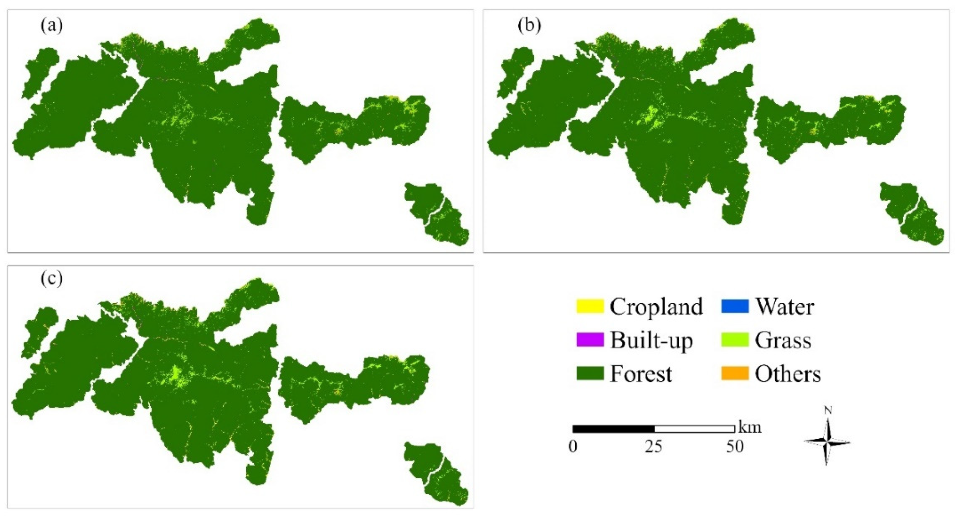
2.4. Land Cover Classification

We used the Landsat 5 Thematic Mapper (TM) to map land cover in 1990, 2000, and 2010. The Landsat Level 2, Collection 2, Tier 1 data were obtained and processed on the Google Earth Engine platform. For each target year, we created an image stack for the target year ± two years (e.g., images from 2008 to 2012 for the year 2010) to minimize missing data and cloud interference. Images were selected from June to September during the vegetation growth period. Various spectral indices were calculated and appended to the cloud-free stacks along with topographic information (aspect, slope, and elevation) for land cover classification. This topographic information was obtained from a digital elevation model with a spatial resolution of 30 m on the Google Earth Engine platform.
Our classification system included six land cover classes: forest, cropland, grass, built-up, water, and “others” (Table 1). We selected sample data by visual interpretation and field investigation. RF classification models (see Section 2.2) were used to classify the Landsat images. We randomly selected 70% of the sample data for classification using the RF algorithm and selected the remaining 30% for validation. Using the validation dataset, we calculated four confusion matrices (one per epoch) to determine the overall accuracy (OA), producer accuracy (PA), and user accuracy (UA) of land cover classification. Additionally, a nonparametric kappa coefficient test was used to measure the degree of classification accuracy.

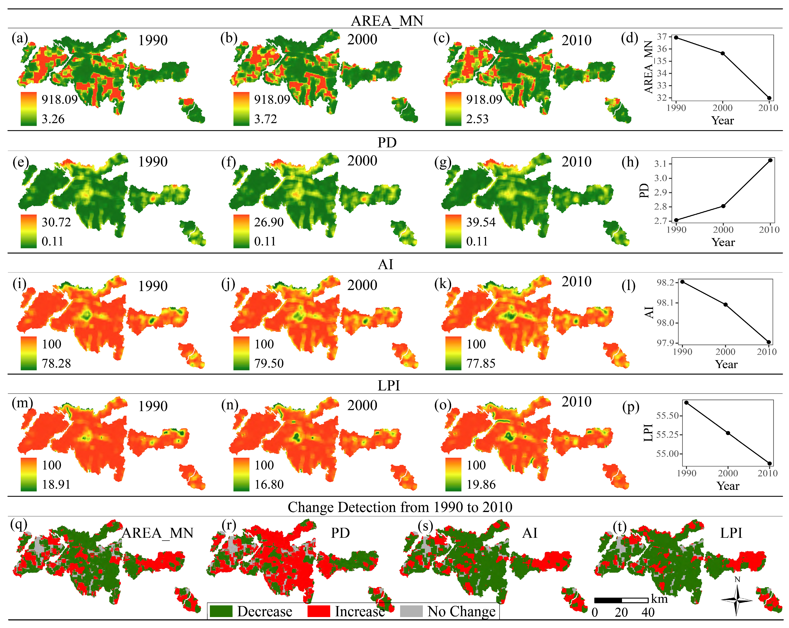
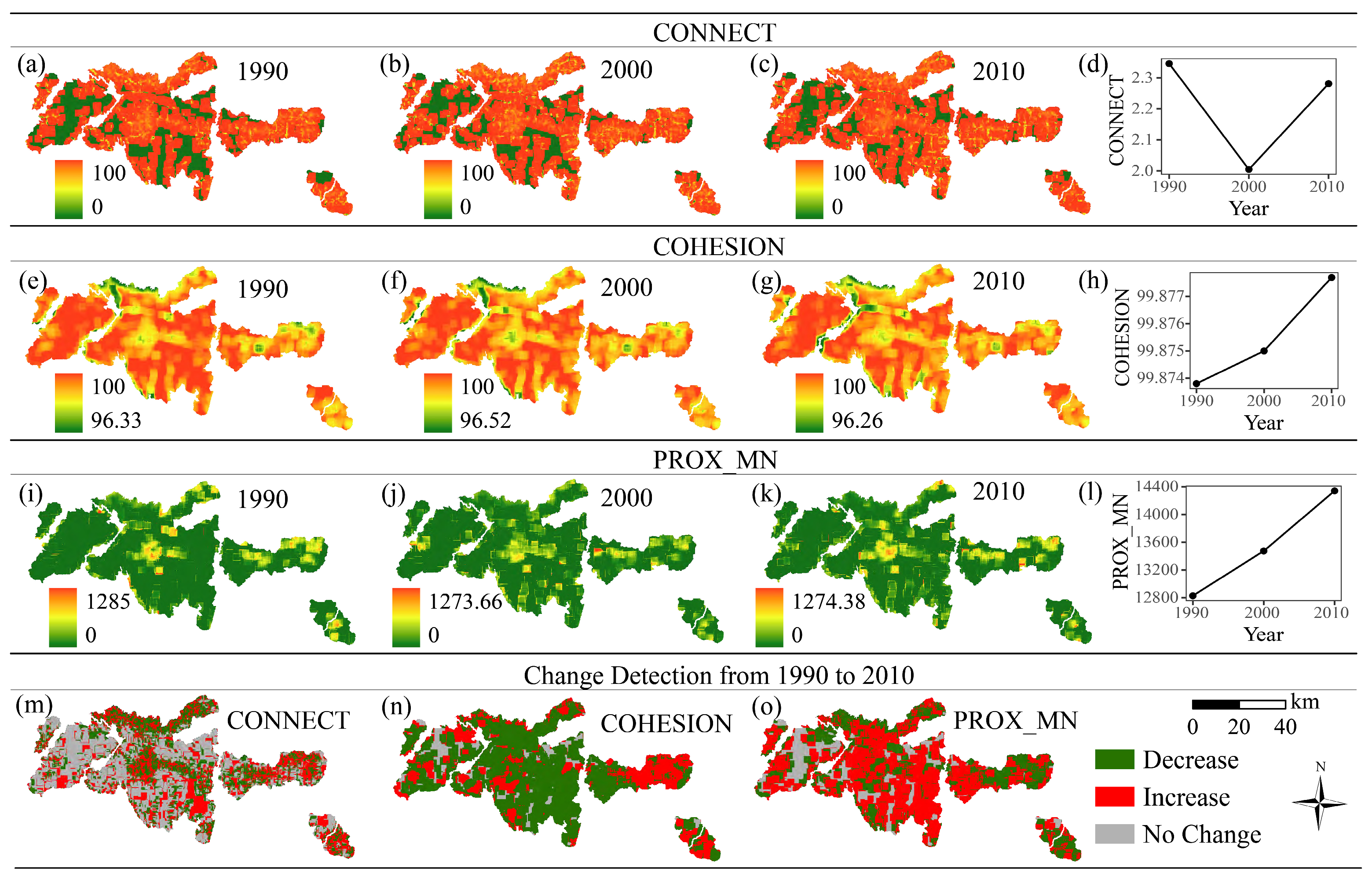
2.5. Landscape Metric Determination

An open-source software program, FRAGSTATS (version 4.3), was used to calculate landscape metrics in this study, and an 8-cell neighborhood rule was followed to define patches [40]. The software computes landscape metrics using a moving square window with a radius of 3 km as the appropriate scale and creates a continuous landscape metric surface for statistical analysis [19]. This moving window was supported by both previous empirical studies and the ecological behavior of the target species. Wang et al. [19] tested various window sizes and found that most landscape metrics stabilized at a radius of 3–3.5 km in giant panda habitats. This result indicates that a 3 km window is an appropriate scale for landscape analysis in such environments. Additionally, this scale aligns well with the maximum daily movement distance of the giant panda, which is approximately 3 km [6]. Together, these factors provide strong empirical and ecological support for our chosen analytical scale. The metrics measured were the mean area (AREA_MN), patch density (PD), largest patch index (LPI), aggregation index (AI), mean proximity index (PROX_MN), patch cohesion index (COHESION), connectance index (CONNECT), Shannon’s diversity index (SHDI), and Shannon’s evenness index (SHEI). A description of the landscape metrics can be found in Table S1. We chose these metrics because they are commonly used in literature and represent landscape fragmentation, connectivity, and diversity [16,19,41,42,43]. All landscape metrics used in this study were derived from land use and land cover datasets, enabling scalable and repeatable remote sensing-based analysis.

2.6. Time Lag Effects of Landscape Metrics on Giant Panda Density

To explore whether there was a time lag effect of landscape pattern changes on the giant panda distribution, we constructed a series of random forest regression models to analyze the relationship between landscape metrics and giant panda density in different time series. Specifically, we modeled (1) giant panda density from the 4th NGPS (around 2010) against landscape metrics from 2010 (no lag), 2000 (~10 years lag), and 1990 (~20 years lag); and (2) giant panda density from the 3rd NGPS (around 2000) against landscape metrics from 2000 (no lag) and 1990 (~10 years lag). Our choice of a 10-year lag interval was guided by two main considerations. First, while we recognize that ecological lag periods can vary depending on species traits and environmental conditions, previous studies have shown that demographic and ecological responses to habitat change often emerge over multi-year or even decadal time frames [28]. A 10-year window thus represents an ecologically meaningful time scale for detecting potential delayed effects of landscape change. Second, this time interval aligns with the timing of the giant panda surveys, which are the most comprehensive and consistent data sources available on giant panda distribution and density at a large scale. The 3rd and 4th NGPSs were conducted approximately 10 years apart, providing fixed and comparable reference points for assessing both immediate and delayed responses to landscape changes. By comparing model performance, we assessed whether contemporary or historical landscape configurations better explained giant panda density patterns, thereby evaluating the potential presence of time lag effects. This approach follows the best practices in lag effect research, which uses time-staggered environmental predictors to detect delayed species or population responses [44,45]. Random forest models are particularly well-suited for this analysis, as they can effectively capture complex nonlinear relationships between variables and provide estimates of the relative importance of each predictor. This approach allowed us to assess whether giant panda density was better predicted by current or past landscape configurations, thereby providing insights into the existence and strength of ecological time lag effects. Moreover, this spatially detailed modeling framework allows for fine-scale analysis of habitat patterns and their changes over time, supporting the identification of landscape features that may influence species distribution and enabling a more efficient, data-driven approach to habitat monitoring and assessment.
All statistical analyses were completed using R software (version 4.2.0).

3. Results

3.1. Land Use and Land Cover Change

The overall accuracies of the 1990, 2000, and 2010 images were 97.38%, 97.55%, and 97.44%, respectively, with kappa coefficients of 0.9544, 0.9578, and 0.9558, respectively (Table 2). This indicates the reliability and stability of the LULCC change analysis and the maps produced.
The results of the land cover analysis from 1990 to 2010 revealed that the landscape composition in the study area remained largely stable, with forests consistently dominating the region, covering approximately 97% of the total area (Table 3, Figure 3). However, slight changes were observed across other land cover types.
Forest area decreased from 3500.90 km2 in 1990 to 3478.53 km2 in 2010, indicating an absolute loss of 22.37 km2 and a percentage decrease of 0.64% over the 20-year period. Despite this reduction, forests remained the predominant land cover. Grassland expanded from 76.89 km2 to 83.39 km2, representing an increase of 8.45%. Cropland increased from 8.87 km2 to 22.62 km2, marking a substantial absolute gain of 13.75 km2 and a relative increase of 155.01%. The “Others” land use type grew from 6.55 km2 to 8.10 km2, a rise of 23.66%. Built-up land exhibited an increase of 0.09 km2 (from 2.31 km2 to 2.40 km2), equivalent to a 3.90% growth. Water bodies, though small in extent, more than doubled in area from 0.34 km2 to 0.83 km2, with an increase of 0.49 km2 and a percentage rise of 144.12%. Despite the high percentage increases observed in cropland and water, their absolute areas remained relatively small compared to forest. Consequently, these changes had limited influence on the overall landscape structure.

3.2. Changes in Landscape Metrics

The landscape metrics AREA_MN, PD, AI, and LPI were selected to represent landscape fragmentation. AREA_MN, AI, and LPI decreased, whereas PD tended to increase from 1990 to 2010 (Figure 4). These findings indicate that both the mean areas and largest patches are decreasing, and that landscape fragmentation is intensifying.
Change detection maps reveal the extent of these shifts more precisely. For AREA_MN, 57.09% of the study area experienced a decrease, while only 32.60% showed an increase. Similarly, AI and LPI decreased in 65.39% and 69.17% of the area, respectively. For PD, 57.09% of the area increased, further supporting the conclusion of reduced dominance of large patches.
The spatiotemporal changes in CONNECT, COHESION, and PROX_MN, which are related to landscape connectivity, are shown in Figure 5. From 1990 to 2010, CONNECT first decreased but then increased. The area with low CONNECT values decreased in the western and southern parts of the study area. Ultimately, CONNECT exhibited a relatively more stable pattern, with 42.95% of the area showing no change, while 27.26% decreased and 29.79% increased. COHESION and PROX_MN increased from 1990 to 2010. Although the change detection map of COHESION shows a 67.18% decrease (Figure 5n), the average value of its spatial distribution in each stage shows an upward trend from 1990 to 2010 (Figure 5h). PROX_MN increased in 57.27% of the area, implying that the spatial proximity between patches improved in some regions, potentially due to the emergence of new small patches or changes in patch distribution patterns. These changes in landscape metrics indicate increases in the connectivity and continuity of the landscape.
The landscape metrics SHDI and SHEI are related to landscape diversity. SHDI and SHEI tended to increase from 1990 to 2010 (Figure 6). SHDI increased in 70.04% of the region, and SHEI increased in 65.88%, indicating a rise in land cover variety and more balanced distribution of patch types across the study area. These findings suggest that landscape diversity improved over the study period.

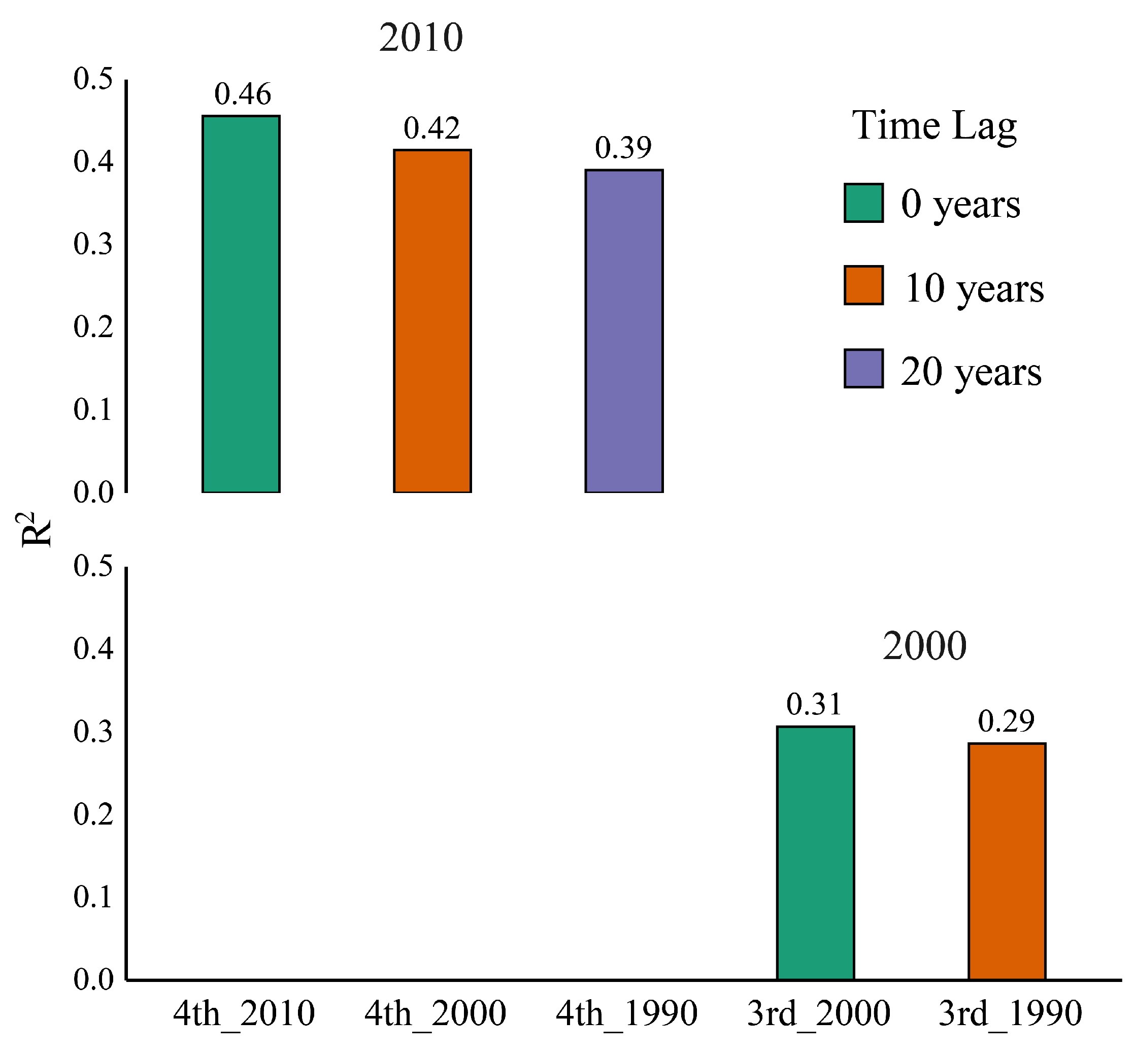
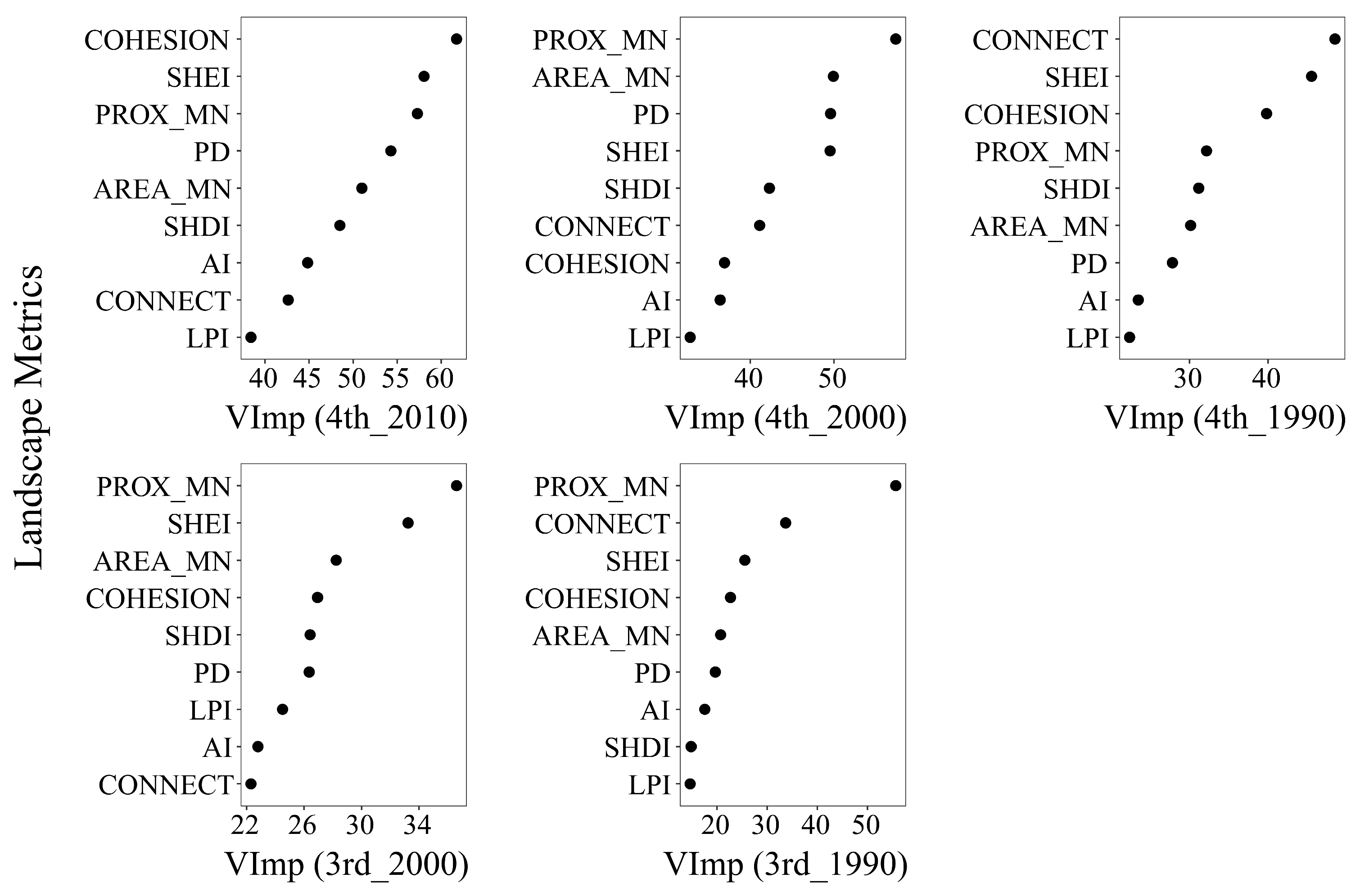
3.3. Does a Time Lag Effect Exist?

The random forest models were used to calculate the relationship between giant panda density and landscape metrics during different periods. The results indicated that the relationship between the giant panda density in the 4th survey (conducted around 2010) and landscape metrics in 2010 (R2 = 0.46) was greater than that between the giant panda density in the 4th survey and landscape metrics in both 2000 (R2 = 0.42) and 1990 (R2 = 0.39) (Figure 7). Similarly, the relationship between the giant panda density in the 3rd survey (conducted around 2000) and landscape metrics in 2000 (R2 = 0.31) was greater than that between the giant panda density in the 3rd survey and landscape metrics in 1990 (R2 = 0.29) (Figure 7). The results showed that giant panda density was most strongly correlated with landscape metrics from the same period, indicating an immediate response to landscape pattern changes. However, moderate correlations with earlier landscape metrics suggest that a relatively weak time lag effect may also exist, potentially reflecting delayed population responses. Under the 10-year interval framework used in this study, changes in landscape patterns and species density appeared to be closely aligned overall.
To further examine the relative influence of landscape metrics on giant panda density, we assessed variable importance using random forest models, which highlight the potential of spatial pattern indicators in explaining species distribution. As shown in Figure 8, landscape connectivity and diversity metrics generally exhibited higher importance across all time points. Specifically, PROX_MN and SHEI were consistently ranked among the top contributors in explaining giant panda density, followed by COHESION, CONNECT, and SHDI. In contrast, fragmentation-related metrics such as PD, LPI, and AI demonstrated relatively lower importance. These results indicate that giant panda density is more strongly associated with metrics reflecting landscape connectivity and heterogeneity than with those capturing simple fragmentation.

4. Discussion

In this study, we analyzed LULCC and landscape pattern change trends and evaluated whether there was a time lag effect on giant panda density in the Qinling Mountains.
The LULCC results indicated that the forest area decreased while other land types increased from 1990 to 2010. Rapid socioeconomic development with intensive industrialization and urbanization and an increasing human population could cause fluctuations in LULCC [46,47]. Fortunately, in the late 1990s, the Chinese government promoted many conservation efforts to protect forest ecosystems, such as the implementation of the Natural Forest Conservation Program and the Grain for Green Program [7,20]. These protection policies are the primary factors that caused LULCC to fluctuate within a small range. The forest coverage remains high at approximately 97% in the study area. However, Li et al. [48] reported that high forest coverage alone does not equal high giant panda density. Giant pandas prefer moderate forest coverage with high bamboo density. Bai et al. [49] noted that forest structure and successional stage are crucial in the habitat selection of giant pandas. Some forests in the Qinling Mountains need to be tended and managed to accelerate the habitat restoration process and improve habitat quality [47].
LULCC directly reshapes landscape composition and configuration, thereby influencing habitat spatial structure and wildlife expansion or contraction. Lindborg and Eriksson [50] indicated that landscape change is considered an important driver of species extinction. In this study, landscape fragmentation reduced the availability and spatial continuity of suitable patches, which could affect the spatial patterns of giant panda occurrence. The home range of a giant panda is approximately 5.4 km2 for females and 8.5 km2 for males [51]. This range can meet the foraging and courtship needs of giant pandas. However, with increasing landscape fragmentation, the largest landscape area decreases (Figure 4), which may limit the ability of giant pandas to meet their spatial needs for foraging and mating [52]. These disruptions to spatial structure may result in isolation or even extinction of giant panda populations. When the wildlife habitat structure is disturbed, improving landscape connectivity is critical and effective for the communication and reconstruction of giant panda populations [49]. Gao et al. [16] also demonstrated that landscape connectivity and shape complexity are important for wildlife conservation. Our variable importance analysis indicates that landscape connectivity and diversity are consistently the most influential predictors of giant panda density (Figure 8), highlighting the value of these metrics as spatial indicators for habitat suitability. In contrast, landscape fragmentation metrics alone showed relatively limited explanatory power, possibly because moderate fragmentation does not necessarily hinder movement if connectivity remains high. Encouragingly, our study area exhibited improved landscape connectivity and diversity (Figure 5 and Figure 6), which may help buffer the negative effects of landscape fragmentation and facilitate movement, gene flow, and population stability [53]. These findings reinforce growing conservation strategies that prioritize landscape connectivity over merely establishing new reserves [51]. Effective and functional ecological corridors are critical measures for improving functional connectivity and supporting long-term species persistence [51,54,55]. Conservation measures, including the restoration of vegetation and bamboo, the reconstruction of road culverts and guardrails, the construction of road tunnels, and the closure of tourist attractions, have been proposed and recommended accordingly [54,56]. Importantly, our study contributes a spatially explicit, GIS-based perspective on how landscape structure—quantified through metrics derived from remotely sensed data—can serve as a practical proxy for evaluating species distribution dynamics. This approach is particularly valuable in remote or data-limited regions, where detailed ecological data (e.g., on bamboo or population demography) are often unavailable or costly to collect.
To evaluate the temporal dynamics of landscape effects, we further assessed the potential time lag effect on giant panda density. Results indicate that the giant panda density from the 4th NGPS (conducted around 2010) was most strongly associated with the landscape metrics in 2010. Similarly, the giant panda density from the 3rd NGPS (conducted around 2000) aligned most closely with the landscape metrics in 2000. The immediate effects of landscape pattern changes on giant pandas were most pronounced in these surveys. This finding is similar to that of Hämäläinen and Fahrig [57], who reported that landscape fragmentation had no time lag effect on lichen species density. When human or natural disturbances cause landscape changes, giant pandas migrate from disturbed habitats to undisturbed habitats in the short term. In addition, the sensitivity of giant pandas to the distribution of bamboo forests may lead to their immediate response to landscape changes. Conversely, the early stages of landscape pattern changes also affect the density of giant pandas. The correlations between landscape metrics in 1990 and 2000 and the giant panda density in the 4th survey reached 0.42. The correlation between landscape metrics in 1990 and the giant panda density in the 3rd survey reached 0.29. This result may be due to a time lag effect of landscape pattern changes on giant panda population sizes [58]. The density of giant pandas is influenced not only by their distribution but also by their number. Although landscape pattern changes can affect giant panda distributions immediately, their impact on population size is slow. Therefore, there is a correlation between the giant panda density and early landscape changes. The changes in giant panda density are affected not only by the current landscape pattern but also by the past landscape pattern, but the current landscape pattern changes have the greatest impact.
These results provide guidance for giant panda conservation. First, the importance of landscape changes for giant pandas should be recognized. In addition, landscape pattern changes in giant panda distribution areas should be reduced to avoid the destruction of their habitats. Second, once the habitat of giant pandas is inevitably damaged, corresponding protective measures should be taken as soon as possible to prevent a decrease in the giant panda population size [58]. These measures should include habitat restoration, the construction of ecological corridors to increase connectivity, and the expansion of habitat areas. The adverse effects of landscape pattern changes on giant pandas should be minimized to the greatest extent possible.
While our study provides new insights into how landscape patterns influence giant panda density, several uncertainties should be acknowledged. First, there is a temporal mismatch between the timing of field surveys (NGPSs in 2000–2001 and 2012–2013) and the land use data (2000 and 2010), which may introduce minor discrepancies in the alignment between species response and habitat condition. Although such mismatches are common in long-term ecological studies using remote sensing data, and we have attempted to mitigate this by incorporating lagged landscape metrics, some uncertainty remains. Second, the 10- and 20-year lag intervals used in this study may have been too coarse to detect more immediate or short-term responses, particularly for ecological processes that unfold over shorter time scales. While our results showed only a relatively weak time lag effect, this does not necessarily preclude the existence of such effects. Previous studies have shown that ecological lag periods can vary considerably depending on species traits, habitat dynamics, and the nature of disturbances [28,45,59]. Therefore, further research incorporating finer temporal resolution may help to better capture the potential time lag effects in giant panda responses to landscape change. Third, our analysis focused primarily on the explanatory power of spatial structure and did not incorporate other key ecological drivers such as bamboo availability, climate variability, or human disturbance. Although some of these effects may be indirectly captured by landscape structure, future research integrating additional variables will help refine predictive models. Despite these limitations, the present study demonstrates that spatial characteristics of the landscape—quantified through accessible and standardized metrics—provide valuable insights into species distribution patterns. For conservation practice, this approach offers a cost-effective, GIS-based framework for identifying spatial priorities, monitoring habitat dynamics, and supporting data-driven decision-making in landscape planning for species conservation.
In future studies, we will incorporate additional influencing factors (bamboo distribution, climate, and human interference) to better analyze the synergistic effects of landscape patterns and other environmental pressures (such as the cumulative impact of drought exacerbating habitat fragmentation). Furthermore, we propose to use high-resolution remote sensing data with shorter time intervals, combined with more frequent or real-time population surveys, to better capture the dynamic relationships between landscape changes and giant panda distributions and reduce the uncertainty of model inferences. This approach may also improve the detection of subtle or delayed ecological responses, including potential time lag effects that could not be captured under the current temporal framework.

5. Conclusions

In this study, we assessed LULCC and landscape pattern changes in the Qinling Mountains from 1990 to 2010, with a focus on their spatial relationship with giant panda density. The classification results indicated that the forest area decreased while the areas of other land types increased within a limited range. These changes altered landscape configuration, leading to increased landscape fragmentation, connectivity, and diversity. Although increased landscape fragmentation can degrade giant panda habitat quality, the concurrent rise in landscape connectivity and diversity can help buffer some of these negative effects by maintaining habitat accessibility and promoting movement between patches. Importantly, our analysis demonstrated that landscape metrics derived from remote sensing data can serve as effective spatial proxies for evaluating changes in giant panda density over time. The strongest correlations between landscape metrics and giant panda density occurred when the time points of both datasets aligned. Specifically, the giant panda density from the 4th NGPS had the highest correlation with landscape metrics in 2010, and the giant panda density from the 3rd NGPS had the highest correlation with landscape metrics in 2000. The results revealed that giant panda density is most strongly influenced by current landscape pattern changes, with limited evidence of a potential weak time lag effect.
Overall, our findings highlight the value of using scalable, GIS-based landscape metrics to monitor and evaluate habitat conditions for species like the giant panda, particularly in remote or data-limited regions. Rather than constructing a comprehensive ecological model, this study underscores the potential of accessible spatial indicators to inform species distribution assessments across time, supporting spatially informed conservation planning.

Supplementary Materials

The following supporting information can be downloaded at: https://www.mdpi.com/article/10.3390/land14051075/s1, Table S1: Landscape metrics selected in this study.

Author Contributions

Conceptualization, Q.Z. (Qingxia Zhao) and X.J.; methodology, Q.Z. (Qingxia Zhao); software, Q.Z. (Qifeng Zhu); investigation, Q.Z. (Qifeng Zhu), Y.C., and Y.L.; data curation, Q.Z. (Qingxia Zhao) and J.H.; writing—original draft preparation, Q.Z. (Qingxia Zhao); writing—review and editing, D.C.; supervision, X.J. All authors have read and agreed to the published version of the manuscript.

Funding

This research was jointly supported by the Science and Technology Program of Shaanxi Academy of Sciences (Program No. 2020k-24, 2021k-3, 2023k-19, 2023k-50) and Shaanxi Science and Technology Department (2024ZC-KJXX-042).

Data Availability Statement

The data presented in this study are available on request from the corresponding author. The data are not publicly available due to privacy restrictions.

Conflicts of Interest

The authors declare no conflicts of interest. The funders had no role in the design of the study; in the collection, analyses, or interpretation of data; in the writing of the manuscript; or in the decision to publish the results.

References

  1. Huang, Q.; Fei, Y.; Yang, H.; Gu, X.; Songer, M. Giant Panda National Park, a step towards streamlining protected areas and cohesive conservation management in China. Global Ecol. Conserv. 2020, 22, e00947. [Google Scholar] [CrossRef]
  2. Tuanmu, M.N.; Vina, A.; Winkler, J.A.; Li, Y.; Xu, W.; Ouyang, Z.; Liu, J. Climate-change impacts on understorey bamboo species and giant pandas in China’s Qinling Mountains. Nat. Clim. Chang. 2013, 3, 249–253. [Google Scholar] [CrossRef]
  3. Li, X.; Mao, F.; Du, H.; Zhou, G.; Xing, L.; Liu, T.; Han, N.; Liu, Y.; Zhu, D.E.; Zheng, J.; et al. Spatiotemporal evolution and impacts of climate change on bamboo distribution in China. J. Environ. Manag. 2019, 248, 109265. [Google Scholar] [CrossRef]
  4. Li, R.Q.; Xu, M.; Wong, M.H.G.; Qiu, S.; Sheng, Q.K.; Li, X.H.; Song, Z.M. Climate change-induced decline in bamboo habitats and species diversity: Implications for giant panda conservation. Divers. Distrib. 2015, 21, 379–391. [Google Scholar] [CrossRef]
  5. Tang, J.; Swaisgood, R.R.; Owen, M.A.; Zhao, X.; Wei, W.; Pilfold, N.W.; Wei, F.; Yang, X.; Gu, X.; Yang, Z.; et al. Climate change and landscape-use patterns influence recent past distribution of giant pandas. Proc. R. Soc. B Biol. Sci. 2020, 287, 20200358. [Google Scholar] [CrossRef]
  6. Li, Y.; Rao, T.; Luo, G.; Price, M.L.; Liu, Y.; Ran, J. Giant pandas are losing their edge: Population trend and distribution dynamic drivers of the giant panda. Glob. Chang. Biol. 2023, 29, 4480–4495. [Google Scholar] [CrossRef]
  7. Wang, Y.; Lan, T.; Deng, S.; Zang, Z.; Zhao, Z.; Xie, Z.; Xu, W.; Shen, G. Forest-cover change rather than climate change determined giant panda’s population persistence. Biol. Conserv. 2022, 265, 109436. [Google Scholar] [CrossRef]
  8. Alfaya, P.; De Pablo, C.T.L.; Alonso, G. Is landscape fragmentation always detrimental for species conservation? The case of the Iberian lynx in central Spain. Ecol. Complex. 2022, 49, 100985. [Google Scholar] [CrossRef]
  9. Khan, T.U.; Mannan, A.; Hacker, C.E.; Ahmad, S.; Siddique, M.A.; Khan, B.U.; Din, E.U.; Chen, M.; Zhang, C.; Nizami, M.; et al. Use of GIS and Remote Sensing Data to Understand the Impacts of Land Use/Land Cover Changes (LULCC) on Snow Leopard (Panthera uncia) Habitat in Pakistan. Sustainability 2021, 13, 3590. [Google Scholar] [CrossRef]
  10. Peng, Y.; Mi, K.; Wang, H.; Liu, Z.; Lin, Y.; Sang, W.; Cui, Q. Most suitable landscape patterns to preserve indigenous plant diversity affected by increasing urbanization: A case study of Shunyi District of Beijing, China. Urban For. Urban Green. 2019, 38, 33–41. [Google Scholar] [CrossRef]
  11. Chan, A.N.; Wittemyer, G.; McEvoy, J.; Williams, A.C.; Cox, N.; Soe, P.; Grindley, M.; Shwe, N.M.; Chit, A.M.; Oo, Z.M.; et al. Landscape characteristics influence ranging behavior of Asian elephants at the human-wildlands interface in Myanmar. Mov. Ecol. 2022, 10, 6. [Google Scholar] [CrossRef] [PubMed]
  12. Schindler, S.; von Wehrden, H.; Poirazidis, K.; Wrbka, T.; Kati, V. Multiscale performance of landscape metrics as indicators of species richness of plants, insects and vertebrates. Ecol. Indic. 2013, 31, 41–48. [Google Scholar] [CrossRef]
  13. Rios, E.; Benchimol, M.; Dodonov, P.; De Vleeschouwer, K.; Cazetta, E. Testing the habitat amount hypothesis and fragmentation effects for medium- and large-sized mammals in a biodiversity hotspot. Landsc. Ecol. 2021, 36, 1311–1323. [Google Scholar] [CrossRef]
  14. Lombardi, J.V.; Tewes, M.E.; Perotto-Baldivieso, H.L.; Mata, J.M.; Campbell, T.A. Spatial structure of woody cover affects habitat use patterns of ocelots in Texas. Mammal Res. 2020, 65, 555–563. [Google Scholar] [CrossRef]
  15. Chatterjee, P.; Mukherjee, T.; Dutta, R.; Sharief, A.; Kumar, V.; Joshi, B.D.; Chandra, K.; Thakur, M.; Sharma, L.K. Future simulated landscape predicts habitat loss for the Golden Langur (Trachypithecus geei): A range level analysis for an endangered primate. Sci. Total Environ. 2022, 826, 154081. [Google Scholar] [CrossRef]
  16. Gao, B.; Gong, P.; Zhang, W.; Yang, J.; Si, Y. Multiscale effects of habitat and surrounding matrices on waterbird diversity in the Yangtze River Floodplain. Landsc. Ecol. 2021, 36, 179–190. [Google Scholar] [CrossRef]
  17. Fernández, V.P.; Rodríguez-Gómez, G.B.; Molina-Marín, D.A.; Castaño-Villa, G.J.; Fontúrbel, F.E. Effects of landscape configuration on the occurrence and abundance of an arboreal marsupial from the Valdivian rainforest. Rev. Chil. Hist. Nat. 2022, 95, 3. [Google Scholar] [CrossRef]
  18. Capellesso, E.S.; da Rosa, C.M.; Magnago, L.F.S.; Marques, R.; Marques, M.C.M. Habitat amount is a driver for biodiversity, but not for the carbon stock in post-logging natural regenerating areas in Tropical Atlantic Forest. Biol. Conserv. 2022, 273, 109673. [Google Scholar] [CrossRef]
  19. Wang, T.; Ye, X.; Skidmore, A.K.; Toxopeus, A.G. Characterizing the spatial distribution of giant pandas (Ailuropoda melanoleuca) in fragmented forest landscapes. J. Biogeogr. 2010, 37, 865–878. [Google Scholar] [CrossRef]
  20. Liu, X.; Wu, P.; Shao, X.; Songer, M.; Cai, Q.; Zhu, Y.; He, X. Spatiotemporally monitoring forest landscape for giant panda habitat through a high learning-sensitive neural network in Guanyinshan Nature Reserve in the Qinling Mountains, China. Environ. Earth Sci. 2017, 76, 589. [Google Scholar] [CrossRef]
  21. Qin, Q.; Huang, Y.; Liu, J.; Chen, D.; Zhang, L.; Qiu, J.; Tan, H.; Wen, Y. The Landscape Patterns of the Giant Panda Protection Area in Sichuan Province and Their Impact on Giant Pandas. Sustainability 2019, 11, 5993. [Google Scholar] [CrossRef]
  22. Majumdar, P.; Mondal, B.; Debnath, S.; Sarkar, S.; Ghosh, U. Effect of fear and delay on a prey-predator model with predator harvesting. Comp. Appl. Math. 2022, 41, 357. [Google Scholar] [CrossRef]
  23. Cheng, M.; Wang, Z.; Wang, S.; Liu, X.; Jiao, W.; Zhang, Y. Determining the impacts of climate change and human activities on vegetation change on the Chinese Loess Plateau considering human-induced vegetation type change and time-lag effects of climate on vegetation growth. Int. J. Digital Earth 2024, 17, 2336075. [Google Scholar] [CrossRef]
  24. Ma, M.; Wang, Q.; Liu, R.; Zhao, Y.; Zhang, D. Effects of climate change and human activities on vegetation coverage change in northern China considering extreme climate and time-lag and -accumulation effects. Sci. Total Environ. 2023, 860, 160527. [Google Scholar] [CrossRef]
  25. Wang, Y.; Wei, X.; Jia, R.; Peng, X.; Zhang, X.; Yang, M.; Li, Z.; Guo, J.; Chen, Y.; Yin, W.; et al. The Spatiotemporal Pattern and Its Determinants of Hemorrhagic Fever With Renal Syndrome in Northeastern China: Spatiotemporal Analysis. Jmir Public Health Surveill. 2023, 9, e42673. [Google Scholar] [CrossRef]
  26. Coutts, S.R.; Helmstedt, K.J.; Bennett, J.R. Invasion lags: The stories we tell ourselves and our inability to infer process from pattern. Divers. Distrib. 2018, 24, 244–251. [Google Scholar] [CrossRef]
  27. Wei, W.; Han, H.; Zhou, H.; Hong, M.; Cao, S.; Zhang, Z. Microhabitat use and separation between giant panda (Ailuropoda melanoleuca), takin (Budorcas taxicolor), and goral (Naemorhedus griseus) in Tangjiahe Nature Reserve, China. Folia Zool. 2018, 67, 198–206. [Google Scholar] [CrossRef]
  28. Chen, X.; Wang, Q.; Cui, B.; Chen, G.; Xie, T.; Yang, W. Ecological time lags in biodiversity response to habitat changes. J. Environ. Manag. 2023, 346, 118965. [Google Scholar] [CrossRef]
  29. Zani, D.; Lischke, H.; Lehsten, V. The role of dispersal limitation in the forest biome shifts of Europe in the last 18,000 years. J. Biogeogr. 2024, 51, 1438–1457. [Google Scholar] [CrossRef]
  30. Chen, Y.X.; Zeng, C.J.; Fang, S.G. Y-Chromosome microdissection and Y-linked genes identification of the giant panda (Ailuropoda melanoleuca). J. Anim. Plant Sci. 2022, 32, 1478–1485. [Google Scholar] [CrossRef]
  31. Yang, S.; Lan, T.; Wei, R.; Zhang, L.; Lin, L.; Du, H.; Huang, Y.; Zhang, G.; Huang, S.; Shi, M.; et al. Single-nucleus transcriptome inventory of giant panda reveals cellular basis for fitness optimization under low metabolism. BMC Biol. 2023, 21, 222. [Google Scholar] [CrossRef] [PubMed]
  32. Nomoto, H.A.; Alexander, J.M. Drivers of local extinction risk in alpine plants under warming climate. Ecol. Lett. 2021, 24, 1157–1166. [Google Scholar] [CrossRef]
  33. Li, J.; Liu, F.; Xue, Y.; Zhang, Y.; Li, D. Assessing vulnerability of giant pandas to climate change in the Qinling Mountains of China. Ecol. Evol. 2017, 7, 4003–4015. [Google Scholar] [CrossRef]
  34. Sánchez, A.C.; Salazar, A.; Oviedo, C.; Bandopadhyay, S.; Mondaca, P.; Valentini, R.; Briceño, N.B.R.; Guzmán, C.T.; Oliva, M.; Guzman, B.K.; et al. Integrated cloud computing and cost effective modelling to delineate the ecological corridors for Spectacled bears (Tremarctos ornatus) in the rural territories of the Peruvian Amazon. Global Ecol. Conserv. 2022, 36, e02126. [Google Scholar] [CrossRef]
  35. Ma, L.; Li, M.; Ma, X.; Cheng, L.; Du, P.; Liu, Y. A review of supervised object-based land-cover image classification. ISPRS J. Photogramm. Remote Sens. 2017, 130, 277–293. [Google Scholar] [CrossRef]
  36. Zhao, Q.; Yu, S.; Zhao, F.; Tian, L.; Zhao, Z. Comparison of machine learning algorithms for forest parameter estimations and application for forest quality assessments. For. Ecol. Manag. 2019, 434, 224–234. [Google Scholar] [CrossRef]
  37. Breiman, L. Random Forests. Mach. Learn. 2001, 45, 5–32. [Google Scholar] [CrossRef]
  38. Sun, C.; Jin, X.; Yuan, W.; Wang, W.; Cao, Y.; Lu, X. The 3rd Comprehensive Survey Report on Giant Panda in Shaani Province; Xi’an Map Press: Xi’an, China, 2007. [Google Scholar]
  39. Zhou, L.G.; Zhang, X.M.; Jiu, Q.; Meng, X.M. Report of the Fourth Survey on Giant Panda in Qinling Mountains, Shaanxi Province; Shaanxi Science and Technology Press: Xi’an, China, 2017. [Google Scholar]
  40. McGarigal, K.; Cushman, S.; Ene, E. FRAGSTATS v4: Spatial Pattern Analysis Program for Categorical Maps. Computer Software Program Produced by the Authors. 2023. Available online: https://www.fragstats.org (accessed on 25 November 2024).
  41. Mahmoudzadeh, H.; Masoudi, H.; Jafari, F.; Khorshiddoost, A.M.; Abedini, A.; Mosavi, A. Ecological networks and corridors development in urban areas: An example of Tabriz, Iran. Front. Environ. Sci. 2022, 10, 969266. [Google Scholar] [CrossRef]
  42. Yang, Y. Evolution of habitat quality and association with land-use changes in mountainous areas: A case study of the Taihang Mountains in Hebei Province, China. Ecol. Indic. 2021, 129, 107967. [Google Scholar] [CrossRef]
  43. Renó, V.; Novo, E. Forest depletion gradient along the Amazon floodplain. Ecol. Indic. 2019, 98, 409–419. [Google Scholar] [CrossRef]
  44. Almeida-Gomes, M.; Lira, P.K.; Severo-Neto, F.; de Souza, F.L.; Valente-Neto, F. Evidence of taxonomic but not functional diversity extinction debt in bird assemblages in an urban area in the Cerrado hotspot. Landsc. Urban Plann. 2025, 253, 105219. [Google Scholar] [CrossRef]
  45. Balasubramaniam, T.; Mohotti, W.A.; Sabir, K.; Nayak, R. Feature engineering on climate data with machine learning to understand time-lagging effects in pasture yield prediction. Ecol. Inf. 2025, 86, 103011. [Google Scholar] [CrossRef]
  46. Deng, X.; Li, Z. A review on historical trajectories and spatially explicit scenarios of land-use and land-cover changes in China. J. Land Use Sci. 2016, 11, 709–724. [Google Scholar] [CrossRef]
  47. Chen, D.; Jin, X.; Zhang, X.; Zhu, Q.; Zhang, Z.; Hu, S.; Chen, Y.; Zhao, Q. Giant panda habitat restoration requires more than just planting bamboo and trees. Restor. Ecol. 2023, 31, e13817. [Google Scholar] [CrossRef]
  48. Li, C.; Bao, Z.-Q.; Luo, X.-R.; Wu, W.; Yu, J.-J.; Hou, R.; Owens, J.R.; Xu, Q.; Gu, X.-D.; Yang, H.; et al. Does high vegetation coverage equal high giant panda density? Zool. Res. 2022, 43, 608–611. [Google Scholar] [CrossRef]
  49. Bai, W.; Huang, Q.; Zhang, J.; Stabach, J.; Huang, J.; Yang, H.; Songer, M.; Connor, T.; Liu, J.; Zhou, S.; et al. Microhabitat selection by giant pandas. Biol. Conserv. 2020, 247, 108615. [Google Scholar] [CrossRef]
  50. Lindborg, R.; Eriksson, O. Historical landscape connectivity affects present plant species diversity. Ecology 2004, 85, 1840–1845. [Google Scholar] [CrossRef]
  51. Bu, H.; McShea, W.J.; Wang, D.; Wang, F.; Chen, Y.; Gu, X.; Yu, L.; Jiang, S.; Zhang, F.; Li, S. Not all forests are alike: The role of commercial forest in the conservation of landscape connectivity for the giant panda. Landsc. Ecol. 2021, 36, 2549–2564. [Google Scholar] [CrossRef]
  52. Osterhout, M.J.; Stewart, K.M.; Wakeling, B.F.; Schroeder, C.A.; Blum, M.E.; Brockman, J.C.; Shoemaker, K.T. Effects of large-scale gold mining on habitat use and selection by American pronghorn. Sci. Total Environ. 2024, 921, 170750. [Google Scholar] [CrossRef]
  53. Vanthomme, H.P.A.; Nzamba, B.S.; Alonso, A.; Todd, A.F. Empirical selection between least-cost and current-flow designs for establishing wildlife corridors in Gabon. Conserv. Biol. 2019, 33, 329–338. [Google Scholar] [CrossRef]
  54. Wang, F.; McShea, W.J.; Wang, D.; Li, S.; Zhao, Q.; Wang, H.; Lu, Z. Evaluating Landscape Options for Corridor Restoration between Giant Panda Reserves. PLoS ONE 2014, 9, e105086. [Google Scholar] [CrossRef] [PubMed]
  55. Li, D.; Lu, D.; Zhao, Y.; Zhou, M.; Chen, G. Spatial patterns of vegetation coverage change in giant panda habitat based on MODIS time-series observations and local indicators of spatial association. Ecol. Indic. 2021, 124, 107418. [Google Scholar] [CrossRef]
  56. Jia, W.; Yan, S.; He, Q.; Li, P.; Fu, M.; Zhou, J. Giant Panda Microhabitat Study in the Daxiangling Niba Mountain Corridor. Biology 2023, 12, 165. [Google Scholar] [CrossRef] [PubMed]
  57. Hämäläinen, A.; Fahrig, L. Time-lag effects of habitat loss, but not fragmentation, on deadwood-dwelling lichens. Landsc. Ecol. 2024, 39, 111. [Google Scholar] [CrossRef]
  58. Kuussaari, M.; Bommarco, R.; Heikkinen, R.K.; Helm, A.; Krauss, J.; Lindborg, R.; Öckinger, E.; Pärtel, M.; Pino, J.; Rodà, F.; et al. Extinction debt: A challenge for biodiversity conservation. Trends Ecol. Evol. 2009, 24, 564–571. [Google Scholar] [CrossRef]
  59. Chen, Y.; Shen, T.J. A general framework for predicting delayed responses of ecological communities to habitat loss. Sci. Rep. 2017, 7, 998. [Google Scholar] [CrossRef]
Figure 1. Geographical location and elevation of the study area.
Land 14 01075 g001
Figure 2. Kernel density of giant pandas in the study area. Density estimated from the 3rd NGPS (a) and the 4th NGPS (b).
Land 14 01075 g002
Figure 3. Temporal land cover maps for 1990 (a), 2000 (b), and 2010 (c) in the Qinling Mountains.
Land 14 01075 g003
Figure 4. Spatial distribution and changes in landscape fragmentation metrics from 1990 to 2010. (ad) Mean Patch Area (AREA_MN) in 1990 (a), 2000 (b), 2010 (c), and the change trend from 1990 to 2010 (d); (eh) Patch Density (PD) in 1990 (e), 2000 (f), 2010 (g), and the change trend from 1990 to 2010 (h); (il) Aggregation Index (AI) in 1990 (i), 2000 (j), 2010 (k), and the change trend from 1990 to 2010 (l); (mp) Largest Patch Index (LPI) in 1990 (m), 2000 (n), 2010 (o), and the change trend from 1990 to 2010 (p). (qt) Change detection maps from 1990 to 2010 for AREA_MN (q), PD (r), AI (s), and LPI (t).
Land 14 01075 g004
Figure 5. Spatial distribution and changes in landscape connectivity metrics from 1990 to 2010. (ad) Connectance Index (CONNECT) in 1990 (a), 2000 (b), 2010 (c), and the change trend from 1990 to 2010 (d); (eh) Patch Cohesion Index (COHESION) in 1990 (e), 2000 (f), 2010 (g), and the change trend from 1990 to 2010 (h); (il) Mean Proximity Index (PROX_MN) in 1990 (i), 2000 (j), 2010 (k), and the change trend from 1990 to 2010 (l). (mo) Change detection maps from 1990 to 2010 for CONNECT (m), COHESION (n), and PROX_MN (o).
Land 14 01075 g005
Figure 6. Spatial distribution and changes in landscape diversity metrics from 1990 to 2010. (ad) Shannon’s Diversity Index (SHDI) in 1990 (a), 2000 (b), 2010 (c), and the change trend from 1990 to 2010 (d); (eh) Shannon’s Evenness Index (SHEI) in 1990 (e), 2000 (f), 2010 (g), and the change trend from 1990 to 2010 (h). (i,j) Change detection maps from 1990 to 2010 for SHDI (i) and SHEI (j).
Land 14 01075 g006
Figure 7. Comparison of explanatory power (R2) across random forest models relating giant panda density (3rd and 4th NGPSs) to landscape metrics from different years (1990, 2000, 2010).
Land 14 01075 g007
Figure 8. Variable importance (VImp) of landscape metrics in explaining giant panda density, calculated using random forest models. Each panel shows the VImp ranking for a specific combination of landscape metric year (1990, 2000, 2010) and giant panda density year (3rd or 4th NGPS). AREA_MN: Mean Patch Area, PD: Patch Density, AI: Aggregation Index, LPI: Largest Patch Index, CONNECT: Connectance Index, COHESION: Patch Cohesion Index, PROX_MN: Mean Proximity Index, SHDI: Shannon’s Diversity Index, SHEI: Shannon’s Evenness Index.
Land 14 01075 g008
Table 1. Description of land use and land cover types identified in the study area.
Land CoverDescription
Built-upUrban and rural residential areas and other industrial, mining, and transportation lands
CroplandLand used for growing crops.
ForestForestry land for growing trees, shrubs, bamboo, and coastal mangroves.
GrassGrasslands that mainly grow herbaceous plants with a coverage of more than 5%, including shrub grasslands dominated by grazing and open forest grasslands with a canopy density of less than 10%.
OthersLand that is currently unused, including land that is difficult to use.
WaterLand for natural terrestrial waters and water conservancy facilities.
Table 2. Accuracy assessment of LULCC classification for 1990, 2000, and 2010. PA = producer accuracy, UA = user accuracy.
LULCC199020002010
PA (%)UA (%)PA (%)UA (%)PA (%)UA (%)
built-up85.9092.4586.8991.9485.9895.38
cropland95.6691.1196.8291.7597.8288.95
forest99.7399.3899.8399.5299.8499.48
grass93.5896.5395.8397.0194.9196.98
others96.4998.1694.6498.0794.9698.54
water94.7497.4193.5397.4391.8998.03
Overall (%)97.3897.5597.44
Kappa0.95440.95780.9558
Table 3. Land cover change metrics and area extents from 1990 to 2010.
LULCC1990200020101990–2010
Area (km2)Area (%)Area (km2)Area (%)Area (km2)Area (%)Area (km2)Area (%)
built-up2.310.062.180.062.400.070.093.90
cropland8.870.2515.800.4422.620.6313.75155.02
forest3500.9097.363492.0197.113478.5396.74−22.37−0.64
grass76.892.1478.522.1883.392.326.508.45
others6.550.186.960.198.100.231.5523.66
water0.340.010.390.010.830.020.49144.12
Disclaimer/Publisher’s Note: The statements, opinions and data contained in all publications are solely those of the individual author(s) and contributor(s) and not of MDPI and/or the editor(s). MDPI and/or the editor(s) disclaim responsibility for any injury to people or property resulting from any ideas, methods, instructions or products referred to in the content.

