

How 2D and 3D Built Environment Impact Urban Vitality: Evidence from Overhead-Level to Eye-Level Urban Form Metrics

Abstract
1. Introduction
1.1. Background
1.2. Literature Review
1.2.1. Concepts and Measurements of Urban Vitality
1.2.2. The Associations Between Urban Vitality and Built Environment
2. Materials and Methods
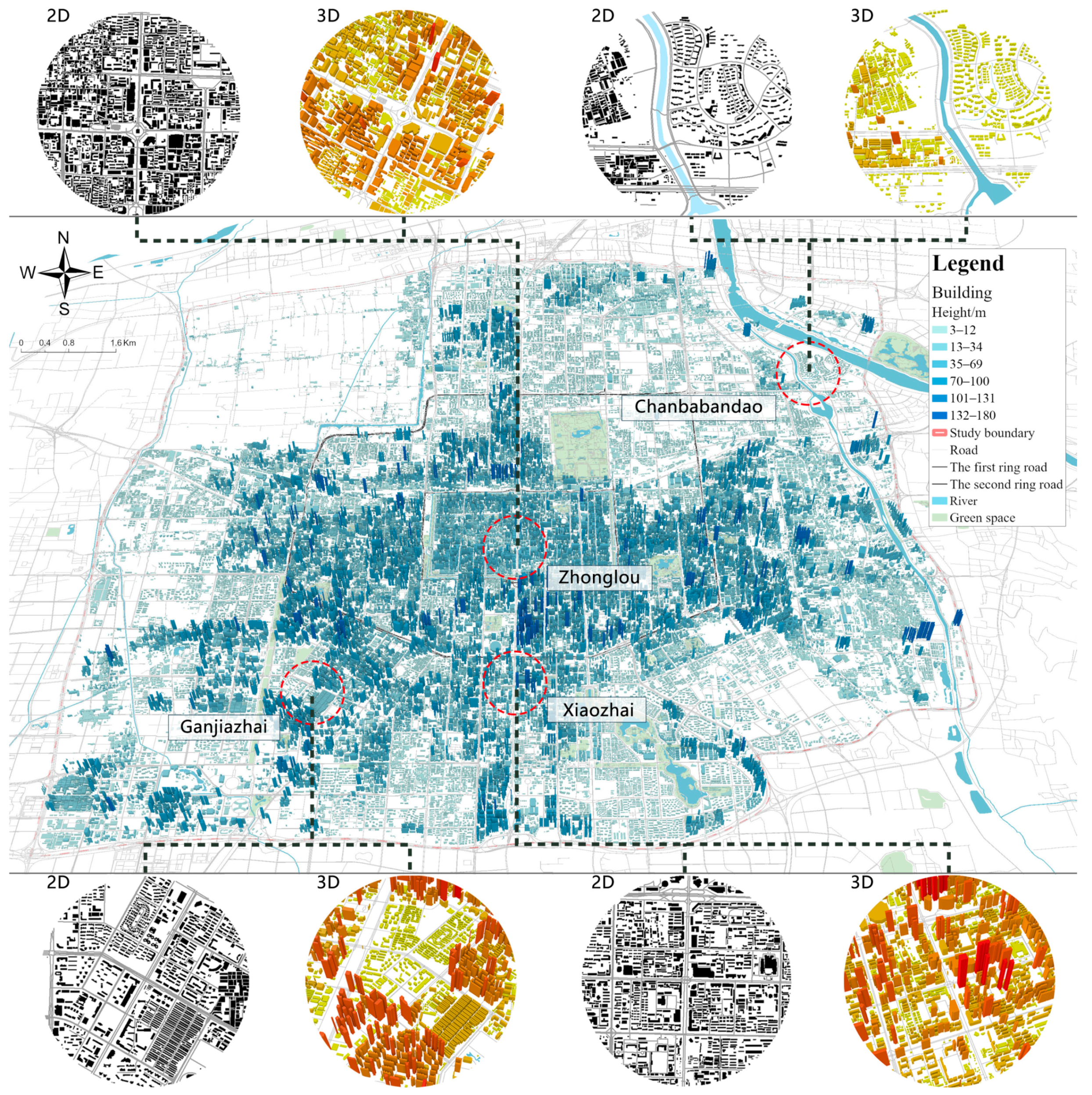
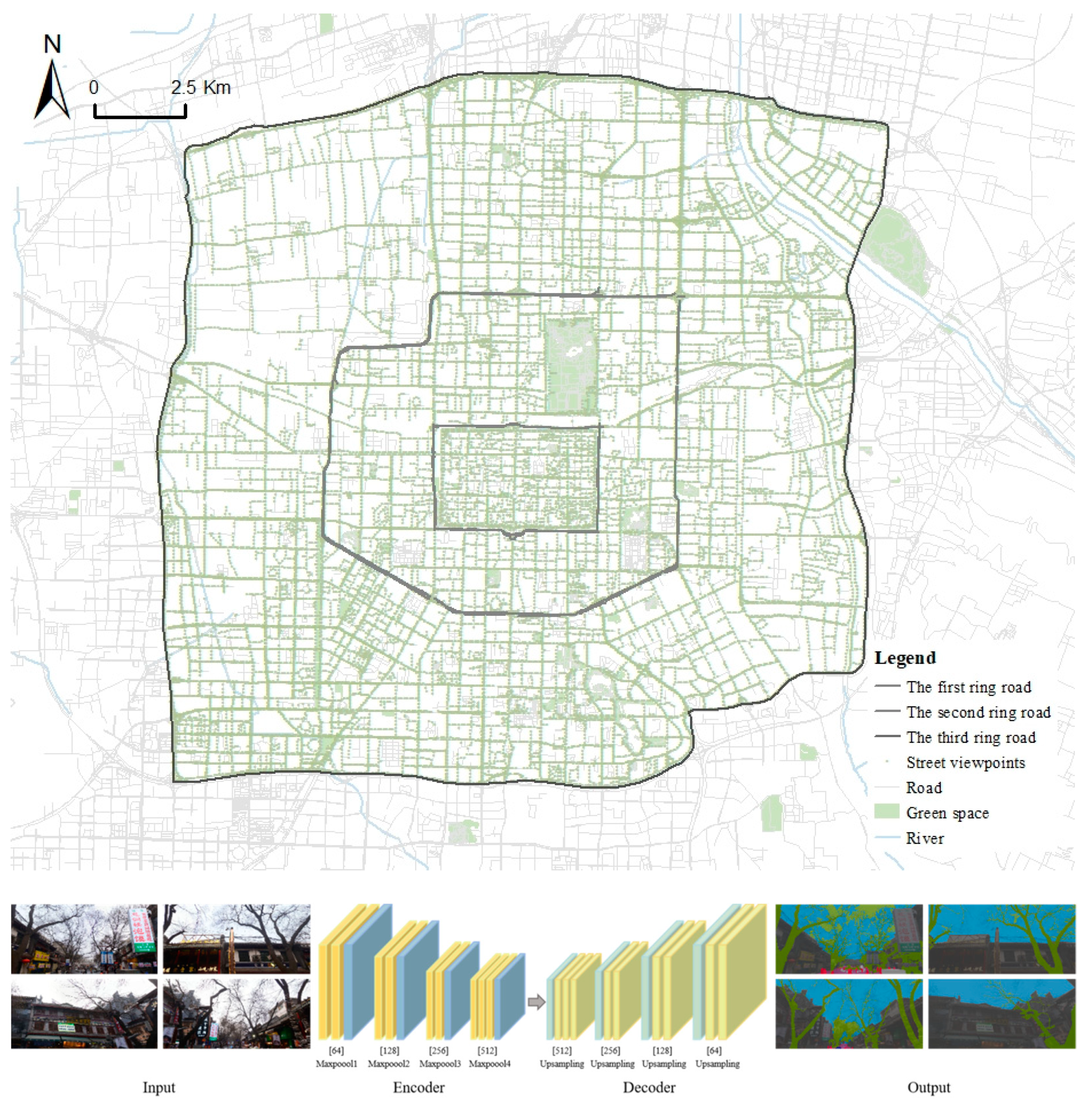
2.1. Study Area
2.2. Data Sources
2.2.1. Baidu Heat Map
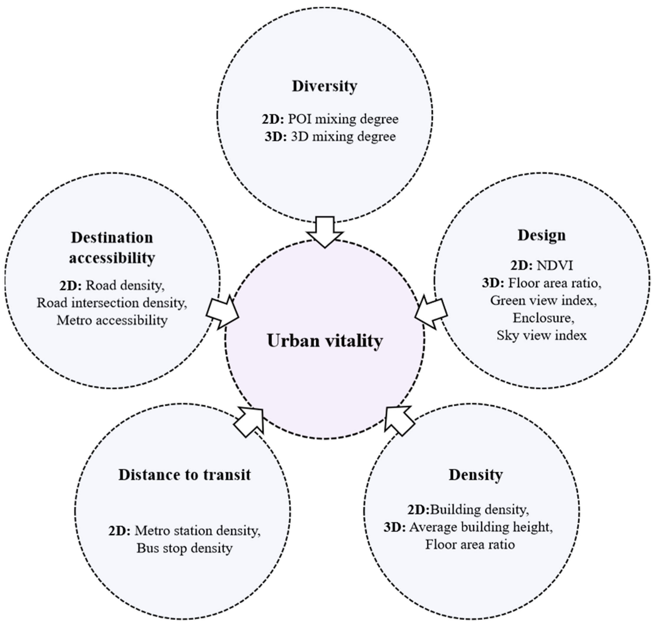
2.2.2. Variables
- (1)
- POI mixing degree
- (2)
- Street view images
2.3. Methodology
3. Results
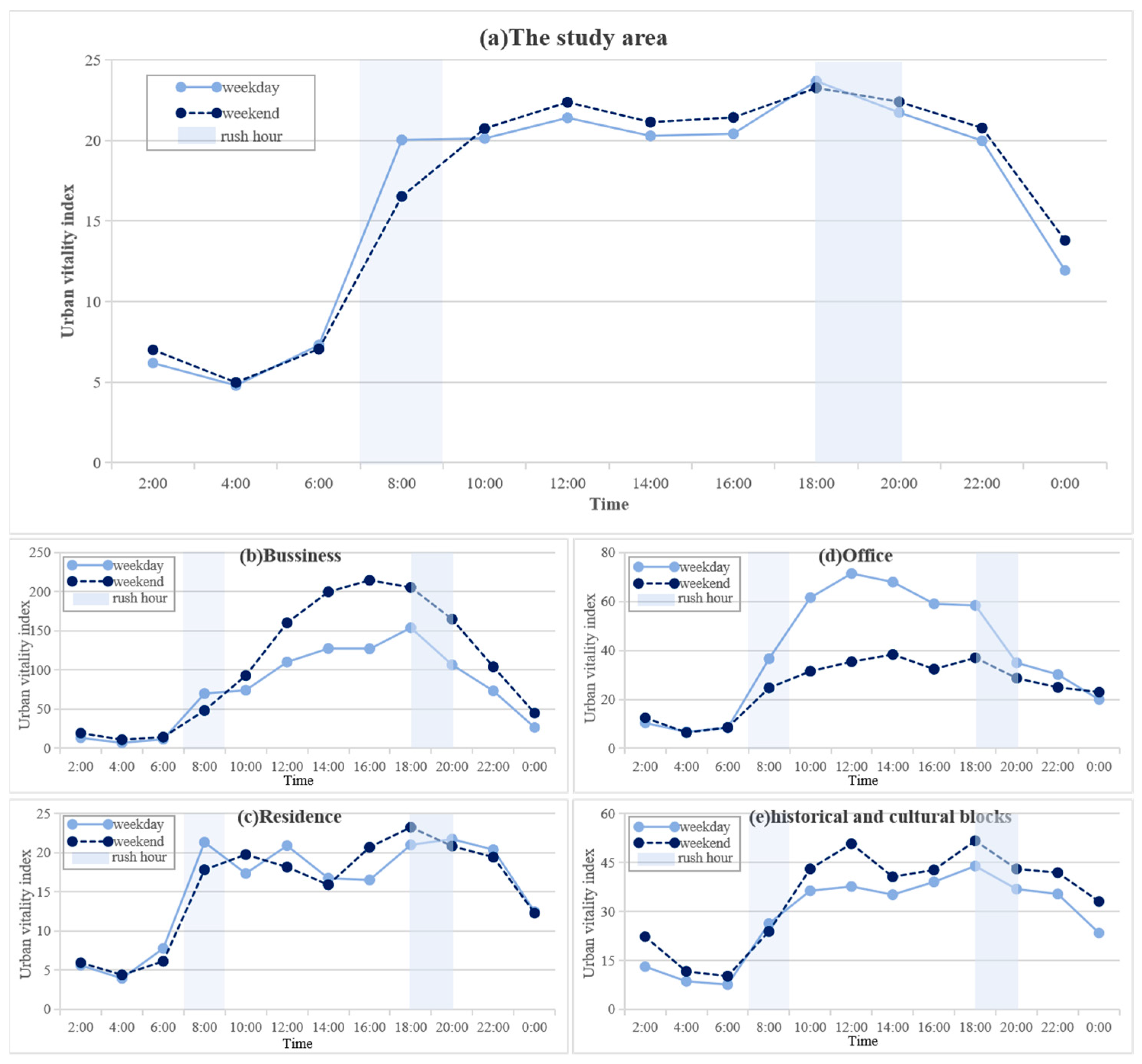
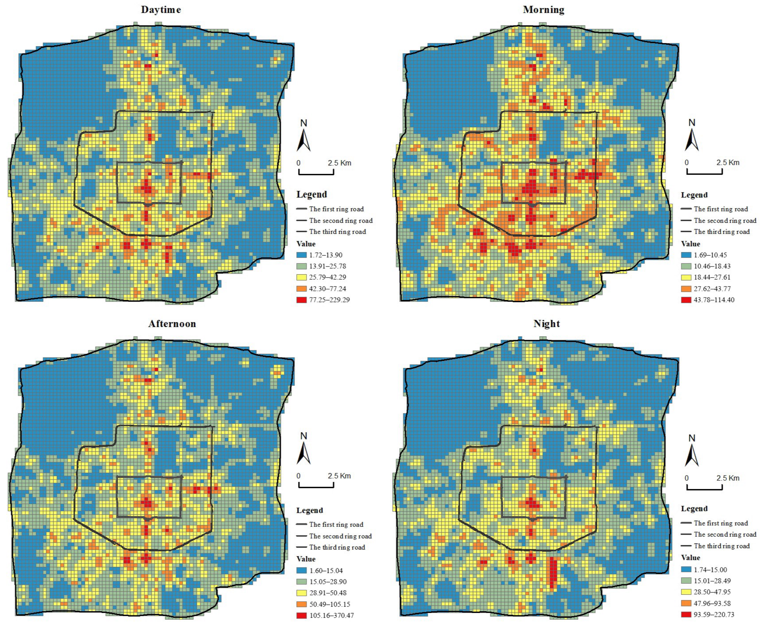
3.1. Spatial–Temporal Variations in Urban Vitality
3.2. Spatial Autocorrelation Analysis of Urban Vitality
3.3. Results of the OLS and GWR Models
3.3.1. OLS Model Results
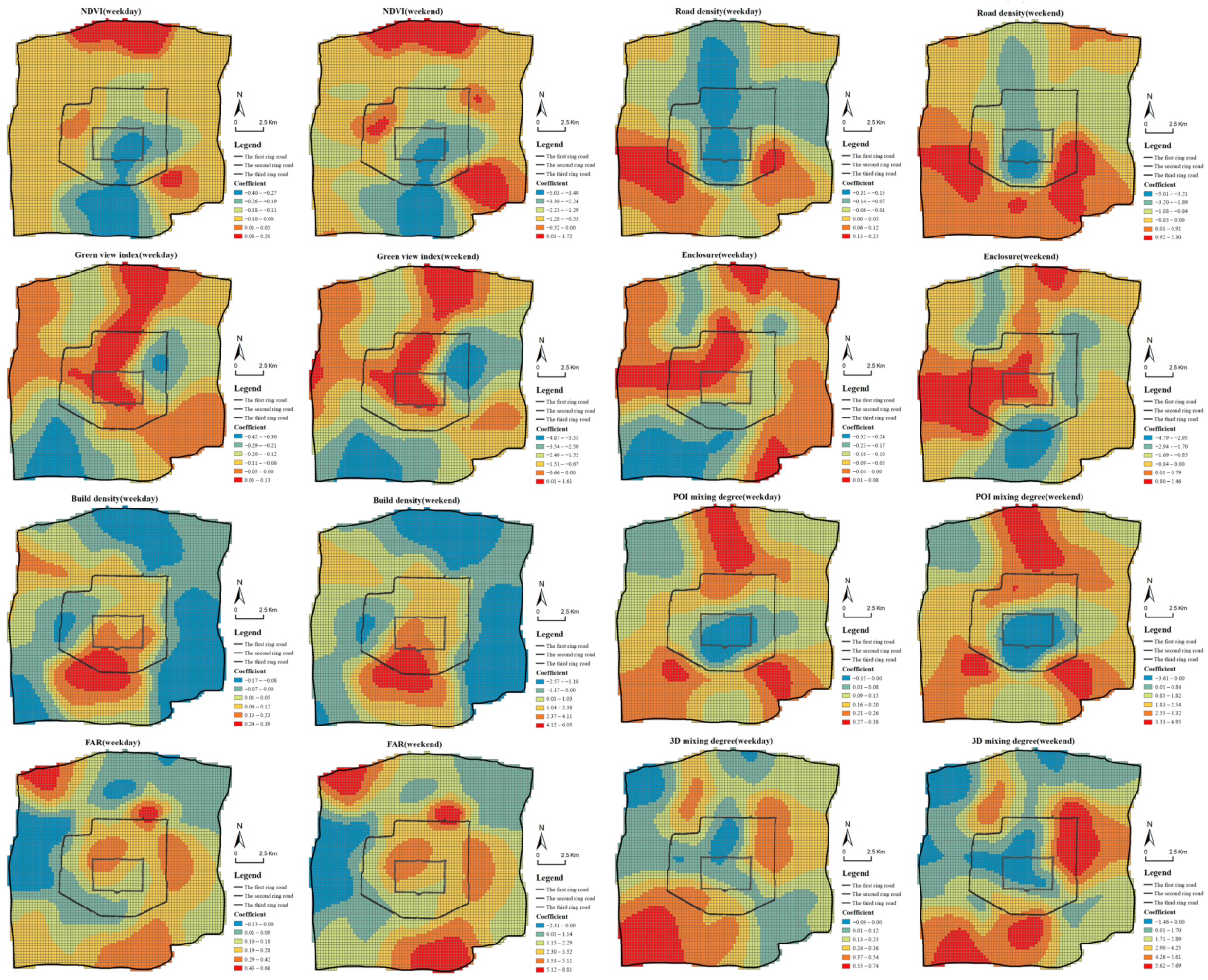
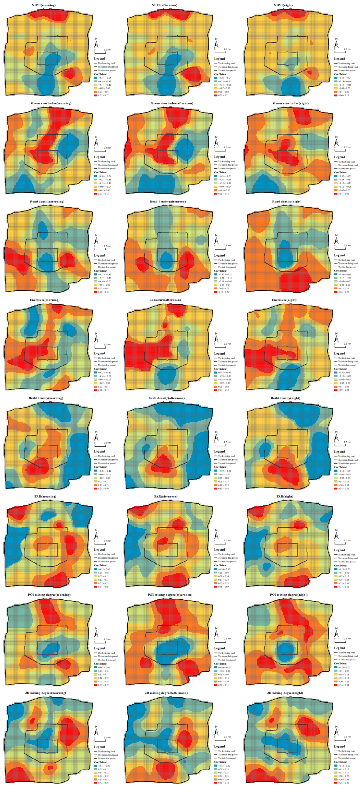
3.3.2. GWR Model Results
4. Discussion
4.1. Green Space: NDVI and Green View Index
4.2. Road Space: Road Density and Enclosure
4.3. Building Space: Building Density and FAR
4.4. Mixed Function: POI Mixing Degree and 3D Mixing Degree
5. Conclusions
Author Contributions
Funding
Data Availability Statement
Acknowledgments
Conflicts of Interest
Abbreviations
Appendix A
References
- Wu, C.; Ye, Y.; Gao, F.; Ye, X. Using Street View Images to Examine the Association Between Human Perceptions of Locale and Urban Vitality in Shenzhen, China. Sustain. Cities Soc. 2023, 88, 104291. [Google Scholar] [CrossRef]
- Wu, W.; Dang, Y.; Zhao, K.; Chen, Z.; Niu, X. Spatial Nonlinear Effects of Urban Vitality Under the constraints of Development Intensity and Functional Diversity. Alex. Eng. J. 2023, 77, 645–656. [Google Scholar] [CrossRef]
- Liu, W. Spatial Impact of the Built Environment on Street Vitality: A Case Study of the Tianhe District, Guangzhou. Front. Environ. Sci. 2022, 10, 966562. [Google Scholar]
- Lv, G.; Zheng, S.; Hu, W. Exploring the Relationship Between the Built Environment and Block Vitality Based on Multi-source Big Data: An Analysis in Shenzhen, China. Geomat. Nat. Hazards Risk 2022, 13, 1593–1613. [Google Scholar] [CrossRef]
- Lin, J.; Zhuang, Y.; Zhao, Y.; Li, H.; He, X.; Lu, S. Measuring the Non-linear Relationship Between Three-dimensional Built Environment and Urban Vitality Based on a Random Forest Model. Int. J. Environ. Res. Public Health 2023, 20, 734. [Google Scholar] [CrossRef] [PubMed]
- Lu, S.; Shi, C.; Yang, X. Impacts of Built Environment on Urban Vitality: Regression Analyses of Beijing and Chengdu, China. Int. J. Environ. Res. Public Health 2019, 16, 4592. [Google Scholar] [CrossRef] [PubMed]
- Liu, S.; Zhang, L.; Long, Y.; Long, Y.; Xu, M. A new urban vitality analysis and evaluation framework based on Human Activity Modeling Using Multi-source Big Data. Isprs Int. J. Geo-Inf. 2020, 9, 617. [Google Scholar] [CrossRef]
- Xu, X.; Xu, X.; Guan, P.; Ren, Y.; Wang, W.; Xu, N. The Cause and Evolution of Urban Street Vitality Under the Time Dimension: Nine Cases of Streets in Nanjing City, China. Sustainability 2018, 10, 2797. [Google Scholar] [CrossRef]
- Ye, Y.; Li, D.; Liu, X. How Block Density and Typology Affect Urban Vitality: An Exploratory Analysis in Shenzhen, China. Urban Geogr. 2018, 39, 631–652. [Google Scholar] [CrossRef]
- Lu, Y.; Sarkar, C.; Xiao, Y. The Effect of Street-Level Greenery on Walking Behavior: Evidence from Hong Kong. Soc. Sci. Med. 2018, 208, 41–49. [Google Scholar] [CrossRef]
- Luo, P.Y.; Yu, B.J.; Li, P.F.; Liang, P. Spatially varying Impacts of the Built Environment on Physical Activity from a Human-scale View: Using Street View Data. Front. Environ. Sci. 2022, 10, 1021081. [Google Scholar] [CrossRef]
- Jacobs, J.M. The Death and Life of Great American Cities; Random House: New York, NY, USA, 1962. [Google Scholar]
- Lynch, K.M. Good City Form; MIT Press: Cambridge, MA, USA, 1984. [Google Scholar]
- Kang, C.-D. Effects of the Human and Built Environment on Neighborhood Vitality: Evidence from Seoul, Korea, Using Mobile Phone Data. J. Urban Plan. Dev. 2020, 146, 05020024. [Google Scholar] [CrossRef]
- Wu, W.; Niu, X. Influence of Built Environment on Urban Vitality: Case Study of Shanghai Using Mobile Phone Location Data. J. Urban Plan. Dev. 2019, 145, 04019007. [Google Scholar] [CrossRef]
- Lu, S.; Huang, Y.; Shi, C.; Yang, X. Exploring the Associations Between Urban Form and Neighborhood Vibrancy: A Case Study of Chengdu, China. Isprs Int. J. Geo-Inf. 2019, 8, 165. [Google Scholar] [CrossRef]
- Wang, B.; Lei, Y.; Xue, D.; Liu, J.; Wei, C. Elaborating Spatiotemporal Associations Between the Built Environment and Urban Vibrancy: A Case of Guangzhou City, China. Chin. Geogr. Sci. 2022, 32, 480–492. [Google Scholar] [CrossRef]
- Yang, Y.; Ma, Y.; Jiao, H. Exploring the Correlation Between Block Vitality and Block Environment Based on Multisource Big Data: Taking Wuhan City as an Example. Land 2021, 10, 984. [Google Scholar] [CrossRef]
- Shi, Y.; Yang, J.; Shen, P. Revealing the Correlation Between Population Density and the spatial distribution of Urban Public Service Facilities with Mobile Phone Data. Isprs Int. J. Geo-Inf. 2020, 9, 38. [Google Scholar] [CrossRef]
- Cervero, R.; Kockelman, K.M. Travel Demand and the 3Ds: Density, Diversity, and Design. Transp. Res. Part D-Transp. Environ. 1997, 2, 199–219. [Google Scholar] [CrossRef]
- Chen, L.; Zhao, L.; Xiao, Y.; Lu, Y. Investigating the spatiotemporal pattern between the built environment and Urban Vibrancy Using Big Data in Shenzhen, China. Comput. Environ. Urban Syst. 2022, 95, 101827. [Google Scholar] [CrossRef]
- Xiao, L.; Liu, J. Exploring Non-Linear Built Environment Effects on Urban Vibrancy Under COVID-19: The Case of Hong Kong. Appl. Geogr. 2023, 155, 102960. [Google Scholar] [CrossRef]
- Li, X.J.; Zhang, C.R.; Li, W.D.; Ricard, R.; Meng, Q.; Zhang, W. Assessing street-level urban greenery using Google Street View and a modified green view index. Urban For. Urban Green. 2015, 14, 675–685. [Google Scholar] [CrossRef]
- Kang, J.; Körner, M.; Wang, Y.; Taubenböck, H.; Zhu, X.X. Building instance classification using street view images. Isprs J. Photogramm. Remote Sens. 2018, 145, 44–59. [Google Scholar] [CrossRef]
- Liu, L.; Silva, E.A.; Wu, C.; Wang, H. Amachine learning-based method for the large-scale evaluation of the qualities of the urban environment. Comput. Environ. Urban Syst. 2017, 65, 113–125. [Google Scholar] [CrossRef]
- Zhang, F.; Zhou, B.; Liu, L.; Liu, Y.; Fung, H.H.; Lin, H.; Ratti, C. Measuring human perceptions of a large-scale urban region using machine learning. Landsc. Urban Plan. 2018, 180, 148–160. [Google Scholar] [CrossRef]
- Gao, M.; Fang, C.Y. Deciphering urban cycling: Analyzing the nonlinear impact of street environments on cycling volume using crowdsourced tracker data and machine learning. J. Transp. Geogr. 2025, 124, 104179. [Google Scholar] [CrossRef]
- Liu, J.X.; Chau, K.W.; Bao, Z.K. Multiscale spatial analysis of metro usage and its determinants for Sustainable Urban Development in Shenzhen, China. Tunn. Undergr. Space Technol. 2023, 133, 104912. [Google Scholar] [CrossRef]
- Tu, W.; Zhu, T.; Zhong, C.; Zhang, X.; Xu, Y.; Li, Q. Exploring Metro Vibrancy and its Relationship with Built Environment: A Cross-city Comparison Using Multi-source Urban Data. Geo-Spat. Inf. Sci. 2022, 25, 182–196. [Google Scholar] [CrossRef]
- Lyu, F.; Zhang, L. Using Multi-source Big Data to Understand the Factors Affecting Urban Park Use in Wuhan. Urban For. Urban Green. 2019, 43, 126367. [Google Scholar] [CrossRef]
- Song, Y.; Lyu, Y.; Qian, S.; Zhang, X.; Lin, H.; Wang, S. Identifying Urban Candidate Brownfield Sites Using Multi-source Data: The Case of Changchun City, China. Land Use Policy 2022, 117, 106084. [Google Scholar] [CrossRef]
- Luo, P.Y.; Yu, B.J.; Li, P.F.; Liang, P.; Zhang, Q.; Yang, L. Understanding the Relationship Between 2D/3D Variables and Land Surface Temperature in Plain and Mountainous Cities: Relative Importance and Interaction Effects. Build. Environ. 2023, 245, 110959. [Google Scholar] [CrossRef]
- Yang, L.C.; Ao, Y.B.; Ke, J.T.; Lu, Y.; Liang, Y. To Walk or Not to Walk? Examining Non-linear Effects of streetscape greenery on Walking Propensity of Older Adults. J. Transp. Geogr. 2021, 94, 103099. [Google Scholar] [CrossRef]
- Luo, P.Y.; Yu, B.J.; Li, P.F.; Liang, P.; Liang, Y.; Yang, L. How 2D and 3D Built Environments Impact Urban Surface Temperature Under Extreme Heat: A Study in Chengdu, China. Build. Environ. 2023, 231, 110035. [Google Scholar] [CrossRef]
- Gao, J.B.; Li, S.C. Detecting Spatially Non-Stationary and Scale-dependent Relationships Between Urban Landscape Fragmentation and Related Factors Using Geographically Weighted Regression. Appl. Geogr. 2011, 31, 292–302. [Google Scholar] [CrossRef]
- Gao, Y.J.; Zhao, J.Y.; Han, L. Exploring the Spatial Heterogeneity of Urban Heat Island Effect and its Relationship to Block Morphology with the Geographically Weighted Regression Model. Sustain. Cities Soc. 2022, 76, 103431. [Google Scholar] [CrossRef]
- Li, S.Y.; Lyu, D.J.; Huang, G.P.; Zhang, X.; Gao, F.; Chen, Y.; Liu, X. Spatially Varying Impacts of Built Environment Factors on Rail Transit Ridership at Station Level: A Case Study in Guangzhou, China. J. Transp. Geogr. 2020, 82, 102631. [Google Scholar] [CrossRef]
- Wang, S.J.; Shi, C.Y.; Fang, C.L.; Feng, K. Examining the Spatial Variations of Determinants of Energy-related CO2 Emissions in China at the City Level Using Geographically Weighted Regression Model. Appl. Energy 2019, 235, 95–105. [Google Scholar] [CrossRef]
- Li, J.; Li, J.; Yuan, Y.; Li, G. Spatiotemporal Distribution Characteristics and Mechanism Analysis of Urban Population Density: A Case of Xi’an, Shaanxi, China. Cities 2019, 86, 62–70. [Google Scholar] [CrossRef]
- Yang, J.; Cao, J.; Zhou, Y. Elaborating Non-linear Associations and Synergies of Subway Access and Land Uses with Urban Vitality in Shenzhen. Transp. Res. Part A-Policy Pract. 2021, 144, 74–88. [Google Scholar] [CrossRef]
- Yang, X.P.; Zhao, Z.Y.; Shi, C.Y.; Luo, L.; Tu, W. The Dynamic Heterogeneous Relationship Between Urban Population Distribution and Built Environment in Xi’an, China: A Case Study. Remote Sens. 2023, 15, 2257. [Google Scholar] [CrossRef]
- Yang, L.; Lu, Y.; Cao, M.; Wang, R.; Chen, J. Assessing Accessibility to Peri-urban Parks Considering Supply, Demand, and Traffic Conditions. Landsc. Urban Plan. 2025, 257, 105313. [Google Scholar] [CrossRef]
- Li, M.Y.; Liu, J.X.; Lin, Y.F.; Xiao, L.; Zhou, J. Revitalizing Historic Districts: Identifying Built Environment Predictors for Street Vibrancy Based on Urban Sensor Data. Cities 2021, 117, 103305. [Google Scholar] [CrossRef]
- Lin, J.Y.; Wan, H.Y.; Cui, Y.T. Analyzing the Spatial Factors Related to the Distributions of Building Heights in Urban Areas: A Comparative Case Study in Guangzhou and Shenzhen. Sustain. Cities Soc. 2020, 52, 101854. [Google Scholar] [CrossRef]
- Xu, G.; Su, J.; Xia, C.; Li, X.; Xiao, R. Spatial Mismatches Between Nighttime Light Intensity and Building Morphology in Shanghai, China. Sustain. Cities Soc. 2022, 81, 103851. [Google Scholar] [CrossRef]
- Jiang, Y.; Liu, D.; Ren, L.; Grekousis, G.; Lu, Y. Tree Abundance, Species Richness, or species mix? Exploring the Relationship Between Features of Urban Street Trees and Pedestrian Volume in Jinan, China. Urban For. Urban Green. 2024, 95, 128294. [Google Scholar] [CrossRef]


| Variables (Unit) | Abbreviations | Std | Mean | Min | Max |
|---|---|---|---|---|---|
| 2D variables | |||||
| POI mixing degree | POI_MD | 0.761 | 1.553 | 0 | 2.622 |
| Normalized difference vegetation index | NDVI | 0.063 | 0.346 | 0.040 | 0.638 |
| Building density | BD | 0.142 | 0.183 | 0 | 0.853 |
| Road density (km/km2) | RD | 5.408 | 7.345 | 0 | 44.710 |
| Road intersection density (1/62,500 m2) | RID | 4.596 | 2.759 | 0 | 62 |
| Metro station density (1/62,500 m2) | MSD | 0.171 | 0.026 | 0 | 2 |
| Bus stop density (1/62,500 m2) | BSD | 5.110 | 2.472 | 0 | 43 |
| Metro accessibility (m) | SA | 1058.118 | 1066.778 | 7.498 | 6530.163 |
| 3D variables | |||||
| Average building height (m) | ABH | 11.939 | 12.497 | 0 | 120 |
| Floor area ratio | FAR | 1.335 | 1.070 | 0 | 8.748 |
| Green view index | GVI | 0.132 | 0.169 | 0 | 0.744 |
| Enclosure | EN | 0.153 | 0.195 | 0 | 0.867 |
| Sky view index | SVI | 0.102 | 0.126 | 0 | 0.470 |
| 3D mixing degree | 3D_MD | 0.639 | 1.338 | 0 | 2.094 |
| Period | Weekday | Weekend | ||||
|---|---|---|---|---|---|---|
| Moran’s I | z-Score | p-Value | Moran’s I | z-Score | p-Value | |
| Morning | 0.823 | 124.801 | 0.001 | 0.817 | 124.149 | 0.001 |
| Afternoon | 0.788 | 119.376 | 0.001 | 0.690 | 105.631 | 0.001 |
| night | 0.822 | 127.195 | 0.001 | 0.756 | 117.117 | 0.001 |
| Variable | Weekday | Weekend | ||||
|---|---|---|---|---|---|---|
| Morning | Afternoon | Night | MORNING | afternoon | Night | |
| POI_MD | 0.210 *** | 0.181 *** | 0.245 *** | 0.221 *** | 0.156 *** | 0.210 *** |
| (0.013) | (0.013) | (0.013) | (0.013) | (0.014) | (0.014) | |
| NDVI | −0.092 *** | −0.083 *** | −0.068 *** | −0.097 *** | −0.078 *** | −0.065 *** |
| (0.010) | (0.011) | (0.010) | (0.010) | (0.011) | (0.011) | |
| BD | −0.062 *** | −0.061 *** | −0.042 ** | −0.058 *** | −0.066 *** | −0.033 * |
| (0.014) | (0.015) | (0.015) | (0.014) | (0.016) | (0.016) | |
| RD | 0.000 | 0.021 | 0.031 * | −0.031 * | −0.006 | 0.031 * |
| (0.013) | (0.014) | (0.014) | (0.013) | (0.015) | (0.015) | |
| RID | 0.104 *** | 0.104 *** | 0.076 *** | 0.122 *** | 0.127 *** | 0.090 *** |
| (0.013) | (0.013) | (0.013) | (0.013) | (0.014) | (0.014) | |
| MSD | 0.102 *** | 0.115 *** | 0.074 *** | 0.093 *** | 0.138 *** | 0.098 *** |
| (0.010) | (0.010) | (0.010) | (0.010) | (0.011) | (0.011) | |
| BSD | 0.123 *** | 0.125 *** | 0.090 *** | 0.117 *** | 0.122 *** | 0.089 *** |
| (0.010) | (0.011) | (0.011) | (0.010) | (0.011) | (0.011) | |
| SA | −0.189 *** | −0.158 *** | −0.174 *** | −0.201 *** | −0.162 *** | −0.153 *** |
| (0.011) | (0.012) | (0.011) | (0.011) | (0.012) | (0.012) | |
| ABH | 0.001 | −0.013 | −0.026 | −0.036 * | −0.061 *** | −0.051 ** |
| (0.016) | (0.017) | (0.017) | (0.016) | (0.018) | (0.018) | |
| FAR | 0.311 *** | 0.336 *** | 0.272 *** | 0.314 *** | 0.335 *** | 0.276 *** |
| (0.019) | (0.020) | (0.020) | (0.019) | (0.021) | (0.021) | |
| GVI | −0.105 *** | −0.112 *** | −0.128 *** | −0.115 *** | −0.116 *** | −0.121 *** |
| (0.021) | (0.022) | (0.022) | (0.021) | (0.023) | (0.023) | |
| EN | −0.114 *** | −0.144 *** | −0.071 ** | −0.049 * | −0.087 ** | −0.063 * |
| (0.025) | (0.026) | (0.026) | (0.024) | (0.027) | (0.027) | |
| SVI | −0.226 *** | −0.222 *** | −0.268 *** | −0.229 *** | −0.178 *** | −0.221 *** |
| (0.022) | (0.023) | (0.022) | (0.021) | (0.024) | (0.024) | |
| 3D_MD | 0.267 *** | 0.284 *** | 0.261 *** | 0.248 *** | 0.237 *** | 0.228 *** |
| (0.039) | (0.041) | (0.040) | (0.039) | (0.043) | (0.043) | |
| R2 | 0.496 | 0.454 | 0.467 | 0.510 | 0.388 | 0.389 |
| Diagnostic Index | Weekday | Weekend | ||||||
|---|---|---|---|---|---|---|---|---|
| Morning | Afternoon | Night | All Day | Morning | Afternoon | Night | All Day | |
| Residual Squares | 1799.985 | 1993.542 | 2048.099 | 1803.190 | 1795.147 | 2452.490 | 2495.854 | 425,039.370 |
| AICc | 10,082.584 | 10,667.611 | 10,822.261 | 10,092.771 | 10,067.166 | 11,854.398 | 11,954.794 | 41,382.685 |
| R2 | 0.686 | 0.652 | 0.642 | 0.685 | 0.686 | 0.572 | 0.564 | 0.626 |
| Adjusted R2 | 0.669 | 0.633 | 0.623 | 0.668 | 0.670 | 0.549 | 0.541 | 0.606 |
| Bandwidth | 955.844 | 955.844 | 955.844 | 955.844 | 955.844 | 955.844 | 955.844 | 955.844 |
| Variable | Weekday | Weekend | ||||||||||||||
|---|---|---|---|---|---|---|---|---|---|---|---|---|---|---|---|---|
| Morning | Afternoon | Night | All Day | Morning | Afternoon | Night | All Day | |||||||||
| Mean | STD | Mean | STD | Mean | STD | Mean | STD | Mean | STD | Mean | STD | Mean | STD | Mean | STD | |
| POI_MD | 0.151 | 0.079 | 0.119 | 0.098 | 0.187 | 0.082 | 0.153 | 0.085 | 0.167 | 0.078 | 0.097 | 0.112 | 0.162 | 0.083 | 1.999 | 1.271 |
| NDVI | −0.095 | 0.116 | −0.089 | 0.113 | −0.084 | 0.092 | −0.092 | 0.108 | −0.100 | 0.097 | −0.084 | 0.089 | −0.080 | 0.073 | −1.268 | 1.224 |
| BD | −0.004 | 0.100 | 0.005 | 0.103 | 0.024 | 0.142 | 0.008 | 0.112 | 0.009 | 0.120 | 0.012 | 0.123 | 0.040 | 0.148 | 0.287 | 1.822 |
| RD | −0.034 | 0.095 | −0.019 | 0.100 | −0.006 | 0.103 | −0.021 | 0.098 | −0.054 | 0.081 | −0.033 | 0.089 | −0.003 | 0.114 | −0.435 | 1.250 |
| RID | 0.103 | 0.055 | 0.101 | 0.060 | 0.065 | 0.070 | 0.074 | 0.056 | 0.119 | 0.066 | 0.117 | 0.079 | 0.076 | 0.082 | 1.236 | 0.797 |
| MSD | 0.074 | 0.058 | 0.081 | 0.061 | 0.057 | 0.045 | 0.100 | 0.065 | 0.069 | 0.052 | 0.103 | 0.061 | 0.075 | 0.053 | 1.417 | 0.819 |
| BSD | 0.103 | 0.065 | 0.106 | 0.066 | 0.077 | 0.059 | 0.094 | 0.061 | 0.102 | 0.060 | 0.108 | 0.057 | 0.079 | 0.055 | 1.527 | 1.078 |
| SA | −0.586 | 0.492 | −0.600 | 0.547 | −0.415 | 0.401 | −0.560 | 0.495 | −0.526 | 0.487 | −0.588 | 0.616 | −0.421 | 0.448 | −7.578 | 7.609 |
| ABH | 0.067 | 0.099 | 0.052 | 0.094 | 0.039 | 0.081 | 0.055 | 0.091 | 0.049 | 0.084 | 0.023 | 0.079 | 0.019 | 0.084 | 0.427 | 1.143 |
| FAR | 0.146 | 0.132 | 0.172 | 0.128 | 0.134 | 0.137 | 0.157 | 0.132 | 0.137 | 0.142 | 0.169 | 0.124 | 0.140 | 0.124 | 2.203 | 1.808 |
| GVI | −0.097 | 0.112 | −0.104 | 0.121 | −0.101 | 0.089 | −0.104 | 0.110 | −0.100 | 0.097 | −0.106 | 0.111 | −0.093 | 0.083 | −1.462 | 1.358 |
| EN | −0.095 | 0.097 | −0.117 | 0.115 | −0.033 | 0.074 | −0.089 | 0.090 | −0.034 | 0.078 | −0.067 | 0.104 | −0.023 | 0.086 | −0.646 | 1.244 |
| SVI | −0.183 | 0.148 | −0.169 | 0.168 | −0.193 | 0.140 | −0.186 | 0.152 | −0.177 | 0.145 | −0.118 | 0.157 | −0.140 | 0.154 | −2.063 | 2.129 |
| 3D_MD | 0.234 | 0.190 | 0.245 | 0.222 | 0.192 | 0.131 | 0.233 | 0.183 | 0.204 | 0.151 | 0.194 | 0.180 | 0.154 | 0.120 | 2.686 | 2.101 |
Disclaimer/Publisher’s Note: The statements, opinions and data contained in all publications are solely those of the individual author(s) and contributor(s) and not of MDPI and/or the editor(s). MDPI and/or the editor(s) disclaim responsibility for any injury to people or property resulting from any ideas, methods, instructions or products referred to in the content. |
© 2025 by the authors. Licensee MDPI, Basel, Switzerland. This article is an open access article distributed under the terms and conditions of the Creative Commons Attribution (CC BY) license (https://creativecommons.org/licenses/by/4.0/).
Share and Cite
Peng, Y.; Cui, X.; Yu, B.; Liu, R.; Li, H. How 2D and 3D Built Environment Impact Urban Vitality: Evidence from Overhead-Level to Eye-Level Urban Form Metrics. Land 2025, 14, 1026. https://doi.org/10.3390/land14051026
Peng Y, Cui X, Yu B, Liu R, Li H. How 2D and 3D Built Environment Impact Urban Vitality: Evidence from Overhead-Level to Eye-Level Urban Form Metrics. Land. 2025; 14(5):1026. https://doi.org/10.3390/land14051026
Chicago/Turabian StylePeng, Yi, Xu Cui, Bingjie Yu, Runze Liu, and Hong Li. 2025. "How 2D and 3D Built Environment Impact Urban Vitality: Evidence from Overhead-Level to Eye-Level Urban Form Metrics" Land 14, no. 5: 1026. https://doi.org/10.3390/land14051026
APA StylePeng, Y., Cui, X., Yu, B., Liu, R., & Li, H. (2025). How 2D and 3D Built Environment Impact Urban Vitality: Evidence from Overhead-Level to Eye-Level Urban Form Metrics. Land, 14(5), 1026. https://doi.org/10.3390/land14051026