Article

Land Development 1985–2023 as a Function of Road Improvement, Employment, and Mobility: A Case Study of Tennessee

by
Jayanta Biswas
* and
Anzhelika Antipova
Department of Earth Sciences, University of Memphis, Memphis, TN 38152, USA
*
Author to whom correspondence should be addressed.
Land 2025, 14(5), 1025; https://doi.org/10.3390/land14051025
Submission received: 29 March 2025 / Revised: 3 May 2025 / Accepted: 6 May 2025 / Published: 8 May 2025

Abstract

:
Metaverse environments aim at replicating physical reality at various scales. While the potential growth of digital land is limitless, certain development factors may drive greater growth and lead to changes in surrounding land use and the expansion of developed land. In this study, we are bridging digital and physical world living environments using physical land as an example. Specifically, we focus on Tennessee as a study area and offer a spatial perspective on factors of urban land growth and study the relationship between infrastructure (road) development, employment, mobility, and land use change in the physical world, which may help understand this connection in the digital land and real estate domain. We show a significant role of employment hubs in driving developed land growth (i.e., land development). Economic activity consistently appears significant in urban land expansion, with the land development effect of employment stretching over a larger area well beyond immediate proximity to road infrastructure. Land development is measured in this study by a developed land density in both urban and rural areas. Mobility (measured by VMT) has a weaker impact on land development though still positive and statistically significant. This research is crucial for developing sustainable land growth strategies and informing future transport planning and land-use policies.

1. Introduction

Despite significant differences between physical and digital land, we can think of similarities in terms of their use and valuation. One can find parallels between physical and digital land as follows. Improvement of and better accessibility to physical land’s infrastructure, including roads, increases physical land’s property values. Similar principles apply to real estate in the metaverse. The value of digital land may increase with improvements in digital infrastructure, such as virtual pathways, digital accessibility to services, and virtual connectivity between spaces in the metaverse. Further, various factors, including demographics, economic growth, and infrastructure development, all shape real estate investment in physical land, while the growth of the metaverse, among other factors, influences real estate investments in digital land. Understanding these parallels enables one to see how virtual real estate can grow and evolve.
Much like physical land, digital land and real estate can grow. It is important to determine what factors are more important in driving growth. Since digital plots can represent offices and entertainment (and thus, jobs), what is the role of employment as virtual land expands? Without the constraints of physicality, will the changes in land use, such as digital infrastructure improvement, alter digital land and real estate in the metaverse?
In order for future City- and metaverse environments to successfully replicate physical reality at various scales, one must understand what factors may potentially drive the growth of the physical-world developed land. We need to better understand the linkage between development-caused factors, such as increased employment, greater vehicle traffic, and changes in surrounding land use. In this study, we are using the physical land as an example. Specifically, we offer a spatial perspective on factors of urban land growth, including employment and road improvement. Here, we study the relationship between infrastructure (road) development, employment, amount of travel, and land use change in the physical world, which may help us understand this connection in the digital land and real estate domain.
In the physical world, the transportation network is the backbone of social development and land use expansion [1,2,3]. Transportation systems and land use co-exist and influence the landform. So, any land-use changes alter travel behavior and demand, influencing vehicle flows and road infrastructure. Furthermore, vehicle flows drive the construction and improvement of road network facilities. Finally, improved and new transportation infrastructure enhances accessibility and mobility patterns, leading to the relocation of socioeconomic activities and land use [4,5]. Most of the time, the governments take different public policies to road improvements and development to support integration, connect various functional areas and administrative regions, aggregation of logistics, energy, information, capital, and other flows [6]. For example, in the USA, the Interstate Highway System, a network of controlled-access highways that forms a part of the National Highway System of the United States, was introduced to support national security and facilitate interstate travel and commerce [7]. Although road construction and improvement, which includes activities such as widening, resurfacing, and adding new lanes or features to existing roads, can be carried out for several purposes, they can also lead to economic development [8,9,10,11]. Diaconu et al. [12] observed that new highway infrastructure in Romania led to substantial land use change, replacing agricultural land with industrial and built-up areas. Similarly, Aïkous et al. [13] demonstrated that highway expansion in Montreal significantly increased the probability of industrial and commercial construction near a new access ramp.
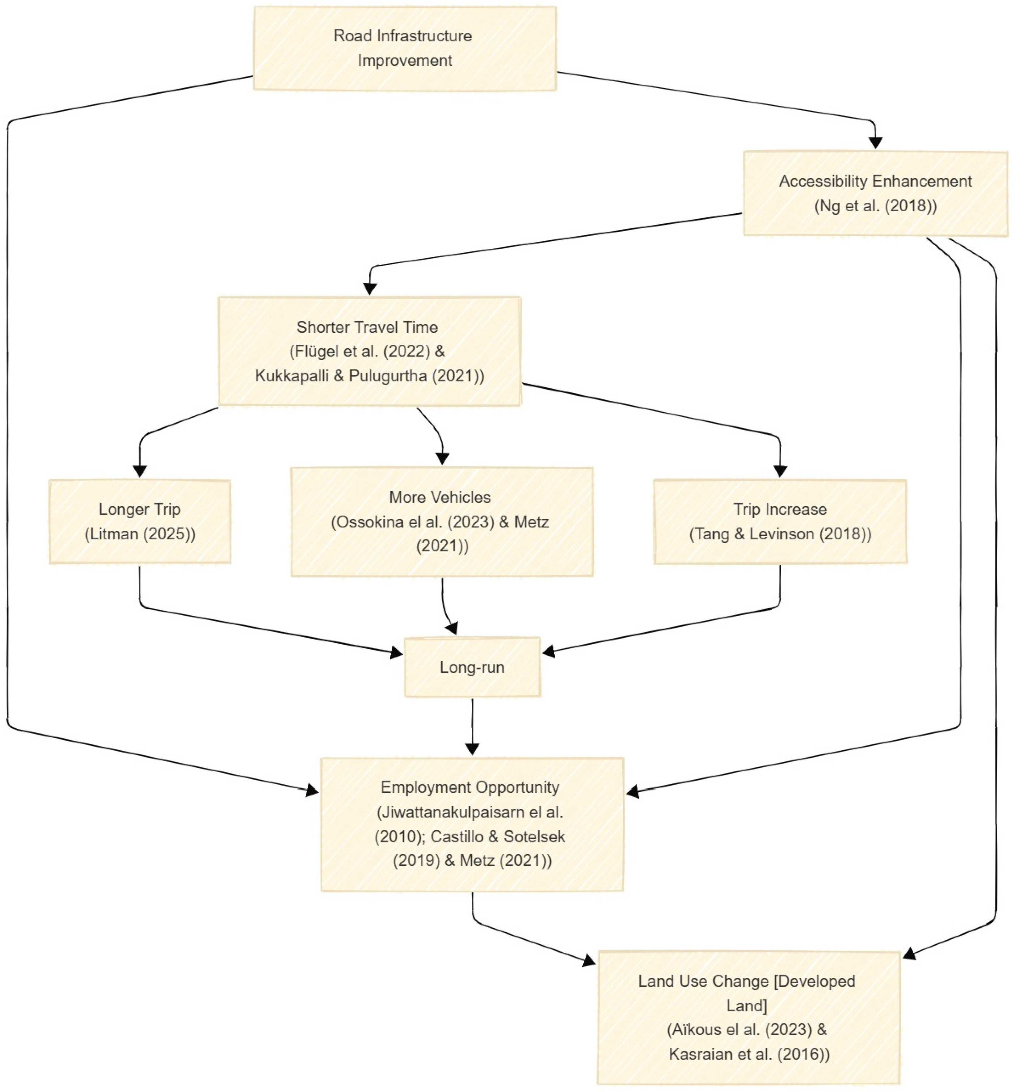
There is little doubt among transportation researchers that improving or expanding road capacity leads to increased vehicle use [14,15]. Road improvements follow the fundamental principles of economics: when the price of some goods decreases, an individual tends to consume more of those goods [10]. In other words, wider and new roads increase traffic speeds and reduce travel costs, thereby inducing additional vehicle travel [16,17,18]. In the short time frame, residential and employment locations remained fixed, and faster peak period road speeds pulled drivers from alternative routes, modes, and times of day to use those improved roads [19]. Then, in the long run, this additional traffic encourages additional social and economic activities to relocate around these improved transportation networks [14,20,21,22,23,24,25]. Vice versa, changes in land use influence travel patterns, determining traffic flows on roads, which has led to improving those road facilities [13,26].
Researchers use different modeling techniques to improve the understanding of road development and land use change. Nelson et al. [27] conducted a study in Colombia using multinomial, nested, and random parameter models to uncover the impact of road resurfacing and deforestation. The study could not find any direct connection between road improvements and deforestation due to particular trees found in remote areas with high elevations and steep slopes. Levinson et al. [4] developed A Simulator of Integrated Growth of Network Growth and Land Use (SIGNAL) model to investigate the co-evolution of transportation networks and land-use development. The study combined travel demand, road investment, accessibility, and land use models to develop this composite model. Rui and Ban [28] developed a dynamic growth model that combines two submodels: (1) a vector road growth model and (2) a grid land use model for long-term urban growth. Patarasuk and Binford [10] conducted a longitudinal study from 1986 to 2006 in Thailand, during which the land cover change and the construction of new roads were observed. The study employed a 7-km buffer along the road and observed land cover changes within the buffer area to establish a relationship between land use and road improvement. Alphan [29] examined the relationship between road development and changes in agricultural land use. The study divided the area into fishnets and calculated the percentage change in landscape and road density to determine the correlation. Mo et al. [30] conducted a study in China to assess the ecological risk associated with road expansion using ecological risk indices and road network kernel density. Zhao et al. [6] utilized land use and land cover data, as well as kernel density of road networks, to perform overlay and regression analysis, exploring the relationship between road improvements and land use.
Most studies used microsimulation or density-based methods to explore the relationship between road improvements and land use. However, there is a significant gap in the recent literature regarding the differentiation of land use patterns due to road improvements in rural and urban areas and whether land use changes occurred solely due to road improvements or also as a result of natural growth resulting from population increases. This study aims to fill this crucial gap. We test the hypothesis that some factors may differently impact land development. Specifically, we analyze the effect on land development by employment, improvements in road infrastructure, and mobility.
We study the relationship between infrastructure (road) development, employment, amount of travel, and land use change in the physical world. The definitions of what constitutes developedland density, employment density, road infrastructure improvement, urban and rural are provided below.
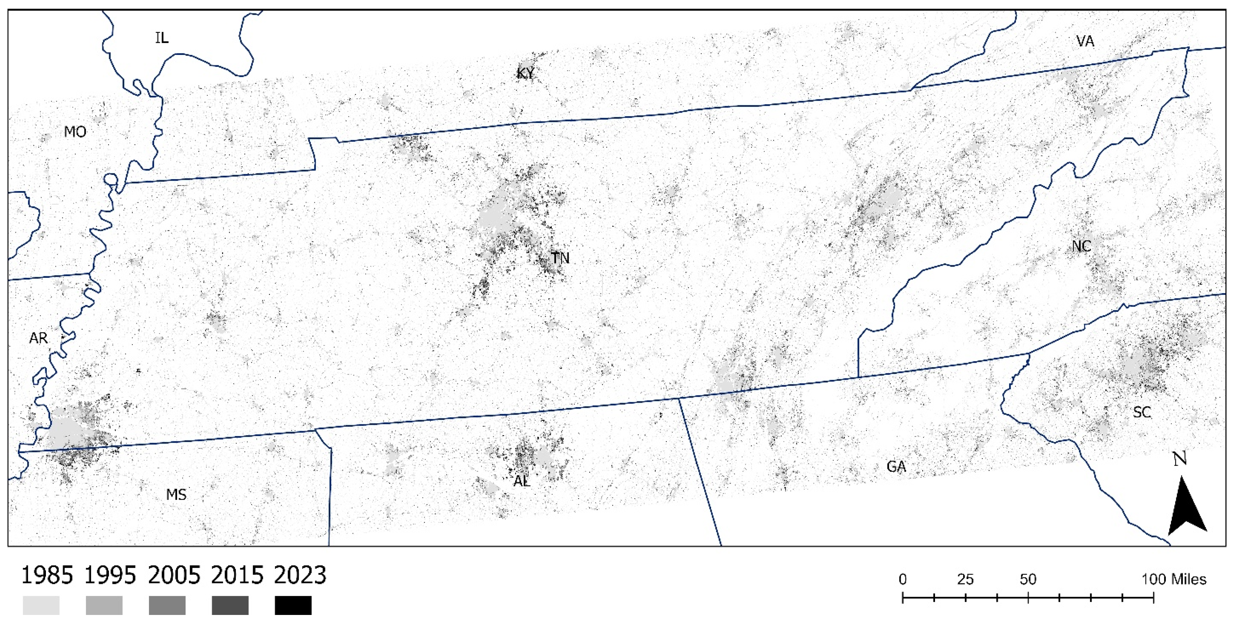
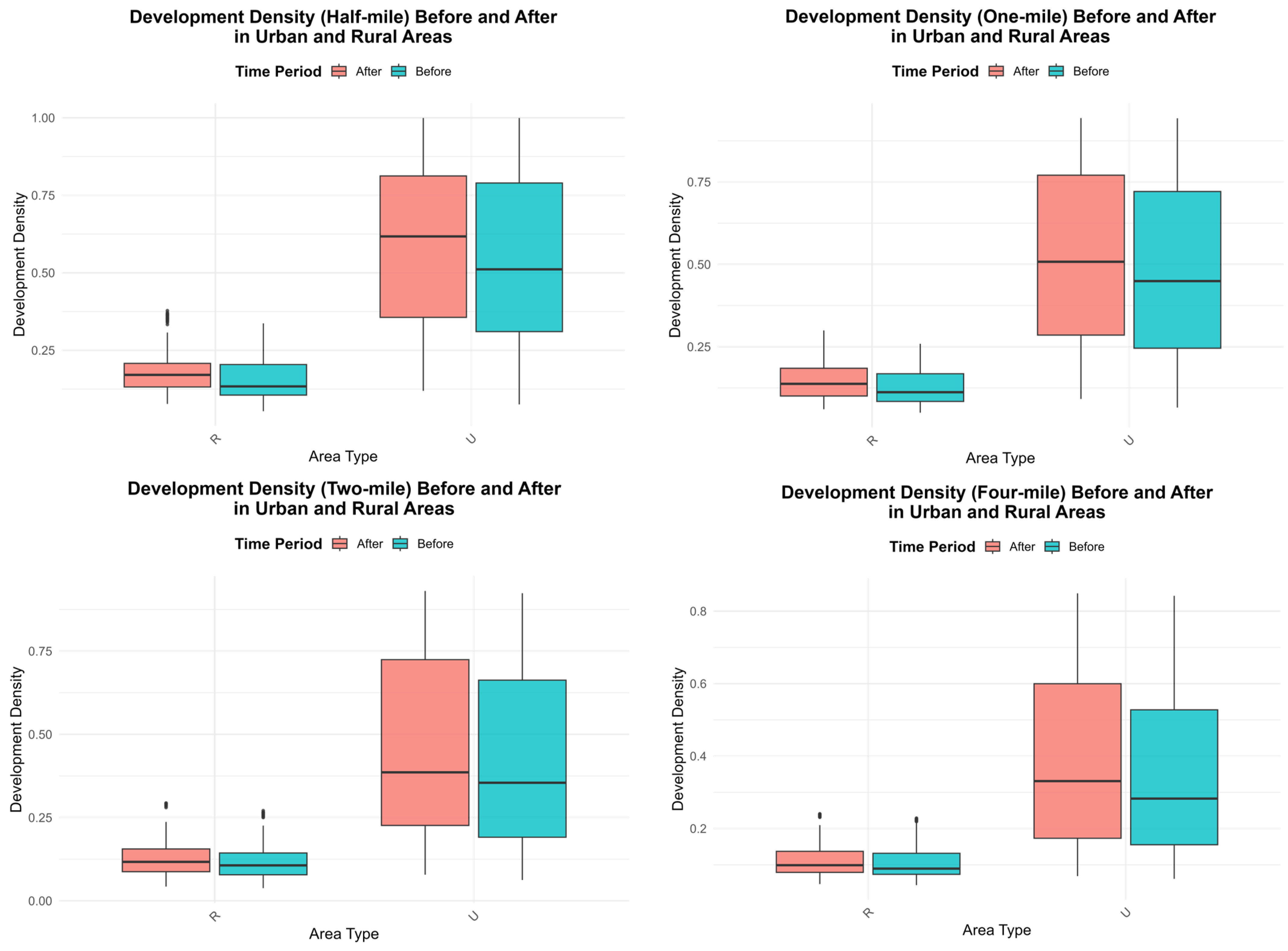
In this research, developed land represents altered landscape (vs. undeveloped land represented by natural land uses), which has specific uses such as roads and other types of infrastructure. This land cover represents four categories: developed open space, developed low Intensity, developed medium Intensity, and developed high Intensity (for the detailed definitions, please refer to the USGS Annual National Land Cover Dataset [NLCD]). Growth of developed land during 1985–2023 represents land use changes (also defined here as land development) during this period, and it is measured in this study by a developed land density (which was computed by dividing the total developed area by the buffer area around each road improvement site) described in detail in the subsection on Land Cover.
Road infrastructure improvement is defined as enhanced traffic vehicle capacity via line widening, construction of a new road, and other improvements in the road infrastructure. In this study, road improvement (interchangeably referred to as the road improvement projects and the study sites) occurred at the sites represented by the segments in the road network that have experienced such improvement. Eighty-four study sites (also referred to as road projects) in total were used in the study. Buffer areas were established around each road improvement site, including 0.5 miles, 1 mile, 2 miles, and 4 miles, to study the effect of the distance on changes in developed land.
Employment density measures economic activity, which influences land use patterns through land conversion into developed (i.e., built-up areas) by stimulating job creation and attracting investment. Employment density was calculated as the total number of jobs by summing all industrial categories divided by the respective buffer area around each road improvement site.
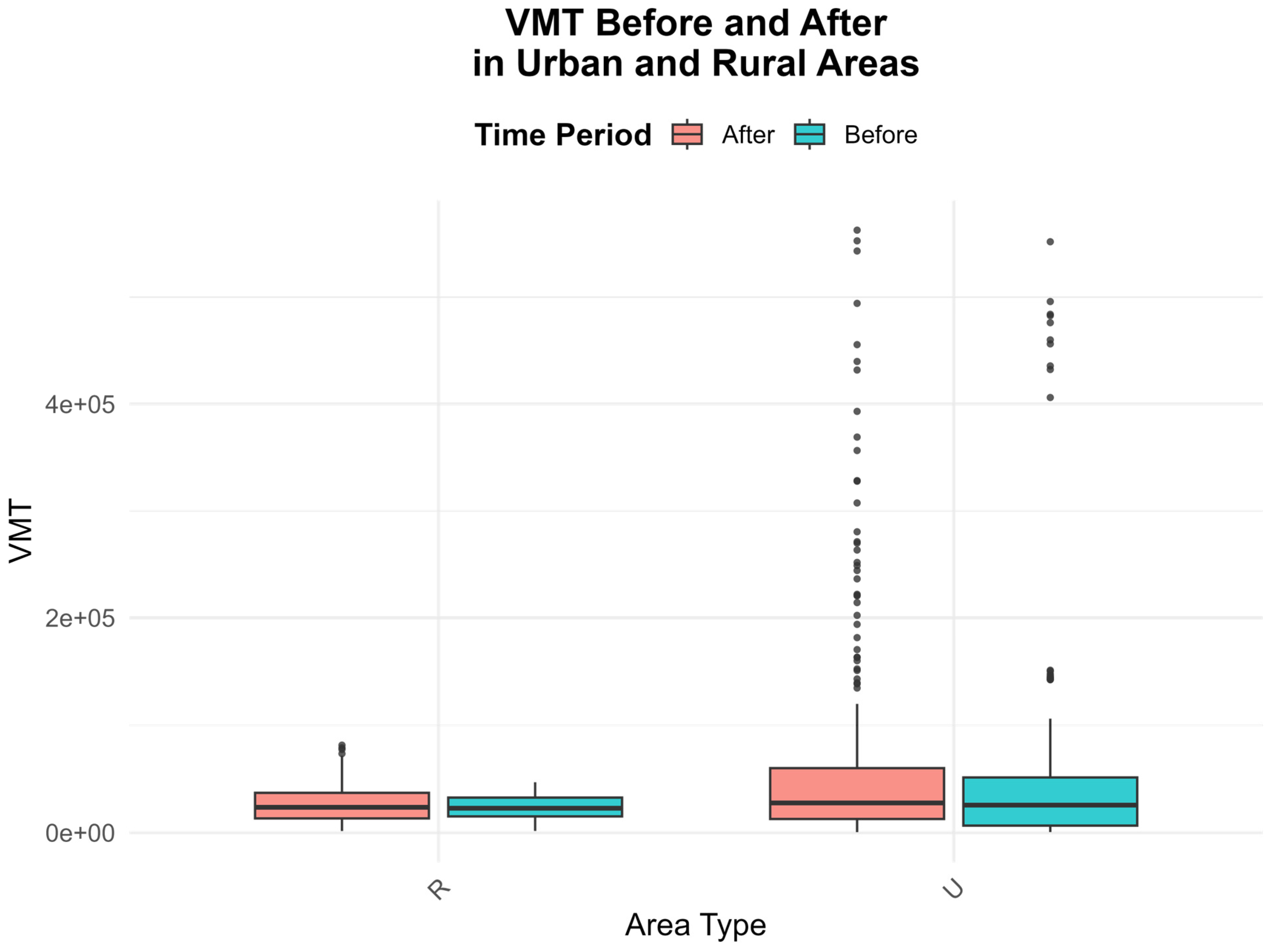
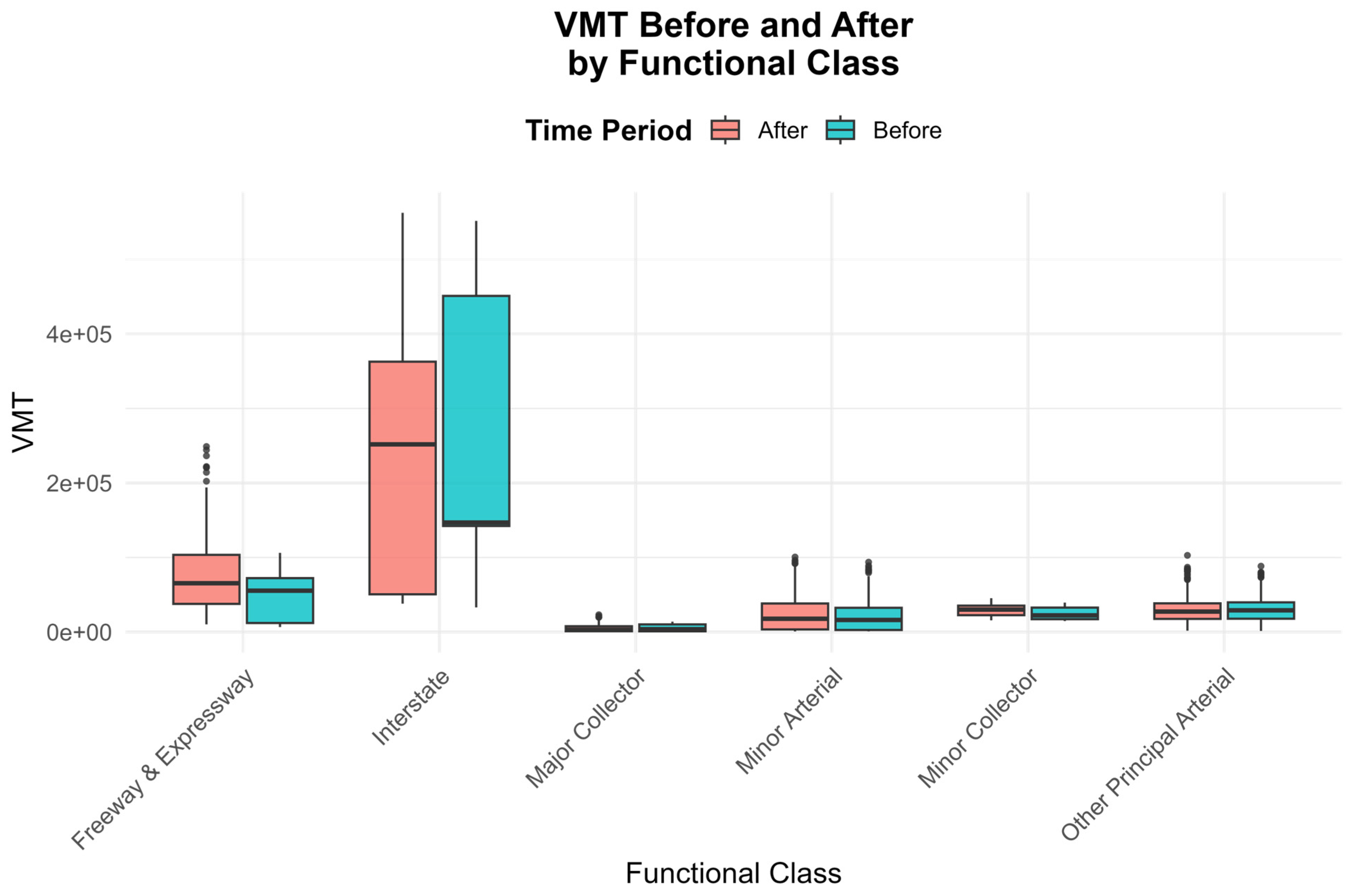
Mobility is proxied by the amount of travel. Increased mobility (i.e., travel demand) due to improvements in road infrastructure (e.g., by adding new roads) can ultimately induce changes in land use patterns. Here, mobility is measured by vehicle miles traveled (VMT) computed by using traffic data (i.e., Annual Average Daily Traffic (AADT) obtained from the Tennessee Traffic Information Management and Evaluation System (TN-TIMES) maintained by the Tennessee Department of Transportation (TDOT). Traffic data were linked with the study sites. A detailed description of the calculation is found in the subsection titled Traffic Data in Data and Data Imputation section.
Rural/urban classification has been used for the identification of the study site location. The rural/urban definitions come from the TN-TIMES classifying if the road is situated in a rural or urban area. A location within urbanized regions defines an area as urban and as rural otherwise.
We utilize real-time traffic data collected before and after the construction of road improvement or development projects and integrate it with employment data in developing a model to estimate the impact of developed land changes in rural and urban areas of Tennessee. The conceptual framework is presented in Figure 1. Additionally, this research aimed to connect the physical dimensions of transportation infrastructure with the developing metaverse technology, which could redefine this concept by offering experiences in virtual environments. Metaverse technology continuously involves and mixes with various aspects of our day-to-day lives, which makes it extremely important to explore its potential for integration into real-world transportation [31,32,33]. This research examines the case studies of Tennessee road improvement and its relation with developed land growth to provide a comprehensive understanding of the potential challenges and opportunities in emerging virtual real estate.

2. Materials and Methods

2.1. Study Area

Tennessee is located in the southeastern United States. Its diverse geography ranges from the Appalachian Mountains in the east to the rolling plains of Middle and West Tennessee. This diversity influences transportation networks, land development patterns, and urban growth dynamics. The state has well-developed transportation networks, including major interstate highways such as I-40, I-24, and I-75, which facilitate regional connectivity. This study comprises 84 road improvement projects throughout Tennessee (Figure 2).
It focuses on the relationship between road infrastructure improvements, VMT, employment density, and development density across urban and rural contexts. The earliest road improvement was completed in 2000, and the latest was completed in 2018. Of these 84 study sites, 35 are in rural areas, and 49 are in urban areas. Most improvement road projects fall within the “Other Principal Arterial” functional class, a classification system that groups roads by their function and importance in the transportation network (see Figure 3). The second highest functional class is the “Minor Arterial”. The number of other functional classes in the study area is under ten. This research analyzes changes in land development patterns at varying buffer distances (half-, one-, two-, and four-mile zones) to assess the spatial impact of transportation investments on regional growth.

2.2. Data and Data Imputation

2.2.1. Traffic Data

The shapefiles for the study sites have been obtained from the TDOT. The associated traffic data AADT were collected from the TN-TIMES which have been subsequently linked with these eighty-four study sites (also referred to as road projects). After collecting AADT data for respective road projects, VMT is calculated using Equation (1). It quantifies the total distance traveled by all vehicles within a specified geographic region over a defined time frame, typically one year [34].
V M T = A A D T × L e n g t h
Additionally, data were also collected from the TN-TIMES on the functional road classification and whether the road project is in a rural or urban area. Figure 3 illustrates a distribution of study sites by their functional class. This study utilized data from 10 years preceding and following project completion for analysis. For example, if a road project was completed in 2010, this study used data from 2000 to 2009 for the pre-project implementation period and from 2011 to 2020 for the post-project implementation period. This study excluded the year of completion from the analysis.
The boxplot shown in Figure 4 indicates that urban areas (labeled as U and rural areas are labeled as R) exhibit more significant variation and higher VMT levels compared to rural areas over the pre- and post-project implementation periods (also referred to as before and after period, respectively). While the differences in VMT before and after are not particularly substantial, there are noteworthy variations in the distribution (see Figure 4). Both urban and rural areas exhibit comparable median VMT values before and after, although urban areas display a broader distribution.
Figure 5 indicates that major roadways, particularly interstates, have undergone more significant changes in VMT due to road improvement. The data reveals the highest VMT values during the after period, characterized by a broader interquartile range and more significant variability compared to the before period, which can be attributed to enhancements in interstate roads. The median VMT for interstates appears to be higher in the after period, suggesting a potential increase in travel demand on these routes. In contrast, lower-tier transportation networks display a more stable distribution of VMT, indicating relatively minor fluctuations over time.

2.2.2. Employment Data

This study utilized the United States Census Bureau “OnTheMap” web service to collect employment data, which uses 2-digit NAICS codes to categorize industries into classes. The employment data from 2002 to 2022 was sourced from the website as point features, and the total number of jobs was calculated by summing all NAICS categories. Subsequently, the employment data was spatially joined and integrated with each buffer, allowing for the calculation of employment density in each buffer area by dividing the total employment by the buffer area. Figure 6 illustrates the employment density before and after the road improvement project across various rural and urban buffer areas in Tennessee. This figure provides a comparative overview of employment density across urban and rural regions. Urban areas (U) consistently display higher employment density throughout all buffer scenarios during the periods of before and after road improvement than rural areas (R), with a more pronounced interquartile range and median values. In contrast, rural areas show relatively low employment density, with minimal variation between the periods before and after the improvements.
Urban employment density shows some changes following improvements, yet the median values remain relatively stable, suggesting a localized increase rather than broad-based employment growth. The heightened dispersion observed in the post-improvement period may indicate the emergence of new job opportunities in specific areas attributable to enhanced accessibility and mobility. These findings point to a more significant impact of road network improvements on urban employment density than rural regions. The increased dispersion in urban employment density may reflect localized economic growth, likely driven by better access to job centers.

2.2.3. Land Cover

Due to the nature of the research studying the land use changes around infrastructures, we utilized satellite-based land use land cover data and used GIS to extract the percent of developed land. This study utilized the USGS Annual National Land Cover Dataset (NLCD) to calculate development density within the study area. The 1985–2023 NLCD data were accessed from the Multi-Resolution Land Characteristics (MRLC) consortium. The dataset classifies land cover into 20 categories, which were reclassified into broader categories for this analysis (see Table 1).
Following reclassification, land cover data were clipped to half-, one-, two-, and four-mile buffers around each study site. Development density was then calculated by determining the number of pixels classified as “Developed.” Since the NLCD dataset has a 30-m resolution, each pixel represents 900 square meters (30 m × 30 m). The total number of developed pixels was multiplied by 900 square meters and converted to square miles to estimate the developed area within each buffer zone. Finally, development density was computed by dividing the total developed area by the respective buffer area. Figure 7 shows the urban growth in Tennessee from 1985 to 2023.
In urban areas, a notable increase in development density is observed after construction, as evidenced by the shifts in the median and interquartile range depicted in the boxplots (see Figure 8). Conversely, development density in rural areas remains relatively stable, with only slight variations in both the median and whisker ranges. The buffer zones of half a mile and one mile exhibit the most significant differences in development density within urban settings. In contrast, development density patterns illustrate a broader spatial dispersion effect at larger buffer zones of two and four miles. However, urban areas continue to experience more substantial growth compared to their rural counterparts.

2.3. Methodology

This study estimated a predictive model using data from 84 study sites and considered four scenarios for buffer zones of (1) 0.5 miles, (2) 1 mile, (3) 2 miles, and (4) 4 miles. Figure 9 shows the detailed flowchart of the methodological application. Study sites represent the segments in the road network that have experienced improvement, such as line widening, thereby enhancing traffic vehicle capacity (see Figure 1, which shows the location of the study sites). The initial dataset comprised 1680 observations spanning data over 10 years. However, missing observations can be problematic for the model; researchers usually exclude those missing or incomplete observations from the dataset [27].
Accordingly, incomplete and missing entries have been excluded. The final sample size was 1245. In this analysis, development density served as the dependent variable. VMT, employment density, rural/urban classification used for the study site location, and a time indicator for the pre- and post-project implementation periods (coded as before/after, respectively) were used as explanatory variables. The rural and urban classifications and the time indicator were encoded as 0–1 dummy variables. Specifically, the urban area was coded as 1 and the rural area as 0, with the time indicator marked as 1 for the period after completion and 0 for the before-project implementation period. This study employed a logarithmic form of development density, employment density, and VMT in the predictive model.

Modeling Approach

This study utilizes an Ordinary Least Squares (OLS) regression model to analyze the relationship between development density, key transportation variables, and socioeconomic factors. Specifically, to avoid multicollinearity, we checked whether independent variables are correlated by calculating the Variance Inflation Factor (VIF) and used a common rule of thumb with the VIF values greater than 5 to indicate moderate multicollinearity. We additionally tested for heteroskedasticity in our linear regression model and examined if the error terms are normally distributed in a residual analysis. In the residual plot, a fairly constant variance of the residuals is observed across the range of fitted values. This approach aligns with contemporary practices in land use modeling, where OLS regression combined with diagnostic tests such as VIF and residual analysis are used to ensure model robustness and validity [35,36]. The dependent variable, development density, is log-transformed to address skewness and enable elasticity-based interpretations. The explanatory variables encompass log-transformed VMT, log-transformed employment density, rural/urban classification, and a temporal indicator that differentiates between pre- and post-road construction periods. The model is specified as follows:
log D e v D e n s i t y i = β 0 + β 1 log V M T i + β 2 log E m p D e n s i t y i + β 3 R u r a l U r b a n i + β 4 B e f o r e A f t e r i + ϵ i
where,
log D e v D e n s i t y i represents the log-transformed development density for observation i.
log E m p D e n s i t y i represents the log-transformed employment density for observation i.
log V M T i denotes the log-transformed vehicle miles traveled.
R u r a l U r b a n i is a binary indicator variable (1 = urban, 0 = rural).
B e f o r e A f t e r i is a binary variable distinguishing post-construction (after = 1) from pre-construction (before = 0) periods.
ϵ i is the error term, and
β 0 ; β 1 ; β 2 ; β 3 ; β 4 are regression coefficients to be estimated.
All continuous variables, including development density, VMT, and employment density, have been log-transformed to mitigate potential heteroskedasticity, improve normality, and facilitate coefficient interpretation as elasticities. The empirical analysis was conducted using Python 3.12.1 with the “statsmodels package” version 0.14.4 for regression estimation.

3. Results

Table 2 displays the descriptive statistics of the dependent and explanatory variables. The descriptive statistics indicate that as the distance from the road network increases, development and employment density decrease. An OLS model was performed for each buffer distance to analyze the relationship between the road network and development activities further. To check the model reliability, we test the multicollinearity and heteroskedasticity. Figure 10 shows the VIF scores of variables and a plot of residual vs. fitted values. VIF scores for all the variables in all models are below 5, indicating no multicollinearity concern. Regarding heteroskedasticity, the plot of the residual vs. fitted values for the half-mile buffer reveals mild heteroskedasticity. However, with increasing buffer distance, the variance becomes more homogeneous.

3.1. Half-Mile Buffer Model

The OLS regression produced an R-squared value of 0.798, suggesting that the chosen explanatory variables account for approximately 79.8% of the developed land use density variance. The adjusted R-squared value of 0.797 further substantiates the model’s robustness by considering the number of explanatory variables included. Additionally, the F-statistic of 1226 (p < 0.00) confirms the overall significance of the half-mile buffer model (see Table 3).
In the model, employment density is strongly correlated with developed land use. A unit increase in log employment density corresponds to an approximate 17.45% increase in developed land use (see Table 4), underscoring the significant role of employment hubs in driving urbanization. Figure 11 shows the coefficient plot and predicted vs observed plot. Coefficient plot showing the estimated effects of each explanatory variable in the regression model. Dots represent point estimates, and horizontal lines represent 95% confidence intervals. The red dashed vertical line at zero indicates the null effect. On the other hand, the scatterplot compares observed values with predicted values from the regression model. Each dot represents observation. The red dashed line is the 45-degree reference line, indicating perfect agreement between predicted and observed values. Points closely aligned with the line suggest a better model fit. Road improvement projects lead to an increase in VMT. In the half-mile model, the impact of VMT is relatively modest; specifically, a unit increase in log VMT is associated with a 0.71% rise in development density, indicating that mobility patterns contribute to changes in land use.
The positive coefficient for the “Before/After” indicator suggests that periods following road projects show higher development density compared to the conditions before the projects were implemented. This finding reinforces the hypothesis that improvements in road infrastructure stimulate land development within the affected buffer zone. Additionally, urban areas exhibit significantly higher development density than rural areas, with a 4.8% increase indicating that urbanized regions respond more markedly to infrastructural enhancements than rural zones.
The estimated OLS regression equation for developed land use within a half-mile buffer of the road project is as follows:
l o g ( D e v e l o p m e n t   D e n s i t y )                                             = 0.0421 + 0.0071 × l o g ( V M T )                                             + 0.1745 × l o g ( E m p l o y m e n t   D e n s i t y )                                             + 0.0217 × ( B e f o r e _ A f t e r ) + 0.0480 × ( R u r a l _ U r b a n )

3.2. One-Mile Buffer Model

The model exhibits significantly greater explanatory power than the half-mile buffer model, as evidenced by an R-squared value of 0.840. This indicates that the chosen predictors account for 84.0% of the variance in development density. The adjusted R-squared value of 0.840 implies a minimal risk of overfitting. Additionally, the model’s F-statistics of 1628 (p < 0.00) further underscores its statistical significance (see Table 5).
In the one-mile buffer model, employment density again emerges as the most significant determinant of developed land use. Figure 12 illustrates the coefficient plot and predicted vs observed plot for one-mile buffer model. A one-unit increase in log employment density corresponds to an approximate 20.82% rise in development density, which provides 3.37% more explanatory power than the half-mile buffer model. In this context, the explanatory power of VMT increases from 0.71% to 0.78%, indicating that heightened travel demand is linked to greater development density (see Table 6). Urban areas demonstrate a higher development density than rural areas, though the effect size is smaller than that observed in the half-mile buffer model. This suggests that the impact of urbanization diminishes as the buffer zone expands, likely reflecting patterns of suburbanization. The estimated OLS regression Equation (4) represents the model for developed land use within a 1-mile buffer of the road project.
l o g   ( D e v e l o p m e n t   D e n s i t y )                                             = 0.0955 + 0.0077 × l o g   ( V M T )                                             + 0.2082 × l o g   ( E m p l o y m e n t   D e n s i t y )                                             + 0.0182 × ( B e f o r e _ A f t e r ) + 0.0183 × ( R u r a l _ U r b a n )

3.3. Two-Mile Buffer Model

The two-mile buffer model demonstrates considerable explanatory power, boasting an R-squared value of 0.870. This indicates that the model accounts for 87.0% of the variance in development density. The adjusted R-squared value of 0.870 further substantiates the robustness of these findings. Additionally, the F-statistics of 2079 (p < 0.00) highlight the overall significance of the model (see Table 7).
Employment density remains the most significant predictor, with a one-unit increase resulting in a 22.16% increase in development density (see Table 8). This effect size is slightly greater than that observed in smaller buffer models, indicating that employment-driven urbanization is more pronounced at larger spatial scales. In contrast to smaller buffer models, the influence of VMT shows a slight increase, suggesting that enhanced mobility accessibility plays a more crucial role in development at larger scales. Furthermore, unlike in the smaller buffer models, rural-urban classification is no longer statistically significant (p > 0.05). Figure 13 displays the coefficient plot and predicted vs observed plot, where red line for coefficient indicates the null effect and in predicted vs observed plot 45 degree red line representing the model fit line.

3.4. Four-Mile Buffer Model

The four-mile buffer model exhibits the highest explanatory power among all buffer sizes, with an R-squared value of 0.920, indicating that the selected variables explain 92.0% of the variance in development density. The adjusted R-squared (0.920) confirms the robustness of these findings (see Table 9). The model is highly significant overall (F-statistics = 3576, p < 0.00), reinforcing the reliability of the estimated relationships.
In all four models, employment density remains the primary predictor of land development. In the four-mile buffer model, a one-unit increase in log-employment density results in a 21.63% increase in development density, underscoring the vital role of economic activity in urban expansion (see Table 10). Figure 14 illustrates the coefficient plot and predicted vs observed plot for visualizing the regression results. Each black dot in the predicted vs observed plot represents each observation and red line represents the model fit line. This effect size remains consistent across various buffer distances, indicating that employment-driven urbanization extends beyond immediate proximity to roadways and influences a larger area. While the effect of VMT remains positive and statistically significant, its influence decreases when examined at broader spatial scales. Specifically, a unit increase in log-VMT corresponds to a 0.63% increase in development density, suggesting that regional mobility has an impact, but this effect is weaker at larger distances. Additionally, unlike the findings from smaller buffer models, the coefficient for rural-urban classification is negative, indicating that rural areas within a 4-mile buffer have experienced relatively lower development density than their urban counterparts. This observation suggests that the urbanization effect diminishes with increasing distance from the road project, resulting in a lesser developmental response in rural areas.
l o g ( D e v e l o p m e n t   D e n s i t y )                                             = 0.084 + 0.0063 × l o g ( V M T )                                             + 0.2163 × l o g ( E m p l o y m e n t   D e n s i t y )                                             + 0.0109 × ( B e f o r e _ A f t e r ) 0.0197 × ( R u r a l _ U r b a n )

4. Discussion

Both physical and digital land can be used for various purposes, including land development. Understanding how land is developed in the real world helps one understand how digital land and virtual real estate can grow. One way how physical land can be used and developed is by building various structures and providing and improving infrastructure, both activities are shaped by land use planning and zoning. Within the metaverse, digital land can be “developed” by constructing digital structures and creating virtual economies.
Various factors, including employment, location, utility, engagement potential (e.g., high-traffic areas), and other factors, may shape digital land’s attributes (e.g., its growth, value, etc.). The potential growth of digital land is limitless. Factors like infrastructure or neighborhood amenities affect the characteristics of the physical land and real estate (value, growth). The growing convergence between physical infrastructure and digital twins or metaverse environments offers new avenues for urban planning. Hudson-Smith [37] argues that immersive digital mirrors of cities could reshape urban planning, while Dembski et al. [38] and Hassan et al. [39] highlight the role of digital twins in managing real-world infrastructure through virtual environments.
Gaps exist in prior studies regarding whether changes in land use patterns occur due to road improvements in rural and urban areas and whether these changes are a result of road improvements or natural growth resulting from population increases. We fill this crucial gap by using real-time traffic data in the periods before and after road infrastructure improvement. We develop a model to estimate the extent to which various development factors, including employment, road infrastructure, and locality (rural and urban areas), contribute to land use changes in Tennessee.
Detailed geospatial mapping enables urban designers to create sophisticated virtual replicas of roads, buildings, parks, green spaces, landmarks, and other elements of city infrastructure and topography. Using virtual reality, real-world roads can be made safer, and vice versa.
By bridging both physical and virtual spaces, next-generation services can be provided to residents, including digital shopping complexes, virtual counterparts of city parks and landmarks, and other cultural experiences. Physical developments require foundational infrastructure, such as transportation networks, electrical grids, and telecommunications systems, while virtual developments necessitate digital infrastructure, including hardware, software, network connectivity, and data centers, to function effectively. Virtual developments, like the metaverse, rely on real-time, high-quality, fast, and reliable network connectivity. Here, we examine the relationship between infrastructure development (in this case, roads) and land use change in the physical world, which may help us understand this connection.

5. Conclusions

There are vast prospects for the metaverse and virtual real estate. However, the prospective impacts of transportation development in the metaverse have been questioned in this paper. In this paper, we present a case study aimed at enhancing our understanding of the factors influencing land development, including employment, travel volume, road improvements, and urban growth. Developed land (the “development”) was estimated within each buffer zone around the improved road infrastructure (referred to as road projects) and measured in square miles, and subsequently, development density was computed by dividing the total developed area by the respective buffer area over 1985 to 2023. Change in development density enables us to estimate developed land growth (that is, urban growth) for the period of 1985 to 2023.
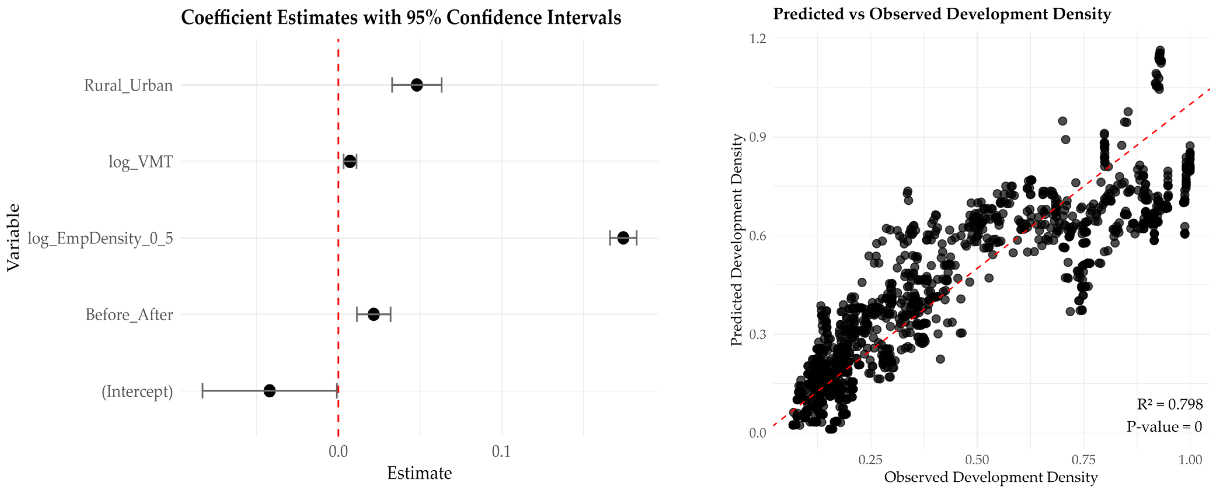
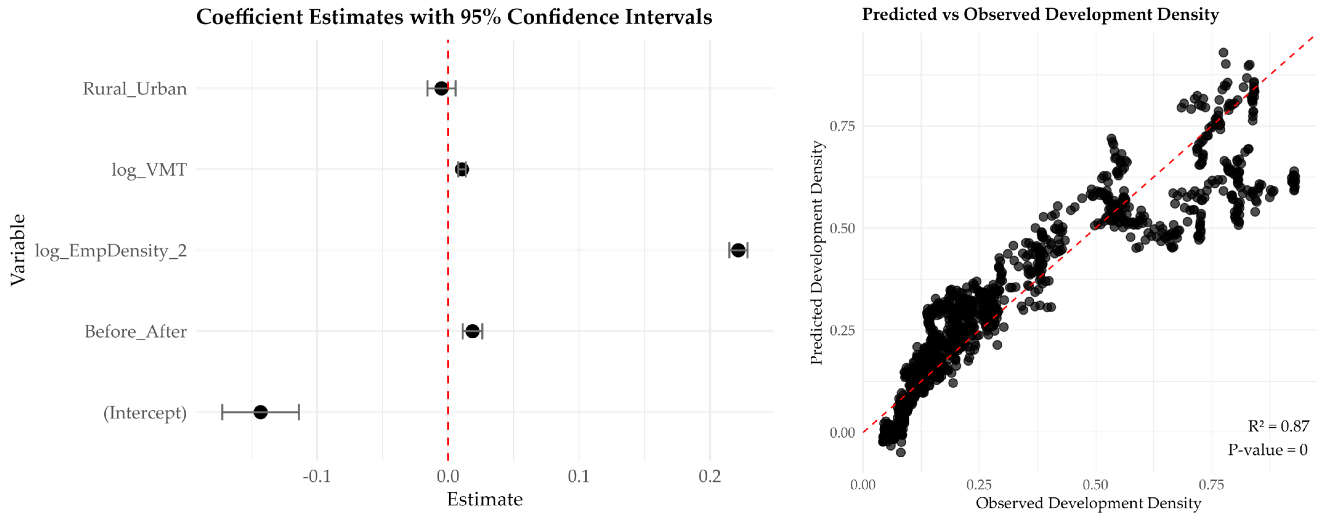
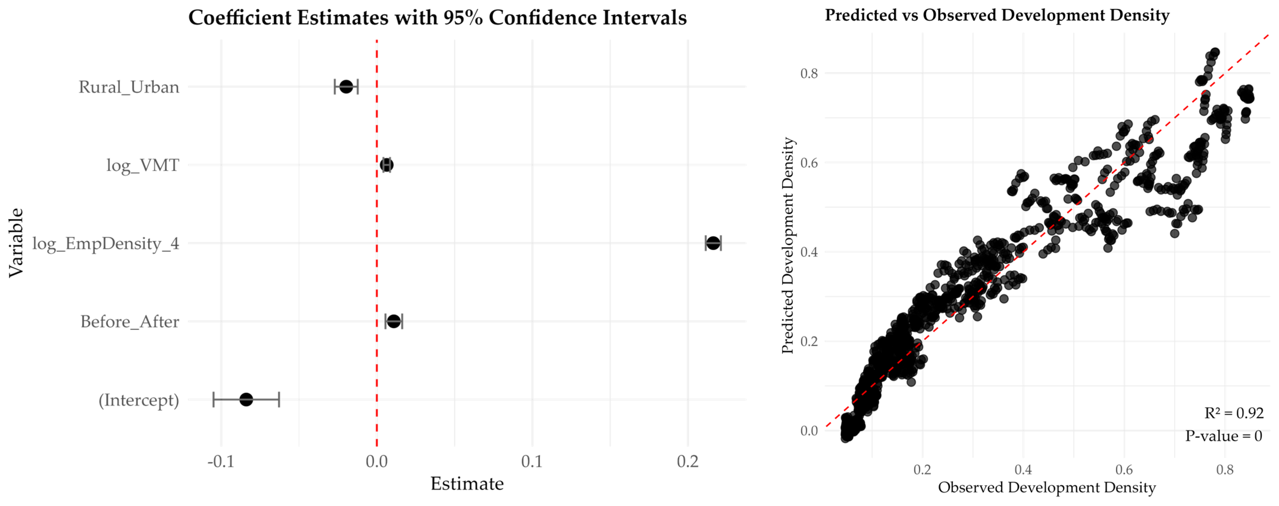
We find employment the primary predictor of developed land growth. The land development effect of employment stretches well beyond immediate proximity to road infrastructure providing a consistent strong impact over a larger area. Vehicle traffic (measured by VMT) provides a positive and statistically significant effect on land development (measured by development density); however, the land development effect of road infrastructure improvement decreases at broader spatial scales. In our study, it diminishes with increasing distance from the road, resulting in less development in rural areas.
This study has limitations. Data used in this analysis have been taken from the physical world potentially limiting our understanding of the impact of virtual environments on real-world experiences. Future research directions should focus on this impact to improve the quality of life for city residents and examine how metaverse-based principles can be used towards solutions to the problems inherent to urban infrastructure and governance systems of the physical world. One example of the application would be redefining urban landscapes to meet the needs of the emerging digital economy and infrastructure in the near future [40,41].
This research is crucial for informing future transportation planning, land-use policies, and sustainable growth strategies. The findings will help policymakers and planners understand how infrastructure changes affect urban expansion, employment accessibility, and regional development, providing valuable insights for future planning and policy development. Specifically, this research raises awareness about the prospects of virtual real estate. Recognizing these prospects of transportation improvement on land development suggests more integration of real-world data integration with the metaverse. Finally, this research bridges the impact of transportation systems, such as changes in travel behavior, employment, and urbanization patterns, with metaverse.

Author Contributions

Conceptualization, J.B. and A.A.; methodology, J.B. and A.A.; software, J.B.; formal analysis, J.B.; writing—original draft preparation, J.B. and A.A.; writing—review and editing, J.B. and A.A.; visualization, J.B.; supervision, A.A. All authors have read and agreed to the published version of the manuscript.

Funding

This research received no external funding.

Data Availability Statement

Traffic data can be accessed from TN-TIMES; Land cover data from MRLC sites; Employment Data from OnTheMap.

Acknowledgments

We acknowledge the support from TDOT, which provided us with the road improvement sites’ shapefiles and bulk data download access from TN-TIMES.

Conflicts of Interest

The authors declare that they have no conflicts of interest.

Abbreviations

The following abbreviations are used in this manuscript:
AADTAnnual Average Daily Traffic
OLSOrdinary Least Square
MaxMaximum
MinMinimum
NLDCNational Land Cover Dataset
RRural
Std DevStandard Deviation
TDOTTennessee Department of Transportation
TN-TIMESTennessee Traffic Information Management and Evaluation System (TN-TIMES)
UUrban
VMTVehicle Mile Traveled

References

  1. Angel, S.; Parent, J.; Civco, D.L.; Blei, A.; Potere, D. The Dimensions of Global Urban Expansion: Estimates and Projections for All Countries, 2000–2050. Prog. Plan. 2011, 75, 53–107. [Google Scholar] [CrossRef]
  2. Zhang, Q.; Wang, J.; Peng, X.; Gong, P.; Shi, P. Urban Built-up Land Change Detection with Road Density and Spectral Information from Multi-Temporal Landsat TM Data. Int. J. Remote Sens. 2002, 23, 3057–3078. [Google Scholar] [CrossRef]
  3. Liu, S.; Rong, J.; Zhou, C.; Gao, Y.; Xing, L. Temporal Heterogeneity in Land Use Effects on Urban Rail Transit Ridership—Case of Beijing, China. Land 2025, 14, 665. [Google Scholar] [CrossRef]
  4. Levinson, D.M.; Xie, F.; Zhu, S. The Co-Evolution of Land Use and Road Networks. 2007. Available online: https://papers.ssrn.com/sol3/papers.cfm?abstract_id=1748607 (accessed on 2 May 2025).
  5. Ng, C.P.; Law, T.H.; Jakarni, F.M.; Kulanthayan, S. Relative Improvements in Road Mobility as Compared to Improvements in Road Accessibility and Urban Growth: A Panel Data Analysis. Transp. Res. Part Policy Pract. 2018, 117, 292–301. [Google Scholar] [CrossRef]
  6. Zhao, G.; Zheng, X.; Yuan, Z.; Zhang, L. Spatial and Temporal Characteristics of Road Networks and Urban Expansion. Land 2017, 6, 30. [Google Scholar] [CrossRef]
  7. Weingroff, R.F. Federal Aid Highway Act of 1956: Creating the Interstate System. Fed. Aid Highw. Act 1956 Creat. Interstate Syst. 1996, 60, 10–17. [Google Scholar]
  8. Cervero, R. Road Expansion, Urban Growth, and Induced Travel: A Path Analysis. J. Am. Plann. Assoc. 2003, 69, 145–163. [Google Scholar] [CrossRef]
  9. Krugman, P. The Role of Geography in Development. Int. Reg. Sci. Rev. 1999, 22, 142–161. [Google Scholar] [CrossRef]
  10. Patarasuk, R.; Binford, M.W. Longitudinal Analysis of the Road Network Development and Land-Cover Change in Lop Buri Province, Thailand, 1989–2006. Appl. Geogr. 2012, 32, 228–239. [Google Scholar] [CrossRef]
  11. Stanilov, K. Accessibility and Land Use: The Case of Suburban Seattle, 1960-1990. Reg. Stud. 2003, 37, 783–794. [Google Scholar] [CrossRef]
  12. Diaconu, D.C.; Peptenatu, D.; Gruia, A.K.; Grecu, A.; Gruia, A.R.; Gruia, M.F.; Drăghici, C.C.; Băloi, A.M.; Alexandrescu, M.B.; Sibinescu, R.B. The Impact of Urban Expansion on Land Use in Emerging Territorial Systems: Case Study Bucharest-Ilfov, Romania. Agriculture 2025, 15, 406. [Google Scholar] [CrossRef]
  13. Aïkous, M.; Dubé, J.; Brunelle, C.; Champagne, M.-P. Highway Expansion and Impacts on Land Use Changes: An Event Study Approach. Transp. Res. Part Transp. Environ. 2023, 119, 103730. [Google Scholar] [CrossRef]
  14. Hymel, K. If You Build It, They Will Drive: Measuring Induced Demand for Vehicle Travel in Urban Areas. Transp. Policy 2019, 76, 57–66. [Google Scholar] [CrossRef]
  15. Tang, W.; Levinson, D.M. Deviation between Actual and Shortest Travel Time Paths for Commuters. J. Transp. Eng. Part Syst. 2018, 144, 04018042. [Google Scholar] [CrossRef]
  16. Flügel, S.; Halse, A.H.; Hartveit, K.J.L.; Ukkonen, A. Value of Travel Time by Road Type. Eur. Transp. Res. Rev. 2022, 14, 35. [Google Scholar] [CrossRef]
  17. Ossokina, I.V.; Van Ommeren, J.; Van Mourik, H. Do Highway Widenings Reduce Congestion? J. Econ. Geogr. 2023, 23, 871–900. [Google Scholar] [CrossRef]
  18. Kukkapalli, V.M.; Pulugurtha, S.S. Comparing Travel Time Performance-Based Measures to Assess the Effect of a Freeway Road Construction Project on Freeway and Connecting Arterial Street Links. Urban Plan. Transp. Res. 2021, 9, 319–335. [Google Scholar] [CrossRef]
  19. Litman, T.A. Generated Traffic and Induced Travel: Implications for Transport Planning; Victoria Transport Policy Institute: Victoria, BC, Canada, 2025. [Google Scholar]
  20. Bucsky, P.; Juhász, M. Long-Term Evidence on Induced Traffic: A Case Study on the Relationship between Road Traffic and Capacity of Budapest Bridges. Transp. Res. Part Policy Pract. 2022, 157, 244–257. [Google Scholar] [CrossRef]
  21. Volker, J.M.B.; Lee, A.E.; Handy, S. Induced Vehicle Travel in the Environmental Review Process. Transp. Res. Rec. 2020, 2674, 468–479. [Google Scholar] [CrossRef]
  22. Kantianis, D.; Polyzos, S.; Krabokoukis, T. Land Use Changes, Environmental Impact and Socio-Economic Effects of Road Infrastructure Mega Projects: The Combined Case of the Rio–Antirio Bridge and the Ionian Road in Greece. Land 2025, 14, 486. [Google Scholar] [CrossRef]
  23. Jiwattanakulpaisarn, P.; Noland, R.B.; Graham, D.J. Causal Linkages between Highways and Sector-Level Employment. Transp. Res. Part Policy Pract. 2010, 44, 265–280. [Google Scholar] [CrossRef]
  24. Metz, D. Economic Benefits of Road Widening: Discrepancy between Outturn and Forecast. Transp. Res. Part Policy Pract. 2021, 147, 312–319. [Google Scholar] [CrossRef]
  25. Laborda, L.; Sotelsek, D. Effects of Road Infrastructure on Employment, Productivity and Growth: An Empirical Analysis at Country Level. J. Infrastruct. Dev. 2019, 11, 81–120. [Google Scholar] [CrossRef]
  26. Kasraian, D.; Maat, K.; Stead, D.; van Wee, B. Long-Term Impacts of Transport Infrastructure Networks on Land-Use Change: An International Review of Empirical Studies. Transp. Rev. 2016, 36, 772–792. [Google Scholar] [CrossRef]
  27. Nelson, G.; De Pinto, A.; Harris, V.; Stone, S. Land Use and Road Improvements: A Spatial Perspective. Int. Reg. Sci. Rev. 2004, 27, 297–325. [Google Scholar] [CrossRef]
  28. Rui, Y.; Ban, Y. Urban Growth Modeling with Road Network Expansion and Land Use Development. In Proceedings of the Advances in Cartography and GIScience; Ruas, A., Ed.; Springer: Berlin/Heidelberg, Germany, 2011; Volume 2, pp. 399–412. [Google Scholar]
  29. Alphan, H. Analysis of Road Development and Associated Agricultural Land Use Change. Environ. Monit. Assess. 2017, 190, 5. [Google Scholar] [CrossRef] [PubMed]
  30. Mo, W.; Wang, Y.; Zhang, Y.; Zhuang, D. Impacts of Road Network Expansion on Landscape Ecological Risk in a Megacity, China: A Case Study of Beijing. Sci. Total Environ. 2017, 574, 1000–1011. [Google Scholar] [CrossRef]
  31. Han, Y.; Niyato, D.; Leung, C.; Miao, C.; Kim, D.I. A Dynamic Resource Allocation Framework for Synchronizing Metaverse with IoT Service and Data. In Proceedings of the ICC 2022-IEEE International Conference on Communications, Seoul, Republic of Korea, 16–20 May 2022; pp. 1196–1201. [Google Scholar]
  32. Deveci, M.; Gokasar, I.; Castillo, O.; Daim, T. Evaluation of Metaverse Integration of Freight Fluidity Measurement Alternatives Using Fuzzy Dombi EDAS Model. Comput. Ind. Eng. 2022, 174, 108773. [Google Scholar] [CrossRef]
  33. Mogaji, E. Metaverse Influence on Transportation: A Mission Impossible? Transp. Res. Interdiscip. Perspect. 2023, 22, 100954. [Google Scholar] [CrossRef]
  34. FHWA, none Federal Highway Administration (FHWA). Available online: https://www.fhwa.dot.gov/policy/23cpr/chap3.cfm (accessed on 2 May 2025).
  35. Kou, X.; Zhao, J.; Sang, W. Impact of Typical Land Use Expansion Induced by Ecological Restoration and Protection Projects on Landscape Patterns. Land 2024, 13, 1513. [Google Scholar] [CrossRef]
  36. Pourmohammadi, P.; Strager, M.P.; Dougherty, M.J.; Adjeroh, D.A. Analysis of Land Development Drivers Using Geographically Weighted Ridge Regression. Remote Sens. 2021, 13, 1307. [Google Scholar] [CrossRef]
  37. Hudson-Smith, A. Incoming Metaverses: Digital Mirrors for Urban Planning. Urban Plan. 2022, 7, 343–354. [Google Scholar] [CrossRef]
  38. Dembski, F.; Wössner, U.; Letzgus, M.; Ruddat, M.; Yamu, C. Urban Digital Twins for Smart Cities and Citizens: The Case Study of Herrenberg, Germany. Sustainability 2020, 12, 2307. [Google Scholar] [CrossRef]
  39. Umair Hassan, M.; Abdel-Afou Alaliyat, S.; Hameed, I.A. Toward the Creation of a Digital Twin Authoring Tool: A Smart Mobility Perspective in Smart Cities. IEEE Access 2024, 12, 111280–111292. [Google Scholar] [CrossRef]
  40. Tinmaz, H. Technology Giant South Korea’s Metaverse Experiences. In Metaverse: Technologies, Opportunities and Threats; Esen, F.S., Tinmaz, H., Singh, M., Eds.; Springer Nature: Singapore, 2023; pp. 305–322. ISBN 978-981-99-4641-9. [Google Scholar]
  41. Ruban, A. The Role of the Government in Metaverse Development in China and South Korea: A Comparative Analysis. Master’s Thesis, HSE University, Moscow, Russia, 2024. [Google Scholar]
Figure 1. Conceptual framework [5,13,16,17,18,19,23,24,25,26].
Land 14 01025 g001
Figure 2. Location map of study sites.
Land 14 01025 g002
Figure 3. Distribution of study sites based on “Functional Class”.
Land 14 01025 g003
Figure 4. VMT before and after road improvement in rural and urban areas in Tennessee.
Land 14 01025 g004
Figure 5. VMT before and after by functional classification.
Land 14 01025 g005
Figure 6. Employment Density Before and After Road Improvement Implementation in Rural and Urban Tennessee (top left—half a mile, top right—one mile, bottom left—two mile, and bottom right—four-mile buffer).
Land 14 01025 g006
Figure 7. Urban growth in Tennessee from 1985 to 2023.
Land 14 01025 g007
Figure 8. Development Density Before and After in Rural and Urban Tennessee (top left half-mile, top right one-mile, bottom left two-mile, and bottom right four-mile buffer).
Land 14 01025 g008
Figure 9. Flowchart of methodological application.
Land 14 01025 g009
Figure 10. Multicollinearity Diagnostics and Residual Analysis for Log-Transformed OLS Models.
Land 14 01025 g010
Figure 11. Coefficient estimation and predicted vs. observed graph (half-mile model).
Land 14 01025 g011
Figure 12. Coefficient estimation and predicted vs. observed graph (one-mile model).
Land 14 01025 g012
Figure 13. Coefficient estimation and predicted vs. observed graph (two-mile model).
Land 14 01025 g013
Figure 14. Coefficient estimation and predicted vs. observed graph (four-mile model).
Land 14 01025 g014
Table 1. Reclassified NLDC Data.
CodeNLCD Land ClassificationReclassified Land Cover
11Open WaterWater
12Perennial Ice Snow
21Developed (Open Space)Developed
22Developed (Low Intensity)
23Developed (Medium Intensity)
24Developed (High Intensity)
31Barren LandBarren Land
41Deciduous ForestForest
42Evergreen Forest
43Mixed Forest
51Dwarf ScrubShrubland
52Shrub
71Grassland/HerbaceousHerbaceous
72Sedge/Herbaceous
73Lichens
74Moss
81Pasture/HayCrops
82Cultivated Crops
90Woody WetlandsWetlands
95Herbaceous Wetlands
Table 2. Descriptive statistics.
VariablesMeanMaxMinStd Dev
Development Density (Half a mile)0.401.000.050.29
Development Density (One mile)0.350.940.050.27
Development Density (Two-mile)0.300.930.040.25
Development Density (Four-mile)0.260.850.040.22
VMT39,310.99562,657.32486.6062,704.90
Employment Density (Half a mile)5.5051.600.007.07
Employment Density (One mile)4.3725.930.004.77
Employment Density (Two-mile)3.7019.670.003.89
Employment Density (Four-mile)3.1317.400.003.49
Table 3. Half-mile buffer model statistics.
StatisticsValuesStatisticsValues
R-squared0.798Log-Likelihood1245.8
Adjusted R-squared0.797AIC−2482
F-statistics1226BIC−2456
Prob (F-statistics)0.00No. Observation1245
Table 4. Half-mile buffer model output.
VariableCoefficientStd. Errort-Statisticp-Value
Intercept−0.04210.021−2.0050.045
Log (VMT)0.00710.0023.5370.00
Log (EmpDensity)0.17450.00441.9730.00
Before/After0.02170.0054.1130.00
Rural/Urban0.0480.0086.2110.00
Table 5. One-mile buffer model statistics.
StatisticsValuesStatisticsValues
R-squared0.840Log-Likelihood1425.4
Adjusted R-squared0.840AIC−2841
F-statistics1628BIC−2815
Prob (F-statistics)0.00No. Observation1245
Table 6. One-mile buffer model output.
VariableCoefficientStd. Errort-Statisticp-Value
Intercept−0.09550.018−5.320.00
Log (VMT)0.00770.0024.3950.00
Log (EmpDensity)0.20820.00451.940.00
Before/After0.01820.0053.9930.00
Rural/Urban0.01830.0072.7390.006
Table 7. Two-mile buffer model statistics.
StatisticsValuesStatisticsValues
R-squared0.870Log-Likelihood1645.4
Adjusted R-squared0.870AIC−3281
F-statistics2079BIC−3255
Prob (F-statistics)0.00No. Observation1245
Table 8. Two-mile buffer model output.
VariableCoefficientStd. Errort-Statisticp-Value
Intercept−0.14320.015−9.6020.00
Log (VMT)0.01060.0017.2380.00
Log (EmpDensity)0.22160.00462.9810.00
Before/After0.01860.0044.8820.00
Rural/Urban−0.00510.005−0.9280.353
Table 9. Four-mile buffer model statistics.
StatisticsValuesStatisticsValues
R-squared0.920Log-Likelihood2056
Adjusted R-squared0.920AIC−4102
F-statistics3576BIC−4076
Prob (F-statistics)0.00No. Observation1245
Table 10. Four-mile buffer model output.
VariableCoefficientStd. Errort-Statisticp-Value
Intercept−0.0840.011−7.8170.00
Log (VMT)0.00630.0015.8770.00
Log (EmpDensity)0.21630.00287.0480.00
Before/After0.01090.0033.9810.00
Rural/Urban−0.01970.004−5.2290.00
Disclaimer/Publisher’s Note: The statements, opinions and data contained in all publications are solely those of the individual author(s) and contributor(s) and not of MDPI and/or the editor(s). MDPI and/or the editor(s) disclaim responsibility for any injury to people or property resulting from any ideas, methods, instructions or products referred to in the content.

