
Identification of Production–Living–Ecological Spatial Conflicts and Multi-Scenario Simulations in Extreme Arid Areas

Abstract
1. Introduction
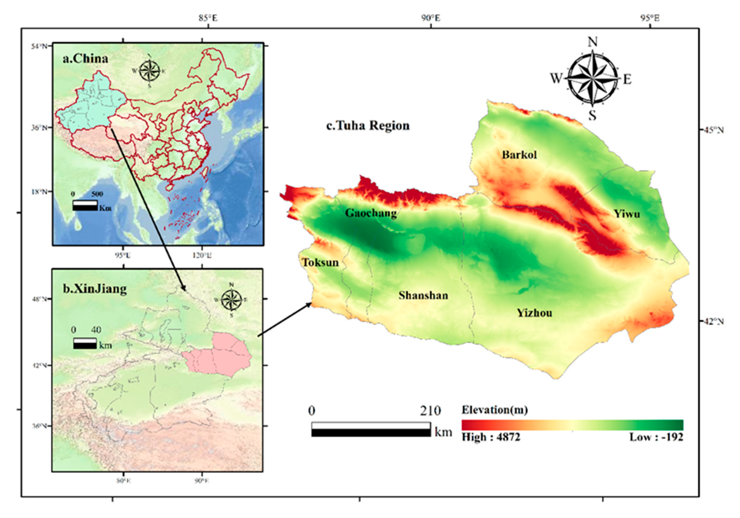
2. Study Area Overview and Data Sources
2.1. Study Area
2.2. Data Sources
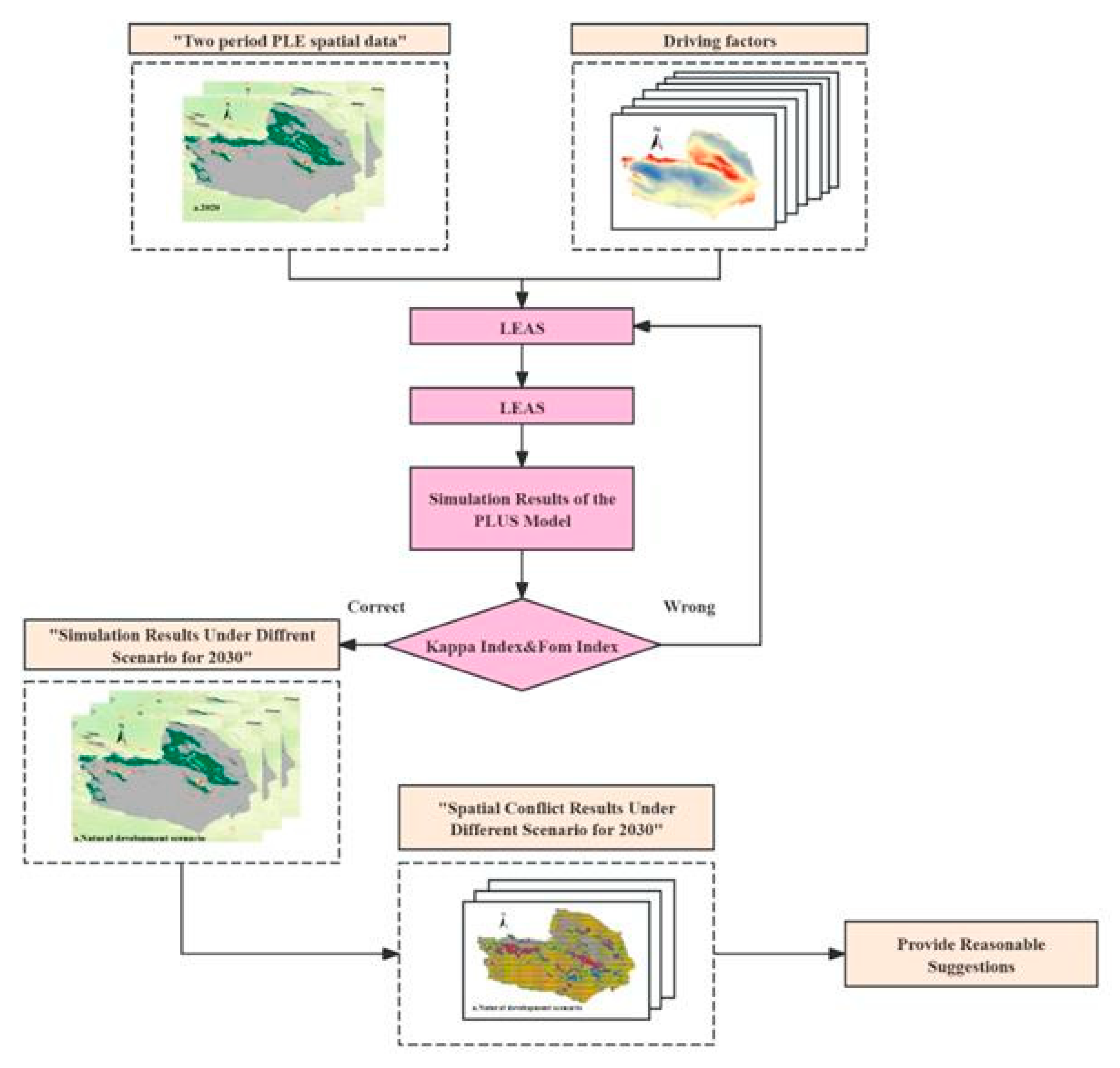
3. Research Methods
3.1. Classification of “Production–Living–Ecological” (PLE) Space
3.2. Construction of the PLECs Measurement Model
- (1)
- Complexity index
- (2)
- Vulnerability index
- (3)
- Stability index
3.3. Subdivision of Evaluation Units
3.4. Geographically Weighted Regression Model
3.5. PLUS Model
3.5.1. Multi-Scenario Simulation of PLE Space
3.5.2. Parameter Settings
- (1)
- Restricted Conversion Area Settings
- (2)
- Land Demand Parameter Settings
- (3)
- Neighborhood Weight Parameter Settings
- (4)
- Transition Matrix Parameter Settings
3.5.3. PLUS Model Multi-Scenario Forecasting Settings
4. Results
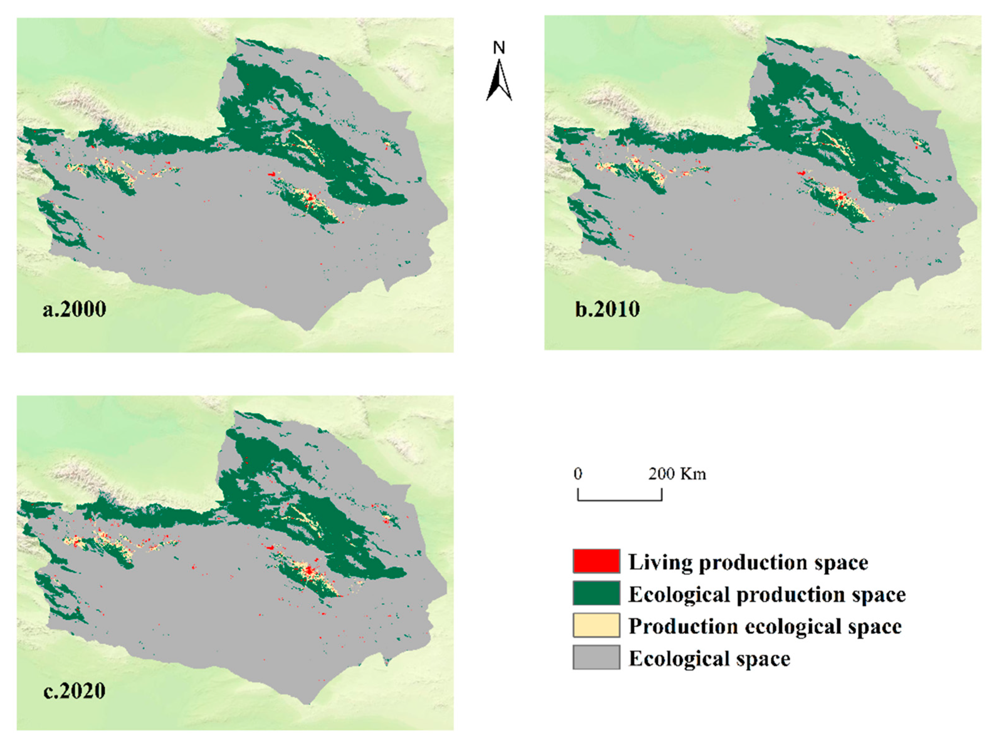
4.1. Changes in the PLE Space Pattern
4.2. PLEC Change Analysis
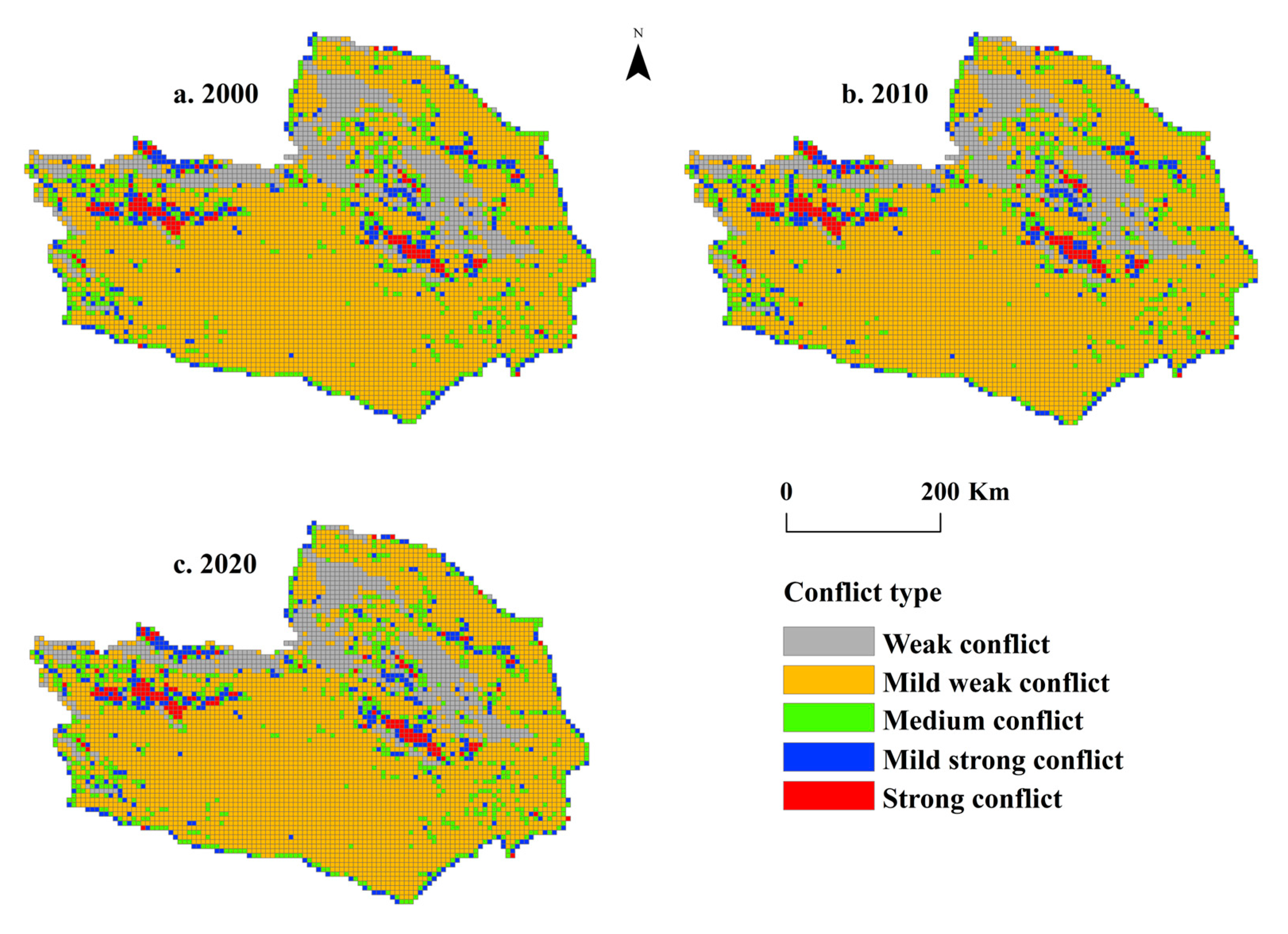
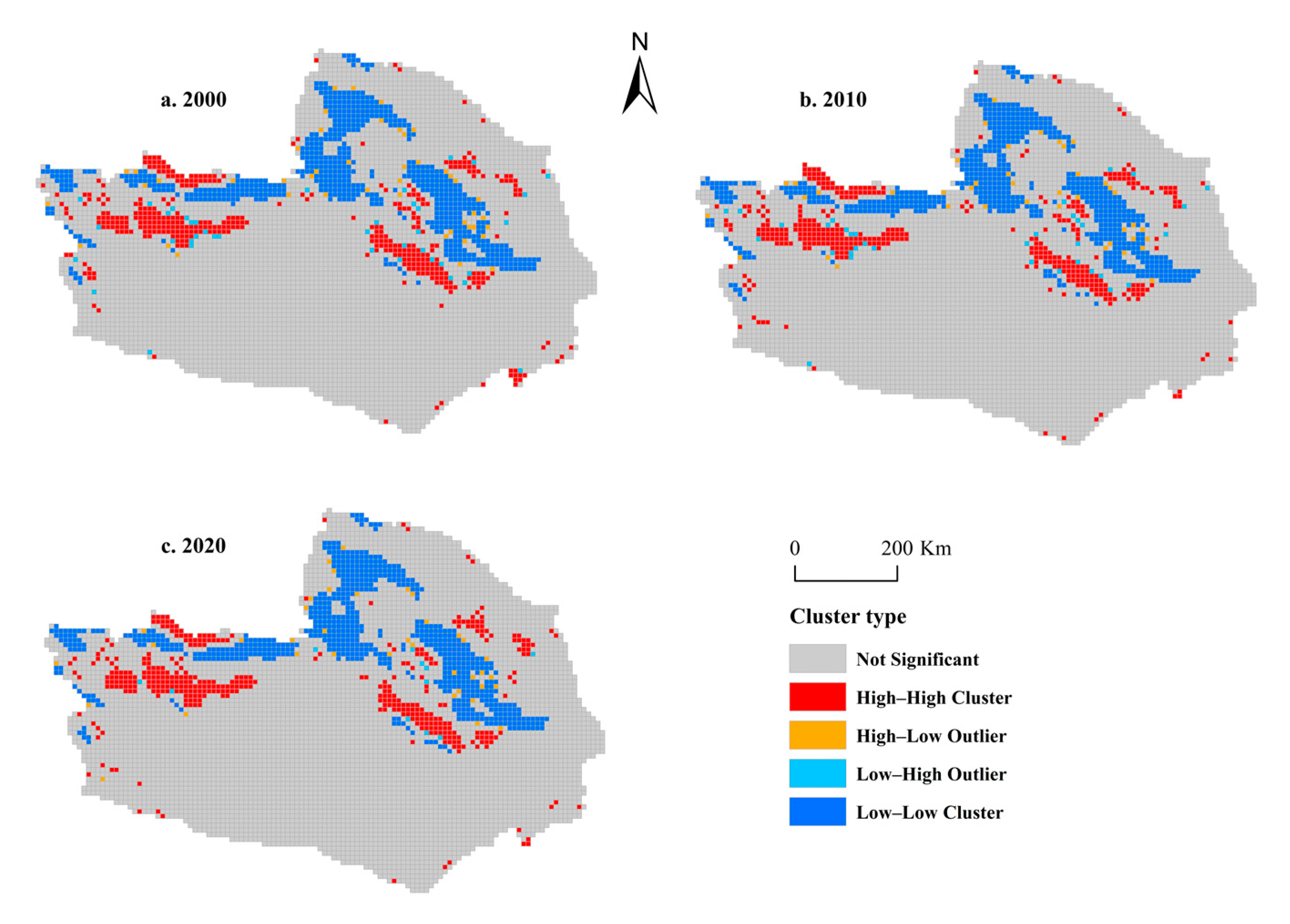
4.3. Spatial Clustering Characteristics of PLECs in the Study Area
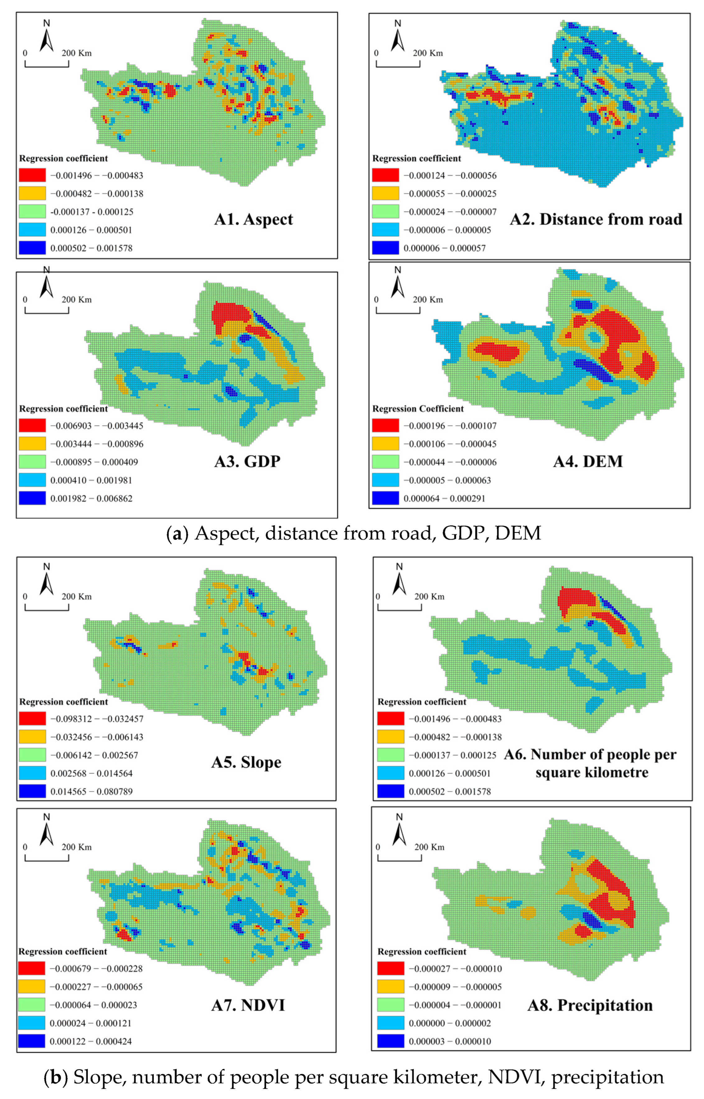
4.4. Geographically Weighted Regression (GWR) Model
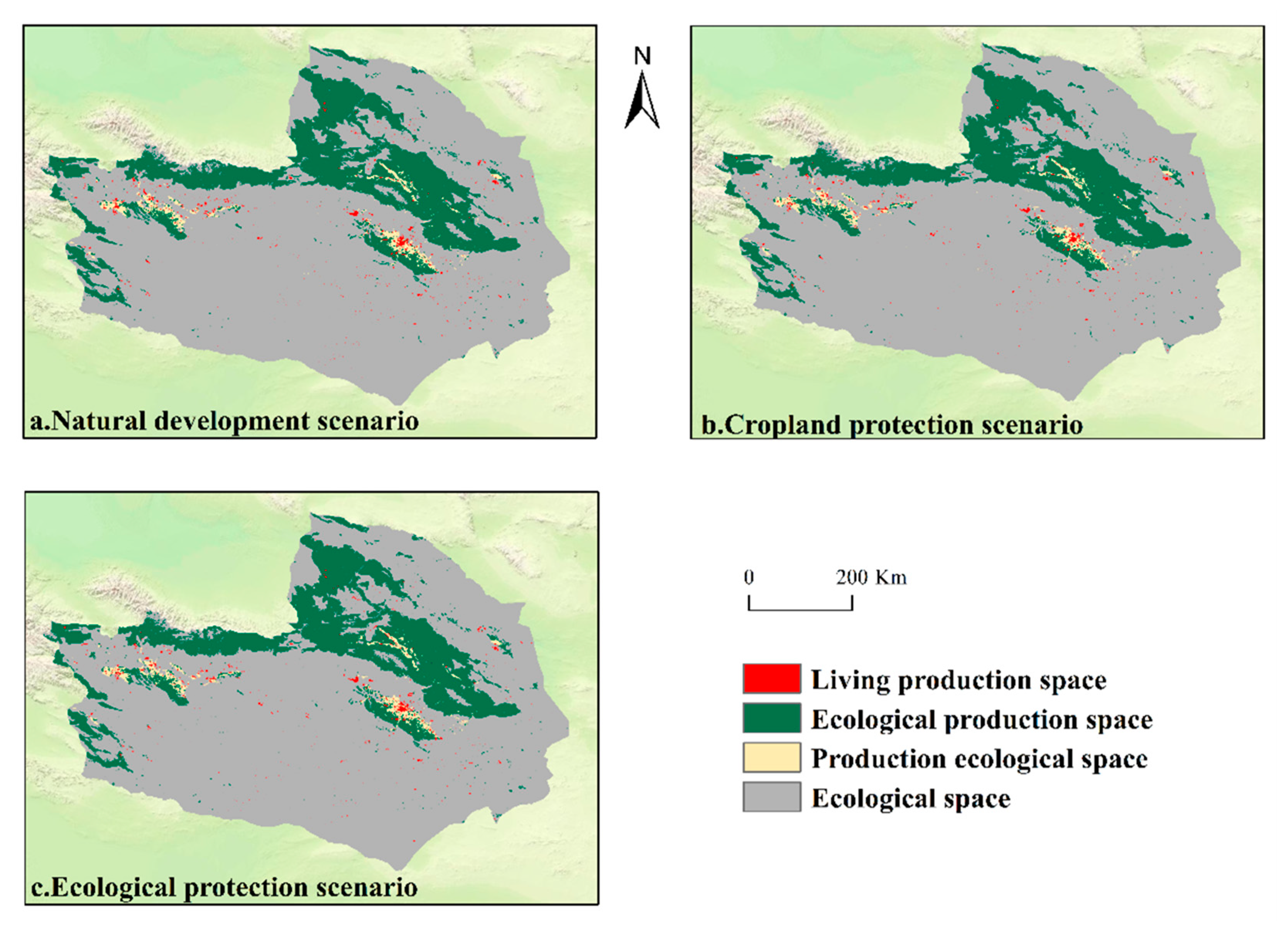
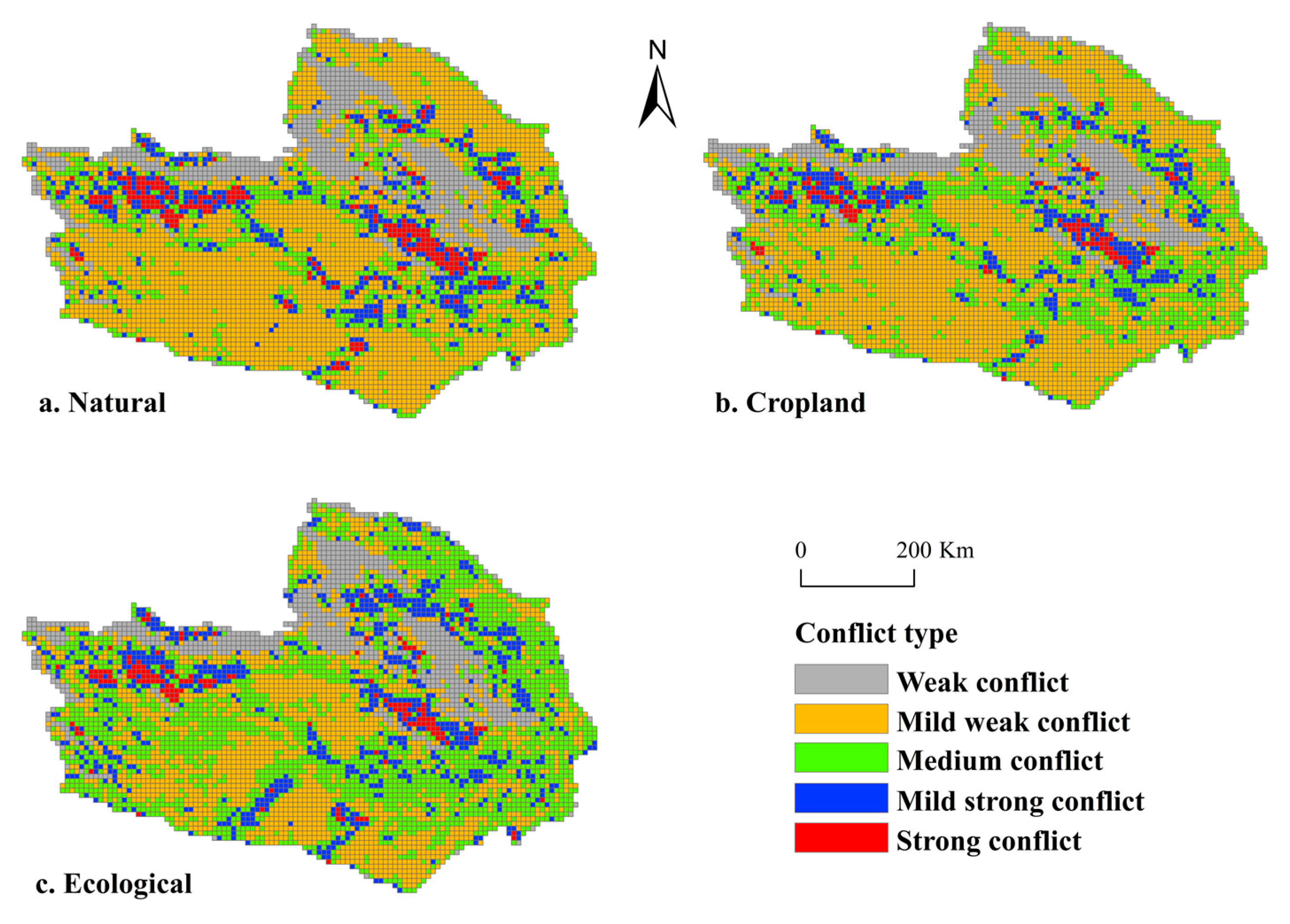
4.5. PLECs Pattern Multi-Scenario Simulation
5. Discussion
5.1. Identification of PLECs
5.2. Key Factors Influencing PLECs
5.3. Optimal Allocation Scheme for PLE Spaces
5.4. Strategic Recommendations
5.5. Limitations of the Study
6. Conclusions
- (1)
- From 2000 to 2020, the area of ecological space in the study area was the largest, accounting for 79% of the total area, followed by ecological–production space, production–ecological space, and living–production space.
- (2)
- From 2000 to 2020, the conflict level in the study area was predominantly mild weak conflict, with strong conflicts initially increasing and then decreasing. Medium and mild strong conflicts continued to grow, while weak conflicts consistently decreased.
- (3)
- The spatial conflict distribution in the study area from 2000 to 2020 shows a significant positive correlation. Analysis of the local spatial autocorrelation clustering map and the results from the GWR driving factors indicates that high–high clustering areas are mainly located in the built-up areas of Gaochang District, Toksun County, Shanshan County, and Yizhou District, along with their surrounding areas, with slight expansion. Low–low clustering areas are distributed across most regions of the Tianshan Mountains and the northern part of Barkol Kazak Autonomous County. Areas with non-significant clustering are primarily ecological spaces, which also intersect with other spatial types. Factors such as NDVI, GDP, population, and distance to roads have a positive impact on PLECs, while factors such as elevation, slope, direction, and precipitation exhibit inhibitory effects.
- (4)
- In the cropland protection scenario under different development contexts, the spatial conflict level in the study area is the lowest, with weak and moderate conflict zones accounting for 75.5%. This scenario is considered the optimal direction for future regional development. The regulation of land use conflicts in the region should adhere to the principle of maximizing overall regional benefits, with the goal of improving the overall welfare of regional development. Additionally, it is crucial to formulate a targeted and multidimensional land use management policy system based on national and regional policies.
Author Contributions
Funding
Data Availability Statement
Conflicts of Interest
References
- Sun, Y. Impact of humanactivities on climate system: An interpretation of Chapter Ⅲ of WGⅠ report of IPCC AR6. Trans. Atmos. Sci. 2021, 44, 654–657. [Google Scholar]
- D’Odorico, P.; Bhattachan, A.; Davis, K.F.; Ravi, S.; Runyan, C.W. Global desertification: Drivers and feedbacks. Adv. Water Resour. 2013, 51, 326–344. [Google Scholar] [CrossRef]
- Huang, J.P.; Yu, H.P.; Guan, X.D.; Wang, G.; Guo, R. Accelerated dryland expansion under climate change. Nat. Clim. Change 2016, 6, 166–171. [Google Scholar] [CrossRef]
- Reynolds, J.F.; Stafford Smith, D.M.; Lambin, E.F.; Turner, B.L.; Mortimore, M.; Batterbury, S.P.; Downing, T.E.; Dowlatabadi, H.; Fernández, R.J.; Herrick, J.E.; et al. Global desertification:: Building a science for dryland development. Science 2007, 316, 847–851. [Google Scholar] [CrossRef]
- Yang, Q.; Duan, X.; Wang, L.; Jin, Z.F. Land Use Transformation Based on Ecological-production-living Spaces and Associated Eco-environment Effects: A Case Study in the Yangtze River Delta. Sci. Geogr. Sin. 2018, 38, 97–106. [Google Scholar]
- Fang, C.; Bao, C.; Zhang, C. Analysis on the changing condition and the evolutive scene of the ecology-production-living carrying capacity in arid area: A case study in Yuli District in the Lower Reaches of Tarim River. Acta Ecol. Sin. 2003, 23, 1915–1923. [Google Scholar]
- Zhang, L.; Hou, Q.; Duan, Y. A literature review on Production-Living-Ecological Spaces in the context of ecological civilization: Connotation, problems and countermeasures. Acta Ecol. Sin. 2024, 44, 47–59. [Google Scholar]
- Li, G.; Fang, C. Quantitative function identification and analysis of urban ecological-production-living spaces. Acta Geogr. Sin. 2016, 71, 49–65. [Google Scholar]
- Zhang, H.; Xu, E.; Zhu, H. An ecological-living-industrial land classification system and its spatial distribution in China. Resour. Sci. 2015, 37, 1332–1338. [Google Scholar]
- Liu, J.; Liu, Y.; Li, Y. Classification evaluation and spatial-temporal analysis of “production-living-ecological” spaces in China. Acta Geogr. Sin. 2017, 72, 1290–1304. [Google Scholar]
- Dai, W.; Jiang, F.; Huang, W.; Liao, L.H.; Jiang, K. Study on Transition of Land Use Function and Ecosystem Service Value Based on the Conception of Production, Living and Ecological Space: A Case Study of the Fuzhou New Area. J. Nat. Resour. 2018, 33, 2098–2109. [Google Scholar]
- Wang, K.; Yao, Y.; Bao, J. Dynamic Change of Ecological-living-industrial Land and Its Spatial Agglomeration at County-scale. Bull. Soil Water Conserv. 2018, 38, 306–312. [Google Scholar]
- Long, H.; Tu, S. Rural restructuring: Theory, approach and research prospect. Acta Geogr. Sin. 2017, 72, 563–576. [Google Scholar]
- Liu, P.; Chen, R.; Yang, C. Study on Layout Optimization of Rural Settlements Based on Coordination of Production, Living and Ecology Space. Res. Soil Water Conserv. 2017, 24, 283–288. [Google Scholar]
- Huang, T.; Zhang, Y. Transformation of land use function and response of eco-environment based on production-life-ecology space: A case study of resource-rich area in western Guangxi. Acta Ecol. Sin. 2021, 41, 348–359. [Google Scholar]
- Alston, L.J.; Libecap, G.D.; Mueller, B. Land reform policies, the sources of violent conflict, and implications for deforestation in the Brazilian Amazon. J. Environ. Econ. Manag. 2000, 39, 162–188. [Google Scholar] [CrossRef]
- Von Der Dunk, A.; Grêt-Regamey, A.; Dalang, T.; Hersperger, A.M. Defining a typology of peri-urban land-use conflicts–A case study from Switzerland. Landsc. Urban Plan. 2011, 101, 149–156. [Google Scholar] [CrossRef]
- Brown, G.; Raymond, C.M. Methods for identifying land use conflict potential using participatory mapping. Landsc. Urban Plan. 2014, 122, 196–208. [Google Scholar] [CrossRef]
- Delgado-Matas, C.; Mola-Yudego, B.; Gritten, D.; Kiala-Kalusinga, D.; Pukkala, T. Land use evolution and management under recurrent conflict conditions: Umbundu agroforestry system in the Angolan Highlands. Land Use Policy 2015, 42, 460–470. [Google Scholar] [CrossRef]
- Andrew, J.S. Potential application of mediation to land use conflicts in small-scale mining. J. Clean. Prod. 2003, 11, 117–130. [Google Scholar] [CrossRef]
- Bohua, Y.U.; Changhe, L.V. The Progress and Prospect of Land Use Conflicts. Prog. Geogr. 2006, 25, 106–115. [Google Scholar]
- Zhou, G.; Peng, J. The Connotation Analysis of Spatial Conflict in Fast Urbanization Regions: A Case Study of Changsha-Zhuzhou-Xiangtan Urban Agglomeration. Prog. Geogr. 2012, 31, 717–723. [Google Scholar]
- Liu, S. Spatial Patterns and Dynamic Mechanisms of Urban Land Use Growth. Prog. Geogr. 2002, 21, 43–50. [Google Scholar]
- Chen, L.T.; Cai, H.S. Study on land use conflict identification and territorial spatial zoning control in Rao River Basin, Jiangxi Province, China. Ecol. Indic. 2022, 145, 109594. [Google Scholar] [CrossRef]
- Peng, Y.; Wang, J.; Wang, S.; Tian, L.; Liu, J.; Wu, Z. Spatiotemporal pattern evolution of land use conflict in Urumqi City from the perspective of ecological security. Arid. Land Geogr. 2024, 47, 81–92. [Google Scholar]
- Liao, L.; Dai, W.; Chen, J.; Huang, W.; Jiang, F.; Hu, Q. Spatial conflict between ecological-production-living spaces on Pingtan Island during rapid urbanization. Resour. Sci. 2017, 39, 1823–1833. [Google Scholar]
- He, Y.; Tang, C.; Zhou, G.; He, S.; Qiu, Y.H.; Shi, L.; Zhang, H.Z. The Analysis of Spatial Conflict Measurement in Fast Urbanization Region from the Perspective of Geography A Case Study of Changsha-Zhuzhou-Xiangtan Urban Agglomeration. J. Nat. Resour. 2014, 29, 1660–1674. [Google Scholar]
- Zhao, X.; Tang, F.; Zhang, P.; Hu, B.; Xu, L. Dynamic simulation and characteristic analysis of county production-livingecological spatial conflicts based on CLUE-S model. Acta Ecol. Sin. 2019, 39, 5897–5908. [Google Scholar]
- Reyes-García, V.; Orta-Martínez, M.; Gueze, M.; Luz, A.C.; Paneque-Gálvez, J.; Macía, M.J.; Pino, J. Does participatory mapping increase conflicts? A randomized evaluation in the Bolivian Amazon. Appl. Geogr. 2012, 34, 650–658. [Google Scholar] [CrossRef]
- Hong, K.R.; Zou, Y.C.; Zhu, M.Y.; Zhang, Y. A Game Analysis of Farmland Expropriation Conflict in China under Multi-Dimensional Preference: Cooperation or Resistance? Land 2021, 10, 124. [Google Scholar] [CrossRef]
- Yang, Y.; An, Q.; Zhu, L. Diagnosis Based on the PSR Model of Rural Land-use Conflicts Intensity. Prog. Geogr. 2012, 31, 1552–1560. [Google Scholar]
- Zhou, D.; Xu, J.; Wang, L. Land use spatial conflicts and complexity: A case study of the urban agglomeration around Hangzhou Bay, China. Geogr. Res. 2015, 34, 1630–1642. [Google Scholar]
- Meng, J.; Jiang, S.; Laba, Z.; Zhang, W. The Spatial and Temporal Analysis of Land Use Conflict in the Middle Reaches of the Heihe River Based on Landscape Pattern. Sci. Geogr. Sin. 2020, 40, 1553–1562. [Google Scholar]
- Ma, W.; Jiang, G.; Chen, Y.; Qu, Y.; Zhou, T.; Li, W. How feasible is regional integration for reconciling land use conflicts across the urban–rural interface? Evidence from Beijing–Tianjin–Hebei metropolitan region in China. Land Use Policy 2020, 92, 104433. [Google Scholar] [CrossRef]
- Wang, C.; Wu, J.H.; Li, M.; Huang, X.; Lei, C.; Wang, H. Evaluation of spatial conflicts of land use and its driving factors in arid and semiarid regions: A case study of Xinjiang, China. Ecol. Indic. 2024, 166, 112483. [Google Scholar] [CrossRef]
- Zhou, D.; Lin, Z.L.; Lim, S.H. Spatial characteristics and risk factor identification for land use spatial conflicts in a rapid urbanization region in China. Environ. Monit. Assess. 2019, 191, 677. [Google Scholar] [CrossRef]
- Zhang, H.; Lou, Q. Study on spatial structure of greenland in urban fringe area of Guangzhou based on game theory:a case study of Panyu district. Ecol. Environ. Sci. 2010, 19, 1593–1598. [Google Scholar]
- Chen, S.; Ai, D.; Fu, Y. Spatial conflict measurement and influencing factors based on ecological security: A case study of Kunming City. J. China Agric. Univ. 2020, 25, 141–150. [Google Scholar]
- Peng, J.; Zhou, G.; Tang, C.; He, Y. The Analysis of Spatial Conflict Measurement in Fast Urbanization Region Based on Ecological SecurityA Case Study of Changsha-Zhuzhou-Xiangtan Urban Agglomeration. J. Nat. Resour. 2012, 27, 1507–1519. [Google Scholar]
- Lu, S.; Zhang, J.; Wu, Z. Study on the Spatial Conflict of Land Use in Jinghe County Oasis. J. Ecol. Rural. Environ. 2022, 38, 428–436. [Google Scholar]
- Pan, F.; Wan, Q.; Zeng, J.; Wang, H.; Huang, Q. Evolution Characteristics and Influence Factors of Spatial Conflicts Between Production-Living-Ecological Space in the Rapid Urbanization Process of Hubei Province, China. Econ. Geogr. 2023, 43, 80–92. [Google Scholar]
- Zeng, C.F.; He, J.; He, Q.Q.; Mao, Y.; Yu, B. Assessment of Land Use Pattern and Landscape Ecological Risk in the Chengdu-Chongqing Economic Circle, Southwestern China. Land 2022, 11, 659. [Google Scholar] [CrossRef]
- Brunsdon, C.; Fotheringham, S.; Charlton, M. Geographically weighted regression. J. R. Stat. Soc. 1998, 47, 431–443. [Google Scholar] [CrossRef]
- Lv, J.J.; Wang, Y.F.; Liang, X.; Yao, Y.; Ma, T.; Guan, Q. Simulating urban expansion by incorporating an integrated gravitational field model into a demand-driven random forest-cellular automata model. Cities 2021, 109, 103044. [Google Scholar] [CrossRef]
- Li, J.Y.; Chen, X.; Kurban, A.; Van de Voorde, T.; De Maeyer, P.; Zhang, C. Coupled SSPs-RCPs scenarios to project the future dynamic variations of water-soil-carbon-biodiversity services in Central Asia. Ecol. Indic. 2021, 129, 107936. [Google Scholar] [CrossRef]
- Fang, Z.; Ding, T.; Chen, J.; Xue, S.; Zhou, Q.; Wang, Y.; Wang, Y.; Huang, Z.; Yang, S. Impacts of land use/land cover changes on ecosystem services in ecologically fragile regions. Sci. Total Environ. 2022, 831, 154967. [Google Scholar] [CrossRef]
- Zhou, M.; Wang, C. Multi-scenario simulation of “production-livelihood-ecological”space in Urumqi based on PLUS. China Environ. Sci. 2024, 44, 4021–4030. [Google Scholar]
- Huang, K.; Dai, W.; Huang, W.; Ou, H.; Hu, H. Impacts of Land Use Change Evaluation on Habitat Quality Based on CA-Markov and InVEST Models Taking Fuzhou New District of Fujian Province as an Example. Bull. Soil Water Conserv. 2019, 39, 155–162. [Google Scholar]
- Yahefujiang, H.; Zou, J.; Ding, J.L.; Zou, W.; Tangjialeke, W.; Yang, M. Spatial and Temporal Variation in Water Use Efficiency and Ecosystem Photosynthetic Efficiency in Central Asia. Remote Sens. 2023, 15, 5240. [Google Scholar] [CrossRef]
- Dong, Z.; Yuan, Q.; Wang, Z.; Ren, P. Analysis and simulation prediction of the evolutionary characteristics of the living-production-ecological spatial conflicts in the agriculture-pastoral ecotone in western Sichuan:Taking four counties in Aba Prefecture as examples. Acta Ecol. Sin. 2023, 43, 6243–6256. [Google Scholar]
- Wang, Z.; Zhang, J.; Li, H.; Su, W. Multi-scale spatio-temporal evolution and multi-scenario simulation of land use conflict in Chongqing. Acta Ecol. Sin. 2024, 44, 1024–1039. [Google Scholar]
- Hu, Y.; An, R.; Yang, J.; Liu, Y. Measurement and Driving Mechanism of Land Use Conflict Based on Landscape Pattern—A Case Study of Wuhan Metropolitan Area. Res. Soil Water Conserv. 2024, 31, 354–364. [Google Scholar]
- Wang, B.; Shu, X.; Liao, F.; Li, Y.; Wan, Z. Spatitemporal of Land Use Conflicts and Multi-Scenario Simulation in Poyang Lake Area Based on Optimal Landscape Scale. Res. Soil Water Conserv. 2024, 31, 336–347. [Google Scholar]
- Zou, L.L.; Liu, Y.S.; Wang, J.Y.; Yang, Y. An analysis of land use conflict potentials based on ecological-production-living function in the southeast coastal area of China. Ecol. Indic. 2021, 122, 107297. [Google Scholar] [CrossRef]
- Yuan, S.F.; Mei, Z.H.; Zhu, C.M.; Cao, R.; Li, S.; Yang, L.; Su, Y.; Li, W. Investigating the spatio-temporal interactive relationship between land use structure and ecosystem services in urbanizing China. Ecol. Indic. 2024, 158, 111315. [Google Scholar] [CrossRef]
- Wang, Z.Y.; Deng, W.; Zhang, S.Y.; Zhang, H. Improved trade-off model of land use functions: Differentiated objective setting by territory spatial planning. Ecol. Indic. 2024, 160, 111881. [Google Scholar] [CrossRef]
- Feng, Y.; Zhai, S.; Jiang, X.; Luo, J.; Yan, P.; Dong, C.; Han, J. Simulating spatio-temporal pattern of production-living-ecological space and evaluating eco-environmental effects in Zhongyuan Urban Agglomeration based on FLUS model and shared socioeconomic pathways. Acta Ecol. Sin. 2023, 43, 8292–8308. [Google Scholar]
- Bao, W.K.; Yang, Y.Y.; Zou, L.L. How to reconcile land use conflicts in mega urban agglomeration? A scenario-based study in the Beijing-Tianjin-Hebei region, China. J. Environ. Manag. 2021, 296, 113168. [Google Scholar] [CrossRef]
- Zhou, C.; Jin, W.; Zhang, G.; Li, M.; Wang, S. Spatio-temporal characteristics and influencing factors of state owned construction land supply in China. Acta Geogr. Sin. 2019, 74, 16–31. [Google Scholar]
- Pacione, M. Private profit, public interest and land use planning-A conflict interpretation of residential development pressure in Glasgow’s rural-urban fringe. Land Use Policy 2013, 32, 61–77. [Google Scholar] [CrossRef]
- Zhu, X.; Zhang, Q.; Sun, P. Effects of urbanization on spatio-temporal distribution of precipitations in Beijing and its related causes. Acta Geogr. Sin. 2018, 73, 2086–2104. [Google Scholar]
- Kiem, A.S.; Johnson, F.; Westra, S.; van Dijk, A.; Evans, J.P.; O’donnell, A.; Rouillard, A.; Barr, C.; Tyler, J.; Thyer, M.; et al. Natural hazards in Australia: Droughts. Clim. Change 2016, 139, 37–54. [Google Scholar] [CrossRef]
- Tangjialeke, W.; Zou, J.; Ding, J.L.; Yahefujiang, H.; Huang, S.; Li, J. Analysis of drought response thresholds and drought-causing factors of central Asian vegetation. Ecol. Indic. 2024, 169, 112926. [Google Scholar] [CrossRef]
- Yu, A.T.W.; Wu, Y.Z.; Zheng, B.B.; Zhang, X.; Shen, L. Identifying risk factors of urban-rural conflict in urbanization: A case of China. Habitat Int. 2014, 44, 177–185. [Google Scholar] [CrossRef]
- Zong, S.S.; Hu, Y.C.; Bai, Y.P.; Guo, Z.; Wang, J. Analysis of the distribution characteristics and driving factors of land use conflict potentials in the Bohai Rim coastal zone. Ocean Coast. Manag. 2022, 226, 106260. [Google Scholar] [CrossRef]
- Wang, C.; Wang, H.W.; Wu, J.H.; He, X.; Luo, K.; Yi, S. Identifying and warning against spatial conflicts of land use from an ecological environment perspective: A case study of the Ili River Valley, China. J. Environ. Manag. 2024, 351, 119757. [Google Scholar] [CrossRef]
- Jiang, L.; Deng, X.Z.; Seto, K.C. The impact of urban expansion on agricultural land use intensity in China. Land Use Policy 2013, 35, 33–39. [Google Scholar] [CrossRef]
- Gomez-Vazquez, I.; Alvarez-Alvarez, P.; Marey-Pérez, M.F. Conflicts as enhancers or barriers to the management of privately owned common land: A method to analyze the role of conflicts on a regional basis. For. Policy Econ. 2009, 11, 617–627. [Google Scholar]
- Wang, Y.; Li, W.; Zeng, X.; Li, P.; Xue, B. The Spatial Multi-scale Mechanism of Land Use Elemental Conflicts in Shenyang Economic Zone. Econ. Geogr. 2022, 42, 231–239. [Google Scholar]
- Zou, Y.; Meng, J.J.; Zhu, L.K.; Han, Z.; Ma, Y. Characterizing land use transition in China by accounting for the conflicts underlying land use structure and function. J. Environ. Manag. 2024, 349, 119311. [Google Scholar] [CrossRef]
- Zinda, J.A.; Trac, C.J.; Zhai, D.; Harrell, S. Dual-function forests in the returning farmland to forest program and the flexibility of environmental policy in China. Geoforum 2017, 78, 119–132. [Google Scholar] [CrossRef]
- Zheng, F.Y.; Hu, Y.C.; Zuo, Y.Q. Did the ecological engineering have a great impact on the land use change? Environ. Monit. Assess. 2018, 190, 690. [Google Scholar] [CrossRef] [PubMed]
- Han, X.J.; Wang, P.; Wang, J.J.; Qiao, M.; Zhao, X. Evaluation of human-environment system vulnerability for sustainable development in the Liupan mountainous region of Ningxia, China. Environ. Dev. 2020, 34, 100525. [Google Scholar] [CrossRef]
- Xiao, L.; Liu, Q.; Yu, H.; Lin, M.S. Community regulation in national park based on land use conflict identification:A case study on Qianjiangyuan National Park. Acta Ecol. Sin. 2020, 40, 7277–7286. [Google Scholar]

| Category | Data | Year | Original Resolution | Data Resource |
|---|---|---|---|---|
| Land use data | 2000, 2010, 2020 | 30 m | http://www.resdc.cn (accessed on 18 November 2024) | |
| Socioeconomic driver | GDP | 2022 | 1000 m | |
| Population | 2022 | 1000 m | ||
| Distance from road | 2022 | 30 m | www.Webmap.cn (accessed on 18 November 2024) | |
| Distance from the railway | ||||
| Natural driver | Digital Elevation Model (DEM) Slope | 2020 | 30 m | http://www.gscloud.cn (accessed on 18 November 2024) |
| Aspect | ||||
| Soil type | 1995 | 1000 m | http://www.resdc.cn (accessed on 18 November 2024) | |
| NDVI | 2020 | 30 m | ||
| Annual precipitation | 2020 | 1000 m | WorldClimv2.1 (www.worldclim.org/) (accessed on 18 November 2024) |
| PLES Classification | Meaning | Corresponding Land Use Types |
|---|---|---|
| Living–production space | Primarily meets basic human living and spiritual needs while also having diverse production functions, with the highest economic value. | Urban Land, Rural Residential Areas, Industrial and Transportation Construction Land |
| Ecological–production space | Primarily focused on ecological functions, while allowing for appropriate production activities to provide economic benefits. | Grassland, Forest Land, Reservoirs and Ponds |
| Production–ecological space | Primarily focused on agricultural production functions, while also serving ecological functions. | Paddy Fields, Dry Farmland |
| Ecological space | Provides ecological products and services, with functions such as climate regulation, carbon sequestration and oxygen release, and biodiversity protection. | Unused Land, Rivers and Canals, Lakes, Glaciers and Permanent Snow, Tidal Flats Beach Land |
| Conflict Type | Threshold Interval | Space Landscape Patch Performance |
|---|---|---|
| Weak spatial conflict | (0, 0.15] | Considered to be minimally disturbed, with a complete landscape patch structure and high stability |
| Mild weak spatial conflict | (0.15, 0.32] | Intersecting with areas of weak spatial conflict |
| Medium spatial conflict | (0.32, 0.43] | The fragmentation of landscape patches increases, with complex patch boundaries. |
| Mild strong spatial conflict | (0.43, 0.60] | The fragmentation, vulnerability, and complexity of landscape patches increase |
| Strong spatial conflict | (0.60, 1] | Landscape patches are fragmented and isolated, with complex structures and high fragmentation levels. |
| Space Type | Weights |
|---|---|
| Living production space | 1 |
| Ecological production space | 0.3 |
| Production ecological space | 0.5 |
| Ecological space | 0.4 |
| Type | ND Scenario | CP Scenario | EP Scenario | |||||||||
|---|---|---|---|---|---|---|---|---|---|---|---|---|
| LP | EP | PE | E | LP | EP | PE | E | LP | EP | PE | E | |
| LP | 1 | 1 | 1 | 1 | 1 | 1 | 1 | 1 | 1 | 1 | 1 | 1 |
| EP | 1 | 1 | 1 | 1 | 1 | 1 | 1 | 1 | 0 | 1 | 0 | 0 |
| PE | 1 | 1 | 1 | 1 | 0 | 0 | 1 | 0 | 1 | 1 | 1 | 1 |
| E | 1 | 1 | 1 | 1 | 1 | 1 | 1 | 1 | 1 | 1 | 1 | 1 |
| Space Type | 2000 | 2010 | 2020 | |||
|---|---|---|---|---|---|---|
| Area/km2 | Proportion/% | Area/km2 | Proportion/% | Area/km2 | Proportion/% | |
| LP | 522.383 | 0.25 | 556.022 | 0.27 | 977.337 | 0.47 |
| EP | 39,396.8 | 19.04 | 39,152.1 | 18.92 | 39,126.5 | 18.91 |
| PE | 2691.02 | 1.30 | 3076 | 1.49 | 3053.33 | 1.48 |
| E | 164,336 | 79.41 | 164,162 | 79.33 | 163,785 | 79.15 |
| Total | 206,946.2 | 100.00 | 206,946.2 | 100 | 206,942.2 | 100 |
| Conflict Type | Conflict Classification | Number of Spatial Conflict Units | Proportion of Conflict Units (%) | ||||
|---|---|---|---|---|---|---|---|
| 2000 | 2010 | 2020 | 2000 | 2010 | 2020 | ||
| Weak spatial conflict | (0, 0.15] | 709 | 696 | 711 | 11.82 | 11.61 | 11.86 |
| Mild weak spatial conflict | (0.15, 0.32] | 4112 | 4060 | 3691 | 68.58 | 67.71 | 66.06 |
| Medium spatial conflict | (0.32, 0.43] | 694 | 699 | 793 | 11.57 | 11.66 | 13.23 |
| Mild strong spatial conflict | (0.43, 0.60] | 360 | 384 | 393 | 6 | 6.40 | 6.55 |
| Strong spatial conflict | (0.60, 1] | 118 | 154 | 135 | 1.97 | 2.57 | 2.25 |
| Total | 5996 | 5996 | 5996 | 100 | 100 | 100 | |
| Factors | R2 | R2 Adjusted | Regression Coefficient |
|---|---|---|---|
| NDVI | 0.76 | 0.67 | 0.00132 |
| DEM | 0.41 | 0.38 | −1.8848 |
| GDP | 0.58 | 0.54 | 0.01297 |
| POP | 0.57 | 0.53 | 0.00256 |
| Aspect | 0.73 | 0.62 | −1.7135 |
| Road | 0.77 | 0.68 | 0.08904 |
| Slope | 0.73 | 0.63 | −0.00272 |
| Precipitation | 0.38 | 0.36 | −0.00027 |
| Conflict Type | Conflict Classification | 2020 (%) | ND (%) | cp (%) | EP (%) |
|---|---|---|---|---|---|
| Weak spatial conflict | (0, 0.15] | 11.86 | 12.06 | 12.88 | 11.86 |
| Mild weak spatial conflict | (0.15, 0.32] | 66.06 | 52.69 | 48.15 | 32.10 |
| Medium spatial conflict | (0.32, 0.43] | 13.23 | 20.06 | 27.35 | 39.44 |
| Mild strong spatial conflict | (0.43, 0.60] | 6.55 | 10.67 | 9.31 | 13.98 |
| Strong spatial conflict | (0.60, 1] | 2.25 | 4.52 | 2.32 | 2.62 |
| Total | 100 | 100 | 100 | 100 |
Disclaimer/Publisher’s Note: The statements, opinions and data contained in all publications are solely those of the individual author(s) and contributor(s) and not of MDPI and/or the editor(s). MDPI and/or the editor(s) disclaim responsibility for any injury to people or property resulting from any ideas, methods, instructions or products referred to in the content. |
© 2025 by the authors. Licensee MDPI, Basel, Switzerland. This article is an open access article distributed under the terms and conditions of the Creative Commons Attribution (CC BY) license (https://creativecommons.org/licenses/by/4.0/).
Share and Cite
Yerkenhazi, A.; Mamat, K.; Abulizi, A.; Mamitimin, Y.; Wei, X.; Tang, S.; Wang, J.; Bai, S.; Yuan, L. Identification of Production–Living–Ecological Spatial Conflicts and Multi-Scenario Simulations in Extreme Arid Areas. Land 2025, 14, 1002. https://doi.org/10.3390/land14051002
Yerkenhazi A, Mamat K, Abulizi A, Mamitimin Y, Wei X, Tang S, Wang J, Bai S, Yuan L. Identification of Production–Living–Ecological Spatial Conflicts and Multi-Scenario Simulations in Extreme Arid Areas. Land. 2025; 14(5):1002. https://doi.org/10.3390/land14051002
Chicago/Turabian StyleYerkenhazi, Amanzhuli, Kerim Mamat, Abudukeyimu Abulizi, Yusuyunjiang Mamitimin, Xuemei Wei, Shanshan Tang, Junxia Wang, Shaojie Bai, and Le Yuan. 2025. "Identification of Production–Living–Ecological Spatial Conflicts and Multi-Scenario Simulations in Extreme Arid Areas" Land 14, no. 5: 1002. https://doi.org/10.3390/land14051002
APA StyleYerkenhazi, A., Mamat, K., Abulizi, A., Mamitimin, Y., Wei, X., Tang, S., Wang, J., Bai, S., & Yuan, L. (2025). Identification of Production–Living–Ecological Spatial Conflicts and Multi-Scenario Simulations in Extreme Arid Areas. Land, 14(5), 1002. https://doi.org/10.3390/land14051002