Article

Simulation Analysis of Land Use Change via the PLUS-GMOP Coupling Model

1
School of Public Administration, China University of Geosciences (Wuhan), Wuhan 430074, China
2
Ningxia Natural Resources Information Center, Yinchuan 750002, China
3
Tibet Datang International Upper Nujiang River Hydropower Development Co., Ltd., Lhasa 850001, China
4
State Key Laboratory of Information Engineering in Surveying Mapping and Remote Sensing, Wuhan University, Wuhan 430079, China
5
School of Earth Science and Engineering, Southwest Jiaotong University, Chengdu 610097, China
6
School of Water and Environment, Chang’an University, Xi’an 710054, China
7
Key Laboratory of Subsurface Hydrology and Ecological Effects in Arid Region, Ministry of Education, Chang’an University, Xi’an 710054, China
*
Author to whom correspondence should be addressed.
Land 2025, 14(4), 802; https://doi.org/10.3390/land14040802
Submission received: 28 January 2025 / Revised: 27 March 2025 / Accepted: 1 April 2025 / Published: 8 April 2025

Abstract

:
It is crucial to simulate land use change and assess the corresponding impact on ecosystem services to develop informed land management policies and conservation strategies. To comprehensively simulate the patterns of land use change under different management policies and evaluate the corresponding ecological service values (ESV), a method for coupling the Generalized Multi-Objective Programming (GMOP) model and Patch-generating Land Use Simulation (PLUS) model is proposed in this study. First, the GMOP model is used to obtain optimized land use solutions under different scenarios. Then, the PLUS model is used to analyze the mechanism driving land expansion, explore land conversion patterns, and, ultimately, achieve spatial expression of land use quantity changes. The uncertain parameters in the coupled model are processed by intuitionistic fuzzy numbers. The coupled model successfully integrates the outstanding spatiotemporal dynamic simulation capability of the PLUS model and the multiobjective optimization advantages of the GMOP model, effectively overcoming the limitations of applying a single model in land use analysis. Finally, four different scenarios are established for land use change, namely, business as usual (BAU), economic efficiency priority (RED), ecological protection priority (ELP), and coordinated economic and ecological development (EEB), to predict land use change trends and ecological service values. A case study of the Ningxia Hui Autonomous Region demonstrates that the area of agricultural land exhibits a stable growth trend in the four different scenarios, with the majority of the expansion occurring through the conversion of grassland. Concurrently, the rate of expansion of construction land is highest in the BAU scenario at 31.72%, compared with the area in 2020. This is notably higher than the rates observed in the RED (10.10%) and EEB (9.47%) cases. With the expansion of construction land, the ESV decreased by 3.485 billion, 1.514 billion, and 1.658 billion yuan in the BAU, RED, and ELP scenarios, representing 41.72%, 24.96%, and 34.05% decreases in ESV, respectively. The proposed integrated methodology accounts for various spatial constraints and land conversion behaviors, thereby ensuring a true and accurate reflection of land use dynamics. This methodology supports the quantification of ESV under different land management strategies, thereby providing policymakers with effective support for data-driven sustainable land use planning and conservation.

Graphical Abstract

1. Introduction

In light of the growing concern surrounding global environmental change and the mounting pressure on land resources, land use and cover change have emerged as pivotal issues of concern to the international community, the scientific research community, and policymakers [1,2]. Land use change is not only directly related to food security, ecological balance, and social development but also has far-reaching impacts on climate change, biodiversity conservation, and achievement of the United Nations’ Sustainable Development Goals [3,4]. Therefore, modeling and analysis of land use change and ecosystem service valuation are of high practical significance and scientific value and can be employed to promote sustainable development globally and regionally.
Land use change is complex and uncertain, and the combination of the two poses a huge challenge to land simulation [5,6]. From the perspective of complexity, it is a systematic process in which nature and social economy are deeply coupled [7]. In natural systems, soil, climate, hydrology, and other factors interact with each other, affecting the agricultural utilization potential of land and the distribution of natural land use types [6,8]. At the socio-economic level, economic interests drive the evolution of land use patterns, such as the changes caused by the formation of urban commercial centers and industrial restructuring [9,10], while socio-cultural factors also restrict specific land use patterns. From the perspective of a time series, land use change can be a long-term gradual process, such as the slow transformation of land use patterns during agricultural development [11,12], or it can also be a special process, such as major policy adjustments or natural disasters [13]. In the spatial dimension, due to natural and socioeconomic differences, different regions have significant heterogeneity in land use change patterns, and there are spatial diffusion and agglomeration phenomena, such as urban expansion [14]. Therefore, land change simulation needs to take into account temporal dynamics, spatial heterogeneity, and complex spatial relationships, and places extremely high demands on the temporal and spatial adaptability and precision of the model. From the perspective of uncertainty, among the external driving factors, due to the complexity of the earth’s climate system, climate change has large prediction errors on future precipitation, temperature, and extreme weather events, making it difficult to accurately estimate its impact on land use in simulations [15,16]. Global economic fluctuations, such as the outbreak of economic crises and the rise and fall of industries, introduce many variables into land development and industrial land layout, making them difficult to effectively predict in simulations [17,18]. Policies are constantly changing due to factors such as the political environment and social opinion. It is difficult for land users and developers to grasp the future rules and directions of land use, and it is also difficult to accurately consider these uncertainties during simulation [19,20,21]. In terms of internal dynamic processes, human land use decisions are influenced by a variety of factors, such as personal preferences and economic interests, which makes it difficult to accurately predict the direction and speed of land use changes at the regional scale [22,23].
In summary, the complexity and uncertainty of land use change are intertwined, which introduces many difficulties to land use change simulation, including how to accurately deal with many complex coupling variables, how to build a model with high spatiotemporal adaptability and precision, how to characterize complex feedback relationships, and how to effectively deal with various uncertain factors. These problems need further research. To solve the problem of complexity in the land use simulation process, Dr. Liang Xun of China University of Geosciences (Wuhan) proposed the PLUS model, which has attracted widespread attention worldwide. Some representative research results have been reported in the literature of scholars [24,25,26]. Although the existing research results based on the PLUS model are fruitful, there are still some shortcomings. On the one hand, in terms of the parameter optimization of the model, most studies lack systematic and universal methods for parameter setting. Owing to the complexity of the relationship between driving factors and land use change, parameters are often set empirically, relying on reference, personal understanding, and continuous trial and error, followed by subjective assignment, which limits the comparability of research results [27,28,29,30]. On the other hand, existing research mainly focuses on solving the complexity problems in land use simulation. However, there is a clear neglect in dealing with the uncertainties inherent in the process of land use change, especially for the coupling relationship between some complex ecological systems and socio-economic systems, which has not been fully reflected in the simulation process of the PLUS model [30,31].
In the field of land use research, the GMOP model was born to deeply consider the potential uncertainties in the future land use pattern and create a more forward-looking and adaptive solution for land use planning. Relying on the grey prediction theory, this model has powerful functions and can accurately explore the inherent laws of land use changes. It successfully overcomes the problem that traditional static planning cannot reflect the constraints that change dynamically over time, and it provides strong support for the dynamic adjustment of land use planning. In recent years, with the continuous improvement of the requirements for land simulation accuracy, to properly solve the complex coupling relationship and thorny uncertainty problems in the land simulation process, some scholars have innovatively explored organically combining the PLUS model with the GMOP model [32,33,34,35].
In summary, although the current research based on the coupling model has achieved some results, it still needs to be improved. At the model coupling level, most of the existing studies involve simple splicing, and the synergistic potential of the two has not been fully explored, especially in complex geographical and socioeconomic environments, and the deep integration of time and space dimensions has not been achieved. In terms of the depth of model coupling, the research often ignores the uncertain parameters of multiple dimensions such as economy, society, and nature in the land use evolution model. How to use advanced technology to process these parameters and deeply understand the dynamics of land change is a key issue that needs to be addressed. In addition, existing studies mostly focus on land use change itself and ignore its impact on ecosystem service value (ESV). However, there are inextricable links between land use and ecosystem service value, and every change in land use may trigger a chain reaction in ecosystem service value. Given the close connection between land use and ESV, ESV should be incorporated into the core framework to construct a comprehensive land use-ESV coupling model to enhance the understanding of land change, improve prediction accuracy and reliability, and provide support for the sustainable use of land resources and ecological protection.
Ningxia is in the upper reaches of the Yellow River, and it is considered an important component of China’s “Two Screens and Three Belts” ecological security strategy. Under this strategy, a high-quality development pilot zone is being built in the Yellow River Basin. Although Ningxia is a small area, it has diverse ecological types and is a key area for the protection and restoration of major ecosystems in China. Moreover, this region is considered at the forefront of maintaining ecological security and is a core area for preventing and controlling desertification. Therefore, conducting land use change analysis and ecological value assessment in the Ningxia region not only helps to deepen the understanding of the dynamic changes in regional ecosystems but also provides a scientific basis for ecological protection and high-quality development in the Yellow River Basin. This research has important theoretical and practical significance. Therefore, this study is focused on the research area of the Ningxia Hui Autonomous Region in China. The specific objectives include: (1) to construct a coupled model specifically for land change simulation using the PLUS model and the GMOP model since it is difficult for a single model to fully and accurately simulate the complex process of land change; (2) to quantitatively evaluate the trend and distribution characteristics of land conversion via a land use transition matrix, the degree of land use dynamics, and the gradient index, and to analyze the driving forces of land conversion via a logistic algorithm; (3) to predict future social and economic parameters via an LSTM model and transform uncertain parameters via IFS; (4) to establish four land conversion scenarios to achieve spatialized and quantitative estimates of land use changes under different scenarios to identify the corresponding trends and patterns; and (5) to evaluate the value of ecological services in cases with different land use types and configurations, such as provisioning services, regulating services, cultural services, and support services, by combining the results of land change simulations. The main objective of this research is to develop an innovative methodology for simulating land use change. Through the application of this method, it will be possible not only to conduct an accurate predictive analysis of land change but also to conduct an in-depth assessment of ESV. This novel approach will provide a robust and reliable scientific basis for various decisions in the context of global environmental change. As a result, it will effectively facilitate the advancement of global sustainable development and safeguard ecological equilibrium.

2. Study Area and Data Sources
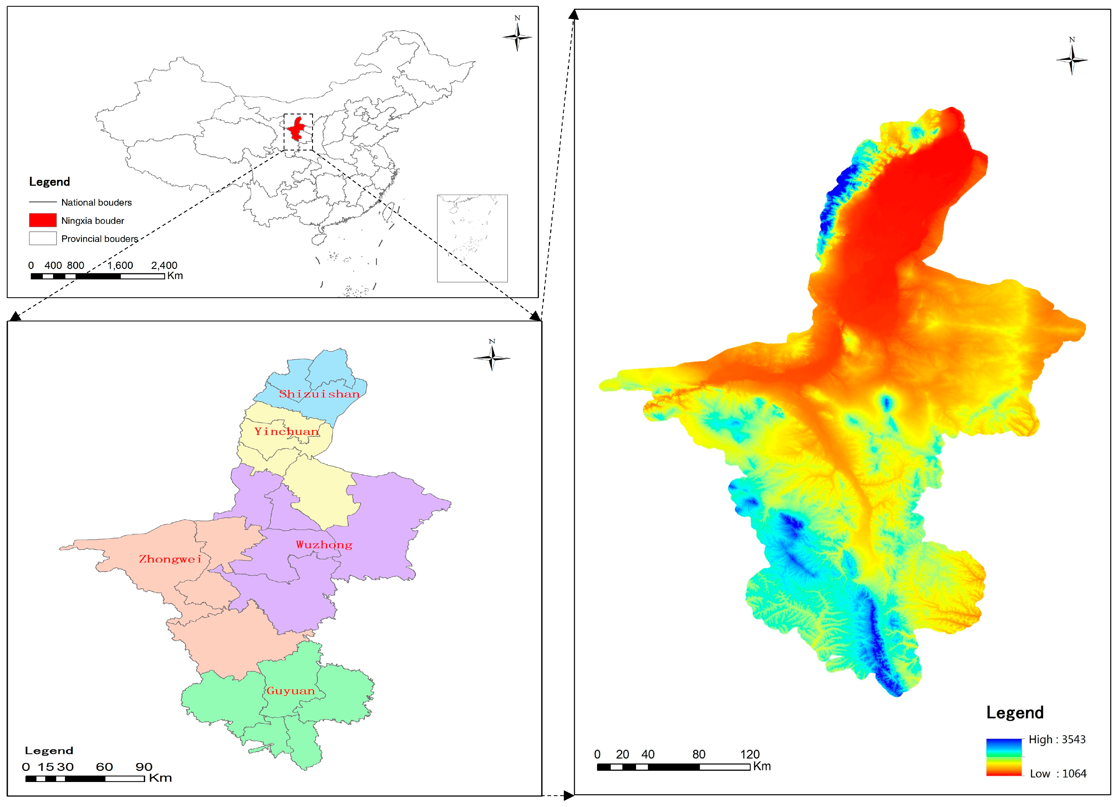
2.1. Study Area

The Ningxia Hui Autonomous Region represents one of the most significant administrative divisions in Northwest China (Figure 1). It is situated in the northwestern frontier area of the country, adjacent to the west bank of the middle reaches of the Yellow River [36]. The region’s geographic coordinate frame is situated between 35°14′ and 39°23′ north latitude and 104°17′ and 107°39′ east longitude. It shares its eastern border with Shaanxi Province, its western and northern borders with the Inner Mongolia Autonomous Region, and its southern border with Gansu Province. In terms of administrative divisions, Ningxia encompasses five prefectural-level cities, which are further subdivided into nine municipal districts, two county-level cities, and 11 counties. The total land area of Ningxia is approximately 51,900 km2. From a natural geographical perspective, Ningxia is situated in a transitional zone between the desert and the Loess Plateau, with diverse topography and geomorphology. The region’s topography is characterized by elevated terrain in the south and low-lying areas in the north, often in narrow bands from south to north. In terms of climate, Ningxia has a temperate continental climate characterized by four distinct seasons, sparse precipitation, and long hours of sunshine. The soil types in Ningxia are the result of complex interactions between natural and anthropogenic factors, such as terrain, geomorphology, vegetation, climate, and farming practices. These factors have shaped the region’s soil diversity, which is characterized by horizontal and vertical zonation. There is a notable correlation between soil types and vegetation in the area, as observed by Abd [37].
In addition, hydrological information, as a key environmental element, has a profound impact on the succession of land cover types and the transformation of land use patterns [38]. Ningxia Hui Autonomous Region has long been plagued by water scarcity, and the spatial distribution of water resources is extremely uneven. The main stream of the Yellow River and its tributaries, such as Qingshui River, Kushui River, Jing River, etc., constitute the main surface water system in Ningxia. The Yellow River stretches for 397 km in Ningxia, with gentle water flow. Thanks to this characteristic, the canals along the coast are crisscrossed, providing the main irrigation water source for local agricultural production. The total precipitation in Ningxia is scarce, with an average annual precipitation of only 289 mm. Correspondingly, the surface runoff scale in Ningxia is limited, with an average annual runoff of 9.493 × 10⁸ m3, an annual runoff depth of 18.3 mm, and a water production modulus of 1.83 × 10⁴ m3/km2. The overall water resources situation is not optimistic.

2.2. Data Sources and Processing

In this study, data from the Third China Land Survey are used as a reference, with the data from the First and Second Land Surveys subsequently normalized. This process primarily encompasses the standardization of land classification names and the geographic matching of point and line entities. The land use types are subsequently classified into six categories: farmland, forestland, grassland, construction land, water, and unused land. The data are subsequently transformed to the cell grid scale, with a spatial resolution of 30 m and a range of 9923 by 15,371. The standardized processed land use status data are presented in Figure 2. To gain insight into future patterns of land use change, socioeconomic, spatial, topographic, climatic, environmental, and spatial accessibility data are obtained to identify the drivers of land transformation. Furthermore, future land use is constrained by national spatial planning data. Consequently, data related to the ’three zones and three lines’ and other policy restrictions are integrated to simulate future land use change scenarios. Table 1 lists the sources of the data and the preprocessing steps used in this study, with all the data processed to the standard grid size.

3. Research Methods

3.1. Lines of Research and Methodology

As part of the ‘Territorial Spatial Planning’ of the Department of Land and Resources of the Ningxia Hui Autonomous Region, the specific framework of this study is shown in Figure 3.
(1)
Data collection and preprocessing: The initial step is to collect data pertaining to land use/cover, socioeconomic factors, and environmental conditions within the designated study area. This step is followed by necessary preprocessing, which includes data cleaning, format conversion, and spatial matching, to prepare the input data for the subsequent modeling tasks.
(2)
Optimization of the GMOP model: The second step is the optimization of land use through the utilization of the GMOP algorithm. This entails the definition of decision variables and the establishment of constraints and objective functions. Subsequently, solutions to the land use optimization problem under different control policy scenarios are obtained.
(3)
PLUS model parameterization and calibration: The essential parameters of the PLUS model are entered, such as those pertaining to land change drivers, land use conversion rules, neighborhood weights, and spatial constraints. It is essential to calibrate the PLUS model on the basis of historical data to guarantee that the model can accurately reflect the historical trend of land use change.
(4)
Uncertainty analysis: The IFS is employed to address the uncertainty inherent in the model.
(5)
Land change simulation analysis: The coupled model is run to simulate variations in the quantity and spatial distribution of land use under disparate control policy scenarios. The simulation results are analyzed to identify the prevailing trends and patterns of land use change.
(6)
Evaluation of the value of ecological services: The results of the land change simulation are combined to evaluate the ESV provided by different land use types and configurations. This process includes evaluations of provisioning, regulations, and cultural and support services.

3.2. PLUS-GMOP-Based Coupled Model

3.2.1. Modeling Principles

To comprehensively explore and simulate the evolutionary dynamics of land use under diverse control policies, an innovative coupled strategy, namely, the integration of the GMOP model with the PLUS model, is developed. The objective of this strategy is to leverage the distinctive capabilities of the two models to generate accurate and pragmatic land use change projections. The operational process of the coupled model can be divided into two principal stages:
(1)
Multiobjective optimization: In this phase, the GMOP model is employed to perform a multiobjective optimization task. By meticulously selecting decision variables, defining constraints, and establishing a set of objective functions, multiple objectives are comprehensively considered, including, but not limited to, the maximization of economic benefits derived from land use, the maximization of ecological value, and the coordination of economic and ecological development. GMOP employs sophisticated algorithms to identify optimal solutions across multiple objectives in parallel, resulting in the generation of a range of non-inferior solutions within the multiobjective space. These solutions represent the optimal trade-offs among the objectives under the given constraints, thereby providing a basic scheme for the subsequent spatialized simulation of land use change.
(2)
A simulation of land use change that incorporates spatial elements: The PLUS model is used to express the multiobjective optimization solutions output by the GMOP model in a spatial context. The PLUS model integrates the land expansion analysis strategy and a conditional meta-cellular automata model to transform the quantitative information from the optimal solutions into specific spatial layouts (Table 2). In this process, various land change drivers selected for this study, such as topography, traffic, and existing land use types, are considered. Moreover, parameters such as transformation rules and domain weights are applied. This approach ensures that the simulation results reflect not only the quantitative changes in land use but also a reasonable spatial distribution. It is worth mentioning that the PLUS software package (V1.2.5) provides convenience for this simulation, which is hosted on the Github platform (https://github.com/HPSCIL/Patch-generating_Land_Use_Simulation_Model).
It has a user-friendly interface that is easy for users to operate.

3.2.2. LSTM Model

Long short-term memory (LSTM) networks represent a distinctive variant of recurrent neural networks (RNNs). These methods have been developed with the objective of overcoming the challenges associated with gradient decay and gradient explosion that are inherent in traditional RNNs when dealing with long-term serial data [39,40]. In the context of forecasting the future land use demand, the PLUS model, despite integrating both linear regression and Markov chain models, is inherently constrained by vanishing and exploding gradient issues. Its information processing capacity is limited to a fixed time scale [30]. In light of the aforementioned challenges, the LSTM model is introduced in a deep learning architecture to accurately predict the area distribution and key input parameters of various land use types in 2030. This is achieved through the model’s excellent long-term dependency capture capability and flexible time scale adaptability, with the aim of facilitating efficient and accurate land resource planning and management.
The LSTM network is composed of a three-gate mechanism, comprising the forget gate, input gate, and output gate. The aforementioned gates regulate the flow of information in an adaptive manner, thereby facilitating the capture of long-term dependent information.
(1) Forget gate: The objective of the forget gate is to determine which information should be discarded or retained from the memory unit at each time step. This is achieved through the application of the following formula:
f t = δ ω f · s t 1 , x t + ρ f
In this context, δ represents the logical activation function, and ω f and ρ f denote the weight matrix and bias term of the forget gate, respectively. Additionally, s t 1 , x t signifies the hidden state of the previous time step and the input of the current time step.
(2) Input gate: The input gate is composed of two distinct components: a sigmoid layer, which determines which values will undergo modification, and a tanh layer, which generates a novel vector of potential values to be incorporated into the existing state. The formula for the input gate is as follows:
i t = δ ω i · s t 1 , x t + ρ i c t = tanh ω c · s t 1 , x t + ρ c
In this context, i t represents the output of the input gate and c t denotes the candidate memory cell state. Additionally, ω i and ω c are the correlation weight and bias, respectively, and ρ i and ρ c correspond to the same variables but for the input gate.
(3) Output gate: The output gate is responsible for determining which portion of the memory cell state is transmitted to the hidden state. This is accomplished through the application of the following formula:
o t = δ ω o · s t 1 , x t + ρ o s t = o t tanh c t
In this context, o t represents the output of the sigmoid function of the output gate, c t denotes the updated memory cell state, and s t signifies the final hidden state output.

3.2.3. Scenarios

The core challenge for achieving sustainable land use is to strike a balance between economic development and ecological protection [41,42]. To obtain a comprehensive and precise representation of the quantitative variations in land utilization and to conduct a comprehensive analysis of the evolving patterns of land use, four distinct land use scenarios were meticulously devised in this study. By employing the coupled GMOP-PLUS model to optimize the allocation of the land area, this study offers a scientifically and reasonably sound reference for decision-makers. The following four land use scenarios were established during this study:
(1) Business-as-usual (BAU) scenario: This scenario represents the baseline against which other scenarios are evaluated. This scenario depicts the natural evolution of land, considering any policy constraints and spatial control mechanisms. This scenario is established through the utilization of Markov chain projections, which are based on land use data from 2010 and 2020.
(2) Economic benefit priority (RED) scenario: The objective of this scenario is to identify the optimal means of maximizing the economic benefits associated with land use. The following formula is used to calculate the economic benefits of land:
f 1 x = m a x i = 1 6 x i d i
In this context, the symbol f 1 x represents the maximum economic output of land use and x i denotes the total area of the ith land use type. The variable i refers to the land use type, with values ranging from 1 to 6, representing agricultural land, forestland, grassland, building land, water, and unused land, respectively. Finally, the symbol d i denotes the economic output per unit area of the ith land use type. In conjunction with the Ningxia Statistical Yearbook, the economic benefits of farmland, forestland, grassland, and water were calculated on the basis of the output values of plantations and the forestry, animal husbandry, and fishery industries, respectively. The economic benefits of construction land were estimated from the GDPs of the second and third industries. The historical data were obtained from the Ningxia Statistical Yearbook (2010–2020) and uniformly normalized to a comparable price in 2010. The economic output values of farmland, woodland, grassland, construction land, and water were predicted to be 2.84, 0.04, 1.23, 149.92, and 3.10, respectively, in 2030 via the LSTM model (units: million yuan/ha).
(3) Ecological protection priority (ELP) scenario: The objective of this scenario is to optimize the ecological value of land use. The formula for calculating the ecological value of land is as follows:
f 2 x = m a x i = 1 6 x i e i
In this context, the symbol f 2 x represents the maximum ESV of land use, whereas the symbol e i denotes the ecological value of the ith land use type. The latter is expressed in million yuan per hectare and corresponds to values of 1.84, 6.54, 2.72, −1.32, 11.05, and 0.32 for agricultural land, forestland, grassland, construction land, watershed, and unutilized land, respectively.
(4) Economically and ecologically balanced (EEB) scenario: To achieve coordinated economic and ecological development and balance economic and ecological objectives, it is necessary to maximize the ecological and economic values of different land types:
m a x f 1 x , f 2 x

3.2.4. Restrictive Conditions

The RED, ELP, and EEB scenarios are also contingent upon historical land use patterns, planning controls, socioeconomic conditions, strategic objectives, and development projections.
(1) Total land area constraint: The total area of the study area is equal to the sum of the areas of all land use types:
i = 1 7 x i = 5,196,400   ha
(2) Total population constraint: It is imperative that the total population does not exceed the carrying capacity of land resources for human activities. On the basis of population and land statistics from 2010 to 2020, the total population of Ningxia in 2030 is projected to reach 8.19 million based on simulations with the LSTM model. Furthermore, the model indicates that the average population densities of agricultural land (farmland, forestland, and grassland) and construction land will be 0.42 and 16.38 persons per hectare, respectively.
0.42 × x 1 + x 2 + x 3 + 1.63 × x 4 8.19 × 10 6
(3) Food security constraints:
α 31 × f 0 × f 1 × 0.81 x 1 s × w × p
In this context, the variable α 31 represents the grain yield, with the lower limit corresponding to the current yield and the upper limit aligned with the target year yield. The term f 0 denotes the replanting index and f 1 refers to the ratio of grain species. The variable s signifies the per capita grain demand, which is projected to reach 517.3 kg/a by 2030. The term w represents the grain self-sufficiency rate. Given that Ningxia’s per capita arable land area is the second highest of any region in the country and because it is among the 12 major commercial grain production bases, the grain output should at least meet the requirements for regional self-sufficiency. Therefore, w is set to 100%. The size of the population in the prediction year is also considered. The LSTM model is used to predict f 0 , f 1 , and α 31 on the basis of historical data. The results are as follows: f 0 = 0.97, f 1 = 0.49, and α 31 ( 5603.68 ,   6931.77 ) . On the basis of the available data regarding land use in recent years, the area of arable land represents approximately 81% of the total farmland area after support facilities, such as ditches, roads, and field canopies, are removed.
(4) Constraints on the extent of farmland: The National Territorial Spatial Planning (2021–2035) strategy established a target for the protection of arable land in Ningxia at 1,169,220 hectares. According to the ‘Guidelines for the Evaluation of Resources and Environmental Carrying Capacities and Suitability for Territorial Spatial Development (for Trial Implementation)’, the upper limit of the carrying capacity of arable land in Ningxia is 1,463,310 hectares, given the relevant land and water resource constraints:
1,169,220   h a 0.81 x 1 1,406,310   h a
(5) Constraints on the area of forestland: The forestland area in Ningxia has continued to expand, with the forest coverage rate increasing from 11.9% in 2012 to 15.8% in 2020. In accordance with the ‘14th Five-Year Plan’ (2021–2025) for the protection and utilization of natural resources in Ningxia, land greening initiatives and ecological restoration projects have been promoted, with the objective of establishing Ningxia as a pivotal ecological security barrier in the northwestern region of the country. Furthermore, the forest coverage is projected to increase further in the future. The projected growth rate is significantly higher than that in the BAU scenario, with an anticipated increase from 8% to 20% by 2025. Consequently, the lower limit of the forest area in the target year is set at the same level as the forest area in the BAU scenario:
1,080,925   h a x 2
(6) Restrictions on the extent of construction land: Construction land encompasses urban construction land, village construction land, and other construction land. In accordance with the ‘Ningxia Territorial Spatial Planning (2021–2035)’ strategy, the newly designated urban construction land in 2035 should not exceed 0.3 times the current urban construction land scale. Consequently, the urban construction land area in 2030 should not exceed 1.2 times the current situation. The land designated for village construction remains unaltered, whereas the remaining construction land is calculated according to the average growth rate observed between 2010 and 2020. The lower limit value is defined as the construction land area in 2020:
350,487   h a x 4 398,390   h a
(7) Constraints on the grassland area: The grassland area in Ningxia has exhibited a persistent decline, from 2.51 million hectares in 2000 to 2.02 million hectares in 2020. This trend is projected to persist, with an anticipated decline to 1.77 million hectares by 2030. Consequently, the upper limit of the grassland area is defined as the current grassland area, whereas the lower limit is set based on a 10% decrease in the BAU scenario:
1,549,577   h a x 3 2,024,176   h a
(8) Constraints on the water area: Water surfaces and wetlands are of significant ecological importance. In recent years, the Ningxia region has implemented measures to enhance wetland protection, including the restoration of farmland to its natural state and the implementation of ecological protection and restoration initiatives. Ningxia’s water resources are sourced from the Yellow River in the majority of cases, with an estimated 90% of the region’s water originating from this source. In accordance with the strategies of ecological protection and high-quality development in the Yellow River Basin, the total volume and efficiency of water use in Ningxia have been subjected to rigorous control. As a consequence of the combined effects of enhanced protection and strict control, the watershed area of Ningxia has remained stable over time. Accordingly, the minimum and maximum watershed areas from 2000 to 2020 are employed as constraints for the watershed area in 2030:
96,700   h a x 6 110,011   h a
(9) Constraints on the area of unused land: Due to the limited availability of land resources and under the dual pressures of strict land use control measures and economic development, unused land can only be reclaimed and occupied in significant quantities to satisfy development needs. A substantial amount of unused land is expected to be converted to grassland and farmland in Ningxia from 2000 to 2020. Furthermore, the declining trend of unused land is projected to persist in 2030. It follows that the upper limit of the area of unused land is the current area of unused land, whereas the lower limit is the area of unused land in the BAU scenario:
165,791   h a x 7 249,720   h a
(10) The decision variables are constrained to be nonnegative:
x i 0 , i = 1 ,   2 ,   3 ,   4 ,   5 ,   6
The designation of permanent basic farmland as a land use constraint is crucial for ensuring food security. The implementation of control measures, such as the relocation of industrial projects to parks and the centralization of town development and construction areas, has transformed the corresponding areas into the primary focus for future construction. Consequently, these regions have been designated priority development areas for construction land.

3.2.5. Driving Force

In-depth studies of the driving factors of land use change and the associated socioeconomic and ecological environmental effects are of tremendous theoretical importance in revealing the intrinsic mechanism of the expansion of land use types and the probability of the transfer of land classes [43,44]. The results of these studies aid in understanding the potential drivers of land use change and provide a solid theoretical basis for predicting the future spatial distribution of land use.
Land use change is an extremely complex process that is influenced by numerous factors. In general, the three main forces driving land use change are natural conditions, socioeconomic factors, and development feasibility considerations, such as policies and regulations [9,30,31]. In this study, we referenced the preliminary requirements and suggestions of land use planning and spatial planning. Through a systematic review of the relevant literature and by considering the specific conditions of the research area, we selected 16 driving factors on the basis of principles such as data availability, consistency, quantifiability, and spatial heterogeneity (Figure 4). Specifically, we considered terrain factors (such as altitude, slope, and aspect), climate and environmental factors (such as annual average precipitation, annual average ground temperature, annual average evaporation, and soil type), distance factors (such as the shortest distance to towns, industrial parks, rivers, and roads), and socioeconomic factors (such as population density, per capita GDP, and nighttime light intensity).

3.3. Logistic Regression Analysis

To better understand and accurately describe the drivers of land use change, a binary logistic regression model is used for quantitative analysis. The model is suitable for explaining and predicting land use change in cases with dichotomous characteristics and is expressed as follows:
p = e β 0 + β 1 x 1 + β 2 x 2 + + β n x n 1 + e β 0 + β 1 x 1 + β 2 x 2 + + β n x n
Logistic functions are covariate nonlinear functions, and to find the regression coefficients, the ratio of the probability of an event occurring to the probability of it not occurring, called the odds, is first determined; then, the odds are logarithmically transformed to obtain the linear pattern of the logistic regression model:
l n p 1 p = β 0 + β 1 x 1 + β 2 x 2 + + β n x n
where x 1 , x 2 . . . x n are drivers of land use change and β 0 , β 1 . . . β n are the regression coefficients to be determined. In this work, the regression coefficient β, the statistic Wald χ2, the estimated significance level P, and the occurrence ratio OR are calculated via SPSS 22. Here, β indicates the change in cultivated land associated with a unit change in the corresponding driving factor, and the degree of change can be measured via OR. When β > 0 and is statistically significant (p < 0.05 at the 95% confidence level), OR increases with the selected factor if other factors remain unchanged; conversely, OR decreases with this factor. Waldχ2 indicates the degree of contribution of the driving factors to land use change and a large value represents a high degree of contribution.

3.4. ESV Calculation

The term ESV encompasses the full range of benefits that humans derive from ecosystems. These include services such as food production, water conservation, climate regulation, and biodiversity conservation [45]. ESV has become one of the key indicators of ecosystem quality and sustainability [46]. In this study, ESV was calculated via a modified equivalence coefficient, which can be used to assess spatial and temporal changes in ESV at large scales and for a variety of ecosystem services. Owing to the difficulty of obtaining land survey data, the lack of historical data, and the inconsistency of data standards, most existing studies use remote sensing image interpretation to obtain land use data for ESV calculations. However, the accuracy of remote sensing data cannot be verified and cannot meet the needs of actual land management; therefore, the land use data in this paper are based on China Land Survey data.
On the basis of the ESV measurement model proposed by Costanza [47] and Xie [48], ecosystem services were classified into nine categories, including gas regulation, water conservation, soil formation and protection, waste treatment, recreation and culture, etc., and the following revisions were made to the ESV equivalent factor table for Chinese ecosystems developed by Xie Gao Di on the basis of the actual situation in Ningxia. First, unused land is dominated by bare and sandy land and is therefore equivalent to desert. Second, the water area is the area-weighted average of water systems and wetlands. Third, the negative impacts of construction land on the ecosystem in terms of water resource conservation and waste treatment are estimated as services via the alternative cost method, where water resource conservation is approximated by the average annual value of water used for domestic and industrial/commercial purposes and waste treatment is estimated based on the value of social labor required to treat different types of waste. The revised ESV equivalent factor for terrestrial ecosystems in Ningxia is shown in Figure 5a.
The ESV in each network was calculated in the following way:
E S V i = D × a × j = 1 9 E i j
In Equation (19), E S V i is the ESV of a grid encompassing land use type I and D is the standard ESV equivalent, which is equal to 1/7 of the market value of grain production per hectare. Notably, D is calculated from the production and area of major grain crops (corn, wheat, rice, and soybean) in Ningxia from 2010 to 2020 as RMB 2327.5 per hectare per year. Moreover, in the equation, a is the area of each grid, equal to 0.9 hectares, and E i j is the value equivalent of the j-th ecosystem service function in a grid with land use type i. Through the above calculation, the ESV per unit area of different terrestrial ecosystems in Ningxia can be determined, as shown in Figure 5b.

4. Simulation and Analysis of Land Use Change

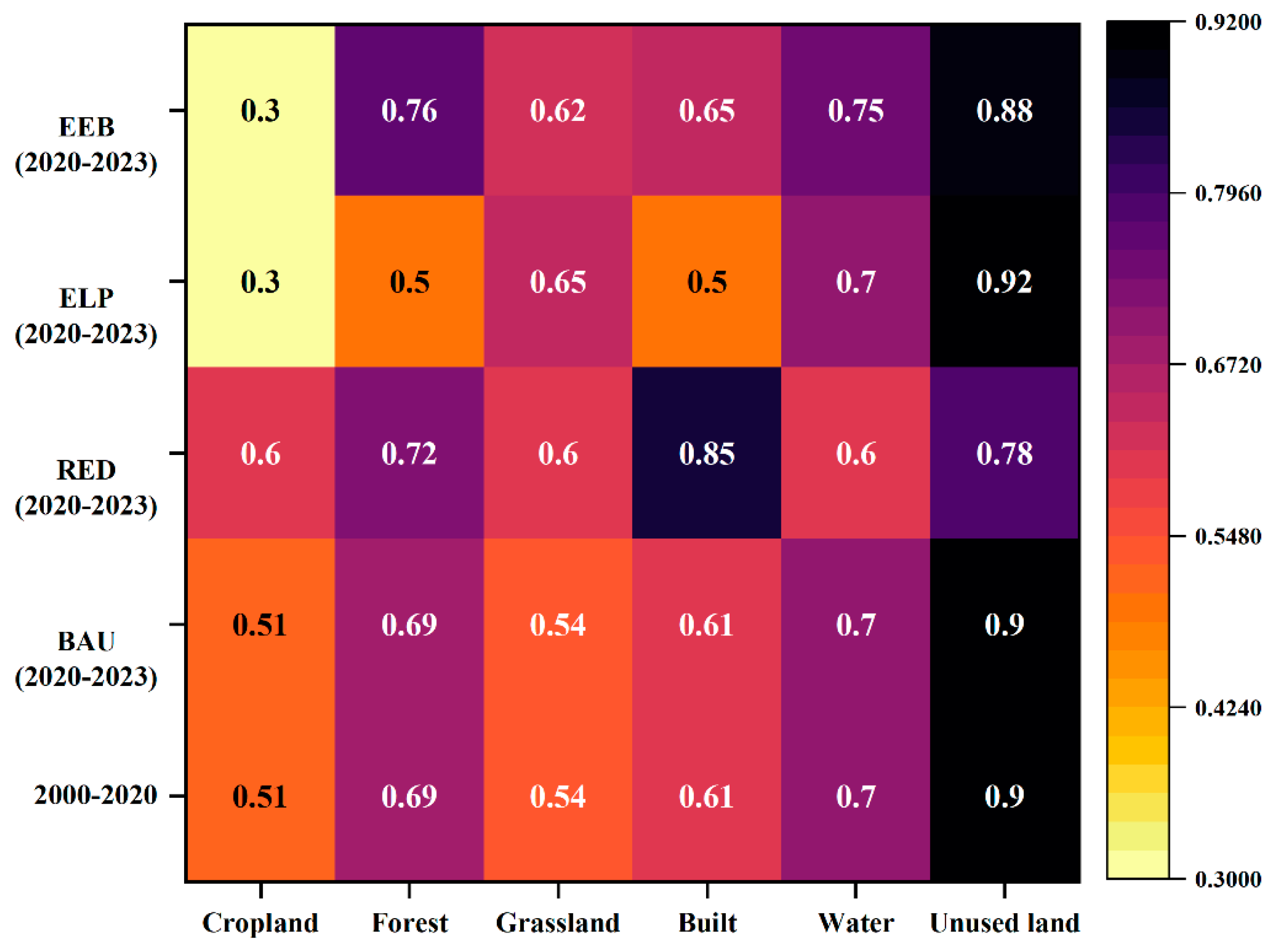
4.1. Accuracy Verification

On the basis of the spatial land use patterns in 2010, the simulated land use situation is compared with the actual land use situation in 2020 and the simulation error of the PLUS model is calculated through cross-validation. To comprehensively evaluate the prediction accuracy of the PLUS model, the kappa coefficient, FOM coefficient, and accuracy based on the number of predicted grids are used as evaluation indicators in this study. The comprehensive analysis of these indicators provides a scientific basis for assessing the performance of the PLUS model in predicting land use change. The kappa coefficient of the simulated spatial pattern of land use in 2020 is calculated to be 0.819 and the FOM coefficient is 0.31, indicating that the PLUS model yields good simulation accuracy and accurately reflects the changes in the spatial pattern of land use.

4.2. Land Use Change

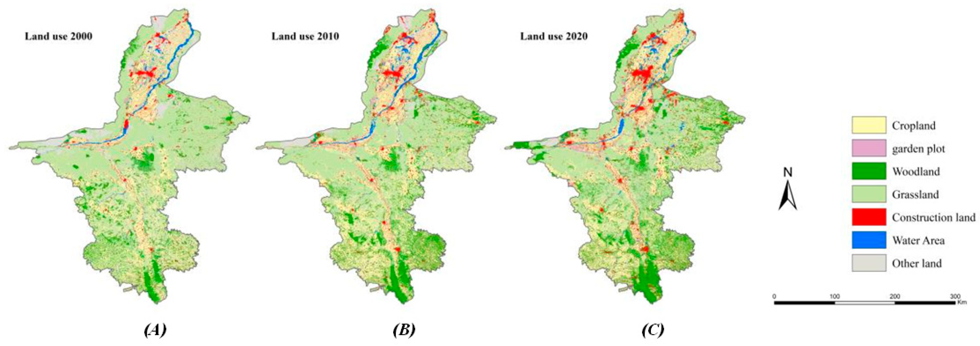
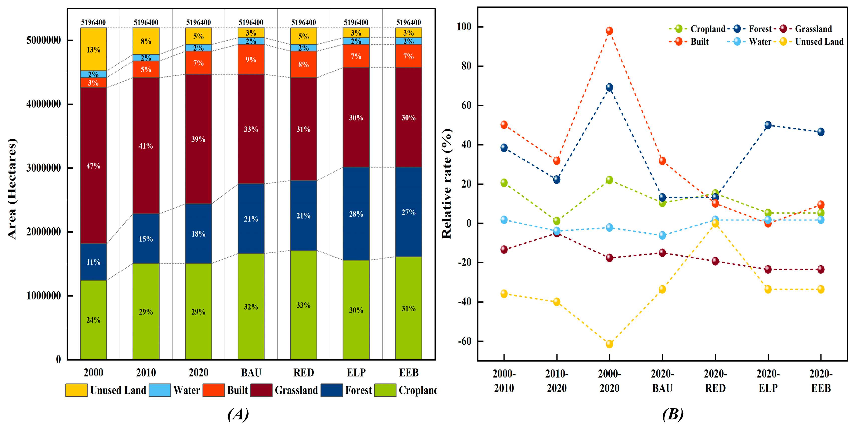
4.2.1. Analysis of Land Use Change

To accurately capture the spatial changes in land use in 2030, the above coupled model is used to spatially express the changes in the quantity of land use by adopting different parameters, driving factors, land use conversion rules, domain weights, spatial constraints, etc. Figure 6A shows the changes in the quantity and spatial distribution of land use from 2020 to 2030 under different parameter settings.
Influenced by external factors such as human activities and climate change, both the structure and distribution of land use in Ningxia have undergone significant changes. From 2000 to 2010, the area of grassland decreased by 3.2 × 10⁵ ha, as the land category with the greatest area change, and the rate of decrease in the area of grassland decreased with increasing attention given to environmental protection from 2010 to 2020. From 2000 to 2020, with the process of urbanization, the area of construction land increased from 170,000 ha to 3.505 × 10⁵ ha, with construction land mainly replacing arable land (43.95%), grassland (34.99%), and unused land (11.74%). Similarly, there was a large increase in the area of forestland, which increased by 69.2% over the 20-year study period, from 564,600 ha in 2000 to 955,500 ha in 2020; overall, 60.73% of the new area originated from grassland, and 24.09% originated from returning farmland to forests. The area of unused land decreased by 61.5%, from 6.489 × 10⁵ ha to 249,800 ha, with transformations mainly to grassland (55.53%), arable land (20.03%), and land used for construction (17.21%). The area of water basically remained unchanged. Notably, the degree of land change from 2000–2010 was greater than that from 2010–2020. For example, in 2010, the areas of cropland, forestland, grassland, and construction land increased by 20.6%, 38.5%, −13.4%, and 50.2%, respectively, compared with the levels in 2000; in 2020, the cropland, forestland, grassland, and construction land areas increased by 1.2%, 22.2%, −5%, and 31.8%, respectively, compared with those in 2010.
The land use structure and distribution in Ningxia changed significantly during 2000–2020 due to external factors such as human activities and climate change, and this example provides a reference for a realistic scenario for our study. From the perspective of changes in land use types, the decrease in grassland area and the increase in construction land and forestland in Ningxia are consistent with the conclusion found in our study that the expansion of construction land leads to ESV loss and the expansion of forest promotes ESV growth. This indicates that our proposed PLUS-GMOP coupled model has practical application value for analyzing such land use changes and their impacts on ESVs. For example, the substantial increase in forest area in Ningxia, mainly due to grassland and farmland returning to forest, may have led to significant changes in the value of ecosystem services. If our coupled model is used for evaluation, it is expected to quantify this more accurately and provide a scientific basis for local ecological protection and land use decisions.

4.2.2. Analysis of the Forces Driving Land Use Change

Table 3 shows that the driving factors of arable land changes along the Yellow River Ecological and Economic Belt in Ningxia are elevation, distance to the nearest city, and changes in population density. In general, natural endowment is the basic constraint on the increase in arable land. In areas with low elevation, low slope, and good irrigation conditions, the loss of soil, water, and nutrients is low, the cost of reclaiming arable land is low, and the land is suitable for agriculture; therefore, the probability of arable land use change occurring is high. If close to cities and roads, uncultivated land is preferentially converted to building land for the rapid realization of income due to the high accessibility and high potential for economic gain of the land. Moreover, these areas have few reserve resources that can be reclaimed via conversion to arable land and can be exploited only in certain areas far from cities and roads. In addition, changes in population density are positively related to increases in arable land. Notably, many ecological migrants have moved from the mountainous areas of southern Ningxia to places such as Xingqing District and Yongning County along the Yellow River Ecological and Economic Belt. Foreign migrants relocate to the countryside to engage in agricultural production and to meet various production and living requirements, and they perform land development, thus increasing the area of arable land. Second, the influx of a foreign population into a city promotes urban development, and the operation of a city consumes large amounts of resources; thus, the increased demand for agricultural products indirectly increases the amount of arable land needed for production.

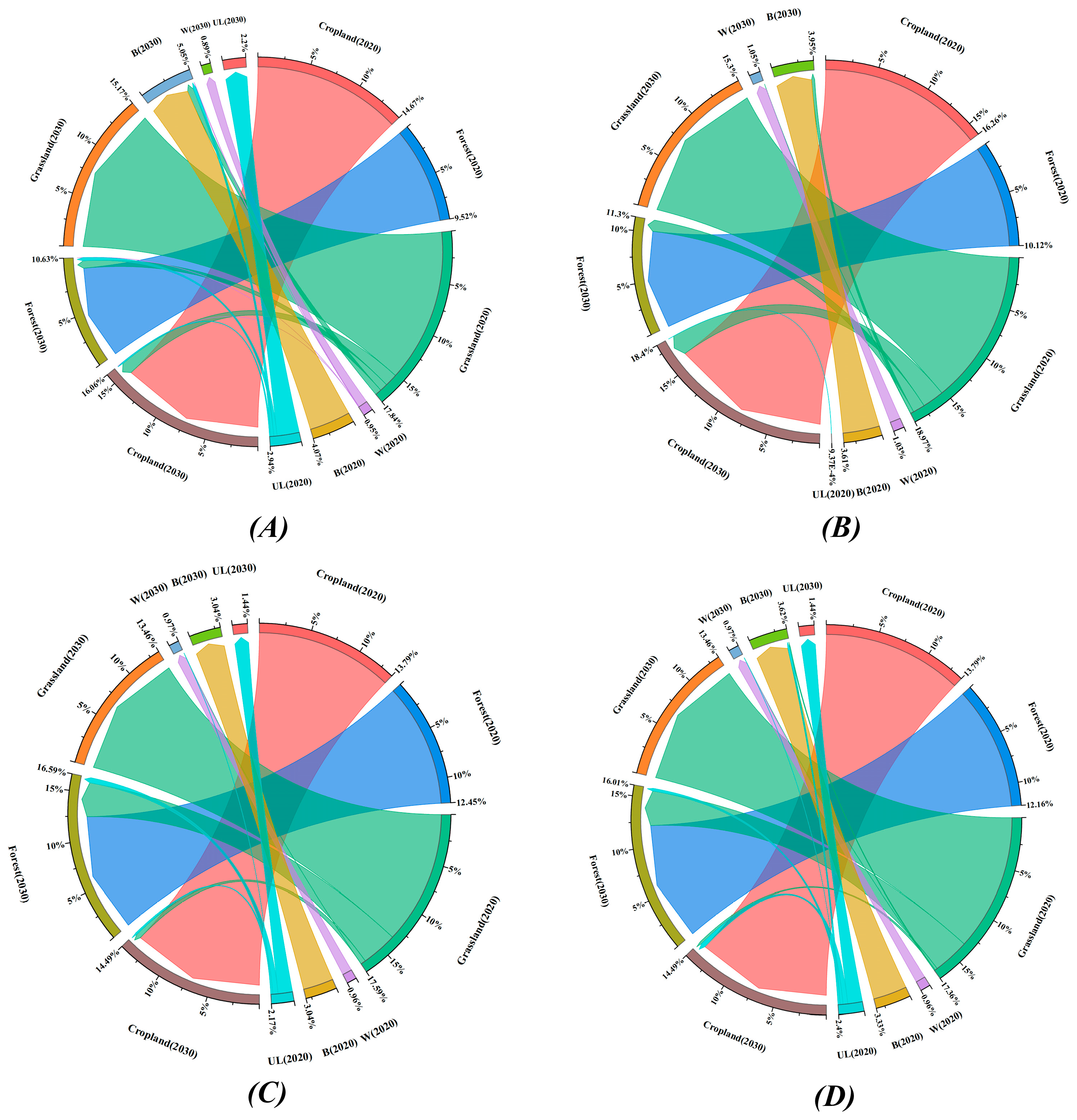
4.3. Multiscene Land Transformation Analysis

The elasticity coefficient of land use transformation reflects the ease of transformation of a certain type of land use to another type, which can be defined by the model parameter ELAS (Efficient Largescale Stereo-matching; ranging from 0 to 1). The ELAS parameter refers to the probability of expansion or contraction of a land use type, which reflects the dynamics of a certain land use type during the simulation period [49]. If the ELAS value is high, the land use type is likely to expand and potentially change considerably in a selected future simulation period; conversely, a low ELAS value implies that the land use type is likely to decrease in area or remain unchanged. To accurately represent the dynamic process of land use conversion, the rate of land use change from 2000 to 2020 is used to determine the ELAS for the BAU scenario; then, the values for the other three scenarios are determined on the basis of the details of each scenario and information from other studies. The final conversion probability matrix is then obtained, as shown in Figure 7.
In the BAU scenario, the expansion rate of construction land displays a significant upward trend, as shown in Figure 6B, with a growth rate as high as 31.72%, which not only exceeds the level in 2020 but is also significantly higher than that in the EPS, at 10.10%, and in the EEB scenario, at 9.47%. In this scenario, the expansion of construction land mainly results from the conversion of grassland and unused land (Figure 8A). Specifically, the areas of grassland, unused land, and water decreased the most, with the most significant decrease in the area of grassland, amounting to 3.03 × 10⁵ ha, a reduction of 14.96%, which occurred before 2010. In contrast, the water area displayed the lowest reduction at 6.19%, corresponding to an area of 6.7 × 10³ ha. In this scenario, the shift in land use mainly involved transforming grassland and unused land into arable land, forestland, and land for construction.
In the RED scenario, significant increases in the areas of arable land, forestland, and construction land were observed. The specific data revealed that the expansion rates of arable land, forestland, and construction land reached 15.10%, 13.12%, and 11.6%, respectively. In contrast, the decrease in the total area of grassland and unused land was 19.13%. Figure 8B further shows that land use changes in the RED scenario tend to maximize economic benefits, with a decrease in ecological land, and the main feature of land type conversion is the transfer of grassland to cropland, forestland, and construction land. The specific area of transformation reached 3.9111 × 10⁶ ha.
In the ELP scenario, construction land has a serious negative impact on ESV, so the area of construction land remains basically unchanged in this scenario; the area of forested land displays a significant growth trend, increasing by 13.12% compared with the areas in the BAU and RED scenarios. This growth mainly comes from the use of grassland and unused land, totaling 4.77 × 10⁵ ha. Combined with Figure 8C, it can be further observed that the transfer of land use types in the ELP scenario is manifested mainly in the conversion of grassland to cropland and forestland.
In the EEB scenario, the forest area substantially increases. Specifically, the increase in forest area reaches 4.44 × 10⁵ ha, with a growth rate of 44.45%. This growth trend is also reflected in the expansion of construction land, which exhibits the second-highest growth rate at 9.47%. Additionally, the areas of grassland and uncultivated land clearly decrease. The decrease in the area of grassland is 4.75 × 10⁵ ha, and the decrease in the area of unused land reaches 8.4 × 10⁴ ha. Figure 8D illustrates the shifting characteristics of land use types in the EEB scenario. The main transformations are the conversions of grassland and unused land into cropland and forest. In addition, in the ELP and EEB scenarios, the importance of the environment is emphasized, and consequently, the ecological land area displays a positive growth trend.
From the comparison of different scenarios, we can see the powerful ability of the PLUS-GMOP coupled model in describing complex land use changes. The rapid expansion of construction land in the BAU scenario and the significant growth of cultivated land, forestland, and construction land in the RED scenario reflect the differences in land use under different development orientations. Through multi-scenario simulation, the model can clearly present the dynamic changes of land use types under the influence of different factors.
In the RED scenario, land use changes tend to maximize economic benefits, which is consistent with the consideration of the impact of socioeconomic factors on land use in the model. Through the model, we can further explore the long-term impact of this economically oriented land use change on the value of ecosystem services and provide a quantitative basis for balancing economic development and ecological protection. The ELP and EEB scenarios place a strong emphasis on environmental protection, and the model accurately captures the significant increase in forest area and control of construction land under this orientation. This indicates that the model has high accuracy in simulating policy-guided land use changes. Future research can use this model to deeply analyze the effects of enhancing the value of ecosystem services and the optimization path of land use structure under different environmental protection policy intensities. At the same time, the transformation of grassland and unused land in each scenario provides rich real-life cases for the parameter optimization of the model. Through the analysis of these cases, the parameter settings of the transformation of different land use types in the model are further improved, and the simulation accuracy and prediction ability of the model for land use changes in different regions and different development scenarios are improved so that it can better serve the land use, scientific management, and sustainable planning of resources.

4.4. Changes in the Value of Ecological Services

In this study, the method of equivalent coefficients is combined with a land use transfer matrix (as shown in Figure 7) to establish the transfer matrix of ESV in the study area between 2000 and 2030. This is done to explore the effect of the change in the quantity of land use on the ESV. According to the analysis, the total ESV continues to increase under the different development scenarios. All individual ESVs display growth, except for water protection and waste services in the BAU scenario and waste treatment and soil formation and protection services in the RED scenario. Notably, the most significant growth in total ESV is in the ELP scenario, whereas in the BAU and RED scenarios, the growth rates are relatively low at 0.28% and 1.03%, respectively; these values are much lower than the growth rate of 12.91% in the ELP scenario and 11.21% in the EEB scenario.
The analysis results indicate that the increase in forestland is the main factor leading to the increase in the ecological service value. Specifically, between 2000 and 2020, the increase in forest area led to an increase in ESV of $28.937 billion, contributing 64.24% to the total increase in ESV. This contribution displays a further upward trend in the 2030 projections, increasing to 79.63%, 93.83%, 93.43%, and 92.57% of the contribution of the forest area to the increase in ESV in the BAU, RED, ELP, and EEB scenarios, respectively.
Moreover, the establishment of construction land and newly cultivated land in the process of urbanization was identified as the main land use trend resulting in the loss of ESV. Between 2000 and 2020, the ESV decreased by 9.207 billion yuan due to the increase in the area of construction land, accounting for 30.56% of the total decrease in ESV, which occurred mainly from 2000–2013. Then, the rate of loss of ESV due to construction land occupation gradually decreased after 2014. Specifically, in the different scenarios, the ESV loss due to construction expansion in the BAU, RED, and EEB scenarios was 3.485 billion yuan, 1.514 billion yuan, and 1.658 billion yuan, respectively, accounting for 41.72%, 24.96%, and 34.05% of the total loss of ESV in each scenario. Moreover, under the influence of arable land protection policies, a large amount of land was converted to arable land, which led to significant ESV losses. From 2000 to 2020, in the BAU, RED, ELP, and EEB scenarios, the ESV losses due to land being reclaimed for cropland were $11.854 billion, $2.985 billion, $3.715 billion, $762 million, and $758 million, respectively. However, overall, the increase in ESV was greater than the decrease in ESV, indicating that the ecological environment as a whole is improving, as the country is focusing more on protecting the environment.
The PLUS-GMOP coupling model provides strong support for the work of establishing the ESV transfer matrix through the equivalent coefficient method and the land use transfer matrix in this study. The land use changes accurately simulated by the model provide a basic data guarantee for determining the impact of changes in the area of different land use types on ESV. For example, the trend of forest area increase simulated by the model is consistent with the conclusion in the study that the increase in forest area is the main factor in the increase of ESV, which strongly verifies the reliability of the model in reflecting the relationship between the ecosystem and land use.
The model also played an important role in the conclusion that construction land and newly cultivated land lead to ESV loss. The dynamic changes in land use presented by the model can intuitively show the spatiotemporal process of construction land expansion and cultivated land reclamation during urbanization, thus providing a basis for quantifying the negative impact of these two land use trends on ESV.

4.5. Discussion

In this study, we innovate the PLUS-GMOP coupled model to simulate and predict land use changes in the Ningxia Hui Autonomous Region. The coupled model is created by integrating the GMOP model with the PLUS model. The uncertainty parameters in the model are represented by intuitionistic fuzzy numbers. The accuracy of the model was verified using historical data from 2010 to 2020. Compared with the FLUS model, the model has higher simulation accuracy. Specifically, the kappa coefficient of the model is 0.819, indicating an increase of 12.19%. Furthermore, the FOM coefficient is 0.31, indicating an increase of 17.81%. The results show that the coupled model has good simulation accuracy and can accurately reflect changes in the spatial pattern of land use. This high-precision simulation capability mainly arises due to the advantages of model coupling: the GMOP model provides an optimal solution for land use changes through its multiobjective optimization capability, whereas the PLUS model converts these optimal solutions into specific land use spatial distributions through its excellent spatiotemporal dynamic simulation capability. On the basis of the above advantages, we assume that in different future scenarios, the use of the PLUS-GMOP coupled model created in this study for simulation will provide a more reliable and accurate basis for land use planning and decision-making and aid in the sustainable use of land resources and effective protection of the ecological environment.
In terms of driving force analysis, we quantitatively analyze the forces driving land use change in the Ningxia Hui Autonomous Region through a binary logistic regression model, revealing the significant influences of multiple factors, such as natural conditions, socioeconomic factors, and spatial accessibility, on land use change. The analysis results show that topographic factors (such as altitude and slope), population density, and distance from cities and transportation facilities are the key forces affecting land use change [30,31]. The joint action of these factors determines the direction and intensity of land use change. Notably, the forces driving land use change significantly differ in different scenarios. Under the RED scenario, land use change is driven mainly by economic interests, and the expansion of construction land and agricultural land is more significant; however, under the ELP scenario, the impact of policy orientation on land use change is more prominent, and the increase in forest area is the main effect. This difference in scenarios shows that the force driving land use change is not only affected by natural conditions and socioeconomic factors but also significantly regulated by policy orientation and management objectives [30].
We systematically analyze the impact of land use change on ESV through the PLUS-GMOP coupled model. The results reveal that there is a significant dynamic correlation between land use change and ESV. By simulating land use changes under different scenarios, we show that the impact of land use type conversion on ESV varies between scenarios and that the increase in forest area is a key factor driving the increase in ESV. From 2000 to 2020, the increase in forest area contributed greatly to the increase in ESV, and the level of this contribution continues to increase in the predictions made under various scenarios in 2030. This finding echoes the important position of forest ecosystems in many ecological studies [30,50,51]. Specifically, under the BAU scenario, the rapid expansion of construction land leads to a significant decline in the ESV, mainly due to the negative impact of construction land on ecosystem services, especially in terms of soil and water conservation and waste treatment. In the ELP scenario, the increase in forest area significantly increases the ESV, which shows that the value of regional ecosystem services can be effectively improved through reasonable land use planning and ecological protection policies. In addition, under the economic and ecological balance (EEB) scenario, a good growth trend of ESV is achieved by moderately controlling the expansion of construction land and increasing forest area, further confirming the importance of balancing economic development and ecological protection. On the basis of the above analysis, we believe that the impact of land use change on ESV can be optimized through reasonable policy regulation and planning. This model-based quantitative analysis provides a scientific basis for land use planning and ecological protection decision-making and aids in the sustainable use of land resources and effective protection of the ecological environment.

5. Conclusions

In this study, we focused on land use change and its impact on ecosystem service value (ESV), constructed a PLUS-GMOP coupled model, conducted in-depth analysis from multiple perspectives, and obtained the following important results:
(1) We constructed a coupled model of PLUS and GMOP for land use change analysis. This model successfully integrated the excellent spatiotemporal dynamic simulation capabilities of the PLUS model and the multiobjective optimization advantages of the GMOP model, effectively overcoming the limitations of applying a single model in land use research. The model addressed uncertain parameters through the intuitive fuzzy number (IFN) and utilized the LSTM model to predict future socioeconomic parameters, significantly improving the simulation accuracy and adaptability. In the case study of the Ningxia Hui Autonomous Region, the model accurately simulated the changes in land use types under different scenarios, clearly demonstrated the variations in land use structure and distribution under the influences of external factors, and fully verified the effectiveness and practicality of the model in complex geographical and socioeconomic environments.
(2) We conducted a driving force analysis based on the PLUS-GMOP coupled model. On the basis of the coupled model, we revealed that topographic factors (such as altitude and slope), population density, and distance to cities and transportation facilities were the key forces driving land use change. Natural conditions provided basic constraints for land use change, whereas socioeconomic factors drove the dynamic evolution of land use through policy guidance and economic benefits. Land use changes under different scenarios differed significantly, reflecting the important influences of factors such as economic development and ecological protection policies on land use patterns. These findings provided an important basis for understanding the internal mechanism of land use change and support for policymakers in scientific decision-making.
(3) We performed a multiscenario land use change simulation and ecological value analysis. We set four land use scenarios: business as usual (BAU), economic efficiency priority (RED), ecological protection priority (ELP), and economic and ecological coordinated development (EEB). The PLUS-GMOP coupled model was used to simulate and analyze land use changes under different scenarios. Then, the impact of land use change on the ecological value was further analyzed. The results revealed that there was a direct causal relationship between land use change and ESV. The increase in forest area was the key factor driving the increase in ESV, whereas the expansion of construction land and reclamation of cultivated land were the main causes of ESV loss. These results provided key empirical support for land use planning and ecological protection decision-making, highlighting the urgency and importance of balancing economic development and ecosystem protection in the land use planning process. Moreover, we emphasized the key role of accurately assessing ESV in land use decision-making and provided an important basis for rationally planning land use types, scales, and layouts on the basis of ecological value considerations.
We provided new research ideas and methods for land use change and ecosystem service value assessment. The research results offered important theoretical guidance and practical application value for the sustainable use of land resources and for ecological protection. In the future, it would be necessary to further study the weights of the factors driving land use change on the variation in ecological service value.

Author Contributions

Conceptualization, P.L. and W.K.; methodology, W.K. and L.W.; software, X.W., L.W. and Q.L.; validation, P.L. and X.W.; formal analysis, W.K. and L.W.; investigation, W.K. and L.W.; data Curation, W.K., L.W. and X.W.; writing-Original Draft, X.W. and W.K.; writing-Review and Editing, S.Y. and D.L.; visualization, X.Z., W.K. and X.W. All authors have read and agreed to the published version of the manuscript.

Funding

The Young Top Talent Project of Ningxia Hui Autonomous Region (no. RQ0039) and the Strategic Research and Consulting Project of the Chinese Academy of Engineering (no. 2023ZLZX0005).

Data Availability Statement

The data presented in this study are available upon request from the corresponding authors. The data are not publicly available due to the Regulations on State Secrets and the Specific Scope of Their Classification in Land Administration.

Acknowledgments

The authors would like to thank the editors and the anonymous reviewers for their crucial comments, which improved the quality of this paper.

Conflicts of Interest

Author Xinyi Wu was employed by the company Tibet Datang International Upper Nujiang River Hydropower Development Co, Ltd. The remaining authors declare that the research was conducted in the absence of any commercial or financial relationships that could be construed as a potential conflict of interest.

References

  1. Beillouin, D.; Cardinael, R.; Berre, D.; Boyer, A.; Corbeels, M.; Fallot, A.; Feder, F.; Demenois, J. A global overview of studies about land management, land-use change, and climate change effects on soil organic carbon. Glob. Change Biol. 2022, 28, 1690–1702. [Google Scholar]
  2. Assede, E.S.; Orou, H.; Biaou, S.S.; Geldenhuys, C.J.; Ahononga, F.C.; Chirwa, P.W. Understanding drivers of land use and land cover change in Africa: A review. Curr. Landsc. Ecol. Rep. 2023, 8, 62–72. [Google Scholar] [CrossRef]
  3. Yin, D.Y.; Li, X.S.; Li, G.I.; Zhang, J.; Yu, H.C. Spatio-temporal evolution of land use transition and its eco-environmental effects: A case study of the Yellow River basin, China. Land 2020, 9, 514. [Google Scholar] [CrossRef]
  4. Huang, J.L.; Tang, Z.; Liu, D.F.; He, J.H. Ecological response to urban development in a changing socio-economic and climate context: Policy implications for balancing regional development and habitat conservation. Land Use Policy 2020, 97, 104772. [Google Scholar] [CrossRef]
  5. Gasser, T.; Crepin, L.; Quilcaille, Y.; Houghton, R.A.; Ciais, P.; Obersteiner, M. Historical CO2 emissions from land use and land cover change and their uncertainty. Biogeosciences 2020, 17, 4075–4101. [Google Scholar]
  6. Davison, C.W.; Rahbek, C.; Morueta-Holme, N. Land-use change and biodiversity: Challenges for assembling evidence on the greatest threat to nature. Glob. Change Biol. 2021, 27, 5414–5429. [Google Scholar] [CrossRef]
  7. Wang, J.; Bretz, M.; Dewan, M.A.A.; Delavar, M.A. Machine learning in modelling land-use and land cover-change (LULCC): Current status, challenges and prospects. Sci. Total Environ. 2022, 822, 153559. [Google Scholar] [PubMed]
  8. Roy, P.S.; Ramachandran, R.M.; Paul, O.; Thakur, P.K.; Ravan, S.; Behera, M.D.; Sarangi, C.; Kanawade, V.P. Anthropogenic land use and land cover changes—A review on its environmental consequences and climate change. J. Indian Soc. Remote Sens. 2022, 50, 1615–1640. [Google Scholar]
  9. Briassoulis, H. Analysis of Land Use Change: Theoretical and Modeling Approaches; WVU Research Repository: Morgantown, WV, USA, 2020. [Google Scholar]
  10. Barbier, E.B. The policy implications of the Dasgupta review: Land use change and biodiversity: Invited paper for the special issue on “the economics of biodiversity: Building on the Dasgupta Review” in environmental and resource economics. Environ. Resour. Econ. 2022, 83, 911–935. [Google Scholar] [CrossRef]
  11. Patel, S.K.; Verma, P.; Shankar Singh, G. Agricultural growth and land use land cover change in peri-urban India. Environ. Monit. Assess. 2019, 191, 600. [Google Scholar] [CrossRef]
  12. Tobias, J.A.; Durant, S.M.; Pettorelli, N. Improving predictions of climate change–land use change interactions. Trends Ecol. Evol. 2021, 36, 29–38. [Google Scholar]
  13. Duveiller, G.; Caporaso, L.; Abad-Viñas, R.; Perugini, L.; Grassi, G.; Arneth, A.; Cescatti, A. Local biophysical effects of land use and land cover change: Towards an assessment tool for policy makers. Land Use Policy 2020, 91, 104382. [Google Scholar] [CrossRef]
  14. Tong, X.; Feng, Y. A review of assessment methods for cellular automata models of land-use change and urban growth. Int. J. Geogr. Inf. Sci. 2020, 34, 866–898. [Google Scholar] [CrossRef]
  15. Sasmito, S.D.; Sillanpää, M.; Hayes, M.A.; Bachri, S.; Saragi-Sasmito, M.F.; Sidik, F.; Hanggara, B.B.; Mofu, W.Y.; Rumbiak, V.I.; Hendri; et al. Mangrove blue carbon stocks and dynamics are controlled by hydrogeomorphic settings and land-use change. Glob. Change Biol. 2020, 26, 3028–3039. [Google Scholar] [CrossRef] [PubMed]
  16. Valle, D.; Izbicki, R.; Leite, R.V. Quantifying uncertainty in land-use land-cover classification using conformal statistics. Remote Sens. Environ. 2023, 295, 113682. [Google Scholar] [CrossRef]
  17. Gomes, E.; Inacio, M.; Bogdzevi, K.; Kalinauskas, M.; Karnauskait, D.; Pereira, P. Future land-use changes and its impacts on terrestrial ecosystem services: A review. Sci. Total Environ. 2021, 781, 146716. [Google Scholar] [CrossRef] [PubMed]
  18. Kannan, E.; Balamurugan, G.; Narayanan, S. Spatial economic analysis of agricultural land use changes: A case of peri-urban Bangalore, India. J. Asia Pac. Econ. 2021, 26, 34–50. [Google Scholar] [CrossRef]
  19. Chen, M.; Vernon, C.; Graham, N.; Hejazi, M.; Huang, M.; Cheng, Y.; Calvin, K. Global land use for 2015–2100 at 0.05 resolution under diverse socioeconomic and climate scenarios. Sci. Data 2020, 7, 320. [Google Scholar] [CrossRef]
  20. Ma, Y.; Wang, M.; Zhou, M.; Tu, J.; Ma, C.; Li, S. Multiple scenarios-based on a hybrid economy–environment–ecology model for land-use structural and spatial optimization under uncertainty: A case study in Wuhan, China. Stoch. Environ. Res. Risk Assess. 2022, 36, 2883–2906. [Google Scholar] [CrossRef]
  21. Sourn, T.; Pok, S.; Chou, P.; Nut, N.; Theng, D.; Hin, L. Assessing land use and land cover (LULC) change and factors affecting agricultural land: Case study in battambang province, Cambodia. Res. World Agric. Econ. 2023, 4, 41–54. [Google Scholar] [CrossRef]
  22. Ren, Y.; Lu, Y.; Comber, A.; Fu, B.; Harris, P.; Wu, L. Spatially explicit simulation of land use/land cover changes: Current coverage and future prospects. Earth-Sci. Rev. 2019, 190, 398–415. [Google Scholar] [CrossRef]
  23. Shen, X.; Wang, X.; Zhang, Z.; Lu, Z.; Lv, T. Evaluating the effectiveness of land use plans in containing urban expansion: An integrated view. Land Use Policy 2019, 80, 205–213. [Google Scholar] [CrossRef]
  24. Liang, X.; Guan, Q.; Clarke, K.C.; Liu, S.; Wang, B.; Yao, Y. Understanding the drivers of sustainable land expansion using a patch-generating land use simulation (PLUS) model: A case study in Wuhan, China. Comput. Environ. Urban Syst. 2021, 85, 101569. [Google Scholar] [CrossRef]
  25. Gong, J.; Du, H.; Sun, Y.; Zhan, Y. Simulation and prediction of land use in urban agglomerations based on the PLUS model: A case study of the Pearl River Delta, China. Front. Environ. Sci. 2023, 11, 1306187. [Google Scholar] [CrossRef]
  26. Liu, J.; Liu, B.; Wu, L.; Miao, H.; Liu, J.; Jiang, K.; Ding, H.; Gao, W.; Liu, T. Prediction of land use for the next 30 years using the PLUS model’s multi-scenario simulation in Guizhou Province, China. Sci. Rep. 2024, 14, 13143. [Google Scholar] [CrossRef]
  27. van Vliet, J.; Bregt, A.K.; Hagen-Zanker, A. Revisiting Kappa to account for change in the accuracy assessment of land-use change models. Ecol. Model. 2011, 222, 1367–1375. [Google Scholar] [CrossRef]
  28. Zhang, Z.; Hu, B.; Jiang, W.; Qiu, H. Spatial and temporal variation and prediction of ecological carrying capacity based on machine learning and PLUS model. Ecol. Indic. 2023, 154, 110611. [Google Scholar] [CrossRef]
  29. Zhao, X.; Wang, P.; Gao, S.; Yasir, M.; Islam, Q.U. Combining LSTM and PLUS models to predict future urban land use and land cover change: A case in Dongying City, China. Remote Sens. 2023, 15, 2370. [Google Scholar] [CrossRef]
  30. Xu, X.; Kong, W.; Wang, L.; Wang, T.; Luo, P.; Cui, J. A novel and dynamic land use/cover change research framework based on an improved PLUS model and a fuzzy multiobjective programming model. Ecol. Inform. 2024, 80, 102460. [Google Scholar] [CrossRef]
  31. Zhong, Y.; Zhang, X.; Yang, Y.; Xue, M. Optimization and simulation of mountain city land use based on MOP-PLUS model: A case study of Caijia Cluster, Chongqing. ISPRS Int. J. Geo-Inf. 2023, 12, 451. [Google Scholar] [CrossRef]
  32. Zhu, L.; Huang, Y. Multi-scenario simulation of ecosystem service value in Wuhan metropolitan area based on PLUS-GMOP model. Sustainability 2022, 14, 13604. [Google Scholar] [CrossRef]
  33. Ma, R.; Fan, Y.; Wu, H.; Zhu, L.; Ma, X.; Fan, X.; Zhang, H. Simulation of land-use patterns in arid areas coupled with GMOP and PLUS models. J. Agric. Resour. Environ. 2023, 40, 143. [Google Scholar]
  34. Fu, H.; Liang, Y.; Chen, J.; Zhu, L.; Fu, G. A New Framework of Land Use Simulation for Land Use Benefit Optimization Based on GMOP-PLUS Model—A Case Study of Haikou. Land 2024, 13, 1257. [Google Scholar] [CrossRef]
  35. Wang, Z.; Zhong, A.; Li, Q. Optimization of Land Use Structure Based on the Coupling of GMOP and PLUS Models: A Case Study of Lvliang City, China. Land 2024, 13, 1335. [Google Scholar] [CrossRef]
  36. Yan, Z.; Huixin, M.; Xiaoyu, Z.; Furong, Z.; Zhanjun, W.; Shuxing, F.; Sarah, O.S.; Pan, J.; Ma, Z.; Fan, J. Ningxia. In Climate Risk and Resilience in China; Routledge: London, UK, 2015; pp. 233–261. [Google Scholar]
  37. Abd El-Hamid, H.T.; Wei, C.Y.; Hafiz, M.A.; Mustafa, E.K. Effects of land use/land cover and climatic change on the ecosystem of North Ningxia, China. Arab. J. Geosci. 2020, 13, 1099. [Google Scholar] [CrossRef]
  38. Lopes, T.R.; Zolin, C.A.; Mingoti, R.; Vendrusculo, L.G.; de Almeida, F.T.; de Souza, A.P.; de Oliveira, R.F.; Paulino, J.; Uliana, E.M. Hydrological regime, water availability and land use/land cover change impact on the water balance in a large agriculture basin in the Southern Brazilian Amazon. J. South Am. Earth Sci. 2021, 108, 103224. [Google Scholar]
  39. Yu, Y.; Si, X.; Hu, C.; Zhang, J. A review of recurrent neural networks: LSTM cells and network architectures. Neural Comput. 2019, 31, 1235–1270. [Google Scholar] [CrossRef] [PubMed]
  40. Sherstinsky, A. Fundamentals of recurrent neural network (RNN) and long short-term memory (LSTM) network. Phys. D Nonlinear Phenom. 2020, 404, 132306. [Google Scholar] [CrossRef]
  41. Zhao, Y.; Hou, P.; Jiang, J.; Zhai, J.; Chen, Y.; Wang, Y.; Bai, J.; Zhang, B.; Xu, H. Coordination study on ecological and economic coupling of the Yellow River Basin. Int. J. Environ. Res. Public Health 2021, 18, 10664. [Google Scholar] [CrossRef]
  42. Zhang, Z.; Li, H.; Cao, Y. Research on the coordinated development of economic development and ecological environment of nine Provinces (regions) in the Yellow River Basin. Sustainability 2022, 14, 13102. [Google Scholar] [CrossRef]
  43. Ren, Y.; Lü, Y.; Fu, B.; Comber, A.; Li, T.; Hu, J. Driving factors of land change in China’s loess plateau: Quantification using geographically weighted regression and management implications. Remote Sens. 2020, 12, 453. [Google Scholar] [CrossRef]
  44. Liu, Y.; Wu, K.; Cao, H. Land-use change and its driving factors in Henan province from 1995 to 2015. Arab. J. Geosci. 2022, 15, 247. [Google Scholar] [CrossRef]
  45. Yang, J.; Xie, B.; Zhang, D. Spatial–temporal evolution of ESV and its response to land use change in the Yellow River Basin, China. Sci. Rep. 2022, 12, 13103. [Google Scholar] [CrossRef]
  46. Peng, H.; Hua, L.; Zhang, X.; Yuan, X.; Li, J. Evaluation of ESV change under urban expansion based on ecological sensitivity: A case study of three gorges reservoir area in China. Sustainability 2021, 13, 8490. [Google Scholar] [CrossRef]
  47. Costanza, R. Social goals and the valuation of ecosystem services. Ecosystems 2000, 3, 4–10. [Google Scholar] [CrossRef]
  48. Xie, G.; Zhang, C.; Zhen, L.; Zhang, L. Dynamic changes in the value of China’s ecosystem services. Ecosyst. Serv. 2017, 26, 146–154. [Google Scholar] [CrossRef]
  49. Jellal, R.A.; Lange, M.; Wassermann, B.; Schilling, A.; Zell, A. LS-ELAS: Line segment based efficient large scale stereo matching. In Proceedings of the 2017 IEEE International Conference on Robotics and Automation (ICRA), Singapore, 29 May–3 June 2017; IEEE: Piscataway, NJ, USA, 2017. [Google Scholar]
  50. Cui, F.; Wang, B.; Zhang, Q.; Tang, H.; De Maeyer, P.; Hamdi, R.; Dai, L. Climate change versus land-use change—What affects the ecosystem services more in the forest-steppe ecotone? Sci. Total Environ. 2021, 759, 143525. [Google Scholar] [CrossRef]
  51. Yu, Z.; Ciais, P.; Piao, S.L.; Houghton, R.A.; Lu, C.Q.; Tian, H.Q.; Agathokleous, E.; Kattel, G.R.; Sitch, S.; Goll, D.; et al. Forest expansion dominates China’s land carbon sink since 1980. Nat. Commun. 2022, 13, 5374. [Google Scholar] [CrossRef] [PubMed]
Figure 1. Location and digital elevation map (DEM) (original source from Information Center of Ningxia Department of Natural Resources) of the NingXia.
Land 14 00802 g001
Figure 2. Land use change map of Ningxia ((AC) are land use change maps of Ningxia in 2000, 2010, and 2020, respectively).
Land 14 00802 g002
Figure 3. Research roadmap (The numbers from 1 to 9 represent the order of calculation.).
Land 14 00802 g003
Figure 4. Schematic representation of the drivers of land change. (A) is DEM, (B) is the slope, (C) is the slope direction, and (D) is the soil type. (EG) denote the average annual precipitation, average annual ground temperature, and average annual evapotranspiration, respectively. (HL) denote the distance from settlements, distance from roads, distance from development zones, distance from the city, and distance from the river, respectively. (M) denotes the city lights at night, (N) denotes the GDP, (O) denotes the population density, and (P) denotes the spatial restrictions.
Land 14 00802 g004
Figure 5. ESV Calculation Matrix Diagram. (a) is a map of the ecosystem service value equivalent factors, (b) is the value of ecological services per unit area of land ecosystem, * denotes the absence of erosion, ** denotes the loss of value of three-waste pollution, *** denotes the consumption of freshwater resources, FP is food production, RW is raw materials, GR is gas regulation, CR is climate regulation, WC is water conservation, WD is waste disposal, SFC is soil formation and conservation, BC is biodiversity conservation, and EC is entertainment and culture. A, B, C, and D denote the supply services, regulating services, support services, and cultural services, respectively.
Land 14 00802 g005
Figure 6. Land use area change and rate of change chart. (A) represents the land use area change, and (B) represents the rate of area change.
Land 14 00802 g006
Figure 7. Schematic of the land use transfer probability matrix.
Land 14 00802 g007
Figure 8. Map of the land flow changes under four scenarios ((AD) represent BAU, RED, ELP, and EEB scenarios, respectively).
Land 14 00802 g008
Table 1. Data resource.
CategoryDataStatistical Object (Year)ResolutionData Resource
Land use datasetsTerritorial change survey (TCS)2010–2020Vector graphInformation Center of Ningxia Department of Natural Resources
Global 30-m land use cover map2000http://www.resdc.cn (accessed on 15 August 2024)
Socioeconomic statisticsPopulation and GDP2010–2020Non-spatial datahttps://tj.nx.gov.cn/ (accessed on 15 August 2024)
Food productionhttp://lswz.nx.gov.cn/ (accessed on 17 August 2024)
Area under cultivation
Food prices
Value of agriculture
Forestry
Socioeconomic spatial dataPopulation density20191 kmhttp://www.resdc.cn (accessed on 20 August 2024)
GDP20191 km
Light intensity2019400 m
Topographic dataSlope201930 mNASA ASTER Global Digital Elevation Model V003
Direction of slope201930 m
Elevation201930 m
Climate and environmental dataMean annual precipitation1960–20101 kmhttp://www.resdc.cn (accessed on 3 August 2024)
Mean annual ground temperature
Mean annual evaporation
Soil type
Spatial accessibilityDistance to rural settlements2019mmTCS
Distance to town30 m
Distance to the industrial parkmm
Distance from the Yellow River30 m
Distance to other roads30 m
Space-limited dataQuality farmland2022Vector graphhttp://www.resdc.cn (accessed on 27 August 2024)
Water-based wetland
Table 2. Parameters and description of the PLUS model.
ParametersImplication
dThe value of d is 0 or 1; a value of 1 indicates that there is a change from other land use types to land use type k and 0 indicates other conversions.
xA vector consisting of multiple drivers.
I(·)Indicator functions for decision tree sets.
hn(x)Prediction type for the nth decision tree for vector x.
MTotal number of decision trees.
P i , k d = 1 Probability of growth of land use type k in cell i.
D k t Impact of future demand on land use type k.
kAdaptive drive factor, depending on the gap between the current amount of land at iteration t and the target land use demand.
Ω i , k t Neighborhood effect of cell i, i.e., the proportion of land use components covered by k in the lower neighborhood.
c o n ( c i t 1 = k ) Last iteration.
n × n Total number of grid cells occupied by land use type k in the window.
wkThe weight between different land use types due to different neighborhood effects, for different land use types, has a default value of 1, but it can be defined by the model user.
G k t 1 , G k t 2 Difference between current quantity and future demand for land use type k in t − 1 and t − 2 iterations.
rRandom values from 0 to 1.
μ k Generating new land use patch thresholds for land use type k, as determined by the model user.
StepApproximate land use demand step size.
δ The decreasing threshold of the decay factor, which ranges from 0 to 1 and is set by the expert.
r1A normally distributed random value with a mean of 1 and a range from 0 to 2.
lDecay steps.
TMk,cA transition matrix which defines whether land is allowed to be converted to type c using type k.
Table 3. Logistic regression model correlation coefficient (DFU, DFR, and DFW represent the distance from cities and towns, distance from the main road, and distance from the water surface of the city river, respectively).
Implicit VariableDriving FactorRegression CoefficientStandard DeviationWald χ2
CroplandDFU0.520.03125.78
DFR−0.010.030.13
DFW0.010.050.01
Elevation−1.490.08335.45
Population0.490.0754.56
constant0.430.0460.79
ForestDFU0.640.02343.523
DFR1.190.04233.872
DFW0.350.0266.92
Elevation3.750.0265.476
Population−0.130.036.955
constant0.560.071517.868
BuiltDFU0.860.03215.23
DFR1.330.01262.173
DFW0.270.056.15
Elevation0.010.038.14
Population0.220.06137.232
constant0.580.05188.96
GrasslandDFU0.080.0115.194
DFR0.020.0113.606
DFW0.040.0542.135
Elevation0.10.03138.734
Population0.20.0522.366
constant0.620.05299.415
Disclaimer/Publisher’s Note: The statements, opinions and data contained in all publications are solely those of the individual author(s) and contributor(s) and not of MDPI and/or the editor(s). MDPI and/or the editor(s) disclaim responsibility for any injury to people or property resulting from any ideas, methods, instructions or products referred to in the content.

