
An Automatic Algorithm for Mapping Algal Blooms and Aquatic Vegetation Using Sentinel-1 SAR and Sentinel-2 MSI Data


 ,
,  ,
,
Abstract
1. Introduction
2. Materials
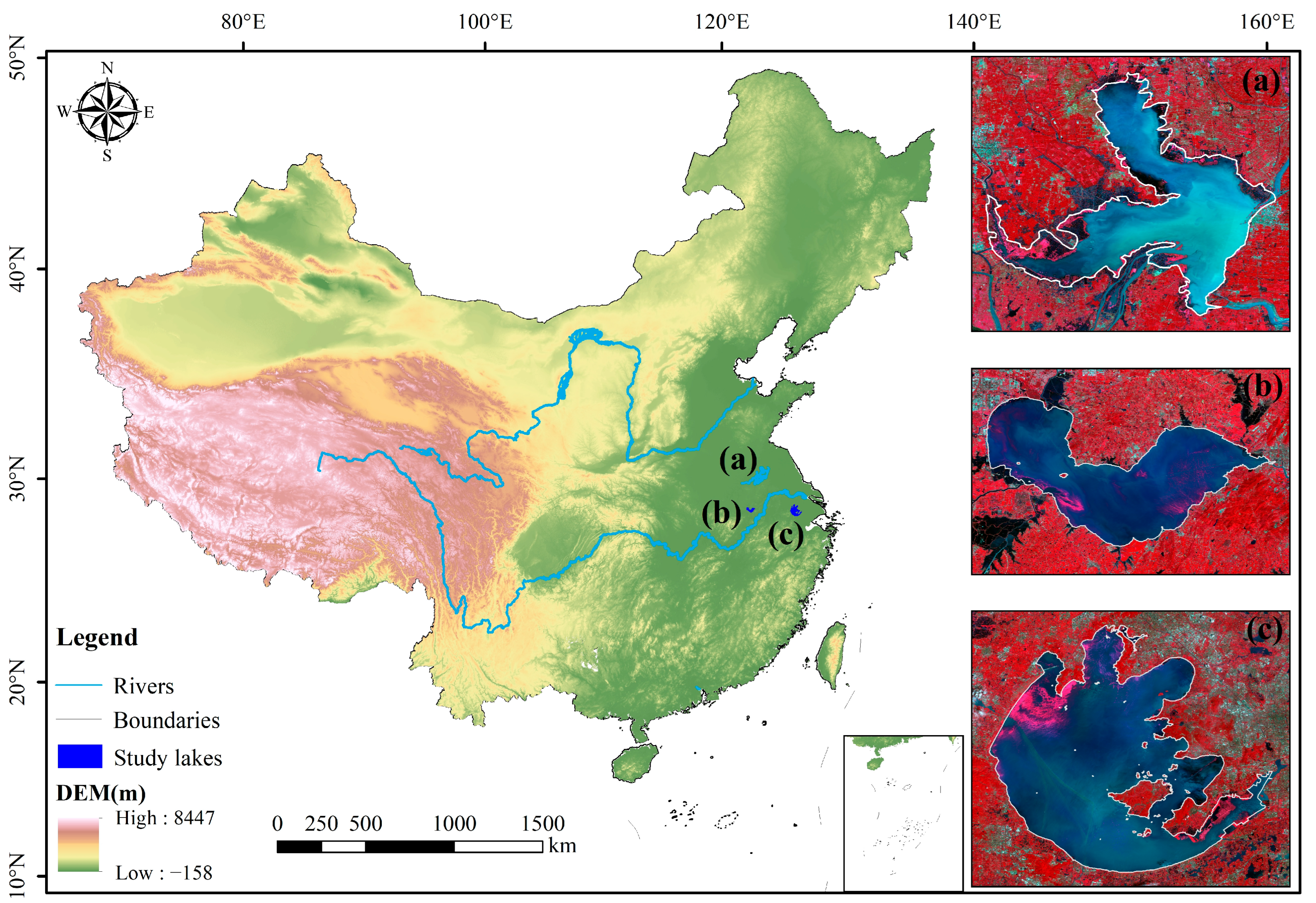
2.1. Study Area
2.2. Satellite Data
2.3. Field Data
3. Method
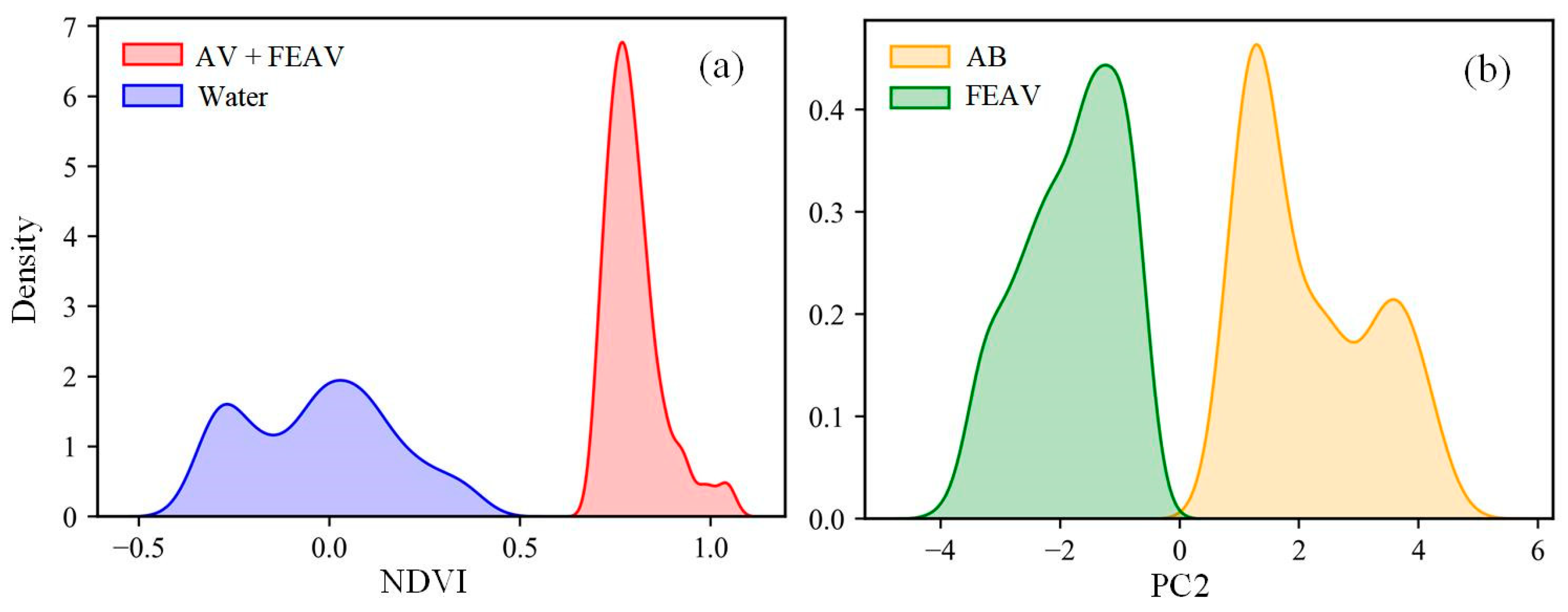
3.1. Mapping SAV
3.2. Mapping FEAV and AB
3.3. Assessment of Algorithm
- (1)
- Accuracy assessment based on field measured data. Confusion matrices were obtained between measured classes from field measured data and mapped classes derived from the algorithm proposed in this study, and overall accuracy (OA), Kappa, user accuracy (UA) and producer accuracy (PA) were calculated [36].
- (2)
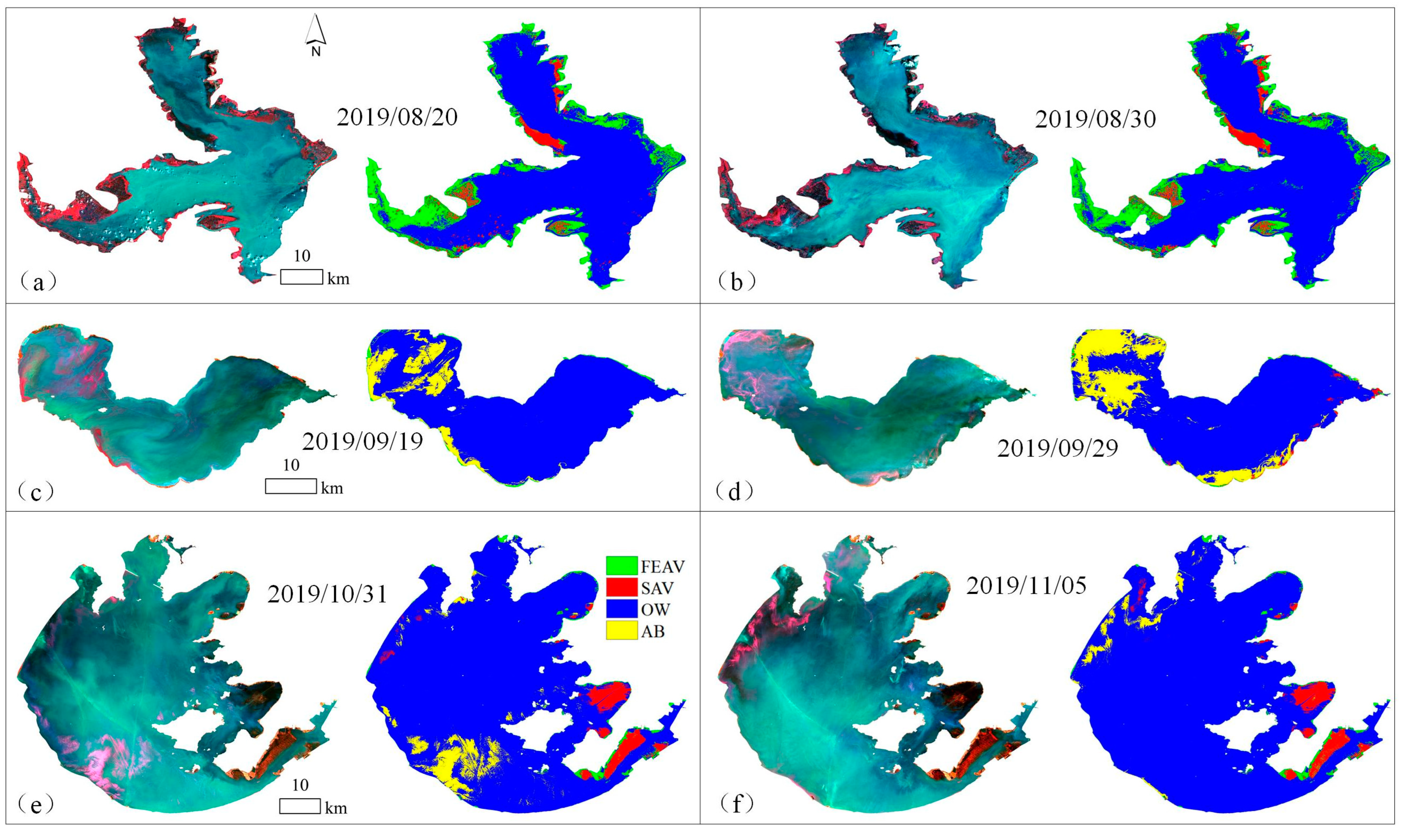
- Assessment by phenological features of aquatic vegetation. For lakes lacking FEAV and SAV samples, indirect validation was conducted by phenological feature of FEAV and SAV. Specifically, in a short timeframe, FEAV and SAV exhibit fixed spatial distribution and limited area change [37]. The similarity in spatial distribution of FEAV and SAV between adjacent temporally sequential images was assessed by Dice Coefficient [38] (Equation (8)).
4. Result
4.1. Validations of Algorithm
4.1.1. Validations by Field Measured Data
4.1.2. Assessment by Phenological Feature
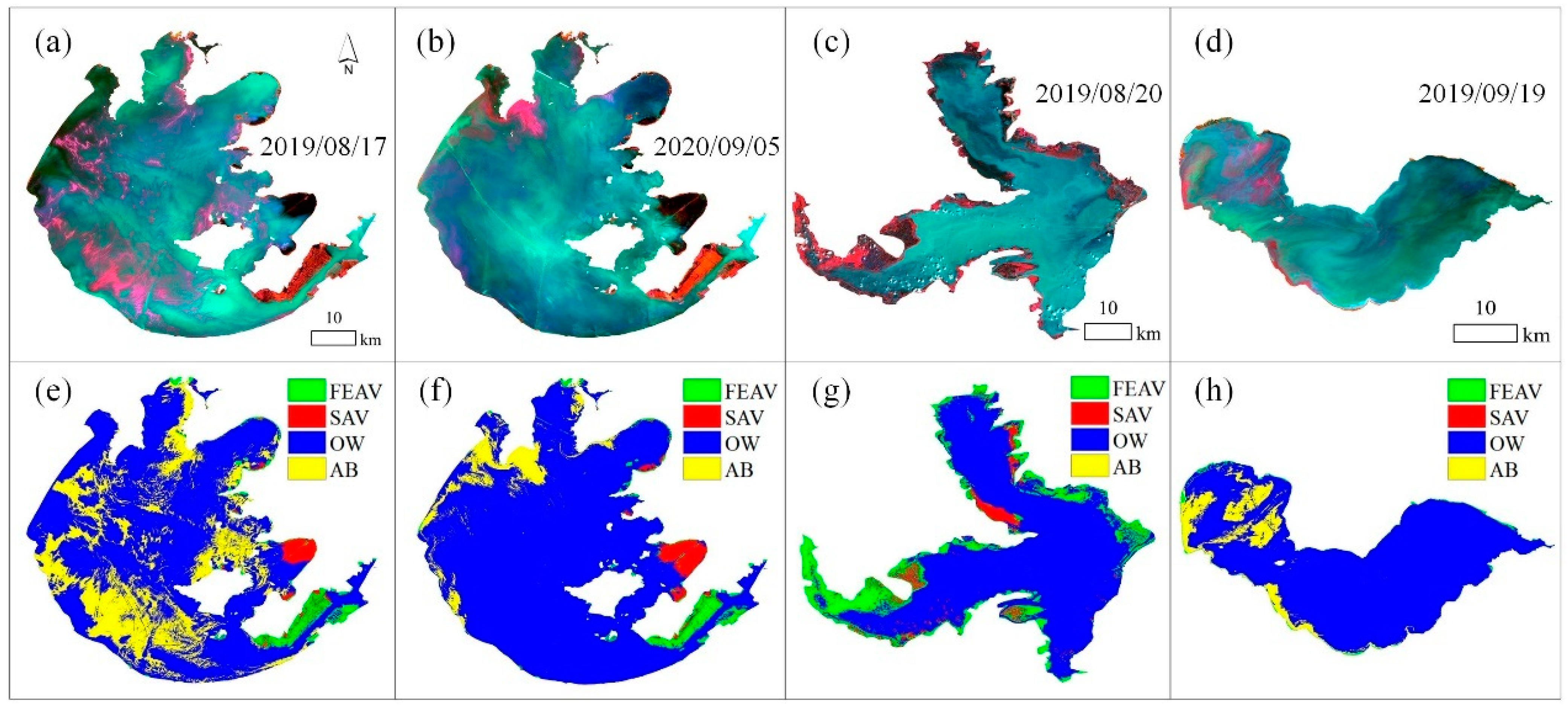
4.1.3. Comparison with Published Maps
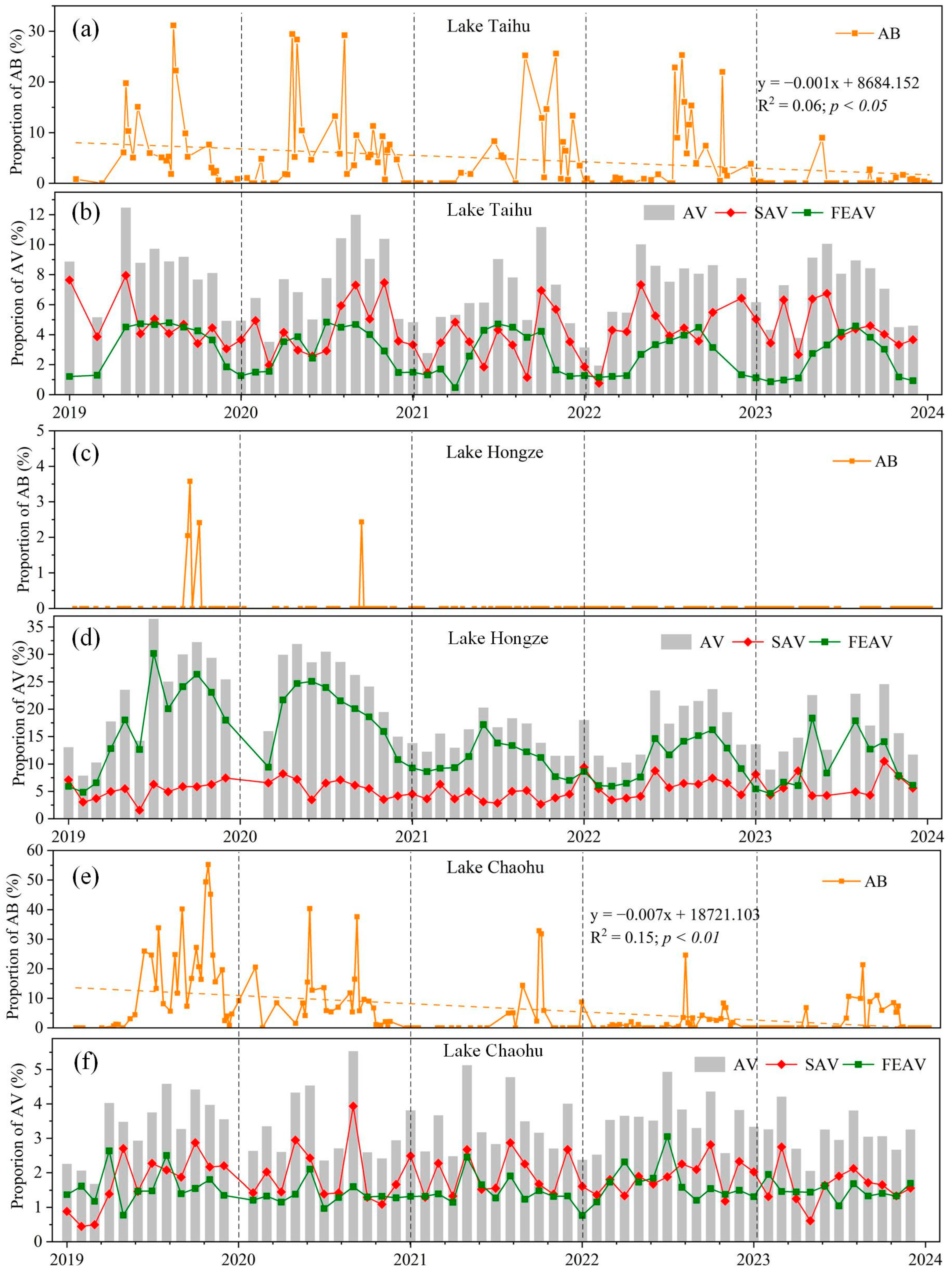
4.2. Algorithm Applications
5. Discussion
5.1. Advantages
5.2. Limitations
5.3. Implications
6. Conclusions
Supplementary Materials
Author Contributions
Funding
Data Availability Statement
Conflicts of Interest
References
- Kosten, S.; Piñeiro, M.; de Goede, E.; de Klein, J.; Lamers, L.P.M.; Ettwig, K. Fate of Methane in Aquatic Systems Dominated by Free-Floating Plants. Water Res. 2016, 104, 200–207. [Google Scholar] [CrossRef]
- Zeng, Q.; Wei, Z.; Yi, C.; He, Y.; Luo, M. The Effect of Different Coverage of Aquatic Plants on the Phytoplankton and Zooplankton Community Structures: A Study Based on a Shallow Macrophytic Lake. Aquat. Ecol. 2022, 56, 1347–1358. [Google Scholar] [CrossRef]
- Zhang, X. Effects of Benthic-Feeding Common Carp and Filter-Feeding Silver Carp on Benthic-Pelagic Coupling: Implications for Shallow Lake Management. Ecol. Eng. 2016, 88, 256–264. [Google Scholar] [CrossRef]
- Janssen, A.B.G.; Hilt, S.; Kosten, S.; De Klein, J.J.M.; Paerl, H.W.; Van De Waal, D.B. Shifting States, Shifting Services: Linking Regime Shifts to Changes in Ecosystem Services of Shallow Lakes. Freshw. Biol. 2021, 66, 1–12. [Google Scholar] [CrossRef]
- Hou, X.; Feng, L.; Dai, Y.; Hu, C.; Gibson, L.; Tang, J.; Lee, Z.; Wang, Y.; Cai, X.; Liu, J.; et al. Global Mapping Reveals Increase in Lacustrine Algal Blooms over the Past Decade. Nat. Geosci. 2022, 15, 130–134. [Google Scholar] [CrossRef]
- Zhang, Y.; Jeppesen, E.; Liu, X.; Qin, B.; Shi, K.; Zhou, Y.; Thomaz, S.M.; Deng, J. Global Loss of Aquatic Vegetation in Lakes. Earth-Sci. Rev. 2017, 173, 259–265. [Google Scholar] [CrossRef]
- Liu, D.; Ding, H.; Han, X.; Lang, Y.; Chen, W. Mapping Algal Blooms in Aquatic Ecosystems Using Long-Term Landsat Data: A Case Study of Yuqiao Reservoir from 1984–2022. Remote Sens. 2023, 15, 4317. [Google Scholar] [CrossRef]
- Oyama, Y.; Matsushita, B.; Fukushima, T. Distinguishing Surface Cyanobacterial Blooms and Aquatic Macrophytes Using Landsat/TM and ETM + Shortwave Infrared Bands. Remote Sens. Environ. 2015, 157, 35–47. [Google Scholar] [CrossRef]
- Qing, S.; Runa, A.; Shun, B.; Zhao, W.; Bao, Y.; Hao, Y. Distinguishing and Mapping of Aquatic Vegetations and Yellow Algae Bloom with Landsat Satellite Data in a Complex Shallow Lake, China during 1986–2018. Ecol. Indic. 2020, 112, 106073. [Google Scholar] [CrossRef]
- Luo, J.; Ni, G.; Zhang, Y.; Wang, K.; Shen, M.; Cao, Z.; Qi, T.; Xiao, Q.; Qiu, Y.; Cai, Y.; et al. A New Technique for Quantifying Algal Bloom, Floating/Emergent and Submerged Vegetation in Eutrophic Shallow Lakes Using Landsat Imagery. Remote Sens. Environ. 2023, 287, 113480. [Google Scholar] [CrossRef]
- Xu, D.; Pu, Y.; Zhu, M.; Luan, Z.; Shi, K. Automatic Detection of Algal Blooms Using Sentinel-2 MSI and Landsat OLI Images. IEEE J. Sel. Top. Appl. Earth Obs. Remote Sens. 2021, 14, 8497–8511. [Google Scholar] [CrossRef]
- Xin, Y.; Luo, J.; Xu, Y.; Sun, Z.; Qi, T.; Shen, M.; Qiu, Y.; Xiao, Q.; Huang, L.; Zhao, J.; et al. SSAVI-GMM: An Automatic Algorithm for Mapping Submerged Aquatic Vegetation in Shallow Lakes Using Sentinel-1 SAR and Sentinel-2 MSI Data. IEEE Trans. Geosci. Remote Sens. 2024, 62, 4416610. [Google Scholar] [CrossRef]
- Gao, H.; Li, R.; Shen, Q.; Yao, Y.; Shao, Y.; Zhou, Y.; Li, W.; Li, J.; Zhang, Y.; Liu, M. Deep-Learning-Based Automatic Extraction of Aquatic Vegetation from Sentinel-2 Images—A Case Study of Lake Honghu. Remote Sens. 2024, 16, 867. [Google Scholar] [CrossRef]
- Pu, J.; Song, K.; Lv, Y.; Liu, G.; Fang, C.; Hou, J.; Wen, Z. Distinguishing Algal Blooms from Aquatic Vegetation in Chinese Lakes Using Sentinel 2 Image. Remote Sens. 2022, 14, 1988. [Google Scholar] [CrossRef]
- Rodríguez-Garlito, E.C.; Paz-Gallardo, A.; Plaza, A. Mapping Invasive Aquatic Plants in Sentinel-2 Images Using Convolutional Neural Networks Trained with Spectral Indices. IEEE J. Sel. Top. Appl. Earth Obs. Remote Sens. 2023, 16, 2889–2899. [Google Scholar] [CrossRef]
- Yan, K.; Li, J.; Zhao, H.; Wang, C.; Hong, D.; Du, Y.; Mu, Y.; Tian, B.; Xie, Y.; Yin, Z.; et al. Deep Learning-Based Automatic Extraction of Cyanobacterial Blooms from Sentinel-2 MSI Satellite Data. Remote Sens. 2022, 14, 4763. [Google Scholar] [CrossRef]
- Song, B.; Park, K. Detection of Aquatic Plants Using Multispectral UAV Imagery and Vegetation Index. Remote Sens. 2020, 12, 387. [Google Scholar] [CrossRef]
- Kislik, C.; Dronova, I.; Grantham, T.E.; Kelly, M. Mapping Algal Bloom Dynamics in Small Reservoirs Using Sentinel-2 Imagery in Google Earth Engine. Ecol. Indic. 2022, 140, 109041. [Google Scholar] [CrossRef]
- Luo, J.; Ma, R.; Duan, H.; Hu, W.; Zhu, J.; Huang, W.; Lin, C. A New Method for Modifying Thresholds in the Classification of Tree Models for Mapping Aquatic Vegetation in Taihu Lake with Satellite Images. Remote Sens. 2014, 6, 7442–7462. [Google Scholar] [CrossRef]
- Ying, A.; Yonghong, B.; Zhengyu, H. Response of Predominant Phytoplankton Species to Anthropogenic Impacts in Lake Taihu. J. Freshw. Ecol. 2015, 30, 99–112. [Google Scholar] [CrossRef]
- Wang, H.; Zhang, X.; Peng, Y.; Wang, H.; Wang, X.; Song, J.; Fei, G. Restoration of Aquatic Macrophytes with the Seed Bank Is Difficult in Lakes with Reservoir-like Water-Level Fluctuations: A Case Study of Chaohu Lake in China. Sci. Total Environ. 2022, 813, 151860. [Google Scholar] [CrossRef]
- Gargiulo, M.; Dell’Aglio, D.A.G.; Iodice, A.; Riccio, D.; Ruello, G. Integration of Sentinel-1 and Sentinel-2 Data for Land Cover Mapping Using W-Net. Sensors 2020, 20, 2969. [Google Scholar] [CrossRef]
- Rao, P.; Zhou, W.; Bhattarai, N.; Srivastava, A.K.; Singh, B.; Poonia, S.; Lobell, D.B.; Jain, M. Using Sentinel-1, Sentinel-2, and Planet Imagery to Map Crop Type of Smallholder Farms. Remote Sens. 2021, 13, 1870. [Google Scholar] [CrossRef]
- Lee, J.-S.; Wen, J.-H.; Ainsworth, T.L.; Chen, K.-S.; Chen, A.J. Improved Sigma Filter for Speckle Filtering of SAR Imagery. IEEE Trans. Geosci. Remote Sens. 2009, 47, 202–213. [Google Scholar] [CrossRef]
- Messager, M.L.; Lehner, B.; Grill, G.; Nedeva, I.; Schmitt, O. Estimating the Volume and Age of Water Stored in Global Lakes Using a Geo-Statistical Approach. Nat. Commun. 2016, 7, 13603. [Google Scholar] [CrossRef] [PubMed]
- Pohl, C.; Van Genderen, J.L. Review Article Multisensor Image Fusion in Remote Sensing: Concepts, Methods and Applications. Int. J. Remote Sens. 1998, 19, 823–854. [Google Scholar] [CrossRef]
- Wang, Z.; Ziou, D.; Armenakis, C.; Li, D.; Li, Q. A Comparative Analysis of Image Fusion Methods. IEEE Trans. Geosci. Remote Sens. 2005, 43, 1391–1402. [Google Scholar] [CrossRef]
- Kim, Y.; Van Zyl, J. Comparison of Forest Parameter Estimation Techniques Using SAR Data. In Proceedings of the IGARSS 2001, Scanning the Present and Resolving the Future. Proceedings, IEEE 2001 International Geoscience and Remote Sensing Symposium (Cat. No.01CH37217), Sydney, NSW, Australia, 9–13 July 2001; Volume 3, pp. 1395–1397. [Google Scholar]
- Pelleg, D.; Moore, A. X-Means: Extending K-Means with E Cient Estimation of the Number of Clusters. In Proceedings of the Seventeenth International Conference on Machine Learning (ICML 2000), Standord, CA, USA, 29 June–2 July 2000; pp. 727–734. [Google Scholar]
- Abdi, H.; Williams, L.J. Principal Component Analysis. Wiley Interdiscip. Rev. Comput. Stat. 2010, 2, 433–459. [Google Scholar] [CrossRef]
- Ghoussein, Y.; Faour, G.; Fadel, A.; Haury, J.; Abou-Hamdan, H.; Nicolas, H. Hyperspectral Discrimination of Eichhornia Crassipes Covers, in the Red Edge and near Infrared in a Mediterranean River. Biol. Invasions 2023, 25, 3619–3635. [Google Scholar] [CrossRef]
- Jie, L.; Wang, J. Research on the Extraction Method of Coastal Wetlands Based on Sentinel-2 Data. Mar. Environ. Res. 2024, 198, 106429. [Google Scholar] [CrossRef]
- Luo, J.; Li, X.; Ma, R.; Li, F.; Duan, H.; Hu, W.; Qin, B.; Huang, W. Applying Remote Sensing Techniques to Monitoring Seasonal and Interannual Changes of Aquatic Vegetation in Taihu Lake, China. Ecol. Indic. 2016, 60, 503–513. [Google Scholar] [CrossRef]
- Liang, S.; Gong, Z.; Wang, Y.; Zhao, J.; Zhao, W. Accurate Monitoring of Submerged Aquatic Vegetation in a Macrophytic Lake Using Time-Series Sentinel-2 Images. Remote Sens. 2022, 14, 640. [Google Scholar] [CrossRef]
- Ostu, N. A Threshold Selection Method from Gray-Level Histograms. IEEE Trans. SMC 1979, 9, 62. [Google Scholar]
- Congalton, R.G. A Review of Assessing the Accuracy of Classifications of Remotely Sensed Data. Remote Sens. Environ. 1991, 37, 35–46. [Google Scholar] [CrossRef]
- Luo, J.; Duan, H.; Ma, R.; Jin, X.; Li, F.; Hu, W.; Shi, K.; Huang, W. Mapping Species of Submerged Aquatic Vegetation with Multi-Seasonal Satellite Images and Considering Life History Information. Int. J. Appl. Earth Obs. Geoinf. 2017, 57, 154–165. [Google Scholar] [CrossRef]
- Congalton, R.G. Assessing Landsat Classification Accuracy Using Discrete Multivariate Analysis Statistical Techniques. Photogramm. Eng. 1983, 49, 1671–1678. [Google Scholar]
- Jia, M.; Wang, Z.; Wang, C.; Mao, D.; Zhang, Y. A New Vegetation Index to Detect Periodically Submerged Mangrove Forest Using Single-Tide Sentinel-2 Imagery. Remote Sens. 2019, 11, 2043. [Google Scholar] [CrossRef]
- Thamaga, K.H.; Dube, T. Understanding Seasonal Dynamics of Invasive Water Hyacinth (Eichhornia crassipes) in the Greater Letaba River System Using Sentinel-2 Satellite Data. GIScience Remote Sens. 2019, 56, 1355–1377. [Google Scholar] [CrossRef]
- Hou, X.; Feng, L.; Chen, X.; Zhang, Y. Dynamics of the Wetland Vegetation in Large Lakes of the Yangtze Plain in Response to Both Fertilizer Consumption and Climatic Changes. ISPRS J. Photogramm. Remote Sens. 2018, 141, 148–160. [Google Scholar] [CrossRef]
- Alahuhta, J.; Lindholm, M.; Baastrup-Spohr, L.; García-Girón, J.; Toivanen, M.; Heino, J.; Murphy, K. Macroecology of Macrophytes in the Freshwater Realm: Patterns, Mechanisms and Implications. Aquat. Bot. 2021, 168, 103325. [Google Scholar] [CrossRef]
- Thomaz, S.M. Ecosystem Services Provided by Freshwater Macrophytes. Hydrobiologia 2023, 850, 2757–2777. [Google Scholar] [CrossRef]
- Regnier, P.; Resplandy, L.; Najjar, R.G.; Ciais, P. The Land-to-Ocean Loops of the Global Carbon Cycle. Nature 2022, 603, 401–410. [Google Scholar] [CrossRef] [PubMed]
- Roth, F.; Broman, E.; Sun, X.; Bonaglia, S.; Nascimento, F.; Prytherch, J.; Brüchert, V.; Lundevall Zara, M.; Brunberg, M.; Geibel, M.C.; et al. Methane Emissions Offset Atmospheric Carbon Dioxide Uptake in Coastal Macroalgae, Mixed Vegetation and Sediment Ecosystems. Nat. Commun. 2023, 14, 42. [Google Scholar] [CrossRef]
- Shen, C.; Qian, M.; Song, Y.; Chen, B.; Yang, J. Surface pCO2 and Air-Water CO2 Fluxes Dominated by Submerged Aquatic Vegetation: Implications for Carbon Flux in Shallow Lakes. J. Environ. Manag. 2024, 370, 122839. [Google Scholar] [CrossRef] [PubMed]
- Peixoto, R.B.; Marotta, H.; Bastviken, D.; Enrich-Prast, A. Floating Aquatic Macrophytes Can Substantially Offset Open Water CO2 Emissions from Tropical Floodplain Lake Ecosystems. Ecosystems 2016, 19, 724–736. [Google Scholar] [CrossRef]
- Qi, T.; Xiao, Q.; Cao, Z.; Shen, M.; Ma, J.; Liu, D.; Duan, H. Satellite Estimation of Dissolved Carbon Dioxide Concentrations in China’s Lake Taihu. Environ. Sci. Technol. 2020, 54, 13709–13718. [Google Scholar] [CrossRef]
- Ran, L.; Butman, D.E.; Battin, T.J.; Yang, X.; Tian, M.; Duvert, C.; Hartmann, J.; Geeraert, N.; Liu, S. Substantial Decrease in CO2 Emissions from Chinese Inland Waters Due to Global Change. Nat. Commun. 2021, 12, 1730. [Google Scholar] [CrossRef]


| Lake Name | Survey Date | Image Date | SAV Samples | FEAV Samples | AB Samples | OW Samples |
|---|---|---|---|---|---|---|
| Taihu | 17 August 2019 | 17 August 2019 | 624 | 1445 | 1368 | 356 |
| 5 September 2020 | 5 September 2020 | 596 | 1533 | 1107 | 333 | |
| Chaohu | 15 September 2019 | 19 September 2019 | 74 | 100 | 293 | 108 |
| Hongze | 24 August 2019 | 20 August 2019 | 110 | 281 | / | 202 |
| 25 August 2019 | ||||||
| Total | / | / | 1404 | 3359 | 2768 | 999 |
| Lake Name/ Image Date | Measured Class | |||||||
|---|---|---|---|---|---|---|---|---|
| Taihu 17 August 2019 | SAV | FEAV | AB | OW | Sum | UA (%) | ||
| Map class | SAV | 208 | 4 | 12 | 9 | 233 | 89.27 | |
| FEAV | 11 | 454 | 29 | 0 | 494 | 91.9 | ||
| AB | 21 | 27 | 406 | 17 | 471 | 86.19 | ||
| OW | 14 | 0 | 21 | 330 | 365 | 90.41 | ||
| Sum | 254 | 485 | 468 | 356 | 1563 | |||
| PA (%) | 81.89 | 93.61 | 86.75 | 92.7 | ||||
| OA = 89.44%; Kappa = 0.86 | ||||||||
| Taihu 5 September 2020 | SAV | FEAV | AB | OW | Sum | UA (%) | ||
| Map class | SAV | 319 | 7 | 13 | 2 | 341 | 93.55 | |
| FEAV | 8 | 489 | 17 | 0 | 514 | 95.13 | ||
| AB | 9 | 22 | 329 | 19 | 379 | 86.81 | ||
| OW | 11 | 0 | 23 | 312 | 346 | 90.17 | ||
| Sum | 347 | 518 | 382 | 333 | 1580 | |||
| PA (%) | 91.92 | 94.4 | 86.13 | 93.69 | ||||
| OA = 91.72%; Kappa = 0.89 | ||||||||
| Chaohu 19 September 2019 | SAV | FEAV | AB | OW | Sum | UA (%) | ||
| Map class | SAV | 71 | 2 | 1 | 0 | 74 | 95.95 | |
| FEAV | 0 | 90 | 0 | 0 | 90 | 100 | ||
| AB | 3 | 8 | 279 | 16 | 306 | 91.18 | ||
| OW | 0 | 0 | 13 | 92 | 105 | 87.62 | ||
| Sum | 74 | 100 | 293 | 108 | 575 | |||
| PA (%) | 95.95 | 90 | 95.22 | 85.19 | ||||
| OA = 82.61%; Kappa = 0.73 | ||||||||
| Hongze 20 August 2019 | SAV | FEAV | AB | OW | Sum | UA (%) | ||
| Map class | SAV | 103 | 6 | \ | 2 | 111 | 92.79 | |
| FEAV | 1 | 272 | \ | 0 | 273 | 99.63 | ||
| AB | \ | \ | \ | \ | \ | \ | ||
| OW | 6 | 3 | \ | 200 | 209 | 95.69 | ||
| Sum | 110 | 281 | \ | 202 | 593 | |||
| PA (%) | 93.64 | 96.8 | \ | 99.01 | ||||
| OA = 86.84%; Kappa = 0.79 | ||||||||
Disclaimer/Publisher’s Note: The statements, opinions and data contained in all publications are solely those of the individual author(s) and contributor(s) and not of MDPI and/or the editor(s). MDPI and/or the editor(s) disclaim responsibility for any injury to people or property resulting from any ideas, methods, instructions or products referred to in the content. |
© 2025 by the authors. Licensee MDPI, Basel, Switzerland. This article is an open access article distributed under the terms and conditions of the Creative Commons Attribution (CC BY) license (https://creativecommons.org/licenses/by/4.0/).
Share and Cite
Xin, Y.; Luo, J.; Zhai, J.; Wang, K.; Xu, Y.; Qin, H.; Chen, C.; You, B.; Cao, Q. An Automatic Algorithm for Mapping Algal Blooms and Aquatic Vegetation Using Sentinel-1 SAR and Sentinel-2 MSI Data. Land 2025, 14, 592. https://doi.org/10.3390/land14030592
Xin Y, Luo J, Zhai J, Wang K, Xu Y, Qin H, Chen C, You B, Cao Q. An Automatic Algorithm for Mapping Algal Blooms and Aquatic Vegetation Using Sentinel-1 SAR and Sentinel-2 MSI Data. Land. 2025; 14(3):592. https://doi.org/10.3390/land14030592
Chicago/Turabian StyleXin, Yihao, Juhua Luo, Jinlong Zhai, Kang Wang, Ying Xu, Haitao Qin, Chao Chen, Bensheng You, and Qing Cao. 2025. "An Automatic Algorithm for Mapping Algal Blooms and Aquatic Vegetation Using Sentinel-1 SAR and Sentinel-2 MSI Data" Land 14, no. 3: 592. https://doi.org/10.3390/land14030592
APA StyleXin, Y., Luo, J., Zhai, J., Wang, K., Xu, Y., Qin, H., Chen, C., You, B., & Cao, Q. (2025). An Automatic Algorithm for Mapping Algal Blooms and Aquatic Vegetation Using Sentinel-1 SAR and Sentinel-2 MSI Data. Land, 14(3), 592. https://doi.org/10.3390/land14030592