Abstract
Land-use change models are used to predict future land-use scenarios. Various methods for predicting changes can be found in the literature, which can be divided into two groups: baseline models and machine-learning-based models. Baseline models use clear change logics, such as proximity or distance from spatial objects. While machine-learning-based models use computational methods and spatial variables to identify patterns that explain the occurrence of changes. Considering these two groups of models, machine-learning-based models are much more widely used, even though their formulation is considerably more complex. However, the lack of studies comparing the performance of models from these two groups makes it impossible to determine the superiority of one over the other. Therefore, this article aims to evaluate and compare the accuracy of baseline and machine-learning-based models for study areas in three Brazilian biomes. Four baseline models (Euclidean distance from anthropic uses, Euclidean distance from vegetation suppressions, null change model, and random change model) and four machine-learning-based models (TerrSet artificial neural network, TerrSet SimWeigth, Weights of Evidence–Dinamica Ego. and Random Forest model) were trained considering the environmental context of the period from 1995 to 2000. The objective was to predict natural vegetation suppression from 2000 to the years 2005, 2010, 2015, and 2020. The predicted maps were evaluated by comparing them with reference land-use maps using rigorous accuracy methods. The results show that, regardless of the underlying method, the models presented similar performance in all situations. The results and discussions provide a contribution to understanding the strengths and weaknesses of various change models in different environmental contexts.
1. Introduction
Land-use change models are employed in various scientific fields to predict expected future alterations [1,2]. The development of such models is based on the identification of patterns and transition rates between time points t0 and t1, and then the prediction of changes from t1 to tx [3]. Two groups of modeling methods can be cited: statistical models, commonly based on machine learning methods; and baseline models, generally based on Euclidean distance surfaces [4,5,6,7].
To formulate machine-learning-based models, a training process is required using samples of changes and persistence of land-use that occurred between time points t0 and t1, and spatial predictive variables with the ability to explain the phenomenon. For each sample, information contained in the explanatory variables is extracted. Then, a machine learning method is used to identify the characteristics that differentiate samples of change and of persistence. As a result, a probabilistic surface is generated, indicating the probability to land-use change. Examples of machine-learning-based approaches include the software TerrSet, Clue-S, Dinamica EGO, and programs based on computational language [4,5,8].
Baseline models do not require a training process. Instead, the probability surface is usually produced by some calculation, as the Euclidean distance from a spatial object that can explain the land-use change. The proximity or distance from this object determines the probability of change. This approach is frequently used for comparison with the outputs of machine-learning-based models. Examples of baseline models include Euclidean distance from vegetation suppression and urban uses [7,9].
In both methods, after creating the probability surface, it is necessary to apply a change allocation algorithm to predict the future land-use map. Cellular automata algorithms are commonly used in this step. Equation (1) describes the generic operation of this type of algorithm.
where Stxij represents the state of cell ij at time tx; f is the transition function; St1ij refers to the state of cell ij at time t1; Ωt1ij is the neighborhood function of cell ij at time t1; C represents the transition constraints; N represents the number of neighboring cells considered [7].
The use of cellular automata, which integrates the neighborhood context, is considered to be more effective than simply allocating changes in cells classified as the most susceptible by the model. This is due to the fact that changes occur in a landscape context, where transformed cells are influenced by their neighborhood during the process. In this sense, some of the land-use changes being predicted could be explained by the expansion or reduction in a specific class through contact [4].
In addition to model formulation, accuracy assessment is an essential step. Only through this can the predictive capacity to explain the modeled changes be estimated. Several methods are available for this purpose. Some approaches provide detailed information about the predictions, while others may offer potentially misleading results [3,6,9,10,11,12,13]. When investigating recent work, it is observed that some accuracy assessment methods continue to be used despite having been described as potentially misleading many times [1,2].
Given the characteristics of the models, machine-learning-based models are expected to perform considerably better than baseline models. This is justified by the greater complexity of their formulation and the use of training methods. Despite this hypothesis, there is a lack of studies that compare the performance of machine-learning-based and baseline models. In this sense, the main objective of this study was to assess whether machine-learning-based models are really more accurate than baseline models. Additionally, comparisons are made between the accuracy assessment methods used in this study and the methods generally used in this field of research.
The results of this article aim to contribute to the scientific community by providing a foundation for comparing the performance of baseline and machine-learning-based land-use change models.
2. Materials and Methods
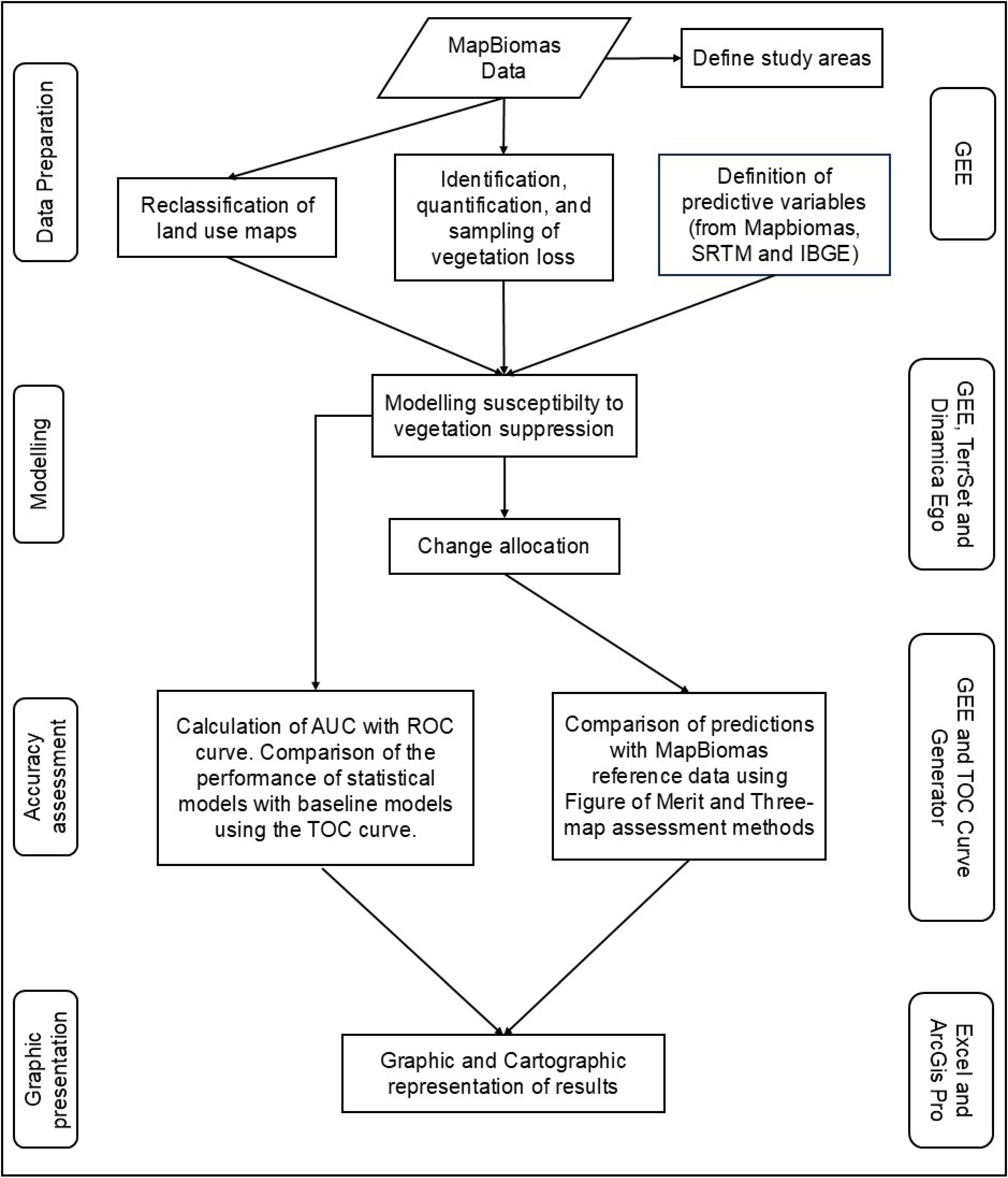
This study evaluated the performance of eight land-use change models (four baseline and four machine-learning-based) in selected areas of three Brazilian biomes. The models were used to predict the occurrence of vegetation suppression using a one-way approach. The training was conducted for the period from 1995 to 2000, while prediction maps were made for the periods from 2000 to 2005, 2010, 2015 and 2020. Figure 1 presents the workflow of the methodology. In the central part of the figure are the processes carried out, on the left are the stages of the work, and on the right are the software used. All the computer codes used are presented in the Supplementary Materials.

Figure 1.
Methodology flowchart.
2.1. Study Area
The study areas were selected to represent different environmental contexts that experienced land-use changes and the suppression of natural vegetation between 2000 and 2020. In three Brazilian biomes, areas were selected that exhibited major land-use changes during this period. The areas were chosen based on land-use maps from collection 8 of the MAPBIOMAS project [14] and the tiles of the respective 1:250,000 grid.
We first calculated the area of the natural vegetation classes for the years 2000 and 2020 in each grid cell of the map. Subsequently, we calculated the difference in the area of these vegetation formations between 2000 and 2020. Finally, we chose the grid cell with the largest absolute reduction in natural vegetation cover during the analyzed period in the Amazon, Cerrado, and Pampa biomes. As land-use changes are typically rare occurrences when compared to persistence, the selection of grids with high rates of change aimed to ensure that all prediction periods could present enough change for comparison with the reference data. Furthermore, the selection of areas in three different biomes sought to represent different environmental characteristics and pressures that may affect change.
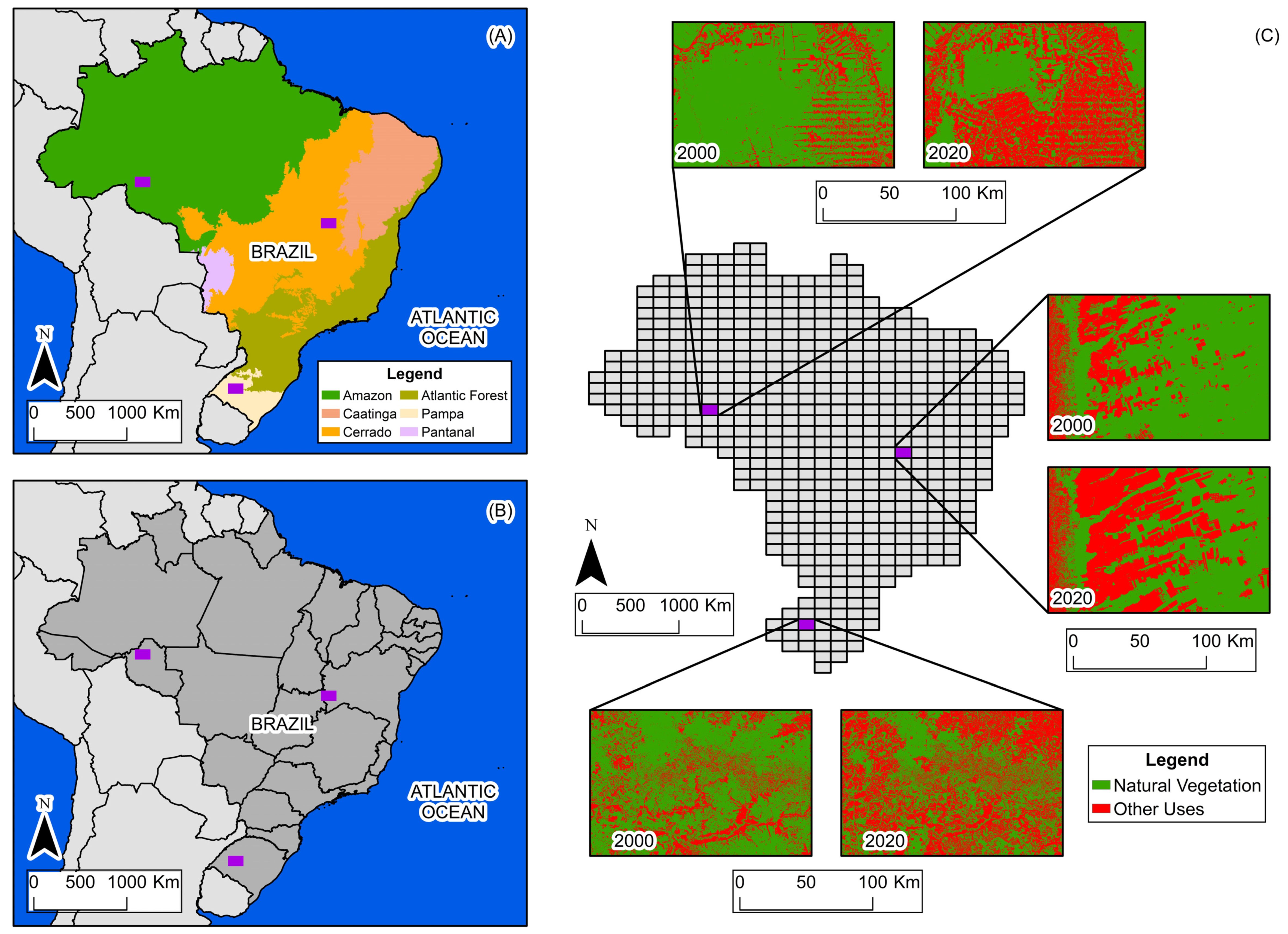
The selected study areas encompass a wide variety of spaces and dynamics of land-use change. Figure 2 shows the location of the three study areas.
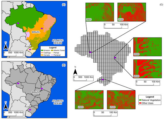
Figure 2.
(A) Biome boundaries and study areas. (B) State boundaries and study areas. (C) Grid, study areas, and land use and land cover in 2000 and 2020.
The Amazon biome study area is located in the state of Rondônia, in northern Brazil, within the longitudinal range of 64°30′ W to 63° W, and the latitudinal range of 9° S to 10° S. It is characterized by the predominance of dense, humid tropical forest, contrasting with extensive areas of pasture derived from recent deforestation. In the period from 2000 to 2020, there was a reduction of approximately 40% in the natural vegetation cover, with deforestation advancing from south to north. The suppression of the Amazon rainforest is primarily driven by timber harvesting and the expansion of livestock and agricultural production. Today, this process is regarded as a global environmental issue, attracting attention from various sectors of society [14].
The Cerrado biome study area is located on the border of the states of Bahia and Goiás, in the central portion of Brazil, within the longitudinal range of 46°30′ W to 45° W, and the latitudinal range of 13° S to 14° S. It is characterized by mosaics of savannah, grassland, agriculture, and pasture. In the period from 2000 to 2020, there was a reduction of approximately 28% in the natural vegetation cover, with suppression progressing from west to east. The reduction in natural vegetation in this part of Cerrado is motivated by the implementation of large-scale monocultures, a process that has received attention from the scientific community in order to understand its environmental impacts [14,15].
The Pampa biome study area is located in the state of Rio Grande do Sul, in southern Brazil, within the longitudinal range of 55°30′ W to 54° W, and the latitudinal range of 29° S to 30° S. It is characterized by grassland vegetation, pastures, agricultural uses, and forested areas. Between 2000 and 2020, natural vegetation decreased by approximately 29%, with suppression occurring without a defined spatial pattern. The conversion of natural vegetation in this part of Pampa is primarily driven by the establishment of agricultural crops, particularly the shift from grassland formations to soybean plantations. Between 2000 and 2020, soybean production expanded extensively in the biome, considerably altering the landscape. Another important process is the periodic alternation of land-use classes, with transitions from grassland vegetation to pasture and rice production, and vice versa [14].
2.2. Data Used
All the geospatial data used in this study come from open sources and are accessible for consultation. The land-use maps were derived from the MAPBIOMAS project, a collaborative effort involving researchers from various institutions in Brazil, including universities, NGOs, research institutes, and technology start-ups. One of its main products is the annual land-use and land-cover maps, available since 1985 for the entire Brazilian territory. These maps are generated using data from the Landsat program, offering a spatial resolution of 30 m. A key strength of this mapping is robust accuracy assessment, allowing users to understand the disagreements in the classification for each land-use class mapped [14,16].
The altitude and slope data were derived from the NASADEM digital elevation model. NASADEM is a product resulting from the reprocessing of the Radar Shuttle Topographic Mission (SRTM) with a spatial resolution of 30 m. Compared to SRTM, NASADEM provides greater accuracy due to processing improvements and the incorporation of auxiliary data from the Advanced Spaceborne Thermal Emission and Reflection Radiometer (ASTER) and the Ice, Cloud, and Land Elevation Satellite (ICESat)/Geoscience Laser Altimeter System (GLAS) [17].
The road network was derived from the Brazilian Institute of Geography and Statistics (IBGE), representing federal and state roads. The scale of these data is 1:250,000, and the features were delimited using images from the Sentinel-2, Planet, and Maxar sensors. During the validation of the product, an average positional error of 125 m was considered acceptable [18].
2.3. Data Preparation
The data preparation process was divided into three main stages: (1) reclassification of land-use maps from the MapBiomas project; (2) identification, quantification, and sampling of natural vegetation loss; and (3) definition of predictive variables for modeling.
2.3.1. Reclassification of Land-Use Maps from the MapBiomas Project
The reclassification of land-use maps from the MapBiomas project was performed with the aim of grouping the original classes into only two: natural vegetation and other uses. For the reclassification, land-use maps from the years 1995, 2000, 2005, 2010, 2015, and 2020 were selected. These years and time intervals were defined with the objective of the training period having the same duration as each prediction period, allowing the model’s results to be evaluated for prediction phases with equivalent time periods. Details of the reclassification process can be found in the Supplementary Materials.
2.3.2. Identification, Quantification, and Sampling of Vegetation Loss
The amount of change expected in the future was defined using the two land-use maps from the training period. From these maps, it is possible to identify and quantify the areas of vegetation suppression during the training, as well as allocate samples of change and of persistence. Equation (2) exemplifies this process as follows:
where the suppression of natural vegetation during the training period (SNVTP) is equal (=) to the difference (−) between the natural vegetation area in 1995 (NVAt0) and the natural vegetation area in 2000 (NVAt1). Knowing the size of the suppressed area in the training period and assuming that in the future the rate of suppression will remain the same, it is possible to predict the expected area of suppression for any period of time. Equation (3) presents this possibility.
where the future suppression of natural vegetation (FSNVx) is calculated (=) based on the total area of natural vegetation suppression during the training period (NVAt0 − NVAt1), divided (/) by the vegetation area in t0 (VAt0), and multiplied (·) by 1% of the vegetation area from the period preceding the extrapolation (100/VAtx). For example, if the model’s training occurred between 1995 and 2000 and it was identified that vegetation suppression during this period corresponded to 1% of the existing vegetation in 1995, to estimate the changes for the year 2005, 1% of the vegetation area in 2000 was used. For 2010, 1% of the estimated vegetation area for 2005 would be applied, and so on.
This method was used to estimate the expected changes in the baseline models and in the model using Random Forest. In the other models used, this step occurs automatically.
2.3.3. Definition of the Predictive Variables
The predictive variables for natural vegetation suppression were derived from MapBiomas, NASADEM, and IBGE data. From MapBiomas, we computed Euclidean distance from the water bodies in 1995, urban space in 1995, anthropogenic uses in 1995, and vegetation suppression between 1990 and 1995. From NASADEM we extracted altitude and slope data. And from the IBGE, we calculated Euclidean distance for the roads existing in 1995.
As the model training was carried out with samples of vegetation suppression between 1995 and 2000, the predictive variables cannot be correlated with the data from this period. Therefore, the training input variables derived from MapBiomas were created based on the 1995 land-use map or the vegetation suppressions that occurred in the preceding period (1990–1995). After the creation of the predictive variables, they were grouped into a data cube and, together with the land-use maps, served as input data for the modeling stage.
2.4. Modeling Probability to Vegetation Suppression
In the model development stage, we used three software and four methods: from the TerrSet software, the Artificial Neural Network and SimWeight methods were used; from the Dinamica EGO software, the weights of evidence method; and from the Google Earth Engine platform [19], the Random Forest method. These methods were selected due to their popularity and frequent use by the modeling community.
TerrSet is a geographic information system (GIS) developed by Clark University in 1987. Its applications encompass GIS analysis, remote sensing image processing, and spatial modeling. A new free version, TerrSet LiberaGIS V.20, was released in December 2024 [5].
DinamicaEGO is an environmental modeling platform developed by the Remote Sensing Center (CSR) of the Federal University of Minas Gerais (UFMG) in 2002. Its applications include land-use change modeling, urban expansion modeling, wildfire modeling, and biodiversity modeling [4].
Google Earth Engine is a free, cloud-based platform for processing remote sensing data using JavaScript. Its major advantages are free access, a massive collection of satellite imagery, cloud-based computing, and the opportunity to collaborate with others [19].
For the TerrSet and Dinamica Ego models, the required inputs were land-use maps from 1995 and 2000, and predictive variables. In these software programs, the creation of change and persistence samples; the calculation of transition rates during the training and prediction periods; and the allocation of changes by cellular automata are performed automatically. In the case of Google Earth Engine (GEE) and Random Forest, these steps were carried out through computer programming. Each of the four models is described in detail below.
2.4.1. TerrSet—Artificial Neural Network (ANN)
The ANN method used in the TerrSet software is inspired by the functioning of the human brain, with artificial neurons organized into layers (input, hidden, and output) for data processing. The architecture used is Multi-Layer Perceptron (MLP), adjusting the training data in relation to a validation set. Neurons are connected, and synaptic weights are adjusted by backpropagation to maximize convergence [8]. In this method, the user can define the number of samples used in each class and the number of iterations. In this study, 10,000 samples per class and 10,000 iterations were used.
2.4.2. TerrSet—SimWeight
The SimWeight method of the TerrSet software is an algorithm based on similarity-weighted instances. It simplifies land-use change modeling by requiring only two parameters: the number of training samples and the number of neighboring samples considered in the training process (parameter K). Using the K-Nearest Neighbor logic, for each cell to be evaluated, the k-nearest samples (change or persistence) are identified. Then, the distance in the variable space of each unknown location is calculated in relation to the change samples that are within the k interval. An exponential weighting function is then used to associate labels with the cells, indicating the potential for transition based on environmental similarity with altered locations. SimWeight generates a continuous probability surface using only change samples. This is based on the assumption that persistence samples are not effectively examples of locations that have not changed, only that they are known to be locations that have not yet changed [5]. In the modeling, the parameter K was adjusted to 100 neighboring samples, and 10,000 samples were used in training.
2.4.3. Dinamica Ego 7—Weights of Evidence
The evidence weights method used in the Dinamica EGO 7 software is a Bayesian approach where the probability of an event occurring is defined given a spatial pattern. The weights of evidence for land-use changes are determined by the ability of ranges of values of the predictive variables to distinguish between areas where changes occurred and where they did not. The land-use change probability surface is generated by summing the evidence weights that each cell received from all the spatial variables used [4]. In the Dinamica Ego software, the adjustment of evidence weights occurs automatically, not allowing any user definition.
2.4.4. Google Earth Engine—Random Forest
The Random Forest classifier employed in the GEE platform is a non-parametric algorithm capable of estimating values or assigning objects to classes without making assumptions about the spatial distribution or structure of the data. Using training samples and regression analysis, the classifier divides the samples into increasingly homogeneous subsets based on values extracted from explanatory variables. The parameter for subdivision is the selection of predictive attributes that minimize uncertainty. In a decision tree, a sample is classified by the mean of the subset where it is allocated in the regression analysis. Its final label in a Random Forest classification is the result of the classification in the various regression trees, being the value that has been repeated the most times [20,21,22].
In this method, 10,000 samples were used for each class (occurrence of natural vegetation suppression and non-occurrence) and 28 decision trees. The number of decision trees was determined following the principle of parsimony, aiming for the best possible performance at the lowest computational cost.
After generating the probability surface, a cellular automata algorithm was adapted for allocating the predicted changes. A simple multiplication was performed between the probability surface for vegetation suppression, a 5 × 5 neighborhood filter counting the number of pixels classified by MapBiomas as anthropogenic uses in 2000, and a surface with random values ranging from 0 to 1. Using the result of this multiplication, the pixels with the highest susceptibilities were selected based on the rates of change derived from Equation (2).
2.5. Baseline Models
We used four baseline models: Euclidean distance from anthropogenic uses in 2000, Euclidean distance from vegetation suppressions between 1995 and 2000, a surface with random values from 0 to 1, and the land-use map reclassified to natural vegetation and anthropic for the year 2000. As there is no training process in these models, there is no correlation problem when using land-use data from this period.
For the Euclidean distance from anthropogenic uses in 2000 and Euclidean distance from vegetation suppression occurring between 1995 and 2000, the lowest distance values were considered the most susceptible to vegetation suppression. For the surface with random values from 0 to 1, the highest values were considered the most susceptible. The 2000 land-use map was used as a null change model.
2.6. Accuracy Assessment
The accuracy assessment was divided into two stages, one for the probability surfaces and the other for the predicted maps. For the first, the objective was to measure the models’ ability to differentiate areas prone to suppression and persistence of natural vegetation during the prediction periods. For the predicted maps, the aim was to measure the ability of the models to correctly allocate the suppression of natural vegetation.
2.6.1. Accuracy Assessment of Probability Surfaces
The accuracy of probability surfaces was assessed using the ROC (Receiver Operating Characteristic) and TOC (Total Operating Characteristic) curve methods [6,11]. The ROC evaluates the rate of vegetation suppression samples correctly classified (true positives) and incorrectly classified (false positives) by the models for each probability level. The true positive rate was calculated using Equation (4), while the false positive rate by Equation (5).
where the true positive rate for each probability level (TPR) is obtained (=) by dividing (/) the quantity of true positives (TP) by the sum of true positives and false negatives (TP + FN). The false positive rate is obtained (=) by dividing (/) false positives (FP) by the sum of false positives and true positives (FP + TP). This approach is widely used to assess the accuracy of binary classifications, with applications in various fields of study [6].
The Area Under the Curve (AUC) is a way to summarize the ROC analysis by aggregating the value of true and false positive rates across all thresholds. In a model capable of perfectly differentiating all change and persistence samples, the AUC value would be 1. In contrast, for a model with performance equal to randomness, the AUC value would be 0.5.
The AUC calculation was performed on the GEE platform. For each prediction period, 10,000 samples of vegetation suppression and 10,000 samples of non-suppression were used. The probability surfaces were divided into 100 equal parts based on their histograms. For each of these parts, the true and false positive rates were then calculated. The AUC value was defined by the average performance of the models at each of the 100 thresholds.
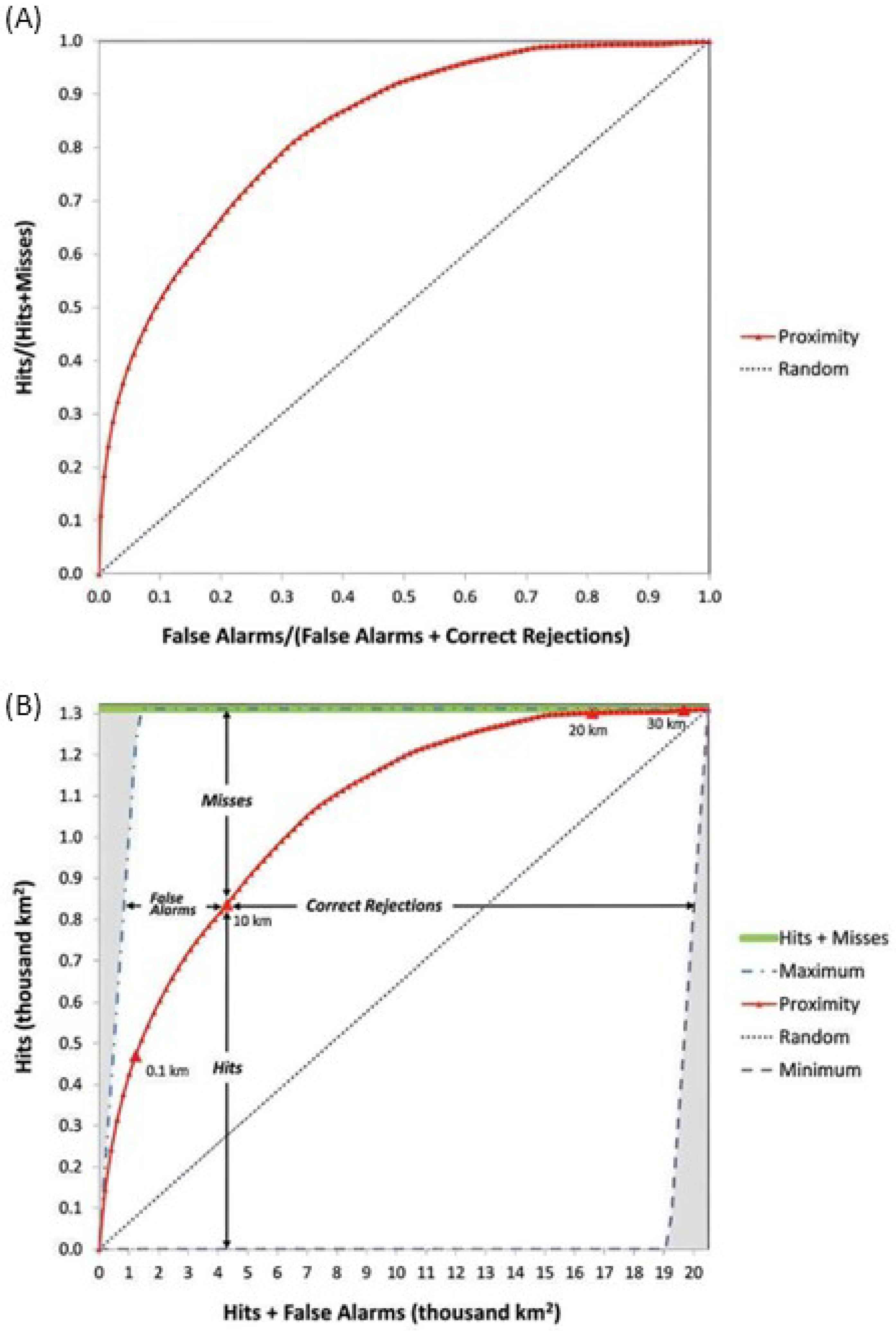
The TOC method was proposed as an improvement over the ROC. For each probability threshold, this approach allows for the quantification of hits, misses, false alarms, and correct rejections, thus providing more information than the ROC. Figure 3 presents the ROC and TOCs [11].
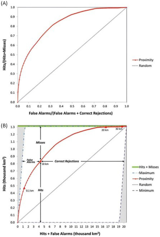
Figure 3.
(A) ROC and (B) TOC [11].
Unlike the ROC, which commonly presents hits and false alarms based on proportions of change and persistence samples, the TOC presents hits and false alarms in square kilometers. This occurs because the TOC calculation utilizes a reference map encompassing all changes and persistence within the prediction period, enabling the generation of area-based statistics. The y-axis of the TOC graphic shows the total amount of change that occurred between t0 and t1, while the X-axis represents the total area of the study area at t0 [11].
To generate the curves, we used the TOC Curve Generator v1.2.7 software [23]. The software requires the probability surface to be evaluated, a mask of the study area’s boundary, and the reference map of suppressions occurred during the prediction periods. The mask was composed by the natural vegetation cover of the year 2000, because only pixels in this area can undergo suppressions in the subsequent prediction periods. As done for the ROC, the probability surfaces were divided into 100 equal parts for the calculation of the true positive and false positive rates
2.6.2. Accuracy Assessment of the Predicted Maps
The accuracy assessment of the predicted maps was also conducted using two methods, a three-map comparison approach and the Figure of Merit [7,12]. In the former approach, using two reference maps at time states t1 and tx, plus the predicted maps for state tx, it is possible to quantify the components of agreement and disagreement of the prediction.
By comparing the reference maps at t1 and tx, the observed changes and persistence are identified. When comparing the reference map at t1 with the prediction result at tx, the areas predicted as changes by the model are obtained. In addition, by comparing the reference map at tx with the prediction result at tx, the overall accuracy of the model is computed. By analyzing these three comparisons together, it is possible to quantify the persistence correctly predicted by the model (areas where the model predicted persistence and the reference maps also showed persistence), false alarms (areas where the model predicted change, but in the reference there was persistence), misses (areas where the model predicted persistence, but the reference showed change), and hits (areas where the model predicted change, and the reference showed change).
This approach was implemented on the GEE platform using the reclassified land-use and land-cover maps from the MAPBIOMAS project as reference data. In addition to the components of agreement and disagreement, areas classified in the reference maps as other uses at t1 and as natural vegetation at tx were computed as regeneration; areas of anthropogenic uses at t1 that remained the same at tx were classified as excluded.
After calculating the area of the components derived from the three maps approach, the results were organized in Excel 16 software and presented as graphs.
Based on the area of the components mapped by the three-map comparison, the Figure of Merit was calculated using Equation (6).
where the Figure of Merit represents the proportion of hits relative to the sum of misses, hits, and false alarms [12]. This approach simplifies the comparison of model performance and focuses on areas of change, distinguishing itself from overall accuracy which includes correct rejections.
In addition, for each study area and prediction period, the model with the highest Figure of Merit was selected to be presented as a map. Due to the large number of results (96 maps resulting from the evaluation by three maps), it was not possible to present all the maps in the article.
3. Results
3.1. Accuracy Assessment of the Vegetation Suppression Probability Surfaces
Table 1 presents the AUC results found for the probability surfaces of the study area in the Amazon biome. It is observed that the value obtained for the baseline models is higher than that obtained for the machine-learning-based models in all prediction periods. Among these models, Random Forest (RF) achieved the best performance, while the Sim Weight—TerrSet obtained the lowest AUC value.

Table 1.
AUC values of the models for the study area in the Amazon biome.
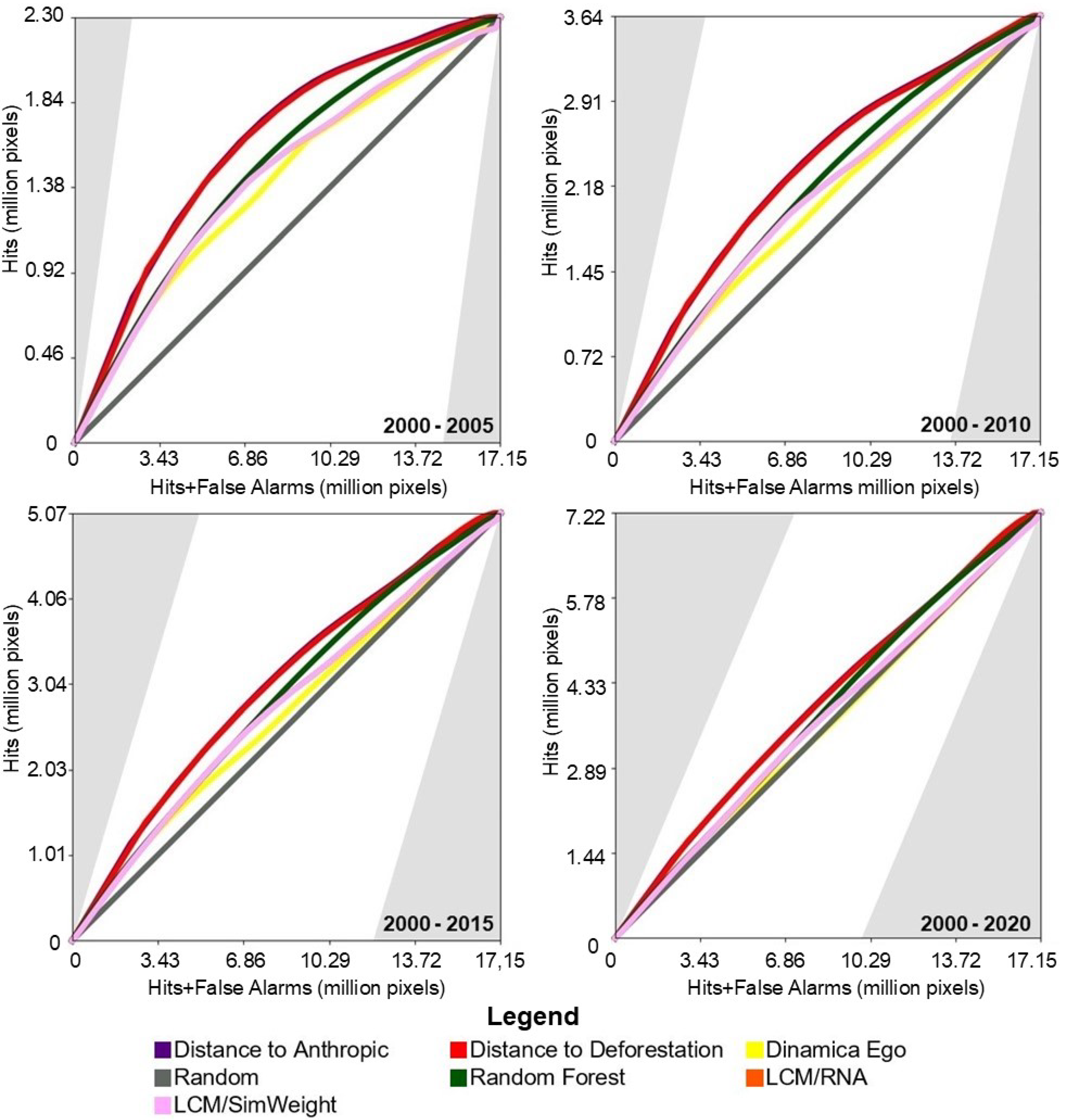
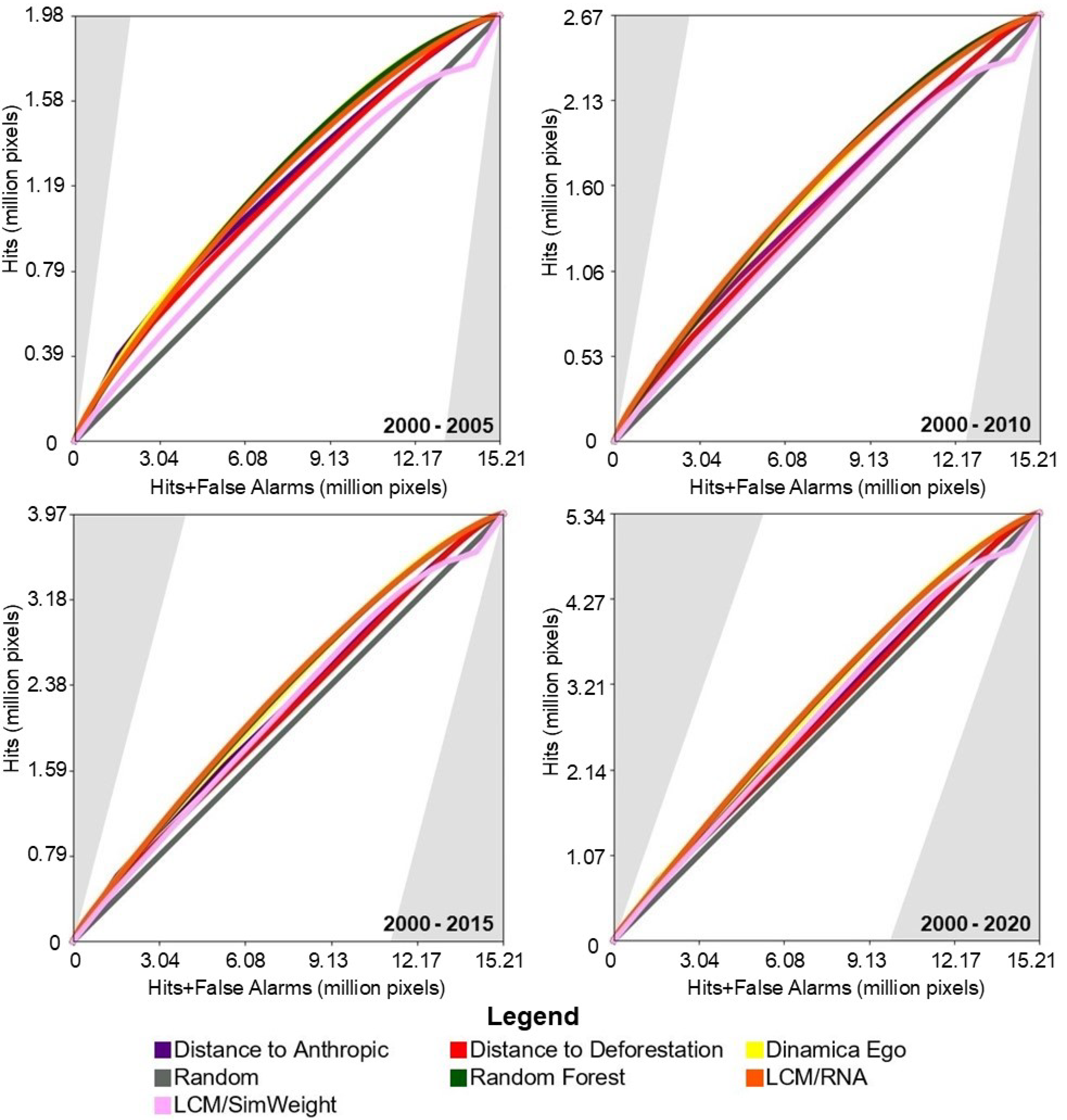
Figure 4 shows the results of the TOC evaluation. It can be observed that in all prediction periods, the performance of the baseline models was slightly superior to the machine-learning-based models.
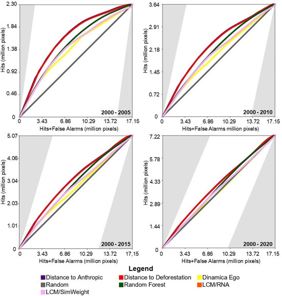
Figure 4.
TOC of the models for the study area in the Amazon biome.
For the study area in the Cerrado biome, Table 2 presents the AUC results found for the probability surfaces. The models with the best performance were Random Forest and ANN-TerrSet. The baseline models and Weights of Evidence–Dinamica Ego achieved slightly lower performance, while the model using Sim Weight—TerrSet obtained the worst performance.
Table 2.
AUC values of the models for the study area in the Cerrado biome.
Figure 5 presents the results of the TOC evaluation. For this study area, the baseline models achieved intermediate TOC values, outperforming two of the four machine-learning-based models.
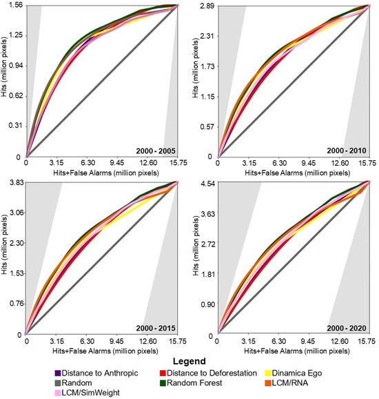
Figure 5.
TOC of the models for the study area in the Cerrado biome.
For the study area in the Pampa biome, the AUC results for the probability surfaces are presented in Table 3. Random Forest, Weights of Evidence–Dinamica Ego, and ANN–TerrSet methods presented better performance. The baseline model of distance to anthropogenic uses in 2000 showed a slightly lower AUC values. The models with the lowest values were the distance from vegetation suppression between 1995 and 2000 and Sim Weight—TerrSet.
Table 3.
AUC values of the models for the study area in the Pampa biome.
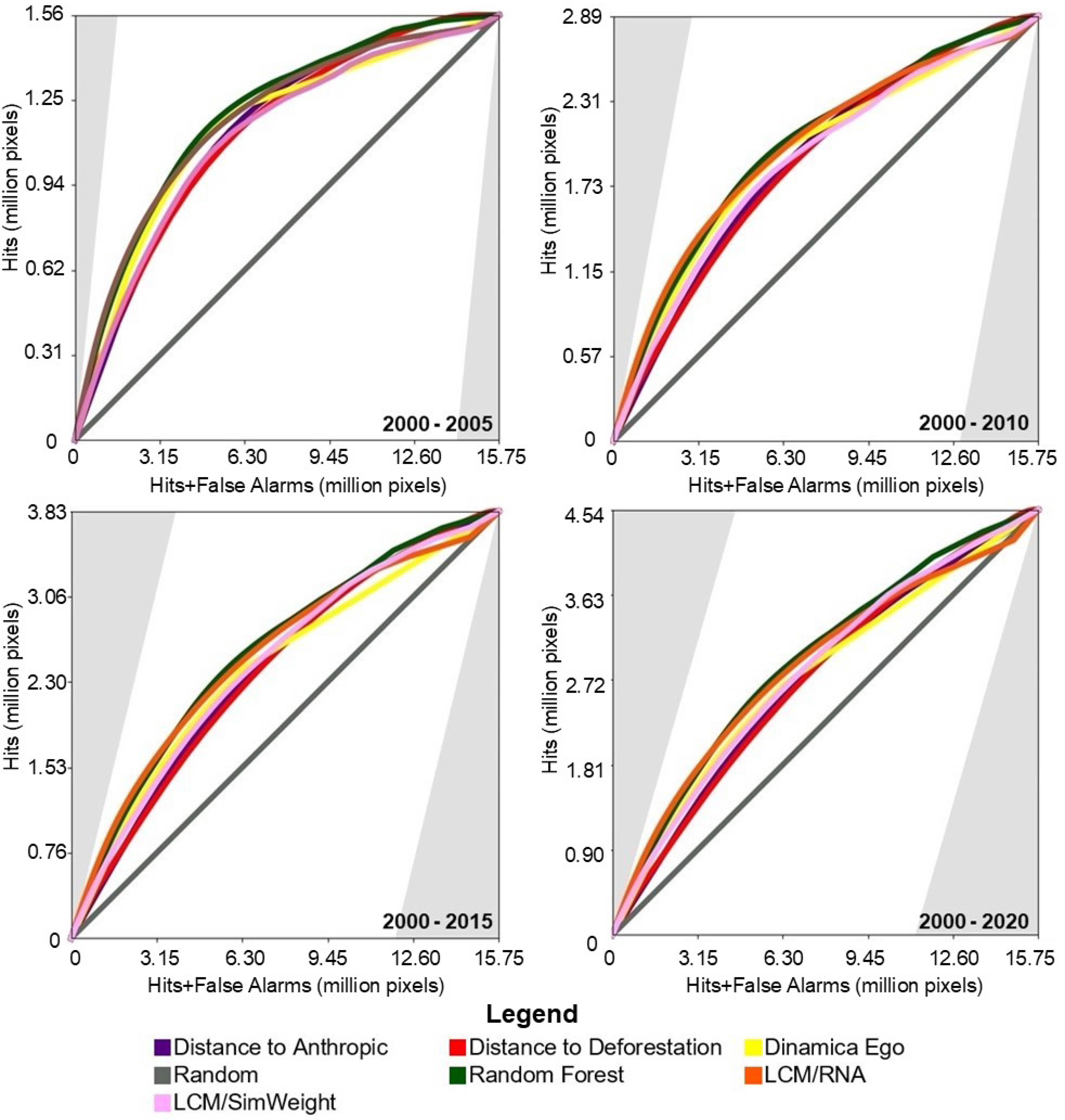
Figure 6 presents the results of the TOC evaluation. For this study area, with the exception of the Sim Weight—TerrSet model, machine learning models demonstrated superior performance compared to baseline models.

Figure 6.
TOC of the models for the study area in the Pampa biome.
In general, it is observed that for all study areas in each prediction period, the models performed similarly to each other. Nevertheless, it can be seen that the further away from the training period the prediction is made, the worse the model’s performance tends to be. This is observed in all tested conditions, regardless of the method or study area.
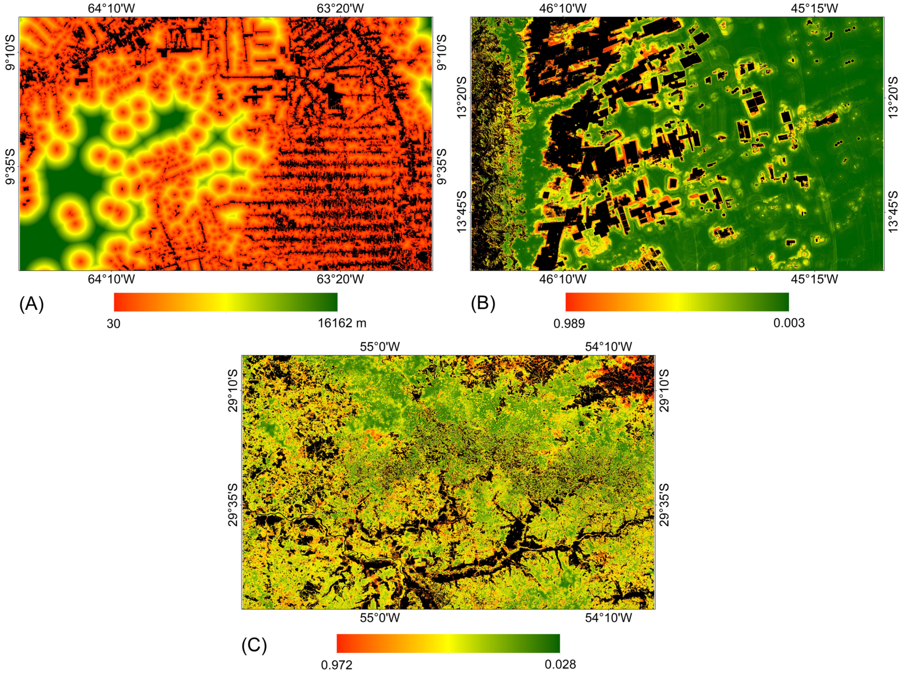
Figure 7 presents the probability surfaces with the highest average AUC values over the four prediction periods for each study area. For each model, the same probability surface was used to allocate changes in the four prediction periods. It is noted that for the study area in the Amazon biome, the areas considered most susceptible to vegetation suppression are located near the areas defined as anthropic uses in the year 2000. In contrast, for the study areas in the Pampa and Cerrado biomes, the areas considered most susceptible to vegetation suppression were defined by training with machine learning methods.
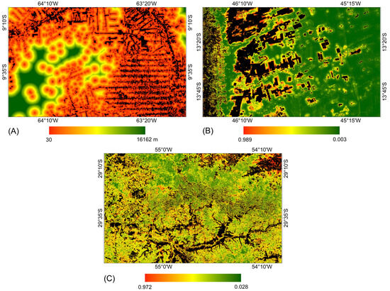
Figure 7.
Probability surface with the highest average AUC value over the prediction periods for each study area. (A) Amazon: distance from anthropic uses from 2000. (B) Cerrado: Random Forest. (C) Pampa: Random Forest.
3.2. Accuracy Assessment of the Predicted Maps
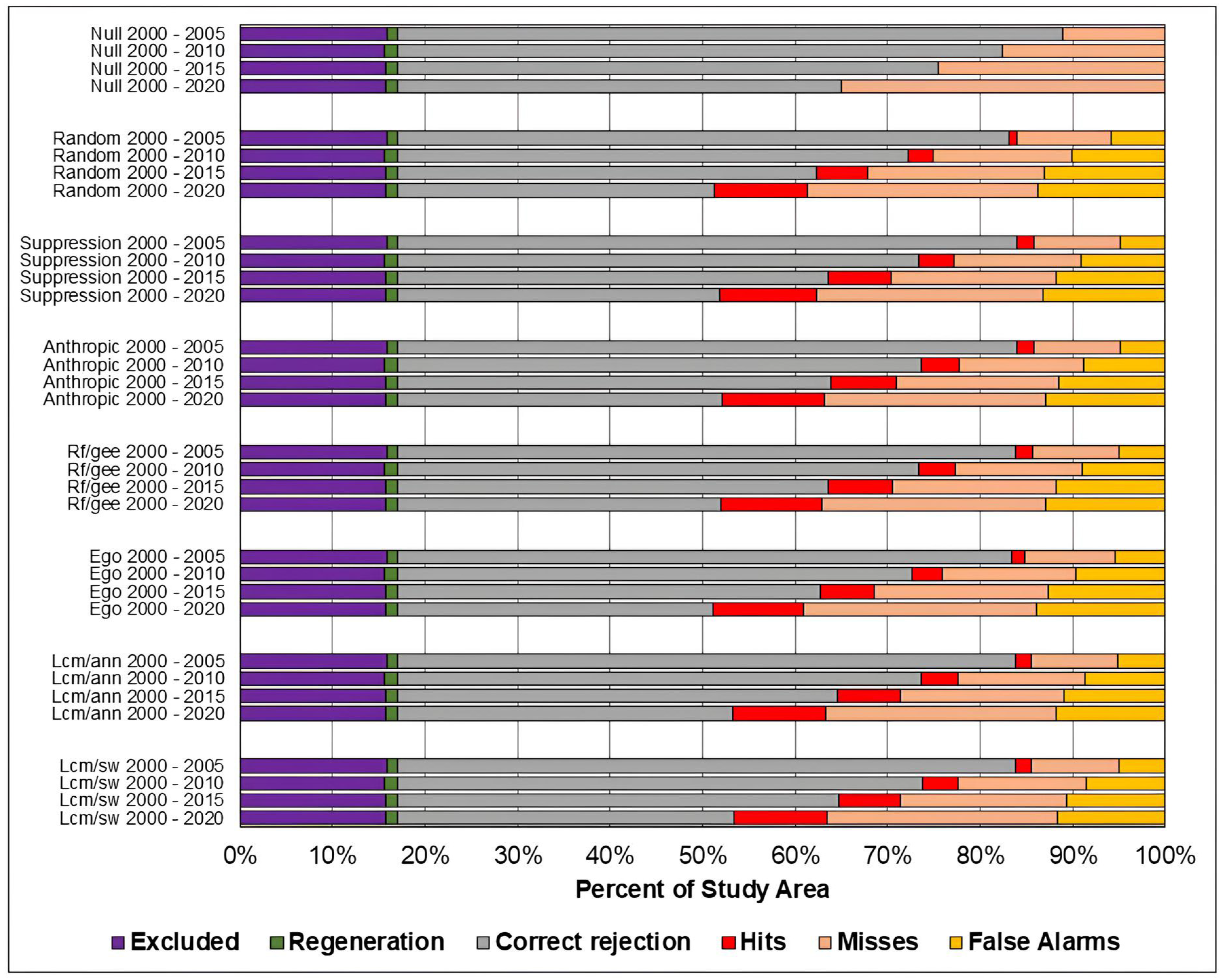
Figure 8, Figure 9 and Figure 10 present, respectively, for the study areas in the Amazon, Cerrado, and Pampa biomes, the results of the evaluation of predicted maps using the three-map technique. The components of excluded areas, shown in purple, and regeneration, shown in green, have the same size for each study area and prediction period, regardless of the model. For the null change model, misses, false alarms, and hits cannot be computed because there is no change to compare with the reference map.
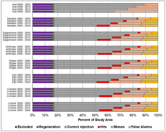
Figure 8.
Evaluation of the predicted maps for the study area in the Amazon biome using the three-map comparison method.
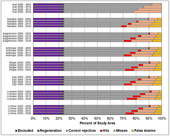
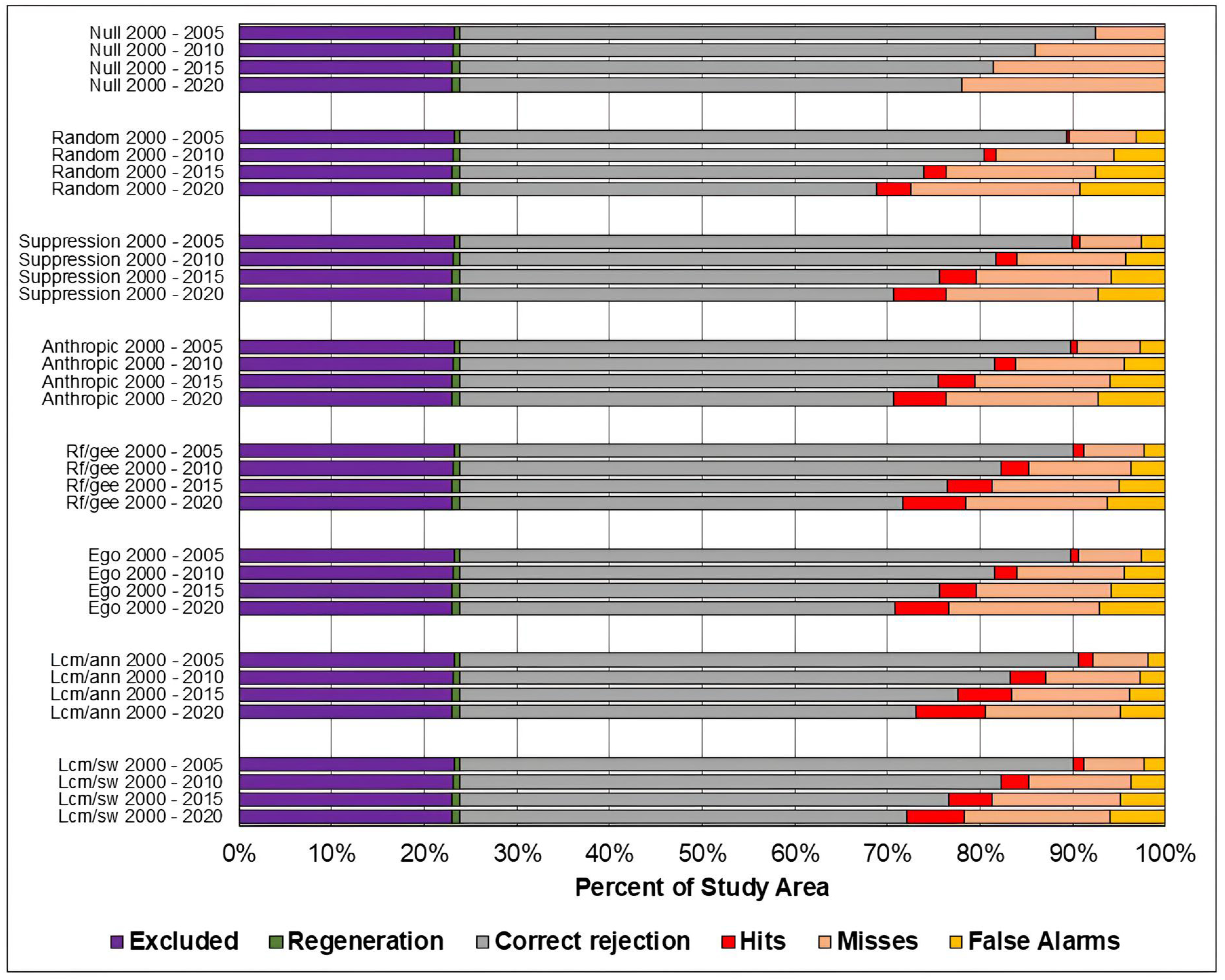
Figure 9.
Evaluation of the predicted maps for the study area in the Cerrado biome using the three-map comparison method.
As in the TOC assessment, the components of the three-map assessment were similar across models across all prediction periods, and worsened as the prediction period increased. Considering the Overall accuracy, the null change model outperformed the other in most cases, although with small differences. The exceptions occurred in the study area of the Cerrado biome for the predictions in the years 2010, 2015, and 2020. For 2010 and 2015, the ANN-TerrSet model outperformed the null change model. For 2020, the ANN-TerrSet, Sim Weight—TerrSet, and Random Forest models performed better than the null change model.
When comparing the results of baseline models with those of machine learning-based models, no clear distinction is observed between the two categories of models.
It can be observed that the quantity of misses was greater than false alarms for all study areas, models, and prediction periods. This indicates that disagreements due to the omission of changes contained in the reference were greater than disagreements due to the allocation of incorrectly predicted changes.
It is noted that the component of correct rejection is the most abundant in all scenarios, indicating that the main source of agreement was the prediction of persistence. Furthermore, when comparing the results of the Sim Weight and ANN methods with the other models, a larger area of correct rejections and fewer hits, omissions, and false alarms is observed. This occurs mainly because these models predict a smaller amount of changes when compared to the others.
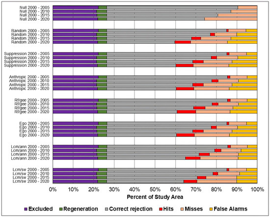
Figure 10.
Evaluation of the predicted maps for the study area in the Pampa biome using the three-map comparison method Table 4 presents the Figure of Merit values for all models and prediction periods in the study area of the Amazon biome. The models that achieved the highest Figure of Merit values for the prediction of 2005 were distance from anthropogenic uses and distance from vegetation suppression, while the models with the lowest values were random and Weights of Evidence–Dinamica Ego. For the 2010 and 2015 predictions, the highest values were found for the distance from anthropogenic uses and ANN-TerrSet models, while the lowest values were obtained for the Random and Dinamica EGO models. And for the 2020 prediction, the highest values were found for the distance from anthropogenic uses and Random Forest models, while the lowest values were found for the Random and Weights of Evidence–Dinamica Ego models.
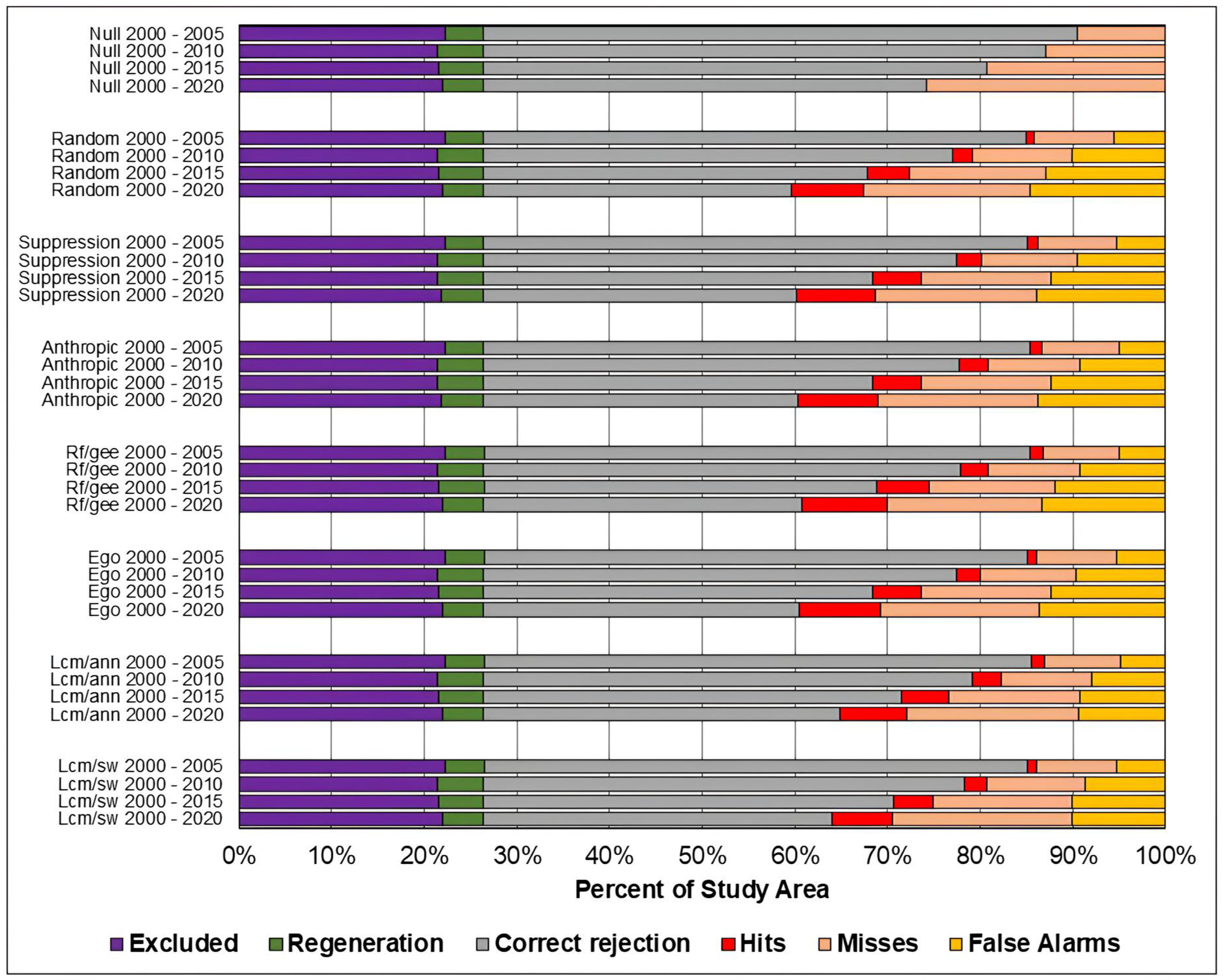
Table 4.
Figure of Merit for the models of the study area in the Amazon biome.
Table 4.
Figure of Merit for the models of the study area in the Amazon biome.
| Baseline Models | Machine-Learning-Based Models | ||||||
|---|---|---|---|---|---|---|---|
| Anthropic | Suppression | Random | ANN | Sim Weight | Random Forest | Dinamica Ego | |
| 2000–2005 | 0.114 | 0.114 | 0.053 | 0.104 | 0.103 | 0.107 | 0.079 |
| 2000–2010 | 0.155 | 0.143 | 0.098 | 0.148 | 0.147 | 0.146 | 0.117 |
| 2000–2015 | 0.195 | 0.184 | 0.146 | 0.191 | 0.189 | 0.187 | 0.157 |
| 2000–2020 | 0.228 | 0.219 | 0.205 | 0.216 | 0.214 | 0.225 | 0.201 |
Table 5 presents the Figure of Merit values for all models and prediction periods in the study area of the Cerrado biome. The models that obtained the highest Figure of Merit values for the 2005 prediction were ANN-TerrSet and distance from vegetation suppression, while the models with the lowest values were random and Weights of Evidence–Dinamica Ego. For the 2010 prediction, the highest values were found for the ANN-TerrSet and Sim Weight-TerrSet models, while the lowest values were for the Random and Weights of Evidence–Dinamica Ego models. And for the 2015 and 2020 predictions, the highest values were found for the ANN-TerrSet and Random Forest models, while the lowest values were for the Random and Weights of Evidence–Dinamica Ego models.
Table 5.
Figure of Merit for the models of the study area in the Cerrado biome.
Table 6 presents the Figure of Merit values for all models and prediction periods in the study area of the Pampa biome. The models that achieved the highest Figure of Merit values for the predictions of 2005, 2010, and 2015 were ANN-TerrSet and Random Forest, while the lowest values were the random and Sim Weight—TerrSet models. And for the 2020 prediction, the highest values were found for the Random Forest and Weights of Evidence–Dinamica Ego models, while the lowest values were for the Sim Weight-TerrSet and Random models.
Table 6.
Figure of Merit for the models of the study area in the Pampa biome.
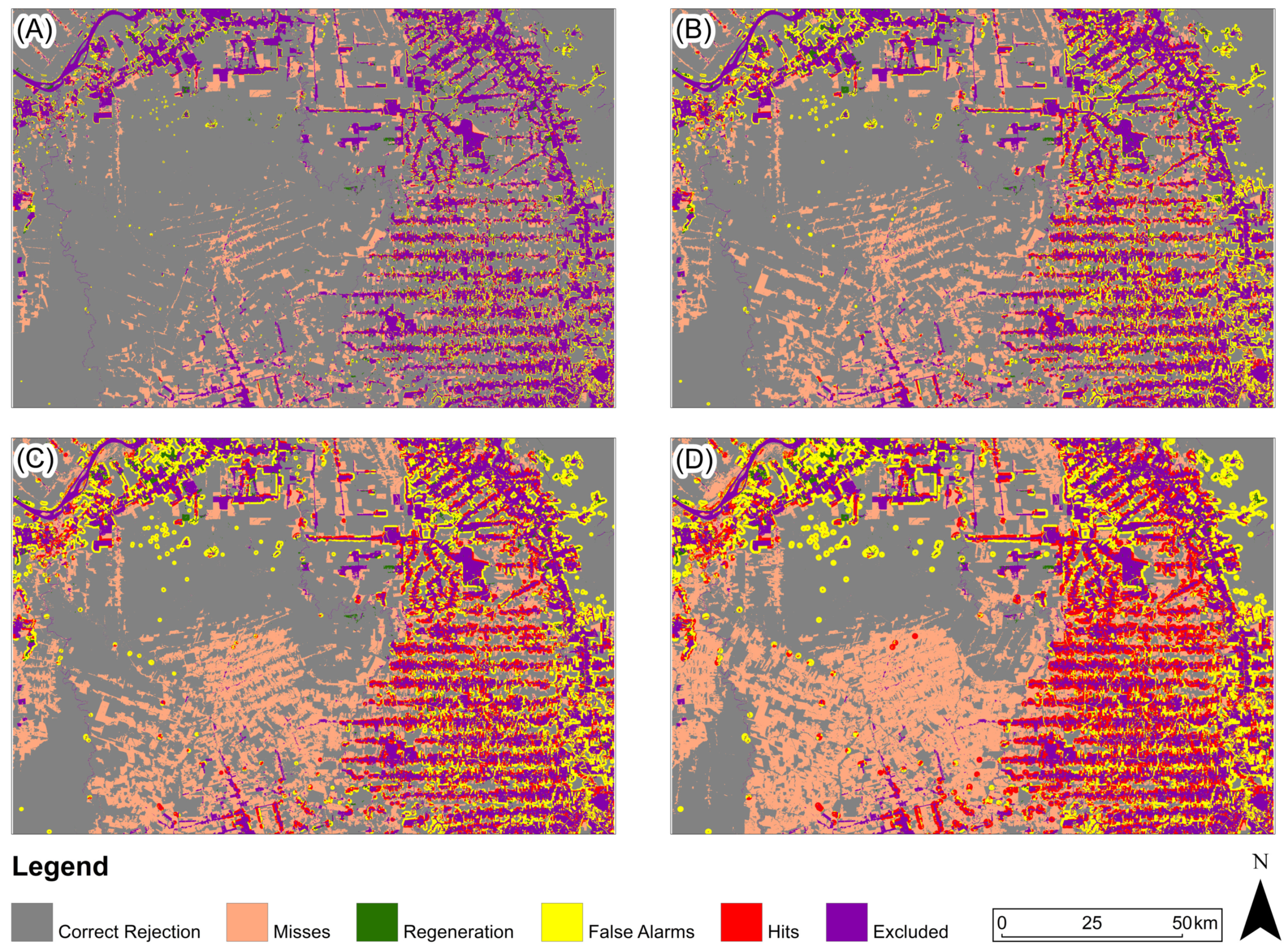
Figure 11, Figure 12 and Figure 13 present, for the three study areas, the predictive map that obtained the highest Figure of Merit value for each prediction period. For the study area in the Amazon biome (Figure 11), the predicted map with the highest Figure of Merit value for all prediction periods was generated based on the Euclidean distance from anthropogenic uses in 2000.
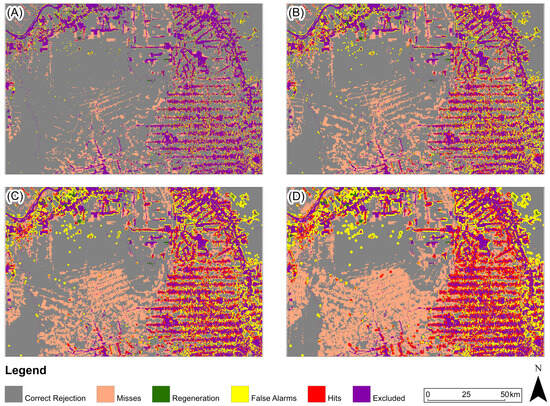
Figure 11.
Three-map evaluation: Amazon Biome: (A) 2005, (B) 2010, (C) 2015, (D) 2020. The model presented for all periods is based on Euclidean distance from anthropogenic in 2000.

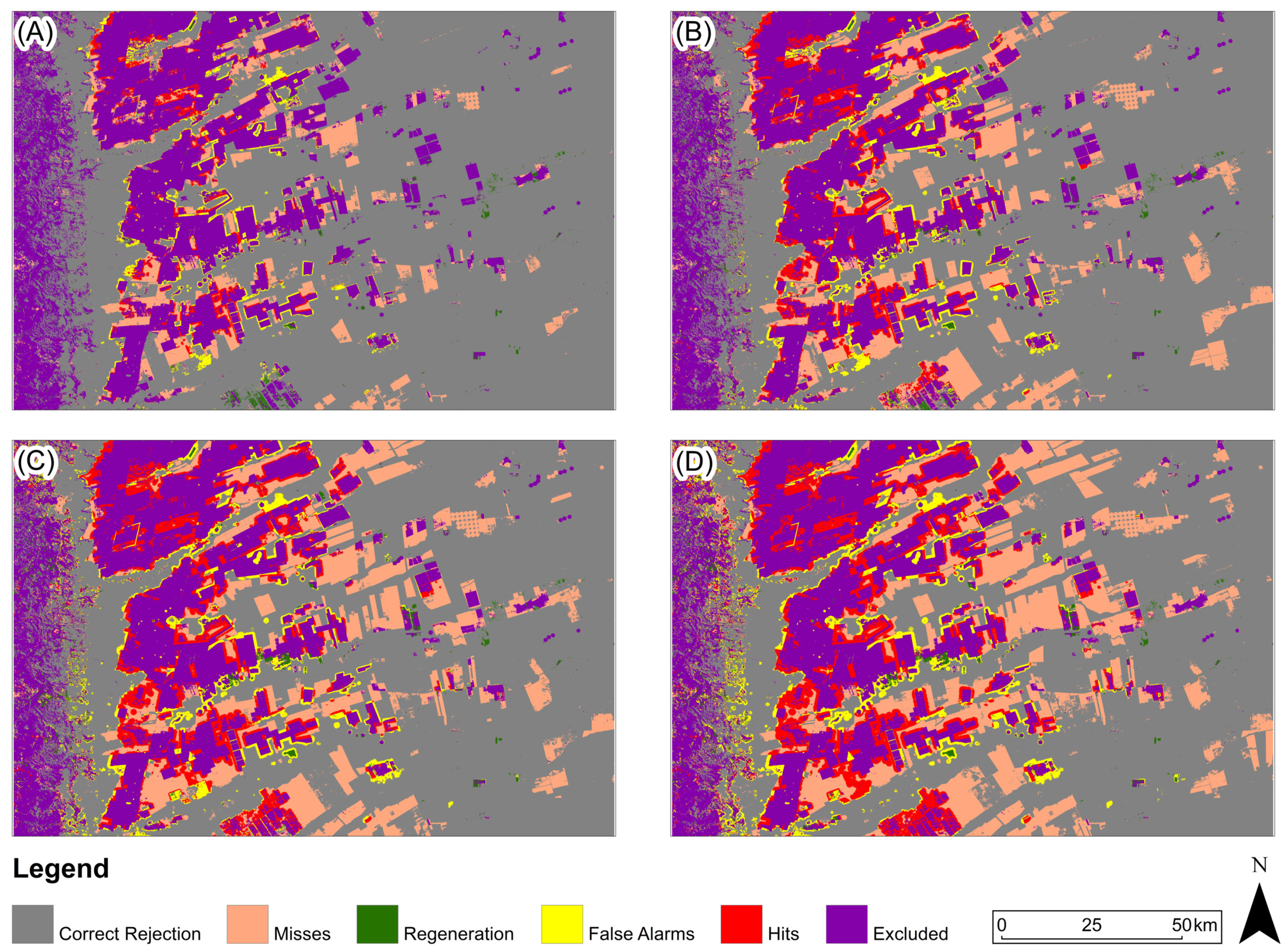
Figure 12.
Three-map evaluation: Cerrado Biome: (A) 2005, (B) 2010, (C) 2015, (D) 2020. The model presented for all periods is ANN-TerrSet.
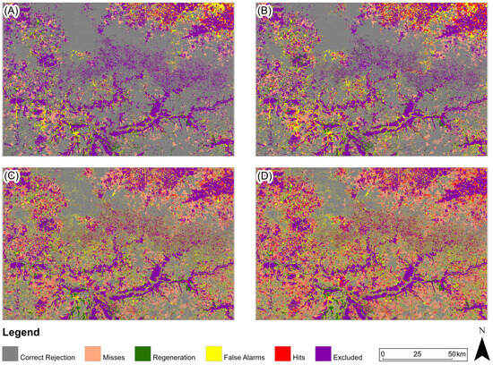
Figure 13.
Three-map evaluation: Pampa Biome: (A) 2005, (B) 2010, (C) 2015, (D) 2020. The model presented for 2005 and 2010 is ANN-TerrSet, and for 2015 and 2020, it is Random Forest.
For the study area in the Cerrado biome (Figure 12), predicted map with the highest Figure of Merit value for all periods was generated based on the ANN-TerrSet model.
For the study area in the Pampa biome (Figure 13), the predicted map with the highest Figure of Merit value for 2005 and 2010 was generated based on the ANN-TerrSet model, and for the years 2015 and 2020 based on the Random Forest model.
4. Discussion
The results presented in this article provide an opportunity to discuss relevant topics regarding land-use change models. We focus on three main topics: the importance of using rigorous methods in assessing the accuracy of model results, the sources of disagreement in modeling, and the comparison between baseline models and machine-learning-based models.
4.1. The Importance of Using Rigorous Methods in Assessing the Accuracy of Model Results
Accuracy assessment is a crucial step in land-use change modeling, enabling users to understand strengths and weaknesses of each method. Unfortunately, the land-use change modeling community tends to underestimate the importance of accuracy assessment. Many studies do not perform any type of accuracy assessment, while others frequently use flawed or potentially misleading methods. The ROC and overall accuracy stand out as the accuracy metrics most commonly employed [1,2].
The Area Under the Curve (AUC) of ROC is used in many studies as the sole approach for evaluating the accuracy of probability surfaces. Examples can be found in Park et al. (2010) [24], Liao; Wei (2014) [25], Kucsicsa et al. (2019) [26], Voight et al. (2019) [27], and Colman et al. (2024) [28]. This practice is problematic because the ROC is generally used to evaluate the probability surface relative to the change data observed during the training period. Thus, it only serves to indicate the fit of the training, not providing information about the ability of the probability surface to differentiate changes and no changes in the prediction periods. Another common practice is to provide only the AUC value without presenting the shape of the curve. This can be misleading because different curve shapes can have the same AUC value. Pontius and Parmentier (2014) [6] comment on the shape of the curve: “The lower left indicates the association between the high ranking index values and the Boolean feature, while the upper right indicates the association between the low ranking index values and the Boolean feature”. Therefore, analyzing the shape of the curve allows for a better understanding of the model’s performance. For predicted maps investigating rare changes, the lower left corner should be analyzed in particular.
Additionally, ROC does not provide any information about the spatial accuracy of change allocation. The results presented in this work show that the highest AUC value does not always coincide with the best predicted map. In the study area of the Cerrado biome, for example, the Random Forest model obtained the highest AUC values for all periods. However, when evaluating the predicted maps by Figure of Merit, the ANN-TerrSet model showed the best performance. This demonstrates the importance of evaluating both the probability surface and the prediction map.
Overall accuracy is a metric used to estimate the percentage of pixels correctly allocated on the prediction map. In several studies, this is the only approach used to evaluate the predicted map. Examples can be found in Park et al. (2010) [24], Lin et al. (2011) [8], Ballestores Junior; Qiu. (2012) [29], Cushman et al. (2017) [30], Kucsicsa et al. (2019) [26]. Overall accuracy can be potentially misleading because it often considers the correct rejection component and excluded areas as model successes. However, the primary goal of developing a land-use change model is to predict future changes. Therefore, a rigorous evaluation method should analyze the hits, misses, and false alarms components. This issue can be illustrated by the predicted map derived from the Euclidean distance model from anthropogenic uses in the Amazon biome study area in 2005. The overall accuracy of the map was 85.6%, of which 96.6% is composed of correct rejections and excluded areas. When analyzing the hits, we observe that it was approximately seven times smaller than the sum of the misses and false alarms. Thus, analyzing only global accuracy gives a misleading impression of the prediction’s ability to represent future land-use changes.
For the accuracy assessment of the probability surface, it has been demonstrated that the TOC provides more information compared to the ROC. Another good practice is the use of baseline models. The results of this work demonstrate that baseline models are more rigorous comparison methods than randomization, aiding in the interpretation of the performance of machine-learning-based models [7,9,11,23].
For the evaluation of predicted maps, among the pixel-based methods, the three-map comparison and Figure of Merit approaches provide measures that allow understanding the size and proportion of agreement and disagreement components. This enables a detailed evaluation of the model’s performance in capturing the components related to changes [3,12].
Additionally, comparing the maps with a null change model is another recommended practice [3,31]. It is expected that a prediction model should produce more accurate results than a null change model, but this is not always true. The results of this work demonstrate that, in most situations, the maps predicted with several models presented performance inferior to the use of a null change model.
Another approach used in this study was the comparison with random-based models. Although the latter generally performed worse, the size of their agreement and disagreement components presented the same pattern as the other models. It was evident that the majority of the agreements (hits and correct rejections) across all models are due to chance. This is an important consideration, as the agreement component are often mistakenly attributed to the good performance of the models.
Based on these results, it is clear that some common practices for evaluating models are flawed. In order to maximize the usefulness of predictions, it is necessary to understand their disagreements in detail. Although the models do not perfectly represent reality, some of them can be useful for specific objectives.
4.2. Sources of Disagreement in Land-Use Change Modeling
The disagreements observed in the results the prediction models originate from different sources. Among the possible origins, we can highlight land-use maps, the amount of expected changes for the future, predictive variables, and the identification of patterns of change.
Land-use maps are utilized in various stages of modeling, including the identification of changes during training, the preparationof predictive variables, and the accuracy assessment itself. Regardless of the method used to classify land use, the resulting maps do not represent the space perfectly [10,13,32,33]. For the case of the MapBiomas project, the overall accuracy of the products is 96.8% for the Amazon biome, 84.7% for the Cerrado biome, and 85.8% for the Pampa biome [34]. This shows that the use of land-use maps adds confusion to the models, which is an inherent limitation of any modeling process. Knowing this difficulty, it is important that land-use maps with known accuracy are used in modeling, which makes it possible to identify the uncertainties that the use of these products introduces into the models.
The predicted amount of change is another point of difficulty. When defining the expected amount of future changes based on the context of the present and past, there is no guarantee that the transition rates will remain the same [35]. The results found for the study area of the Cerrado Biome are good examples of this issue. The amount of vegetation suppression found for the training period (1995–2000) corresponds to 3.59% of the total study area. This rate was assumed to define the expected amount of change for the future. However, from 2000 to 2005, the amount of vegetation suppression corresponds to 7.58% of the total area. For 2005 to 2010, this percentage was 7.05%. Between 2010 and 2015, it was 5.25%. And from 2015 to 2020, it was 4.03%. In this sense, it is clear that the amount of vegetation suppression that occurred during the training period was less than in all the prediction periods. As a result, the predictions of vegetation suppression for the Cerrado biome study area predicted fewer changes than actually occurred. This resulted in a large number of misses, surpassing the number of false alarms in all situations. For this problem, regardless of the strategy employed, there are no guarantees of better results.
The spatial variables used to identify the patterns that explain land-use changes may have various errors. In addition to the variables derived from land-use maps, it is common to use Euclidean distance surfaces from elements such as highways, conservation units, protected areas, etc. If these elements have errors in location, delineation, georeferencing, or others, their use adds confusion to the modeling process. Therefore, this stage deserves special attention, as it is necessary to evaluate whether the products used to develop the predictive variables appropriatelyrepresent what is desired.
Furthermore, identifying patterns of land-use change during the training period does not guarantee that these patterns will remain the same during the prediction stage. Between the training and prediction periods, political, economic, social, and infrastructural changes may occur, driving the occupation of areas not identified in the training as susceptible to change. Additionally, when modeling changes for large areas, different locations may have different factors that induce the occurrence of changes [36].
Our results show that, for all models and study areas, the further away from the training period, the worse the models perform. Knowing these limitations, the models should be interpreted considering that the patterns of change may shift. Additionally, knowing the spatial variability of the factors that explain the changes, the definition of the extrapolation area of the patterns identified in the training should be carried out with caution.
4.3. Comparison Between Machine-Learning-Based and Baseline Models
For the predictions presented in the results, it is observed that the models of both natures obtained similar performances in all the evaluation methods. Shafizadeh-Moghadam et al. (2021) [7] and Harati et al. (2021) [9] verified the same when comparing baseline and machine-learning-based models for predicting urban sprawl and forest insect disturbance.
Possible reasons for similar performance can be as follows: (1) The amount of change during the training period was significantly different from the prediction period. Therefore, a large amount of change was likely allocated to areas not considered susceptible by the machine-learning-based models. (2) For the Amazon and Cerrado study areas, a significant shift in the spatial patterns of change was observed between the training and prediction periods. Consequently, a significant portion of the change was allocated to areas that were not predicted to be susceptible according to the machine-learning-based models. (3) It is known that change processes are influenced by their surroundings [4]. The vegetation suppression investigated was likely related to proximity to anthropogenic uses or to past suppressions. And (4) predicting natural vegetation suppression is challenging. A variety of factors, including political changes, economic conditions, environmental regulations, personal motivations, mineral discoveries, and wars, can influence the quantity and location of suppressions. Given the complexity of the problem, it is expected that all models will produce a significant number of false alarms and omissions. This is supported by the observation that the random model performed on par with the others in all scenarios.
The results show that the effort invested in developing machine-learning-based models did not provide accuracy better than baseline models. Furthermore, it is observed that, in baseline models, there is a direct relationship between the prediction of vegetation suppression and the proximity to the class of anthropogenic uses and past vegetation suppressions. For machine-learning-based models, it is not explicitly clear which criteria were used to define probability to vegetation suppression. In view of this, the use of baseline models may be advantageous due to their ease of formulation, understanding, and similar performance to machine-learning-based models. If machine-learning-based models are used, the baseline models can be used to compare the results.
5. Conclusions
The results and discussions presented in this work highlight important points about land-use change modeling: (1) The use of baseline land-use change models should be considered due to their quick and easy formulation process, requiring few data and not needing powerful hardware; their results are easily interpretable; and their performance can be comparable to methods based on machine learning. (2) Land-use change models have a limited ability to predict future scenarios. All the land-use change models applied in this work, regardless of the formulation method, obtained more disagreements than correctly predicted changes. Additionally, analyzing the performance of randomness-based models shows that a considerable portion of the hits of all models is due to chance. (3) Predicting land-use change for periods far from training tends to generate less accurate results than for closer periods. (4) The evaluation of model results using inappropriate methods leads to an interpretation that generally overestimates the accuracy of predictions. It was evident that the exclusive use of evaluation methods such as the ROC and overall accuracy generated misleading results.
To enhance the accuracy of future models, the following recommendations could be considered: (1) Regarding the selection of predictive variables, the relevance could be tested and quantity increased. (2) The allocation of changes could be improved by considering exogenous variables (such as agricultural frontier expansion) and change constraints (such as protected lands or areas with high slopes). And (3) non-constant transition rates could be tested.
Given the increasing use of land-use change models in a wide variety of applications, it is important for the scientific community to recognize the limitations of this technique to better employ it. So, it is recommended that researchers consider indications as the presented in this document to better understand and communicate the results of this type of model.
Supplementary Materials
The computational codes, the reclassification of land-use maps, the spatial variables, the probability models for vegetation suppression, and predicted maps used in this article can be accessed through the link: https://github.com/macleidivarnier/Evaluating-the-Accuracy-of-Land-Use-Change-Models-for-Predicting-Vegetation-Loss-Across-Brazilian-B (accessed on 2 February 2025).
Author Contributions
Conceptualization, M.V. and E.J.W.; methodology, M.V. and E.J.W.; software, M.V.; validation, M.V.; formal analysis, M.V.; investigation, M.V.; resources, M.V.; data curation, M.V.; writing—original draft preparation, M.V.; writing—review and editing, M.V. and E.J.W.; visualization, M.V.; supervision, E.J.W. All authors have read and agreed to the published version of the manuscript.
Funding
This research was funded by the Coordination of Improvement of Higher Education Personnel of Brazil (CAPES), grant number 8887.721596/2022-00.
Data Availability Statement
The data presented in this study are available upon request from the corresponding author.
Acknowledgments
This work was supported by the Brazilian Coordination for the Improvement of Higher Education Personnel (CAPES) through a master’s scholarship for the corresponding author, which is gratefully acknowledged.
Conflicts of Interest
The authors declare no conflicts of interest.
Abbreviations
The following abbreviations are used in this manuscript:
| ANN | Artificial Neural Network |
| AUC | Area Under the Curve |
| ASTER | Advanced Spaceborne Thermal Emission and Reflection Radiometer |
| GLAS | Geoscience Laser Altimeter System |
| GEE | Google Earth Engine |
| IBGE | Brazilian Institute of Geography and Statistics |
| ICESat | Ice, Cloud, and Land Elevation Satellite |
| MLP | Multi-Layer Perceptron |
| ROC | Receiver Operating Characteristic Curve |
| SRTM | Shuttle Radar Topographic Mission |
| TOC | Total Operating Characteristic Curve |
References
- Van Vliet, J.; Bregt, A.K.; Brown, D.G.; van Delden, H.; Heckbert, S.; Verburg, P.H. A review of current calibration and validation practices in land-change modeling. Environ. Model. Softw. 2016, 82, 174–182. [Google Scholar] [CrossRef]
- Aburas, M.M.; Ahamad, M.S.S.; Omar, N.Q. Spatio-temporal simulation and prediction of land-use change using conventional and machine learning models: A review. Environ. Monit. Assess. 2019, 191, 191–205. [Google Scholar] [CrossRef] [PubMed]
- Pontius, R.G.; Boersma, W.; Castella, J.; Clarke, K.; NIJS, T.; Dietzel, C.; Duan, Z.; Fotsing, E.; Goldstein, N.; Kok, K. Comparing the input, output, and validation maps for several models of land change. Ann. Reg. Sci. 2007, 42, 11–37. [Google Scholar] [CrossRef]
- Soares-Filho, B.S.; Cerqueira, G.C.; Pennachin, C.L. Dinamica—A stochastic cellular automata model designed to simulate the landscape dynamics in an Amazonian colonization frontier. Ecol. Model. 2002, 154, 217–235. [Google Scholar] [CrossRef]
- Sangermano, F.; Eastman, J.R.; Zhu, H. Similarity Weighted Instance-based Learning for the Generation of Transition Potentials in Land Use Change Modeling. Trans. Gis 2010, 14, 569–580. [Google Scholar] [CrossRef]
- Pontius, R.G.; Parmentier, B. Recommendations for using the relative operating characteristic (ROC). Landsc. Ecol. 2014, 29, 367–382. [Google Scholar] [CrossRef]
- Shafizadeh-Moghadam, H.; Minaei, M.; Pontius, R.G.; Asghari, A.; Dadashpoor, H. Integrating a Forward Feature Selection algorithm, Random Forest, and Cellular Automata to extrapolate urban growth in the Tehran-Karaj Region of Iran. Comput. Environ. Urban Syst. 2021, 87, 101595. [Google Scholar] [CrossRef]
- Lin, Y.; Chu, H.; Wu, C.; Verburg, P.H. Predictive ability of logistic regression, auto-logistic regression and neural network models in empirical land-use change modeling—A case study. Int. J. Geogr. Inf. Sci. 2011, 25, 65–87. [Google Scholar] [CrossRef]
- Harati, S.; Perez, L.; Molowny-Horas, R.; Pontius, R.G. Validating models of one-way land change: An example case of forest insect disturbance. Landsc. Ecol. 2021, 36, 2919–2935. [Google Scholar] [CrossRef]
- Pontius, R.G.; Millones, M. Death to Kappa: Birth of quantity disagreement and allocation disagreement for accuracy assessment. Int. J. Remote Sens. 2011, 32, 4407–4429. [Google Scholar] [CrossRef]
- Pontius, R.G.; Si, K. The total operating characteristic to measure diagnostic ability for multiple thresholds. Int. J. Geogr. Inf. Sci. 2014, 28, 570–583. [Google Scholar] [CrossRef]
- Pontius, R. Criteria to Confirm Models that Simulate Deforestation and Carbon Disturbance. Land 2018, 7, 105. [Google Scholar] [CrossRef]
- Foody, G. Explaining the unsuitability of the kappa coefficient in the assessment and comparison of the accuracy of thematic maps obtained by image classification. Remote Sens. Environ. 2020, 239, 111630. [Google Scholar] [CrossRef]
- Souza, C.M.; Shimbo, J.Z.; Rosa, M.R.; Parente, L.L.; Alencar, A.; Rudorff, B.F.; Hasenack, H.; Matsumoto, M.; Ferreira, L.G.; E Souza-Filho, P.W.; et al. Reconstructing Three Decades of Land Use and Land Cover Changes in Brazilian Biomes with Landsat Archive and Earth Engine. Remote Sens. 2020, 12, 2735. [Google Scholar] [CrossRef]
- Pontius, R.G.; Bilintoh, T.; Oliveira, G.; Shimbo, J. Trajectories of losses and gains of soybean cultivation during multiple time intervals in western Bahia, Brazil. Proc. Space Week Nordeste 2023, 1–4. Available online: https://proceedings.science/swn-2023/trabalhos/trajectories-of-losses-and-gains-of-soybean-cultivation-during-multiple-time-int?lang=pt-br (accessed on 10 January 2025).
- Mapbiomas: O Projeto. Available online: https://mapbiomas.org/o-projeto (accessed on 25 June 2023).
- Nasadem: Creating a New NASA Digital Elevation Model and Associated Products. Available online: https://www.earthdata.nasa.gov/esds/competitive-programs/measures/nasadem (accessed on 17 September 2023).
- Instituto Brasileiro de Geografia E Estatística: Bases Cartográficas Contínuas (Versão 2021). Available online: https://geoftp.ibge.gov.br/cartas_e_mapas/bases_cartograficas_continuas/bc250/ (accessed on 7 May 2023).
- Gorelick, N.; Hancher, M.; Dixon, M.; Ilyushchenko, S.; Thau, D.; Moore, R. Google Earth Engine: Planetary-scale geospatial analysis for everyone. Remote Sens. Environ. 2017, 202, 18–27. [Google Scholar] [CrossRef]
- Breiman, L. Random Forests. Mach. Learn. 2001, 45, 5–32. [Google Scholar] [CrossRef]
- Google: Machine Learning Glossary. Available online: https://developers.google.com/machine-learning/glossary (accessed on 17 May 2024).
- Google Earth Engine: Smile Random Forest. Available online: https://developers.google.com/earth-engine/apidocs/ee-classifier-smilerandomforest (accessed on 17 May 2024).
- Liu, Z.; Pontius, R.G. The Total Operating Characteristic from Stratified Random Sampling with an Application to Flood Mapping. Remote Sens. 2021, 13, 3922. [Google Scholar] [CrossRef]
- Park, S.; Jeon, S.; Kim, S.; Choi, C. Prediction and comparison of urban growth by land suitability index mapping using GIS and RS in South Korea. Landsc. Urban Plan. 2011, 99, 104–114. [Google Scholar] [CrossRef]
- Liao, F.; Wei, D. Modeling determinants of urban growth in Dongguan, China: A spatial logistic approach. Stoch. Environ. Res. Risk Assess. 2012, 28, 801–816. [Google Scholar] [CrossRef]
- Kucsicsa, G.; Popovici, E.; Bălteanu, D.; Dumitraşcu, M.; Grigorescu, I.; Mitrică, B. Assessing the Potential Future Forest-Cover Change in Romania, Predicted Using a Scenario-Based Modelling. Environ. Model. Assess. 2019, 25, 471–491. [Google Scholar] [CrossRef]
- Voight, C.; Hernandez-Aguilar, K.; Garcia, C.; Gutierrez, S. Predictive Modeling of Future Forest Cover Change Patterns in Southern Belize. Remote Sens. 2019, 11, 823. [Google Scholar] [CrossRef]
- Colman, C.B.; Guerra, A.; Almagro, A.; Roque, F.O.; Rosa, I.M.D.; Fernandes, G.W.; Oliveira, P.T. Modeling the Brazilian Cerrado land use change highlights the need to account for private property sizes for biodiversity conservation. Sci. Rep. 2024, 14, 4559. [Google Scholar] [CrossRef] [PubMed]
- Ballestores Junior, F.; Qiu, Z. An integrated parcel-based land use change model using cellular automata and decision tree. Proc. Int. Acad. Ecol. Environ. Sci. 2012, 2, 53–69. [Google Scholar]
- Cushman, S.; Macdonald, E.; Landguth, E.; Malhi, Y.; Macdonald, D. Multiple-scale prediction of forest loss risk across Borneo. Landsc. Ecol. 2017, 32, 1581–1598. [Google Scholar] [CrossRef]
- Pontius, R.G.; Huffaker, D.; Denman, K. Useful techniques of validation for spatially explicit land-change models. Ecol. Model. 2004, 179, 445–461. [Google Scholar] [CrossRef]
- Congalton, R. A review of assessing the accuracy of classifications of remotely sensed data. Remote Sens. Environ. 1991, 37, 35–46. [Google Scholar] [CrossRef]
- Foody, G. Status of land cover classification accuracy assessment. Remote Sens. Environ. 2002, 80, 185–201. [Google Scholar] [CrossRef]
- Mapbiomas: Análise de Acurácia. 2024. Available online: https://brasil.mapbiomas.org/analise-de-acuracia/ (accessed on 28 April 2024).
- Pontius, R.G.; SPENCER, J. Uncertainty in Extrapolations of Predictive Land-Change Models. Environ. Plan. B Plan. Des. 2005, 32, 211–230. [Google Scholar] [CrossRef]
- Trigueiro, W.R.; Nabout, J.C.; Tessarolo, G. Uncovering the spatial variability of recent deforestation drivers in the Brazilian Cerrado. J. Environ. Manag. 2020, 275, 111243. [Google Scholar] [CrossRef]

Disclaimer/Publisher’s Note: The statements, opinions and data contained in all publications are solely those of the individual author(s) and contributor(s) and not of MDPI and/or the editor(s). MDPI and/or the editor(s) disclaim responsibility for any injury to people or property resulting from any ideas, methods, instructions or products referred to in the content. |
© 2025 by the authors. Licensee MDPI, Basel, Switzerland. This article is an open access article distributed under the terms and conditions of the Creative Commons Attribution (CC BY) license (https://creativecommons.org/licenses/by/4.0/).