Abstract
Understanding the changes in ecosystem quality caused by land use changes is critical for sustainable urban development and environmental management. This study investigates the spatial-temporal evolution of ecosystem quality in Wuhan from 2000 to 2020 and forecasts future trends under multiple land use scenarios for 2030. Using a “foundation-function-structure” assessment framework, we integrate system dynamics (SD), the Patch-generating Land Use Simulation (PLUS) model, and a neural network-based ecosystem quality inversion model to analyze land use transitions and their ecological impacts. The results indicate that rapid urban expansion has significantly contributed to the decline of cropland and forest areas, while impervious surfaces have increased, leading to notable ecological degradation. Simulations for 2030 under three scenarios—ecological protection, natural development, and economic priority—demonstrate that the ecological protection scenario yields the highest ecosystem quality, preserving landscape connectivity and mitigating degradation risks. In contrast, the economic priority scenario results in extensive urban expansion, exacerbating ecological stress. Under the ecological protection scenario from 2020 to 2023, the decline in ecosystem quality was primarily due to the expansion of urban fringes and the erosion of forest and grassland areas. The increase in ecosystem quality was mainly attributed to the transformation of early urban edge conflict zones into stable urban edge interior areas and the integration of fragmented ecological land patches. These findings highlight the need for strategic land use planning to balance economic growth and environmental conservation. This study provides a robust methodological framework for assessing and predicting ecosystem quality changes, offering valuable insights for policymakers and urban planners striving for sustainable development.
1. Introduction
Understanding the complex interplay between land use changes and ecosystem quality is crucial for sustainable regional development. Ecosystem quality, a multi-dimensional concept incorporating ecological elements, ecological function, and structural integrity, is vital for maintaining environmental resilience. However, anthropogenic activities, especially land use alterations [1,2], have significantly impacted ecosystem stability in many regions, and introduced challenges that necessitate comprehensive assessment frameworks.
Ecosystem quality assessment has evolved through various methodological advancements, including remote sensing ecological indices [3], landscape ecological quality [4], ecological risk [5], ecological security [6], ecosystem services [7,8] and ecosystem health [9]. Traditional approaches rely on single-type indicators such as remote sensing or landscape structure, or assess and express ecosystem quality in terms of a single dimension such as risk, security, services, or health. The increasing availability of high-resolution spatial data has facilitated multi-temporal ecosystem monitoring, allowing for more nuanced insights into degradation patterns and recovery processes [3,4]. The application of methods such as deep learning has further enhanced the assessment capabilities [9]. In addition, based on the analysis of historical changes in ecosystem quality, it is necessary to predict the future changes. Existing related studies, including future predictions of habitat quality [10], the remote sensing ecological index [11], and ecological risk [12,13], are mostly based on land use simulation, and they predict future changes in ecosystem quality in terms of a single dimension. The existing ecosystem quality assessment system and its multi-scenario simulation methods still need to be perfected, and it is difficult to better analyze and anticipate ecosystem responses to various land use strategies and climate projections.
Land use changes, including urban expansion, agricultural intensification, and afforestation, have been recognized as primary drivers of ecosystem quality fluctuations. Song [2] demonstrated that global land transformations significantly alter ecosystem service provision, while Kong [1] highlighted the spatial heterogeneity in ecological responses to land conversion. Rapid urbanization has led to the loss of wetlands and agricultural land, reducing habitat connectivity and increasing ecological stress. Additionally, land abandonment and reforestation have been identified as crucial processes influencing biodiversity and ecosystem stability [4].
Studies utilizing dynamic land use models, such as system dynamics (SD) [14] and Patch-generating Land Use Simulation (PLUS) [15], have shown that land transformation influences ecosystem quality by modifying foundational (vegetation, water), functional (carbon sequestration, water retention), and structural (landscape connectivity, fragmentation) attributes. Hybrid modeling approaches integrating cellular automata, agent-based models, and remote sensing have further improved the understanding of how urbanization and land conversion shape ecological patterns [16]. However, challenges remain in assessing long-term cumulative impacts, cross-scale interactions, and feedback loops within ecosystem transitions [8]. Future research should focus on integrating socio-ecological feedback mechanisms to enhance predictive modeling and policy interventions aimed at mitigating ecological degradation.
Despite the extensive research on ecosystem quality, several gaps persist in understanding land change-induced dynamics. Most studies [3,4,5,6,7,8,9] focus on static assessments, lacking predictive capabilities that incorporate socioeconomic and climatic drivers. Furthermore, existing models often overlook the interplay between foundational, functional, and structural ecosystem components, leading to fragmented insights. This study addresses these gaps. First, it implements a “foundation-function-structure” framework to comprehensively assess ecosystem quality. Second, the combination of shared socioeconomic pathway (SSP) and representative concentration pathway (RCP) scenarios in the sixth phase of the Coupled Model Intercomparison Project (CMIP6) is employed to simulate multiple land use trajectories. Third, this study integrates machine learning-based neural network inversion models for high-precision ecosystem quality prediction. Lastly, we conduct a comparative analysis of ecological protection, natural development, and economic priority scenarios to guide sustainable land use planning. By bridging these research gaps, this study provides a robust methodological framework for assessing and predicting ecosystem quality dynamics in response to land use changes, offering valuable insights for policymakers and urban planners.
2. Materials and Methods
2.1. Study Area
In this paper, Wuhan (Figure 1) was selected as the study area. Wuhan is the capital of Hubei Province, central China’s central city. The city governs six central urban areas and seven remote urban areas. It is located in the eastern part of the Jianghan Plain and the middle reaches of the Yangtze River. The Dabie Mountains in the north serve as a natural barrier. The Han River intersects with the Yangtze River in the city center, creating a unique layout of two rivers and three areas. The city is dotted with numerous lakes and crisscrossed by rivers, earning it the nickname “City of a Hundred Lakes”. The water area accounts for one-fourth of the total area of the city. Over the past 20 years, the urban space of Wuhan has expanded rapidly. According to the Land Use Change Survey Database in 2002 and the Main Data Bulletin of the Third National Land Survey in 2019, the urban construction land has increased by about 75%. This has effectively supported the urban construction and economic and social development of Wuhan. However, it has also led to problems such as the degradation of forest and grassland, the shrinking of lake water sources, and the decline in the quality and stability of the ecosystem. There is an urgent need to carry out ecological protection and restoration of land space.
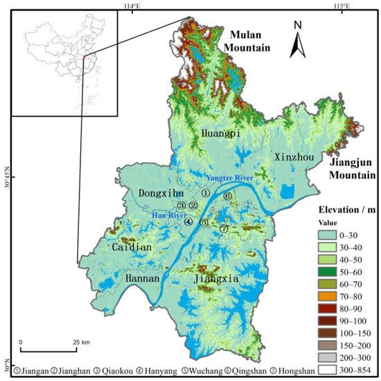
Figure 1.
Location of Wuhan city.
2.2. Data and Preprocessing
The data (Table 1) required for this study mainly include basic spatial data, remote sensing images, land use/cover, climate, population, GDP, and soil grid data from 2000 to 2020, as well as grid data for climate and socioeconomic forecasts under the SSP-RCP path of the CMIP6 model. In addition, there are socioeconomic statistical data from 2000 to 2020. Among them, the grid data come from relevant remote sensing image downloads or scientific data-sharing websites, and the socioeconomic statistical data come from statistical yearbooks over the years. Radiometric calibration and atmospheric correction were performed on remote sensing images using ENVI 5.3 software. The projections were unified and all vector and raster data were cropped to the same geographical range, with raster data uniformly set to a resolution of 30 m. Spatial correction was performed based on land use/cover data. The projection transformation, resampling, raster cropping, and other processing of vector and raster data were completed using ArcGIS 10.2 software. In addition, land use/cover data were categorized into six primary classes: cropland, forest, grassland, water bodies, impervious surfaces (construction land), and bare areas.

Table 1.
Overview of data sources and variables for land use and ecosystem quality assessment.
2.3. Methodology
2.3.1. Framework Overview
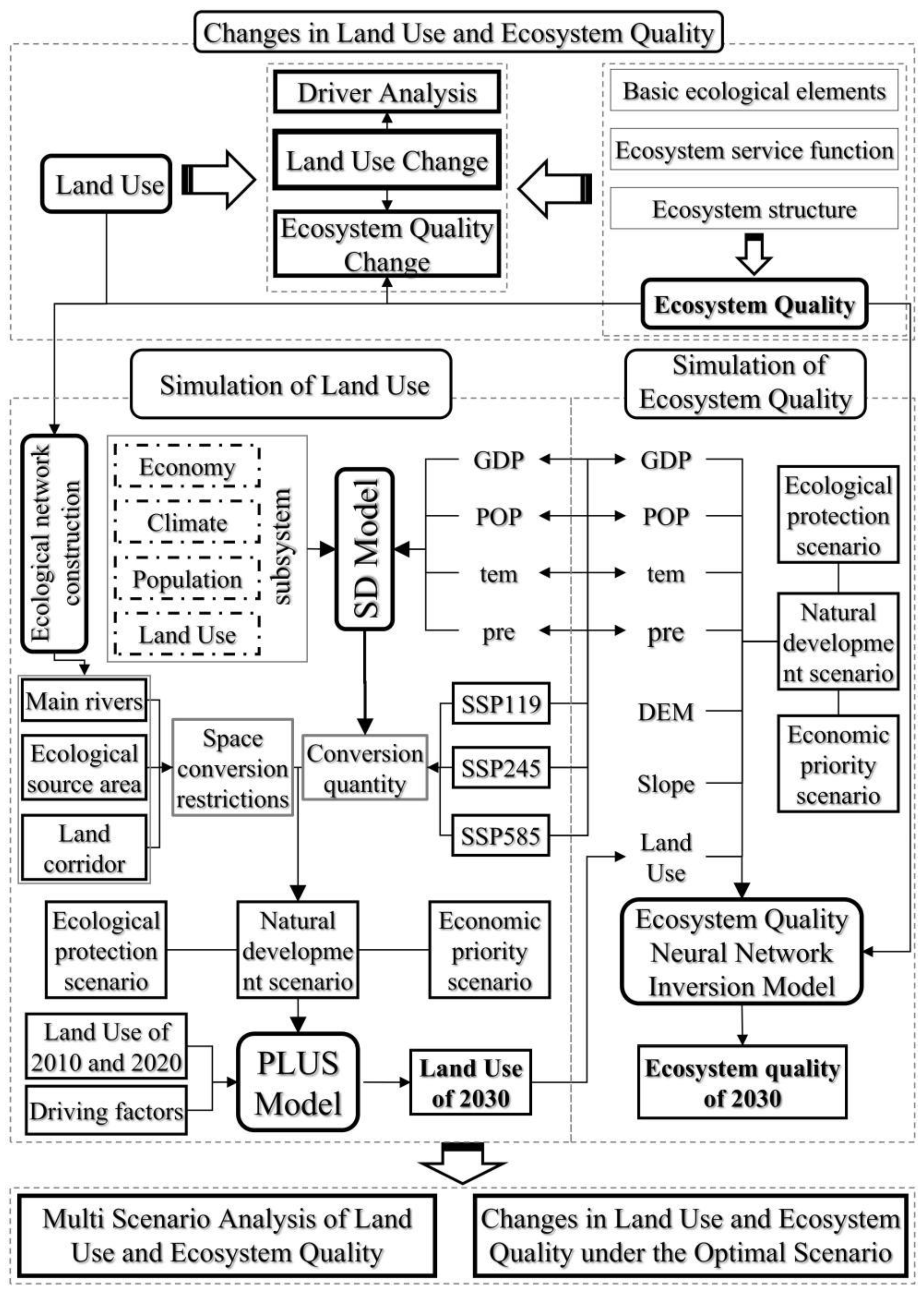
This study systematically examines land use changes and their driving factors from 2000 to 2020 while assessing ecosystem quality through three key dimensions: foundation, function, and structure. To project future ecological trends, three land use scenarios—ecological protection, natural development, and economic priority—were developed based on gross domestic product (GDP), population (POP), temperature (tem), and precipitation (pre) data from the SSP-RCP pathways of the CMIP6 model, alongside ecological network analysis. A system dynamics (SD) model, incorporating economic, population, climate, and land use subsystems, was constructed and integrated with the Patch-generating Land Use Simulation (PLUS) model to simulate multi-scenario land use changes in Wuhan for 2030. To evaluate ecosystem quality, a neural network-based inversion model was developed, using GDP, population, temperature, precipitation, elevation, slope, and land use/cover as independent variables. Under each scenario, ecosystem quality was predicted by inputting GDP, population, climate, and land use data while assuming elevation and slope remain constant. The final phase of the study involved a comprehensive multi-scenario analysis of land use and ecosystem quality, identifying the changes in land use and ecosystem quality from 2020 to 2030 and determining the optimal land use strategy. The overall methodological framework is illustrated in Figure 2.

Figure 2.
Integrated methodological framework for land use change analysis and ecosystem quality prediction.
2.3.2. Assessment of Ecosystem Quality
- (1)
- The “foundation-function-structure” framework for Ecosystem Quality Assessment
An ecosystem quality assessment system was constructed using the “foundation-function-structure” framework [29]. The foundation is indicated by a remote sensing ecological index that improves water area assessment [30], representing the state of ecological foundational elements such as vegetation, water, climate, and air quality. The function is represented by the comprehensive index of ecosystem service functions, which includes four types of service functions: Water Yield, Sediment Delivery Ratio, Carbon Storage, and Habitat Quality, calculated using InVEST 3.14.1. The structure is represented by the ecosystem organization force [31], which is composed of the Shannon’s Diversity Index, the area-weighted average patch fractal index, patch density, and the landscape contagion index, implemented using Fragstats V4.2.1. The calculation of indicator weights and objectives is completed based on ENVI 5.3 using the principal component analysis method, taking the first principal component (the eigenvalue contributions of PCA1 were all above 85%).
- (2)
- Grading system of Ecosystem Quality Change
The temporal dynamic monitoring of ecosystem quality is achieved by calculating the change in ecosystem quality (see Supplementary Figure S1) over a period of time, which characterizes ecosystem quality changes caused by land use changes [30,32]. The change in ecosystem quality is divided into seven levels: [−1~−0.5] for “Significantly worse”, (−0.5~−0.3] for “Obviously worse”, (−0.3~−0.1] for “Slightly worse”, (−0.1~0.1) for “No change”, [0.1~0.3) for “Slightly better”, [0.3~0.5) for “Obviously better”, and [0.5~1] for “Significantly better”.
2.3.3. Land Change Simulation Models
- (1)
- System Dynamics Model for land use quantity simulation
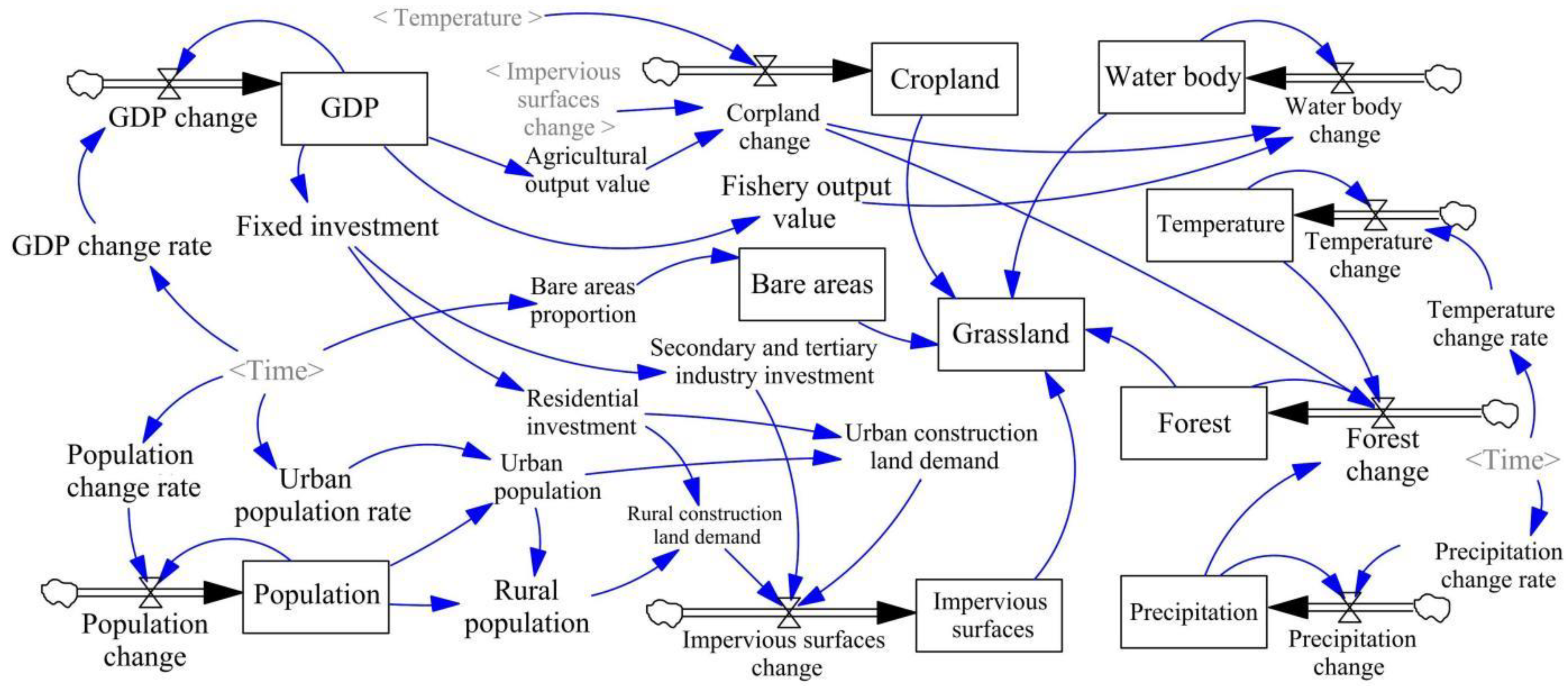
An SD model was constructed using Vensim PLE 7.3.5 for the simulation of land use quantity structure [14,29]. The spatial scope is Wuhan, the time period is from 2000 to 2030, and the simulation base year is 2000. Model validation is primarily based on historical data from the period 2000–2020. The time unit for model operation is one year. The SD model encompasses land, population, economic, and climate subsystems. The economic subsystem is represented by gross domestic product (GDP), the population subsystem is represented by the population count, and the climate subsystem is represented by temperature and precipitation. The land subsystem includes six categories: cropland, forest, grassland, water bodies, impervious surfaces, and bare areas. The constructed SD model (Figure 3) involves 33 variables, with the causal relationships between variables quantitatively expressed through mathematical equations. The rates of change for population, GDP, temperature, and precipitation are calculated based on historical data, while future data are treated as multi-scenario parameters [29].
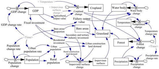
Figure 3.
Conceptual framework of the system dynamics model for land use quantity evolution and its interactions with socioeconomic and climate factors.
The simulation accuracy is specifically tested through the deviation area between the simulated and observed values of land use quantity structure. In the years 2000, 2005, 2010, 2015, and 2020, the total deviation areas were 0.00, 91.12, 114.16, 138.91, and 23.92 square kilometers, respectively, with overall deviation ratios of 0.00%, 1.06%, 1.33%, 1.62%, and 0.28%. The total deviation area and the overall deviation ratio are relatively small, indicating that the constructed SD model is sufficiently accurate and can effectively simulate and predict the quantity structure of land use.
- (2)
- Designation of multiple scenarios based on SSP-RCP pathways
Using the population, GDP, temperature, and precipitation data [25,26,27,28] under the SSP119, SSP245, and SSP585 scenarios [29] of the CMIP6 model’s SSP-RCP pathways, the annual average rates of change for population, GDP, temperature, and precipitation from 2020 to 2030 were calculated. These rates serve as parameters (Table 2) for the SD model under the three scenarios to simulate and predict the land use quantity structure (Table 3) for the year 2030 under different scenarios.
Table 2.
Projected annual change rates of key socioeconomic and climate variables under different land use scenarios (2020–2030) (%).
Table 3.
Projected land quantities under different scenarios in Wuhan for 2030 (km2).
Based on the constructed ecological network [29] (ecological source areas, strategic nodes, and corridors) (see Supplementary Figure S2), the land use conversion spatial baseline range was differentially set according to the ecological importance (Table 4). Combined with the SSP119, SSP245, and SSP585 scenarios, three scenarios were formed from two aspects: land use quantity structure and spatial simulation baseline restrictions—ecological protection, natural development, and economic priority.
Table 4.
Comparative designation of multi-scenario land use simulation: ecological protection, natural development, and economic priority.
- (3)
- Land change allocation based on the Patch-generating Land Use Simulation Model
Referring to the relevant studies [15,29], based on land use data from 2010 and 2020, the Patch-generating Land Use Simulation (PLUS) model was constructed. The LEAS module calculates the contribution of driving factors and analyzes land expansion strategies to obtain the development probability for each type of land use. Based on the land use development probability and the target year’s land use quantity structure, the CARS module simulates the spatial layout of land use. The land use simulation results for 2020 are compared with the actual land use data. The overall land use layout (see Supplementary Figure S3) is essentially the same, with a Kappa coefficient of 0.81 and a FoM coefficient of 0.18. The constructed PLUS model has a high degree of accuracy and can be used for the multi-scenario simulation of land use changes for the year 2030.
2.3.4. Ecosystem Quality Prediction Under Different Scenarios Using Neural Network Model
Taking ecosystem quality as the dependent variable and land use structure ecological index (LUSEI) [29], ecosystem organization force (EO), elevation (DEM), slope (Slope), precipitation (pre), temperature (tmp), population (POP), and GDP as independent variables, sample point data collection for Wuhan was conducted using a 1000 × 1000 m grid. A total of 42,870 sample point data were collected for the years 2000, 2005, 2010, 2015, and 2020. Randomly, 50% of the samples were selected as the training set (Training), 25% as the validation set (Validation), and 25% as the testing set (Testing). The number of hidden layer neurons was set to the default value of 10, and the network training function was trainlm [29]. Using the neural network fitting toolbox in MATLAB 2020a, an ecosystem quality neural network inversion model was constructed (Table 5).
Table 5.
Performance evaluation of the ecosystem quality neural network inversion model and mapping accuracy across different time periods.
Based on the trained ecosystem quality neural network inversion model and the independent variable raster datasets for the years 2000, 2005, 2010, 2015, and 2020, MATLAB 2020a programming was used to implement the reading and calculation of independent variable raster data, and to invert and map the ecosystem quality for the years 2000, 2005, 2010, 2015, and 2020. The actual ecosystem quality assessment maps and the inversion mapping results for the years 2000, 2005, 2010, 2015, and 2020 were subjected to correlation analysis between two raster layers involving all pixels (30 × 30 m, 4452 × 5152). The correlation coefficient R for each year was close to 0.9 (Table 5), which also matches the model accuracy.
Furthermore, all independent variables of the ecosystem quality neural network inversion model can be obtained under the ecological protection, natural development, and economic priority scenarios. Among them, LUSEI and EO are calculated from land use simulation data, while tmp, pre, POP, and GDP are derived from the SSP119, SSP245, and SSP585 scenarios. DEM and Slope are considered constant. Therefore, it is possible to achieve a multi-scenario simulation of ecosystem quality for Wuhan in 2030.
3. Results and Analysis
3.1. Changes in Land and Ecosystem Quality from 2000 to 2020
3.1.1. Land Change from 2000 to 2020 in the Study Area
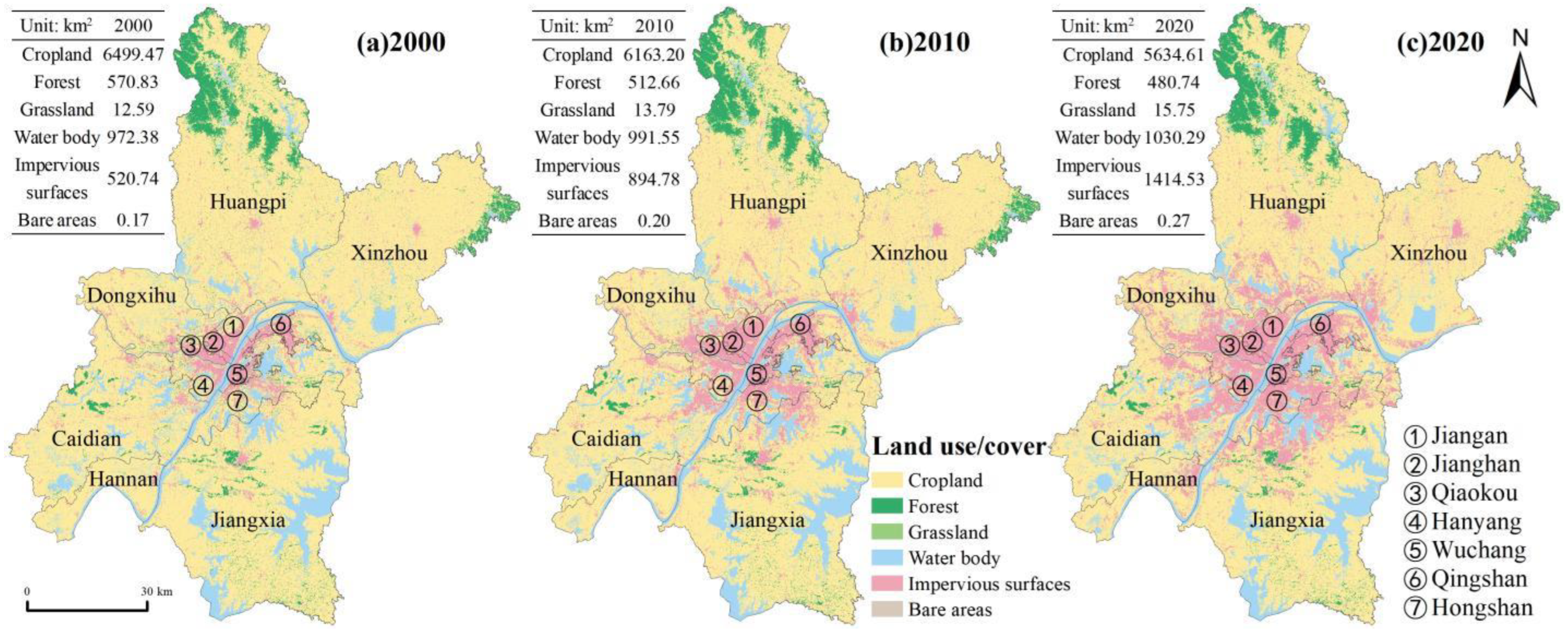
From 2000 to 2020, land use changes were primarily characterized by the decrease in cropland and the increase in impervious surfaces. Cropland decreased from 6499.47 km2 to 5634.61 km2, while impervious surfaces increased from 520.74 km2 to 1414.53 km2. Additionally, there was a slight increase in water body area (from 972.38 km2 to 1030.29 km2) and a decrease in forest (from 570.83 km2 to 480.74 km2). Grassland and bare areas had minimal proportions and changes. Spatially (Figure 4), land use changes were mainly concentrated on the periphery of the central urban area, primarily due to urban expansion leading to the reduction in cropland.
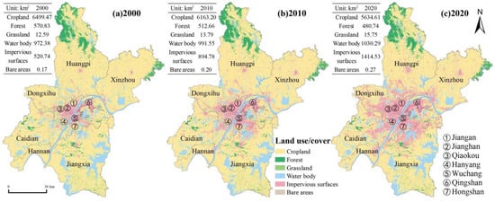
Figure 4.
Spatial distribution and temporal changes in land use patterns (2000–2020).
From the land use transfer matrix (Table 6), the types with a transfer area exceeding 10 km2 include “Cropland-Forest (C-F)”, “Cropland-Water body (C-W)”, “Cropland-Impervious surfaces (C-I)”, “Forest-Cropland (F-C)”, “Forest-Impervious surfaces (F-I)”, and “Water body-Cropland (W-C)”. Among these, “C-I” is the most significant transfer type, with its transfer area from 2010 to 2020 increasing by nearly half compared to 2000 to 2010. Additionally, there were small-scale area transfers for “Cropland-Grassland (C-G)”, “Forest-Water body (F-W)”, “Water body-Forest (W-F)”, and “Water body-Impervious surfaces (W-I)”, where the transfer area for “W-I” exceeded 5 km2 and that for “F-W” exceeded 2 km2. The rest had areas close to or less than 1 km2. The reduction in cropland mainly involves urban expansion and reforestation or returning farmland to lakes. The decrease in forest land mainly involves the reclamation of arable land and urban expansion. The reduction in water body area is mainly due to land reclamation around lakes. Among them, the rate of reduction in forest and water body areas from 2000 to 2010 was significantly higher than that from 2010 to 2020.
Table 6.
Land Use Transfer Matrix for 2000–2010–2020.
3.1.2. Drivers of Land Changes in the Study Area
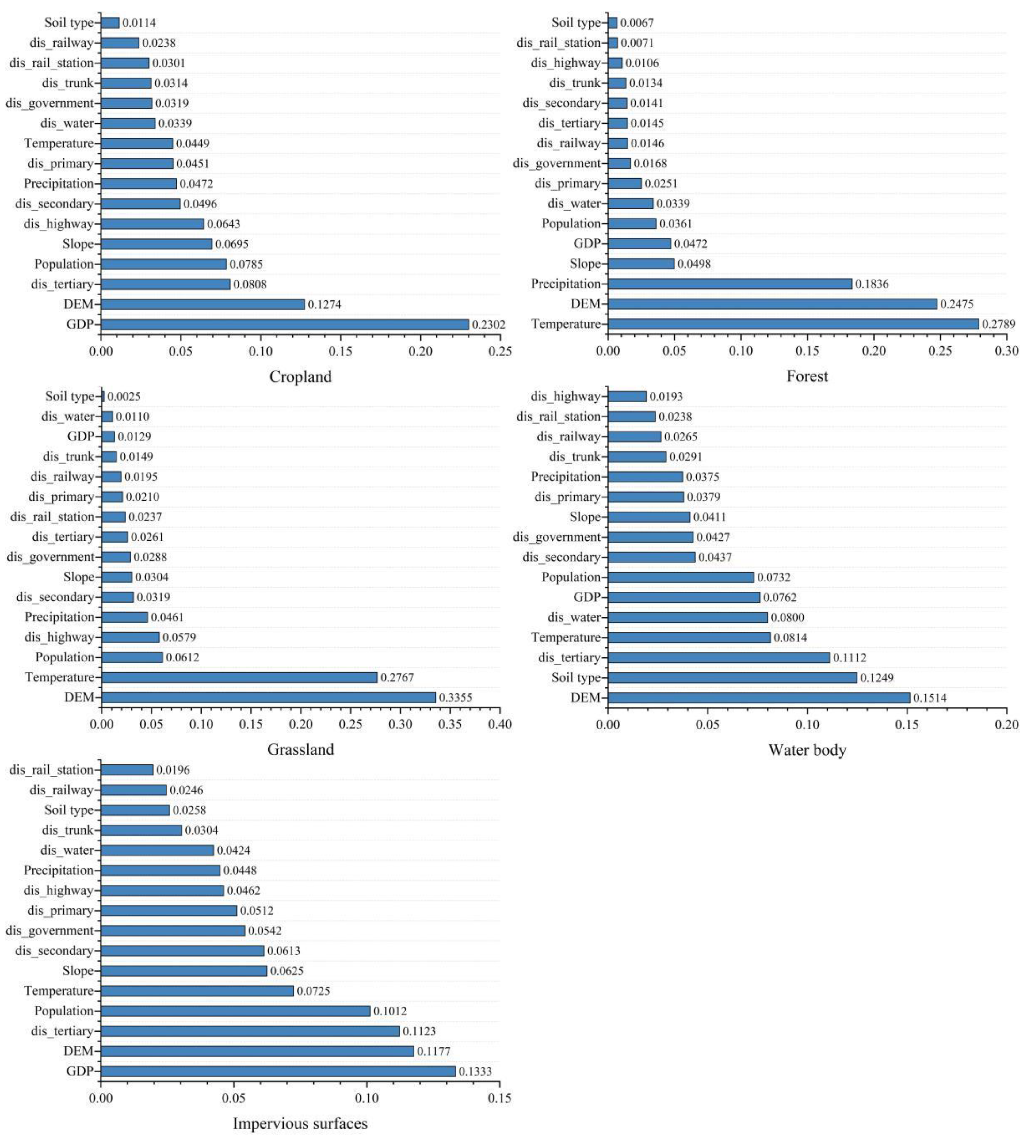
Analyzing the contributions of different driving factors for various types of land use through the LEAS module of the PLUS model (Figure 5), the changes in impervious surfaces are mainly influenced by GDP, elevation, distance to tertiary roads, and population. Economic development increases impervious surfaces demand, while terrain restricts its direction and extent. The layout of impervious surfaces is closely related to the distribution of the transportation network, with tertiary roads being the main force in the expansion of the road network. The changes in cropland are mainly affected by GDP and elevation. Economic development can lead to the conversion of cropland to impervious surfaces, while also increasing investment for the reclamation and supplementation of cropland. Elevation is the most direct limiting factor for the reclamation of cropland. The changes in forest are mainly influenced by temperature, elevation, and precipitation. The growth and distribution of vegetation are significantly affected by temperature, precipitation, and elevation. The changes in grassland are also mainly influenced by elevation and temperature. However, due to the small area and fragmented patches of grassland, the demand for artificial irrigation is higher, and thus the dependence on precipitation is relatively lower. The changes in water body areas are mainly influenced by elevation, soil type, and distance to tertiary roads. Terrain and the distribution of the tertiary road network to some extent restrict the expansion of water body areas, and there is a certain pattern between soil type and the spatial distribution of water body areas. (Bare areas have an area of less than 1 km2 and are not analyzed).

Figure 5.
Relative contributions of key driving factors to different land use changes in Wuhan (2000–2020). (“dis” is an abbreviation of “distance”; “primary/secondary/tertiary” represents three levels of roads).
3.1.3. Ecosystem Quality Change from 2000 to 2020 in the Land Change Area
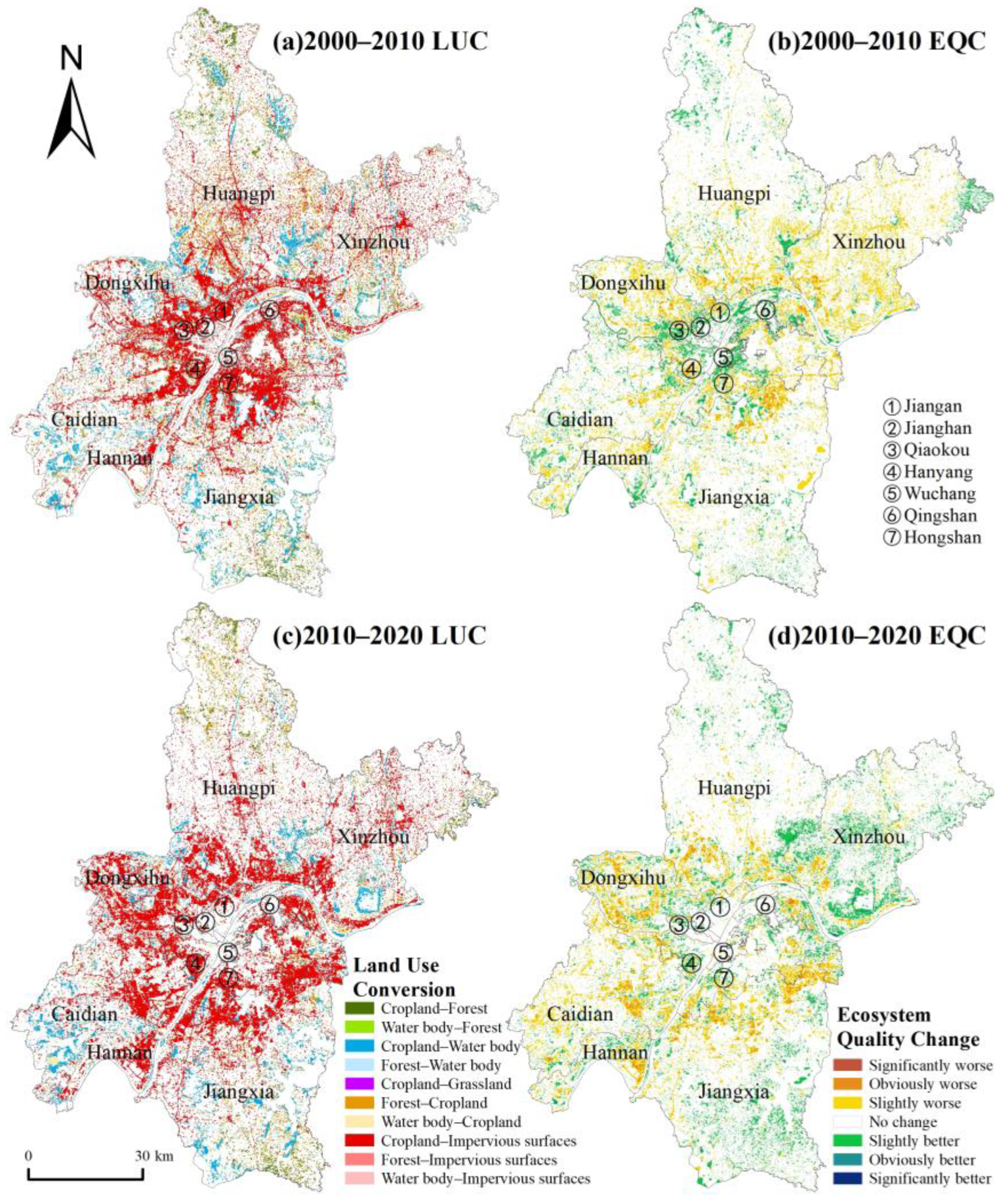
From 2000 to 2010 to 2020, land use conversion types with an area greater than 1 km2 include “C-F”, “C-W”, “C-I”, “F-C”, “F-I”, “W-C”, “C-G”, “F-W”, “W-F”, and “W-I” (Table 6 and Figure 6a,c). Among them, “C-I” has the largest area and the widest distribution, mainly located in the peripheral areas of towns and in the interlaced zones of construction and agricultural land; “C-W” also has a relatively large area, concentrated around lake waters, and is the result of converting cropland back to lakes. The areas of “F-C” and “W-C” are also relatively large, but their distribution is more scattered, often involving small-scale, fragmented patches of forest or water areas being reclaimed as cropland. A certain area of “C-F” is scattered in the northern Mulan Mountain and eastern Jiangjun Mountain areas; other conversion types have relatively smaller areas and are not significantly distributed in space. Combining the changes in ecosystem quality from 2000 to 2010 and to 2020 (Figure 6b,d), the areas of land use conversion are also the main areas where ecosystem quality changes. The outer side of the peripheral areas of the central urban area is the main area where ecosystem quality decreases, while the inner side shows a trend of improving ecosystem quality. This is mainly due to the conversion of land use types causing changes in spatial structural stability, with the outer side decreasing and the inner side increasing.
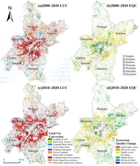
Figure 6.
Spatial distribution of land use conversion and ecosystem quality change from 2000 to 2020.
Specific analysis of the changes in ecosystem quality within the scope of various types of land use conversion (Table 7) shows that the area of “C-I” is the largest, and the change in ecosystem quality within its range is also the greatest; the area of “Slightly worse” reaches 49–55% of the transformed area, and the area of “Obviously worse” reaches 15–21%. From 2000 to 2010, over 64% of the area within “C-I” experienced a decline in ecosystem quality; from 2010 to 2020, over 76% of the area within “C-I” experienced a decline in ecosystem quality. In the smaller areas of “F-I” and “W-I”, “Slightly worse” and “Obviously worse” are also the main manifestations, overall showing a result of deteriorating ecosystem quality. Moreover, in the areas of “C-F” and “C-W”, “No change”, “Slightly better”, and “Obviously better” are predominant, overall showing an improvement in ecosystem quality. In contrast, “F-C” and “W-C” areas are mainly characterized by “No change”, “Slightly worse”, and “Obviously worse”, overall indicating a decline in ecosystem quality.
Table 7.
Ecological impact of land use conversion types from 2000 to 2020: changes in ecosystem quality across different land conversions.
3.2. Simulation of Land Use and Ecosystem Quality Under Different Scenarios
3.2.1. Land Use and Ecosystem Quality Simulation
- (1)
- Land Use Simulation
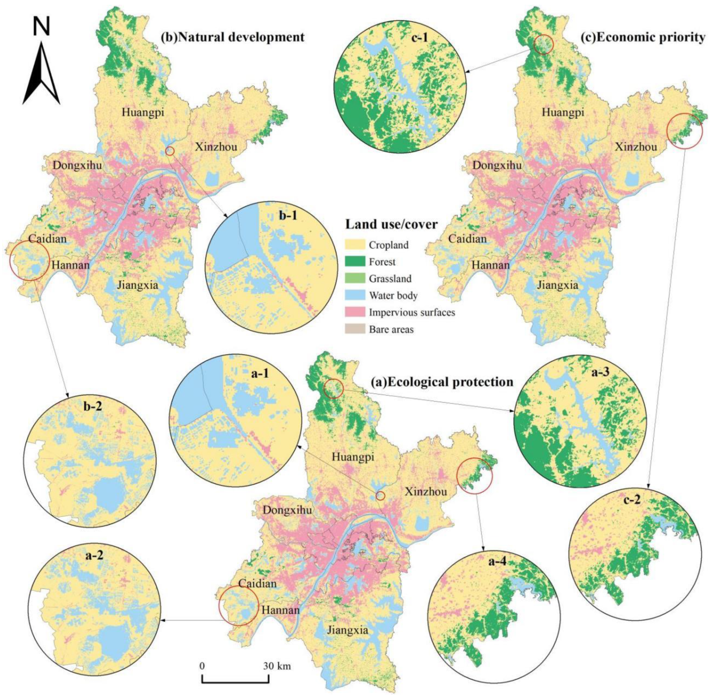
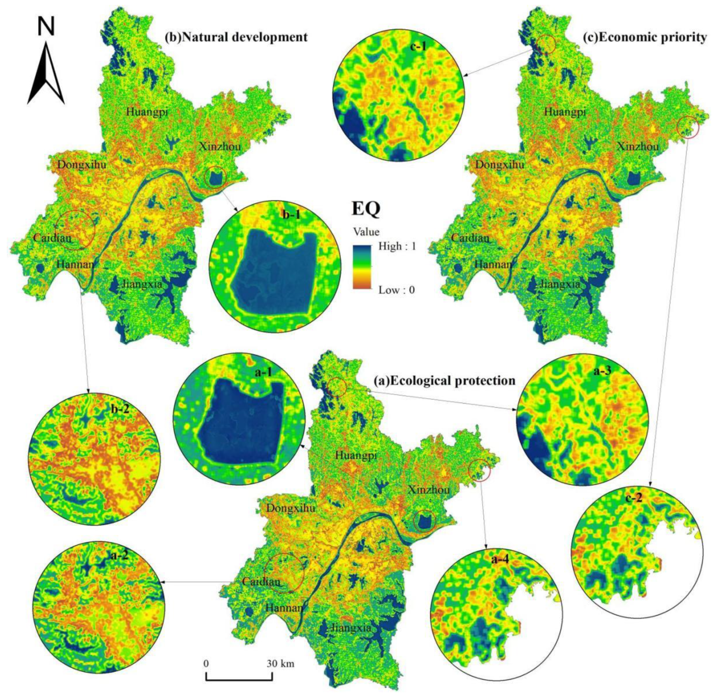
From the perspective of spatial structure characteristics (Figure 7), the simulated land use results for Wuhan in 2030 under the scenarios of ecological protection, natural development, and economic priority have a basically consistent overall layout. However, there are obvious differences in the detailed spatial distribution features of land categories. Among them, the impervious surfaces and cropland under the three scenarios mainly show differences in patch edge ranges due to different areas, while the distribution layout and patch detail features are essentially consistent. In terms of ecological land use, the areas of forest and water bodies under different scenarios are relatively similar, but there are significant differences in patch detail features. Compared to the ecological protection scenario, the ecological land use, especially water body patches, in the natural development scenario is more severely eroded by surrounding land types, mainly cropland, leading to a reduction in the range of water bodies and other ecological land use patches and more fragmented edges. This is particularly evident in Wu Lake (Figure 7(a-1,b-1)) and the southwestern region with dense lakes and marshes (Figure 7(a-2,b-2)). Overall, the overall land use layout under the three scenarios is essentially consistent, with minimal differences in patch detail features for impervious surfaces and cropland. However, the water body and forest patches under the ecological protection scenario are more intact, avoiding the fragmentation of patches and the proliferation of small patches; that is, the spatial structure of ecological land use under the ecological protection scenario is superior to that of the other two scenarios.
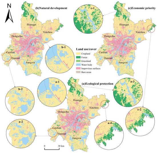
Figure 7.
Spatial distribution of land use under multi-scenario simulations for Wuhan in 2030. (a-1–a-4, b-1–b-2, and c-1–c-2 show the detailed features of local areas).
From the land use conversion situation (Table 8), under the economic priority scenario, the transfer of cropland, forest, and water body areas to impervious surfaces is predominant, with “C-I” accounting for the vast majority. The conversion between cropland and water body areas is secondary, with “C-W” accounting for the vast majority. Under the natural development and ecological protection scenarios, the situation of impervious surfaces transfer and the conversion between cropland and water body areas is similar. In addition, there is a small amount of cropland and grassland being converted to forest, as well as a small amount of forest being converted to cropland and water body areas. Comparing between different scenarios, the transfer to impervious surfaces is the highest under the economic priority scenario, followed by the ecological protection scenario, and the least under the natural development scenario. The comparison of “C-W” and “W-C” is also similar. In addition, compared to the economic priority scenario, the land use conversion types under the natural development and ecological protection scenarios are richer, with increased conversions between cropland, forest, and grassland. The area of “C-F” is higher under the ecological protection scenario than under the natural development scenario, while the areas of “F-C”, “F-W”, and “Grassland-Forest (G-F)” are essentially consistent.
Table 8.
Land use conversion across different scenarios from 2020 to 2030 (for land use changes ≥ 1 km2).
- (2)
- Ecosystem Quality predictions
As can be seen from Figure 8, the overall spatial pattern of ecosystem quality under the three scenarios of ecological protection, natural development, and economic priority is essentially consistent and corresponds with the spatial distribution of land use. Furthermore, the ecosystem quality under the ecological protection scenario is higher, and its spatial structure details are superior to the other two scenarios. In particular, the ecosystem quality at the urban periphery (Figure 8(a-2,b-2)) is significantly higher under the ecological protection scenario than under the natural development scenario. The ecosystem quality of lake waters (Figure 8(a-1,b-1)) is slightly higher under the ecological protection scenario than under the natural development scenario. The fragmentation of ecological land patches leads to lower ecosystem quality in some areas under the economic priority scenario compared to the ecological protection scenario (Figure 8(a-3,a-4,c-1,c-2)). In addition, the average ecosystem quality under the ecological protection, natural development, and economic priority scenarios is 0.52, 0.50, and 0.50, respectively. Therefore, the ecosystem quality in 2030 under the ecological protection scenario is the highest overall and has the best spatial distribution structure characteristics, which can serve as a reference for the expected changes in ecosystem quality.

Figure 8.
Predicted ecosystem quality under multi-scenario simulations for Wuhan in 2030. (a-1–a-4, b-1–b-2, and c-1–c-2 show the detailed features of local areas).
3.2.2. Changes in Land Use and Ecosystem Quality Under Optimal Scenario
As known from Section 3.2.1, the simulation results of land use and ecosystem quality under the ecological protection scenario are the best. Therefore, this section predicts and analyzes the possible ecosystem quality changes in the optimal land use conversion from 2020 to 2030 by comparing the land use conversion (types with area ≥ 1 km2) and the degree of ecosystem quality change under the ecological protection scenario.
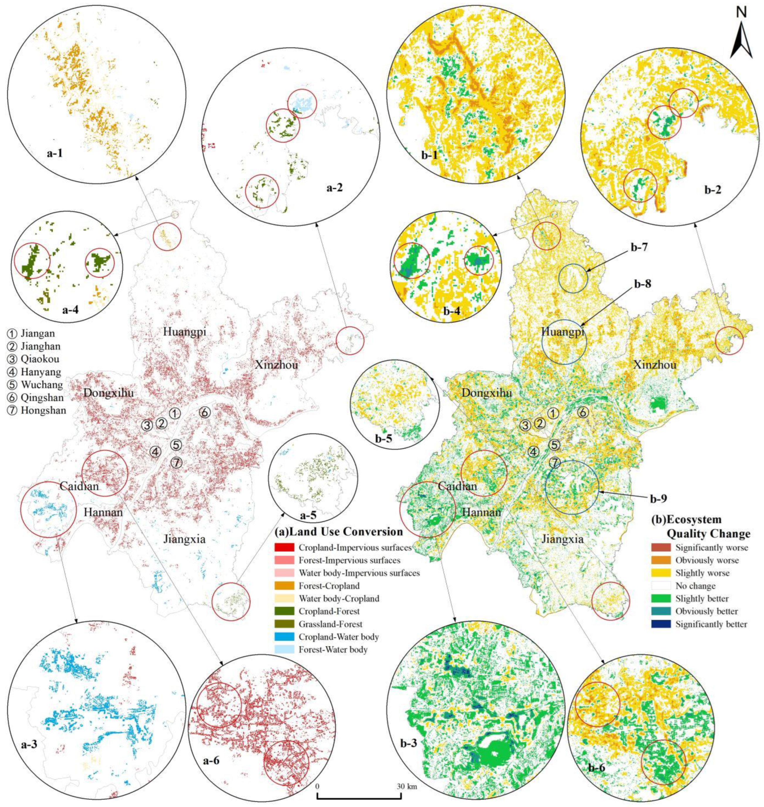
From the spatial distribution (Figure 9), “C-I” is mainly distributed around the central urban area and the periphery of major towns, with some “C-W” in the southwestern part of Caidian. Other conversion types, due to their small area and scattered distribution, do not have obvious clustered areas. The decline in ecosystem quality is mainly caused by urban expansion and the encroachment of forest and grassland areas, with the decline occurring primarily at the edges of towns and ecological land use areas. The improvement in ecosystem quality is mainly due to two reasons: one is the conversion of the early urban edge land space conflict areas into stable areas inside the urban edge, and the other is the integration and expansion of fragmented ecological land patches such as water bodies and wetlands. Therefore, ecosystem quality can effectively be enhanced by, on one hand, improving the utilization rate of urban edge land conflict areas and controlling their scope, and on the other hand, integrating fragmented ecological land patches and perfecting their landscape spatial structure.
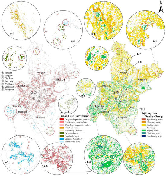
Figure 9.
Land use conversion and ecosystem quality change under the ecological protection scenario from 2020 to 2030. (a-1–a-6, and b-1–b-6 show the detailed features of local areas).
Specifically comparing local features (Figure 9), it is found that the conversion of fragmented forest in the gaps of cropland patches to cropland, reducing the small patches of fragmented forest (Figure 9(a-1,b-1)), can optimize the landscape spatial structure of cropland and enhance ecosystem quality. Implementing the conversion of cropland to forest, transforming cropland in the gaps of forest patches into forest (Figure 9(a-2,a-4,b-2,b-4)), can optimize the landscape spatial structure of forest, improve vegetation quality, and effectively enhance ecosystem quality. Carrying out the conversion of cropland to lakes, transforming cropland around water body areas into water bodies (Figure 9(a-3,b-3)), increases area and improves the landscape spatial structure of water body areas, which can effectively enhance ecosystem quality. Furthermore, in situations where there are a large number of fragmented forest patches distributed within cropland, converting some cropland adjacent to forest into forest (Figure 9(a-5,b-5)) will further reduce the connectivity of the landscape spatial structure, increase heterogeneity, and thereby decrease local ecosystem quality. “F-W” to some extent will lead to a decrease in ecosystem quality (Figure 9(a-2,b-2)). “C-I” has two impacts on ecosystem quality (Figure 9(a-6,b-6)). One is in the expansion areas at the urban periphery, where “C-I” intensifies land use conflicts, complicates the landscape spatial structure, and reduces the natural foundation quality, thereby significantly decreasing ecosystem quality. The other is within the urban area, especially on the inner side of the urban periphery, where “C-I” improves the landscape spatial structure of land use, alleviates or even eliminates the fragmentation of land patches, and reduces land use conflicts, effectively enhancing ecosystem quality.
Statistical analysis of the changes in ecosystem quality due to land use conversion types (Table 9) reveals that “C-I” has the largest area and also the greatest change in ecosystem quality; the area of “Slightly worse” is 49.96%, and the area of “Obviously worse” is 6.58%. Over 55% of the area within “C-I” experiences a decline in ecosystem quality. For the smaller areas of “F-I” and “W-I”, the changes in ecosystem quality are also mainly characterized by “Slightly worse” and “Obviously worse”, overall showing a deteriorating result. The area of “C-W” is second only to “C-I”, with “Slightly better” accounting for 27.44% of the area, “Obviously better” for 15.58%, and “Significantly better” for 3.16%. Over 45% of the area within “C-W” shows an improvement in ecosystem quality. In addition, the changes in ecosystem quality for “F-C” and “W-C” are mainly characterized by “No change”, “Slightly worse”, and “Obviously worse”, overall showing a deteriorating result. “C-F”, “G-F”, and “F-W” also overall show a deteriorating result in ecosystem quality.
Table 9.
Land use conversion and ecosystem quality change under the ecological protection scenario from 2020 to 2030.
4. Discussion
This paper constructs an ecosystem quality assessment system based on the “foundation-function-structure” framework, integrating the remote sensing ecological index that improves water area assessment (WIRSEI), the comprehensive index of ecosystem service functions (ESFs), and ecosystem organization (EO) force. Compared with remote sensing ecological indices [3], landscape ecological quality [4], ecological risk [5], ecological security [6], ecosystem services [7,8] and ecosystem health [9], etc., the indicators of the assessment system are more comprehensive and can effectively characterize ecosystem quality. The assessment indicators can achieve high-precision raster expression, and the indicator data can meet the requirements for regular updates. Furthermore, through the SD-PLUS land use simulation model, the ecosystem quality neural network inversion model, and the multi-scenario parameters of the CMIP6 model’s SSP-RCP pathways, the paper achieves simulation and prediction from land use to ecosystem quality. The research approach utilizes the inversion model to combine ecosystem quality with influencing factors that can be subjected to multi-scenario simulation (such as land use, temperature, precipitation, GDP, and population), achieving a research framework design from multi-scenario parameters of influencing factors to multi-scenario inversion of ecosystem quality. It also effectively integrates the land use simulation results with climate, economic, and population elements under corresponding scenarios. This shifts from using land use simulation results alone to predict ecological conditions in a single dimension, such as habitat quality [10], remote sensing ecological index [11], and ecological risk [12,13], to using multiple simulated elements to predict a more comprehensive ecosystem quality. This is an innovative application approach in the inversion of ecosystem quality and land use simulation methods, providing new references for related studies.
In the economic priority scenario, the demand for impervious surfaces is the highest, leading to a large amount of cropland and some ecological land being transferred in, while in the ecological protection scenario, the demand for impervious surfaces is lower than in the economic priority scenario but higher than in the natural development scenario. This indicates that the degree of urban construction in the ecological protection scenario, although not as high as in the economic priority scenario, is higher than in the natural development scenario, and this is also the case with the level of economic development. Under the new era of ecological civilization, in addition to the level of economic development, there is a greater pursuit of ecological standards. This is not only about increasing the volume of development, but also about enhancing the quality of development. Compared to the natural development and economic priority scenarios, the fact that more forest land, grassland, and water areas are transferred in under the ecological protection scenario indicates better ecological quality. The ecological protection scenario balances economic development and ecological quality, and is superior to the other two scenarios in terms of land use conversion. It aligns with the development direction under the current policy context and meets the requirements of ecological civilization construction and sustainable development.
In the optimal (ecological protection) scenario of land use simulation, there are two reasons why land use conversion affects ecosystem quality. One is by changing the natural foundation through land type conversion, and the other is by altering the landscape structure through land type conversion. Among them, there are four types of land use conversions that lead to an increase in ecosystem quality: first, the conversion of cropland in the gaps of forest to forest (afforestation); second, the conversion of cropland at the edges of water body areas that have been eroded to water bodies (lake restoration); third, the reclamation of fragmented forest and grassland within the range of cropland to cropland; and fourth, the conversion of fragmented cropland within urban areas to impervious surfaces. There are three types of land use conversions that lead to a decrease in ecosystem quality: first, the expansion of urban areas and the conversion of cropland to impervious surfaces; second, the conversion of forest at the edges of water bodies within forest to water body areas; and third, the increase or expansion of fragmented patches of other land types within the range of cropland. Therefore, in the process of future land use conversion in Wuhan, it is necessary to strengthen the guidance and control of land use conversion in these areas, and try to promote the four types of ecosystem quality increases and avoid the three types of ecosystem quality decreases. In addition, these main land type conversion areas that affect changes in ecosystem quality can serve as one of the effective references for whether ecological restoration is needed.
In this study, the weights and calculation methods of the assessment system indicators are based on principal component analysis. In future research, other methods can be attempted, and the impact of different methods on the assessment results can be analyzed. The assessment system still needs to be further improved and optimized. Due to insufficient understanding of the development patterns of the population, economy, land, and climate subsystems involved in land use conversion, as well as their mutual coupling and feedback mechanisms, the constructed system dynamics model of land use quantity structure evolution still needs to be further improved. In the next step, it is possible to consider incorporating management and policy-related factors into the SD model, and to take into account the differences in the evolution of land use quantity structure between different administrative levels and at the same level. In addition, affected by the uncertainty of future climate and socioeconomic predictions, there is potential deviation in the land use simulation results. That is, the land use, climate, economic, and population data under future scenarios all have certain deviations. The deviation in the accuracy of the ecosystem quality inversion model can be calculated, while the deviation in the multi-scenario assessment and prediction of ecosystem quality caused by the deviation of future scenario data is difficult to calculate. In the next step, it is considered to analyze the differences between multi-scenario data and measured data of historical years as a reference before multi-scenario assessment and prediction of ecosystem quality, in the hope of improving the impact of uncertainty in multi-scenario future data on the assessment and prediction of ecosystem quality. Finally, the ecosystem quality inversion model assumes that the altitude and slope remain unchanged. This has little impact on small and medium-scale areas with small topographical differences and changes, but has a greater impact on large-scale areas with large topographical differences or changes.
5. Conclusions
This study comprehensively analyzed and assessed the land use changes in Wuhan from 2000 to 2020 and the resulting changes in ecosystem quality, and projected future ecosystem quality under different land use scenarios for 2030. By employing a “foundation-function-structure” framework, system dynamics (SD), the Patch-generating Land Use Simulation (PLUS) model, and an ecosystem quality neural network inversion model, this research provided a robust methodological approach for evaluating and predicting land use-driven ecological changes.
The results indicate that rapid urban expansion has significantly influenced land use transitions, particularly the conversion of cropland to impervious surfaces, leading to declines in ecosystem quality. Over the past two decades, Wuhan has experienced a marked decrease in cropland and forest areas, while water bodies have slightly expanded. These changes have resulted in both positive and negative ecological effects, depending on the specific land use conversions. The simulation results for 2030 suggest that under the ecological protection scenario, ecosystem quality would be optimized, with more stable landscape structures and reduced fragmentation of ecological land patches. In contrast, the economic priority scenario would lead to further urban expansion, increasing ecological stress and reducing ecosystem quality in several key areas. The comparative analysis of multiple scenarios highlights the importance of balancing economic development with ecological sustainability. The ecological protection scenario emerges as the most favorable option, aligning with the principles of sustainable development and ecological civilization. Under the ecological protection scenario from 2020 to 2023, the expansion of the central urban area and the edges of major towns, as well as the erosion of some forest and grassland areas, led to a decrease in ecosystem quality. In contrast, the integration and expansion of fragmented ecological patches such as water bodies and wetlands in the southwest of Caidian, and the transformation of early urban edge conflict zones into stable interior areas of the urban edge, resulted in an increase in ecosystem quality. This scenario demonstrates that strategic land use planning, and integrating conservation policies with controlled urban expansion, can significantly mitigate ecological degradation while ensuring economic growth.
Despite this study’s contributions, challenges remain in refining predictive models and incorporating more dynamic socioeconomic and policy factors. Future research should focus on enhancing the integration of high-resolution geospatial data, refining ecosystem quality assessment indicators, and incorporating real-time environmental monitoring. Additionally, improved policy-oriented simulations could offer more actionable insights for urban planners and policymakers.
Supplementary Materials
The following supporting information can be downloaded at: https://www.mdpi.com/article/10.3390/land14030515/s1, Figure S1. Spatial Distribution and Temporal Changes in Ecosystem Quality (2000–2020); Figure S2. Ecological network pattern; Figure S3. Land use layout of 2020 (a. Actual; b. Simulated).
Author Contributions
Conceptualization, Y.P.; Data curation, J.G.; Methodology, Y.P.; Software, Y.P.; Visualization, Y.P.; Writing–original draft, Y.P.; Writing–review and editing, J.Y. All authors have read and agreed to the published version of the manuscript.
Funding
This work was supported by the National Natural Science Foundation of China (42101275).
Data Availability Statement
The original contributions presented in the study are included in the article, further inquiries can be directed to the corresponding author.
Conflicts of Interest
The authors declare no conflicts of interest.
References
- Kong, X.; Fu, M.; Zhao, X.; Wang, J.; Jiang, P. Ecological effects of land-use change on two sides of the Hu Huanyong Line in China. Land Use Policy 2022, 113, 105895. [Google Scholar] [CrossRef]
- Song, X.-P.; Hansen, M.C.; Stehman, S.V.; Potapov, P.V.; Tyukavina, A.; Vermote, E.F.; Townshend, J.R. Global land change from 1982 to 2016. Nature 2018, 560, 639–643. [Google Scholar] [CrossRef] [PubMed]
- Firozjaei, M.K.; Fathololoumi, S.; Weng, Q.; Kiavarz, M.; Alavipanah, S.K. Remotely Sensed Urban Surface Ecological Index (RSUSEI): An Analytical Framework for Assessing the Surface Ecological Status in Urban Environments. Remote Sens. 2020, 12, 2029. [Google Scholar] [CrossRef]
- Wu, Z.; Zhu, D.; Xiong, K.; Wang, X. Dynamics of landscape ecological quality based on benefit evaluation coupled with the rocky desertification control in South China Karst. Ecol. Indic. 2022, 138, 108870. [Google Scholar] [CrossRef]
- Hasan, M.; al Ahmed, A.; Islam, A.; Rahman, M. Heavy metal pollution and ecological risk assessment in the surface water from a marine protected area, Swatch of No Ground, north-western part of the Bay of Bengal. Reg. Stud. Mar. Sci. 2022, 52, 102278. [Google Scholar] [CrossRef]
- Nan, B.; Zhai, Y.; Wang, M.; Wang, H.; Cui, B. Ecological Security Assessment, Prediction, and Zoning Management: An Integrated Analytical Framework. Engineering 2024, in press. [CrossRef]
- Kwak, Y.; Chen, S. Integrating seasonal climate variability and spatial accessibility in ecosystem service value assessment for optimized NbS allocation. Urban Clim. 2025, 59, 102314. [Google Scholar] [CrossRef]
- Wang, Q.; Bai, X. Spatiotemporal characteristics of human activity and land use on ecosystem service functions in mountainous areas of Northeast Guizhou, Southwest China. Ecol. Eng. 2025, 212, 107473. [Google Scholar] [CrossRef]
- Bi, X.; Fu, Y.; Wang, P.; Zhang, Y.; Yang, Z.; Hou, F.; Li, B. Ecosystem health assessment based on deep learning in a mountain-basin system in Central Asia’s arid regions, China. Ecol. Indic. 2024, 165, 112148. [Google Scholar] [CrossRef]
- Wang, B.; Oguchi, T.; Liang, X. Evaluating future habitat quality responding to land use change under different city compaction scenarios in Southern China. Cities 2023, 140, 104410. [Google Scholar] [CrossRef]
- Xu, W.; Song, J.; Long, Y.; Mao, R.; Tang, B.; Li, B. Analysis and simulation of the driving mechanism and ecological effects of land cover change in the Weihe River basin, China. J. Environ. Manag. 2023, 344, 118320. [Google Scholar] [CrossRef] [PubMed]
- Kang, L.; Yang, X.; Gao, X.; Zhang, J.; Zhou, J.; Hu, Y.; Chi, H. Landscape ecological risk evaluation and prediction under a wetland conservation scenario in the Sanjiang Plain based on land use/cover change. Ecol. Indic. 2024, 162, 112053. [Google Scholar] [CrossRef]
- Peng, Y.; Cheng, W.; Xu, X.; Song, H. Analysis and prediction of the spatiotemporal characteristics of land-use ecological risk and carbon storage in Wuhan metropolitan area. Ecol. Indic. 2024, 158, 111432. [Google Scholar] [CrossRef]
- Ma, S.; Huang, J.; Wang, X.; Fu, Y. Multi-scenario simulation of low-carbon land use based on the SD-FLUS model in Changsha, China. Land Use Policy 2025, 148, 107418. [Google Scholar] [CrossRef]
- Marey, A.; Wang, L.; Goubran, S.; Gaur, A.; Lu, H.; Leroyer, S.; Belair, S. Forecasting Urban Land Use Dynamics Through Patch-Generating Land Use Simulation and Markov Chain Integration: A Multi-Scenario Predictive Framework. Sustainability 2024, 16, 10255. [Google Scholar] [CrossRef]
- Jiang, X.; Li, B.; Zhao, H.; Zhang, Q.; Song, X.; Zhang, H. Examining the spatial simulation and land-use reorganisation mechanism of agricultural suburban settlements using a cellular-automata and agent-based model: Six settlements in China. Land Use Policy 2022, 120, 106304. [Google Scholar] [CrossRef]
- Zhang, X.; Liu, L.; Zhao, T.; Gao, Y.; Chen, X.; Mi, J. GISD30: Global 30 m impervious-surface dynamic dataset from 1985 to 2020 using time-series Landsat imagery on the Google Earth Engine platform. Earth Syst. Sci. Data 2022, 14, 1831–1856. [Google Scholar] [CrossRef]
- Zhang, X.; Liu, L.; Chen, X.; Gao, Y.; Xie, S.; Mi, J. GLC_FCS30: Global land-cover product with fine classification system at 30 m using time-series Landsat imagery. Earth Syst. Sci. Data 2021, 13, 2753–2776. [Google Scholar] [CrossRef]
- Xu, X. China’s GDP Spatial Distribution Kilometer Grid Data Set. Resource and Environmental Science Data Registration and Publishing System. 2017. Available online: http://www.resdc.cn/ (accessed on 14 March 2022).
- Shouzhang, P. 1-Km Monthly Mean Temperature Dataset for China (1901–2023); National Tibetan Plateau Data; National Tibetan Plateau Data Center: Beijing, China, 2024. [Google Scholar] [CrossRef]
- Shouzhang, P. 1-Km Monthly Precipitation Dataset for China (1901–2023); National Tibetan Plateau Data; National Tibetan Plateau Data Center: Beijing, China, 2024; Available online: https://data.tpdc.ac.cn/ (accessed on 1 November 2022).
- Shouzhang, P. 1-Km Monthly Potential Evapotranspiration Dataset for China (1901–2023); National Tibetan Plateau Data; National Tibetan Plateau Data Center: Beijing, China, 2024. [Google Scholar] [CrossRef]
- Liu, F.; Wu, H.; Zhao, Y.; Li, D.; Yang, J.-L.; Song, X.; Shi, Z.; Zhu, A.-X.; Zhang, G.-L. Mapping high resolution national soil information grids of China. Sci. Bull. 2022, 67, 328–340. [Google Scholar] [CrossRef]
- Liu, F.; Zhang, G.-L.; Song, X.; Li, D.; Zhao, Y.; Yang, J.; Wu, H.; Yang, F. High-resolution and three-dimensional mapping of soil texture of China. Geoderma 2020, 361, 114061. [Google Scholar] [CrossRef]
- Shouzhang, P. 1 Km Multi-Scenario and Multi-Model Monthly Temperature Data for China (2021–2100); National Tibetan Plateau Data; National Tibetan Plateau Data Center: Beijing, China, 2024. [Google Scholar] [CrossRef]
- Shouzhang, P. 1 Km Multi-Scenario and Multi-Model Monthly Precipitation Data for China (2021–2100); National Tibetan Plateau Data; National Tibetan Plateau Data Center: Beijing, China, 2024. [Google Scholar] [CrossRef]
- Wang, T.; Sun, F. Spatially Explicit Global Gross Domestic Product (GDP) Data Set Consistent with the Shared Socioeconomic Pathways. Earth Syst. Sci. Data Discuss. Available online: https://essd.copernicus.org/preprints/essd-2021-10/ (accessed on 12 March 2023).
- Chen, Y.; Li, X.; Huang, K.; Luo, M.; Gao, M. High-resolution gridded population projections for China under the shared socioeconomic pathways. Earth’s Future 2020, 8, e2020EF001491. [Google Scholar] [CrossRef]
- Pan, Y. Spatial-Temporal Evolution of Ecological Quality and Optimization of Ecological Spatial Pattern: A Case Study of Wuhan City. Ph.D. Thesis, China University of Geosciences, Wuhan, China, 2023. [Google Scholar]
- Pan, Y.; Gong, J.; Li, J. Assessment of Remote Sensing Ecological Quality by Introducing Water and Air Quality Indicators: A Case Study of Wuhan, China. Land 2022, 11, 2272. [Google Scholar] [CrossRef]
- Chen, W.; Zhao, X.; Li, J.; Zeng, J. Spatiotemporal evol ution patterns of ecosystem health in the Middle Reaches of the Yangtze River Urban Agglomerations. Acta Ecol. Sin. 2022, 42, 138–149. [Google Scholar]
- Li, J.; Gong, J.; Guldmann, J.-M.; Yang, J. Assessment of Urban Ecological Quality and Spatial Heterogeneity Based on Remote Sensing: A Case Study of the Rapid Urbanization of Wuhan City. Remote Sens. 2021, 13, 4440. [Google Scholar] [CrossRef]

Disclaimer/Publisher’s Note: The statements, opinions and data contained in all publications are solely those of the individual author(s) and contributor(s) and not of MDPI and/or the editor(s). MDPI and/or the editor(s) disclaim responsibility for any injury to people or property resulting from any ideas, methods, instructions or products referred to in the content. |
© 2025 by the authors. Licensee MDPI, Basel, Switzerland. This article is an open access article distributed under the terms and conditions of the Creative Commons Attribution (CC BY) license (https://creativecommons.org/licenses/by/4.0/).