Article

Prioritizing Protection and Restoration Areas Based on Ecological Security Pattern with Different Resistance Assignments

by
Dingyi Jia
,
Weiguo Qiu
,
Rongpeng Guo
,
Min Wu
,
Zhanyong Wang
and
Xisheng Hu
*
College of Transportation and Civil Engineering, Fujian Agriculture and Forestry University, Fuzhou 350002, China
*
Author to whom correspondence should be addressed.
Land 2025, 14(2), 349; https://doi.org/10.3390/land14020349
Submission received: 11 January 2025 / Revised: 4 February 2025 / Accepted: 7 February 2025 / Published: 8 February 2025

Abstract

:
Balancing socio-economic development with ecological protection amid rapid urbanization is a pressing global issue. The ecological security pattern (ESP) follows the reciprocal relationship between pattern and function to conserve ecological processes, providing an effective approach to address this problem. However, most studies have adopted a single subjective assignment method for resistance factors, lacking the exploration of the impact of various assignment methods on the ESP. Taking the Fuzhou metropolitan area as a case, this study proposes different resistance assignment methods: favorable, moderate, and unfavorable. By applying circuit theory, it constructs the ESP and identifies critical areas for protection and restoration. The findings show that (1) as the cumulative resistance threshold increases, the area of ecological corridors expands from 171.36 km2 to 1439.24 km2, with the moderate method identified as the optimal resistance assignment approach; (2) significant differences exist in the identification of key corridors under different resistance assignment methods. The moderate method identifies 26 key corridors, spanning a total length of 41.29 km; (3) the key ecological protection areas cover 2469.79 km2, including 13 patches and 26 pinch points, while the key ecological restoration areas cover 14.55 km2, including 7 barriers and 21 breaking points. By pinpointing key ecological areas and proposing targeted strategies, this study can facilitate practical ecological protection efforts, thereby achieving the sustainable development goal of minimizing economic costs while maximizing ecological benefits.

1. Introduction

Rapid global economic development has driven urban expansion and increased the need for linear infrastructure. This has intensified land use, quickly converting ecological land into non-ecological uses, leading to a series of serious ecological problems, including habitat quality degradation [1], habitat fragmentation [2], and reduced biodiversity [3]. In China, the complex and fragile ecological environment faces significant risks from large-scale and rapid urban construction activities, posing considerable threats to regional ecological security [4]. Once sudden ecological disasters occur, recovery is challenging and costly. To address these issues, and ensure the balance and stability of ecosystems, the ecological security pattern (ESP) was proposed [5]. However, as human demand for natural ecosystems continues to increase, the conflict between economic development and ecological protection has intensified. In this context, effectively implementing ecological restoration to achieve regional sustainable development has become one of the most urgent challenges [6,7]. China has listed ESP as one of its three strategic goals to promote ecological civilization [8]. ESP provides technical and theoretical support for the comprehensive protection and systematic restoration of mountain, river, forest, cropland, lake, grassland, and desert, effectively guiding ecological practices. Therefore, constructing ESP and accurately identifying areas valuable for priority protection and restoration can promote regional ecological processes and enhance ecological protection benefits. This approach provides spatial solutions to regional ecological issues [9,10,11].
Establishing ESP is an effective strategy for balancing ecological protection with economic development. It aims to maximize ecological benefits within the constraints of limited land resources and has established a standard paradigm of “source identification–resistance surface calculation–corridor extraction” [12,13]. Identifying ecological sources is the first step in constructing ESP. Early studies mainly focused on selecting ecological sources from larger areas with high biodiversity, such as protected areas, forests, and wetlands [14,15]. Although this method is simple and quick, it overlooks the ecological functions within landscape patches. With continuous technological advancements and a deeper understanding of ecological processes, incorporating factors such as habitat quality and landscape connectivity into comprehensive evaluation metrics has enhanced the accuracy of ecological source identification, making it a prevailing trend in current research [16]. Habitat quality reflects the ecological suitability of patches and considers external threats. The InVEST model allows for the customization of parameters based on regional characteristics and needs to quantify habitat quality and its changes [17]. Landscape connectivity illustrates the impact of landscape structure on species migration and genetic exchange [18]. Additionally, scientifically determining the size of ecological sources further improves the accuracy of source identification [19,20].
Ecological resistance surface influences the spatial distribution and structure of ecological corridors. Primordially, scholars assigned resistance values to different types of land use to construct resistance surface, which is characterized by its rapid data processing speed and intuitive results, making it widely adopted [21]. Over time, researchers identified that anthropogenic factors significantly hinder species movement. Consequently, they developed a comprehensive framework for constructing ecological resistance by selecting land-use type and incorporating other factors such as distance from construction land, distance from roads of varying classifications, elevation, and slope [22]. On the other hand, some scholars have modified resistance surface using nighttime light index, impervious surface index, and remote sensing ecological index (RSEI) to enhance its accuracy and reflect the actual ecological conditions [23]. Among these, resistance surface modified by RSEI demonstrates greater applicability across different environments and quantifies ecological quality [24]. However, the construction of these resistance surfaces typically relies on a single resistance assignment method, lacking a multi-perspective evaluation of the difficulty species face in migration under different resistance assignment methods. Moreover, employing multiple resistance assignment methods facilitates a comparative analysis of resistance surface construction, reducing biases associated with a single method and improving the accuracy of the ESP construction. Furthermore, the absolute size of resistance values (1–10, 1–100, 1–1000, etc.) does not affect the construction of ESP [25]. Therefore, this study proposes three different resistance assignment methods and uses RSEI for modifying the resistance surface.
The ecological corridor is a critical component in achieving an ESP. Methods for extracting ecological corridors include the minimum cumulative resistance (MCR) model [26], ant colony algorithms [27], and circuit theory [28]. The MCR model optimizes ecological connectivity by identifying the least-cost pathways between adjacent patches. However, it primarily views the minimum cost path as a corridor for species migration, which represents an idealized ecological behavior. This overlooks the stochastic movement characteristics of species and fails to define the nodes and width of ecological corridors [28,29]. Circuit theory treats ecological networks as circuits, where patches are viewed as nodes and corridors as wires, thus providing a solution for these issues [30]. It simulates the direction of biological movement by leveraging the random flow characteristics of electrons in a circuit, using the current magnitude to determine the width of ecological corridors and identify ecological nodes. Therefore, it has been extensively utilized in research pertaining to ecological conservation and restoration [9,31]. However, when a large number of pinch points, barriers, and breaking points are identified within the region and are unevenly distributed, failing to prioritize the order of their protection and restoration will compromise the integrity of the ecosystem. Therefore, this study further classifies the nodes into key nodes for protection and restoration.
The Fuzhou metropolitan area is at the forefront of exploring ecological civilization system reforms in China. In recent years, rapid urbanization in the region has significantly threatened ecological security. In this context, there is a critical need to identify key ecological areas in a scientific and orderly manner. The main aims of this research are as follows: (1) to identify ecological sources by analyzing landscape connectivity and assessing habitat quality; (2) to explore the influence of different resistance assignment methods on the construction of resistance surfaces and to determine the optimal method; (3) to establish the ESP using circuit theory with the optimal resistance assignment method, while identifying critical areas for ecological protection and restoration, and to propose corresponding measures for these areas. By accomplishing these aims, this study seeks to construct the ESP scientifically to accurately identify key ecological areas and facilitate the restoration and reconstruction of ecosystems.

2. Materials and Methods
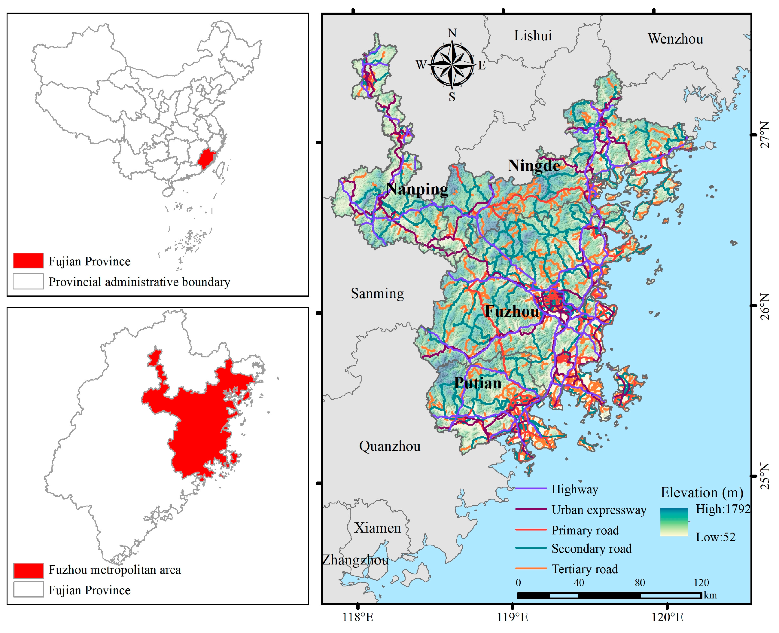
2.1. Study Area

The study area is defined by the “Fuzhou Metropolitan Area Development Plan (2021–2035)”, which includes the entire cities of Fuzhou and Putian, as well as parts of Ningde and Nanping, as depicted in Figure 1. The Fuzhou metropolitan area is situated on the southeastern coast of China and covers a land area of 26,000 km2, representing 21.5% of Fujian Province’s total area. The study area features a complex terrain of alternating plains and hills, characterized by a unique “mountain-sea-city-bay” pattern and urban landscape. However, the rapid advancement of urbanization, along with road expansions, has continuously degraded habitat quality and exerted sustained negative impacts on the ecological environment. By the end of 2022, the total road mileage had reached 46,900 km, with highway mileage increasing from 1267 km in 2014 to 2666 km in 2022, posing significant pressure on ecological environmental protection.

2.2. Data Sources and Pre-Processing
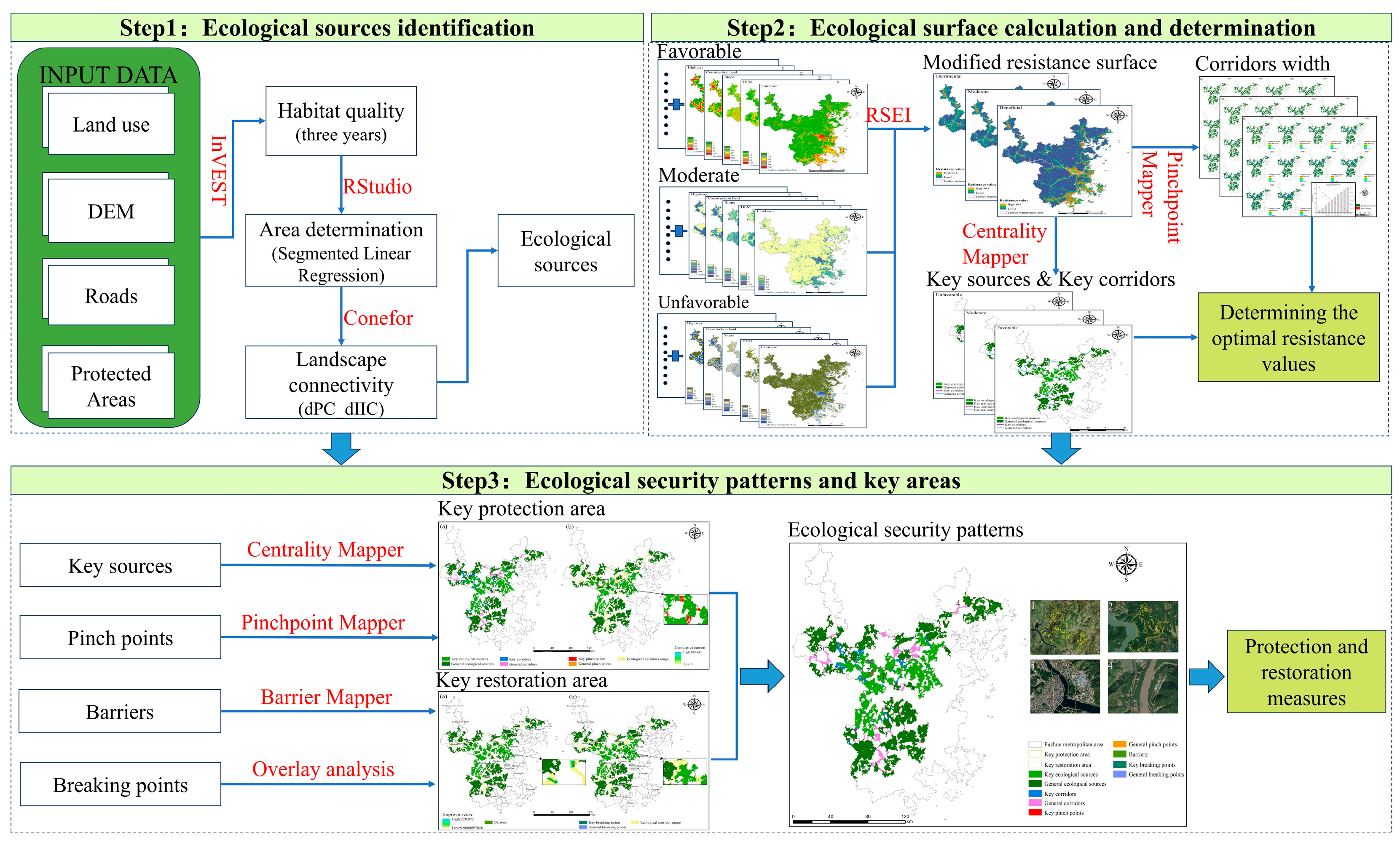
Table 1 presents the land-use data, factors threatening habitat quality, and factors for constructing resistance surfaces. The data primarily include land use, digital elevation model (DEM), and road network data. Land-use data are categorized into six types: forestland, cropland, grassland, water, unutilized land, and construction land. DEM data are utilized to derive elevation and slope information. The types of roads within the study area include highways, urban expressways, primary, secondary, and tertiary roads. To ensure spatial data consistency, all data have a resolution of 30 m × 30 m.

2.3. Methods

The framework of this study includes three main sections (Figure 2). Firstly, ecological sources are identified based on landscape connectivity and habitat quality. Secondly, resistance surfaces are constructed using resistance assignment methods categorized as favorable, moderate, and unfavorable, and these are modified using RSEI. The optimal resistance assignment method is then determined by analyzing key patches, key corridors, and the spatial extent of corridors. Thirdly, applying circuit theory to construct ESP identifies key ecological areas, and protection and restoration measures are proposed.

2.3.1. Identifying Ecological Sources

Ecological sources are regions characterized by high habitat quality and biodiversity, providing essential habitats for the survival and reproduction of species [28]. This study employs habitat quality evaluation, landscape connectivity analysis, and determination of patch area threshold to identify ecological sources.
This study employs the habitat quality module from the InVEST model for analysis [32]. High-quality habitats enhance species diversity and provide favorable living conditions. However, environmental changes and human disturbances lead to a severe decline in habitat quality. Therefore, this study classifies non-ecological land uses, including farmland, developed land, highways, urban expressways, and primary, secondary, and tertiary roads, as sources of threat. The parameters for calculating habitat quality were set based on existing research [33,34], and the data used in the InVEST model are presented in Table A1 and Table A2. The habitat quality was calculated for the years 2014, 2018, and 2022. Moreover, habitat quality was classified into five levels: bad (0–0.1), poor (0.1–0.3), fair (0.3–0.5), good (0.5–0.8), and excellent (0.8–1) [33]. Areas with consistently high habitat quality over the past eight years are designated as habitat stable areas.
Determining patch size is crucial for ensuring that ecological sources have sufficient ecological carrying capacity [35]. Larger patches provide more living space for species, while smaller patches can act as stepping stones to connect and support the ecological network [36]. Therefore, this study uses the segmented package in RStudio to perform segmented linear regression analysis on the total number of patches and their total area under different area thresholds.
Determining the distance threshold is a primary condition for calculating landscape connectivity [37]. The study uses the distance gradient method, evaluating the integral index of connectivity (IIC) and the number of components (NC) at distances of 100, 300, 500, 1000, 1500, 2500, 3500, 5000, 10,000, and 12,000 m, and standardizes the values. By analyzing the variations in the NC and IIC indices, the optimal distance threshold is determined and the probability of connectivity (PC) is evaluated. IIC and PC, as fundamental indices of landscape connectivity, are widely applied in overall landscape connectivity assessments [38,39]. However, considering the importance of various landscape component, this study employs the delta integration index of connectivity (dIIC) and the delta probability of connectivity (dPC) to assess the connectivity of local landscapes [40]. By fitting dIIC and dPC, the dPC_IIC index is obtained, with habitat stability areas where dPC_IIC > 1 are selected as ecological sources. The calculation formulas are shown in Table 2.

2.3.2. Constructing Resistance Surfaces Based on Different Resistance Assignment Methods

Resistance surface represents the level of resistance that species must overcome when moving through different landscape units. When constructing resistance surfaces, most studies have adopted a single subjective assignment method for resistance factors [41,42]. It lacks exploration of the impacts of various assignment methods on ESP. Therefore, this study proposes different resistance assignment methods categorized as favorable, moderate, and unfavorable (Table 3). Additionally, the impact of roads on ecosystems generally varies across different road grades, making it inappropriate to assign a uniform weight to all roads. Therefore, principal component analysis is employed to calculate the weights of resistance factors such as land use, slope, elevation, distance to construction land, and distance to roads of different grades. The weights of different resistance factors are determined through principal component analysis, and the basic resistance surface is modified using the RSEI [43]. The RSEI data was calculated through the Google Earth Engine platform. The formula for modifying the resistance surface as follows:
R m o d i f i e d = R i n i t i a l × 1 R S E I n o r m
where Rmodified represents the modified resistance surface; Rinitial represents the initial resistance surface; and RSEInorm represents the normalized RSEI. The larger RSEInorm value, the smaller Rmodified, indicating that areas with better ecological quality have lower resistance.

2.3.3. Extracting Ecological Corridors

Ecological corridors are linear areas that link different source areas and facilitate ecological processes among species [44]. Circuit theory employs fundamental electrical principles to model the movement of species within a landscape [45]. This model interprets current as the capacity of species to move within the ecological network. Higher current indicates lower resistance, thereby increasing the possibility of species traversing the area [44]. The Linkage Pathways module is employed to identify ecological corridors, allowing for the determination of multiple routes through which species can traverse source areas. The lowest-cost path is defined as the optimal ecological corridor, with its width determined by the cumulative resistance threshold [28,46].

2.3.4. Evaluating Importance of Ecological Sources and Corridors

Centrality Mapper determines the importance of ecological sources and corridors by simulating the distribution of current within the network [47]. Specifically, 1 ampere is input into one ecological source while another source is grounded. By summing the currents flowing through all ecological sources and corridors, centrality scores are calculated. Areas with higher scores indicate greater importance and connectivity within the ecological network. The lowest-cost path is defined as the optimal ecological corridor, with its width determined by the cumulative resistance threshold [28,46].

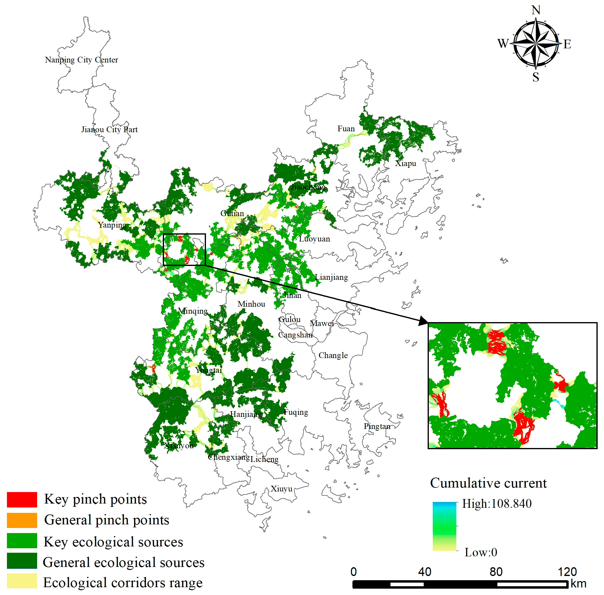
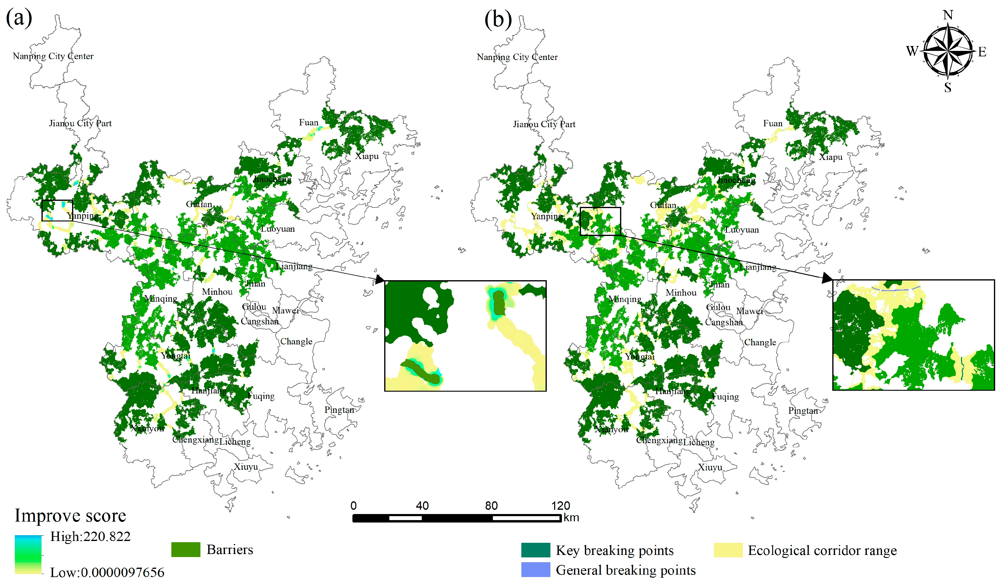
2.3.5. Identifying Ecological Nodes

The width of corridors directly influences its ecological function and defines its role within the ecological network. This width is determined by the cumulative resistance threshold from circuit theory [48]. For different resistance assignment methods, the cumulative resistance threshold is set from 500 to 5000 in increments of 500. By analyzing the proportion of ecological land including forest land, grassland, and water within the corridors under different thresholds, the optimal resistance assignment method is determined.
Pinch point, also known as a bottleneck, is an area within the ecological network where the current density is high and species frequently migrate. Focusing on the safeguarding of these areas not only improves the accessibility of ecological sources but also reduces the ecological risk of the entire region [49]. Pinchpoint Mapper is used to identify pinch points within ecological corridors, and areas with heighten current density on key corridors are designated as key pinch points.
Barrier is an area that obstructs species migration. Restoring these areas can reduce ecological risks and enhance species migration [50]. Using Barrier Mapper, the search radius is defined with a minimum of 100 m and a maximum of 500 m, with a step size of 100 m, to detect barriers and calculate improvement scores. Improvement scores are used to assess and prioritize obstacles within the ecological network; higher improvement scores indicate a greater likelihood of functioning as obstacles.
Breaking point is a gap in the continuity of an ecological corridor, such as where roads cut through ecological corridors, creating a barrier effect that hinders species movement between ecological sources on either side of the road [51]. The intersections of ecological corridors with major traffic roads (highways, urban expressways) are considered breaking points. Breaking points that coincide with pinch points and barriers are regarded as key breaking points.

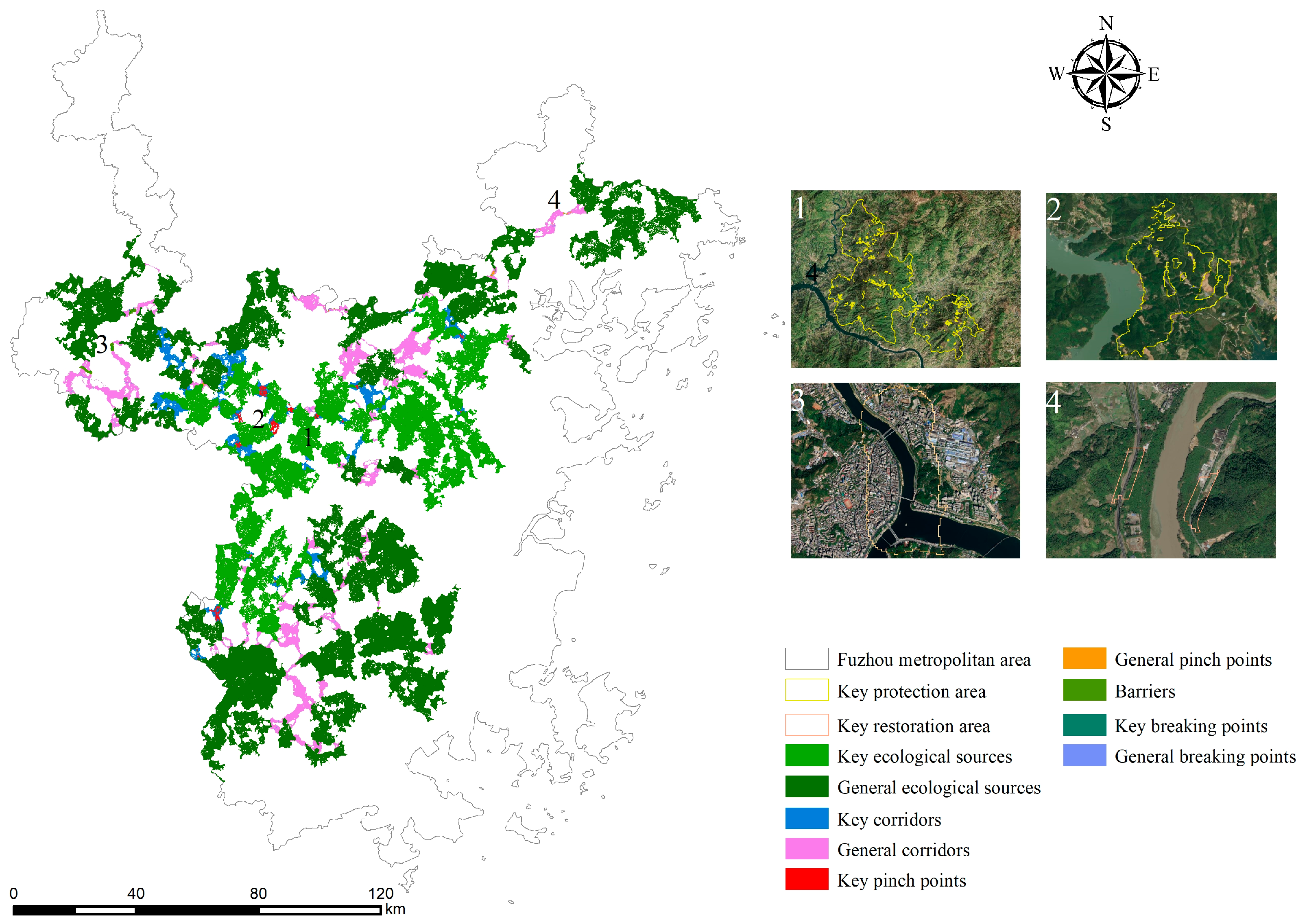
2.3.6. Determining Critical Ecological Areas for Protection and Restoration

Critical ecological protection areas possess significant ecological functions and high ecological value, serving as vital habitats for species. These areas play a vital role in sustaining ecological balance and enhancing overall ecological health [52]. In contrast, critical ecological restoration areas are regions where landscape connectivity is obstructed, making it difficult for species to traverse. These areas have high ecological restoration potential and can significantly enhance ecosystem functions and biodiversity after restoration [46]. This study identifies key patches and ecological pinch points as essential areas for conservation, while barriers and key breaking points are identified as critical areas for ecological restoration.

3. Results

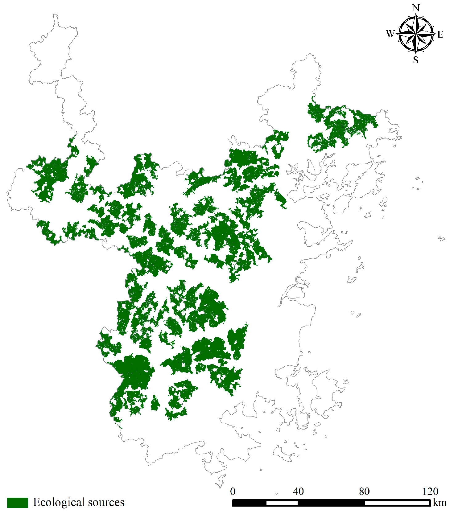
3.1. Spatial Distribution of Ecological Sources

3.1.1. Assessment of Habitat Quality

From 2014 to 2022, areas with high habitat quality in the Fuzhou metropolitan area were widely distributed, avoiding many urban built-up areas and cropland (Figure 3). The area of regions with high habitat quality reduced from 12,746.35 km2 to 9312.33 km2, with their percentage in the study area declining from 47.34% to 34.59%. By overlaying the high habitat quality zones from the three periods, habitat stable areas were identified (Figure 3d). The habitat stable areas cover 9044.77 km2, accounting for 33.59% of the study area. The building of numerous roads within the study area caused a significant decline in habitat quality. Policies that convert cropland to forests and grasslands, as well as restrict large-scale urban development, enhance habitat quality.

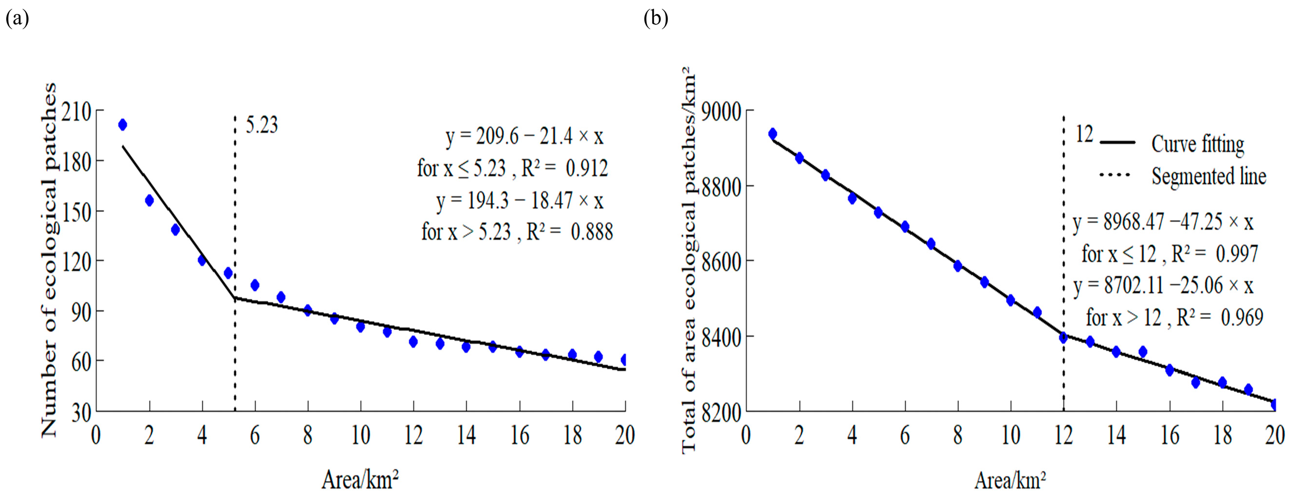
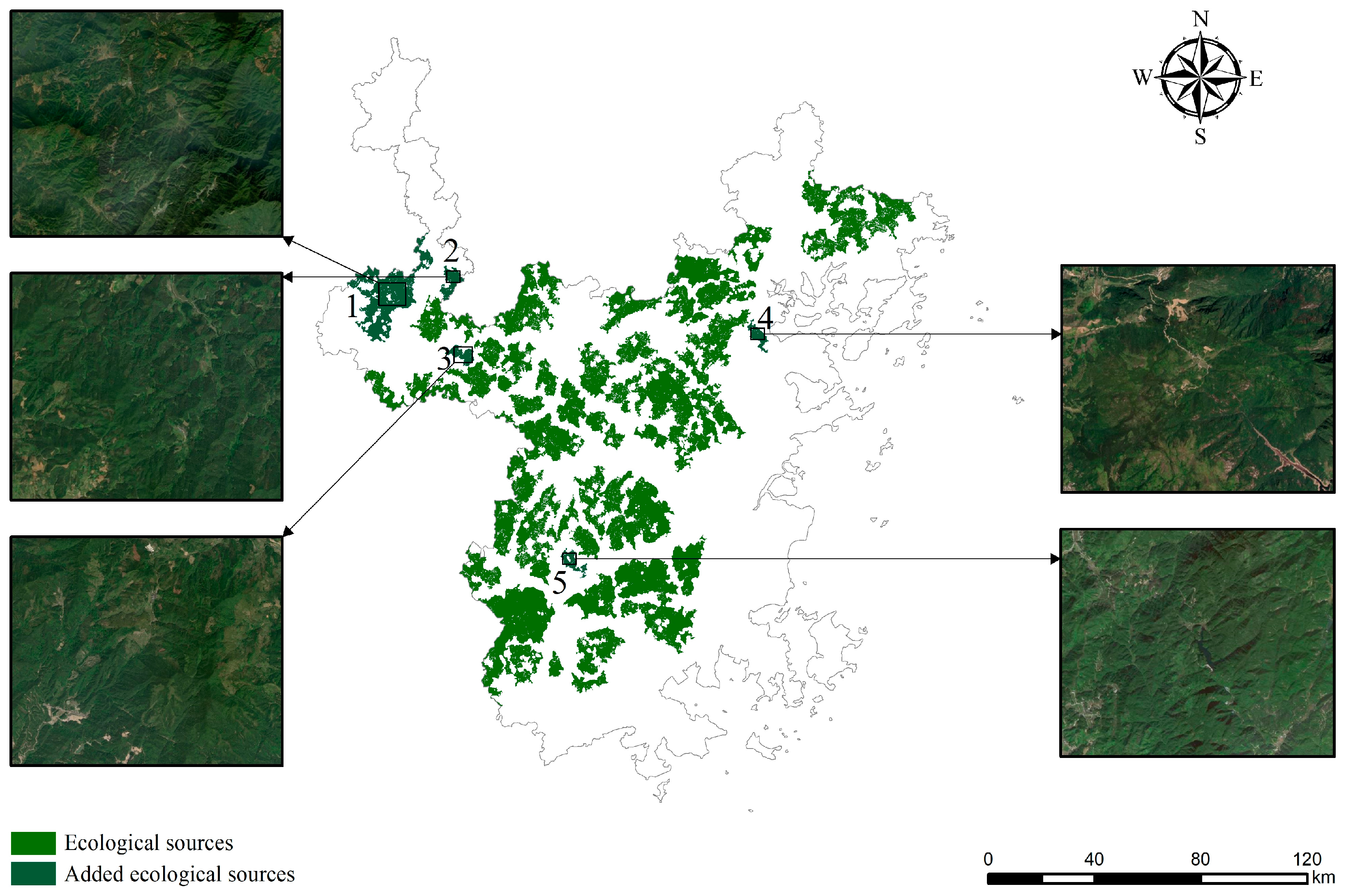
3.1.2. Identification and Analysis of Ecological Sources

A total of 201 patches larger than 1 km2 were identified in habitat stable areas. As the patch area threshold within the habitat stable areas increases from 1 km2 to 20 km2, the quantity of patches descends from 201 to 60, and the total area decreases from 8935.9 km2 to 8216.9 km2 (Figure 4). When the patch area threshold is less than 5.23 km2, the number of patches changes significantly, indicating the presence of many fragmented small patches. To avoid overestimating the ecological benefits of small patches, the optimal area threshold should be greater than 5.23 km2 (Figure 4a). When the patch area threshold exceeds 12 km2, the total patch area tends to stabilize, indicating that only large patches are included. To ensure small patches, which serve as stepping stones in the overall landscape, are not overlooked, the optimal area threshold should be less than 12 km2 (Figure 4b). Meanwhile, to ensure the identified ecological sources provide sufficient ecological carrying capacity, this study selects 10 km2 as the optimal patch area threshold.
To enhance the accuracy of landscape connectivity calculations, the optimal distance threshold is determined based on the changes in NC and IIC indices under different distance thresholds (Figure 5). The distance threshold is positively associated with the IIC index and negatively associated with the NC index. This indicates that with an increasing distance threshold, landscape connectivity improves significantly, offering species more migration pathways and habitat options. When the distance threshold falls below 3500 m, the NC index experiences a significant decrease, while the IIC and Sum indices increase rapidly. Beyond 3500 m, the changes in the IIC, NC, and Sum indices gradually level off. Thus, the ideal distance threshold for assessing the landscape connectivity of ecological sources is 3500 m.
At a 10 km2 area threshold and a 3500 m distance threshold, 41 ecological sources with high habitat quality and connectivity are identified through dPC_IIC > 1 calculations (Figure 6). The combined area of these ecological sources is 7218.21 km2, representing 26.81% of the total study area. The main land-use type for ecological sources is forest, which is primarily situated in the central, northern, and southwestern regions of the study area. However, the coastal areas of the study region are severely lacking in ecological sources due to rapid urbanization.

3.2. Comparison of Ecological Corridors with Different Resistance Assignment Methods

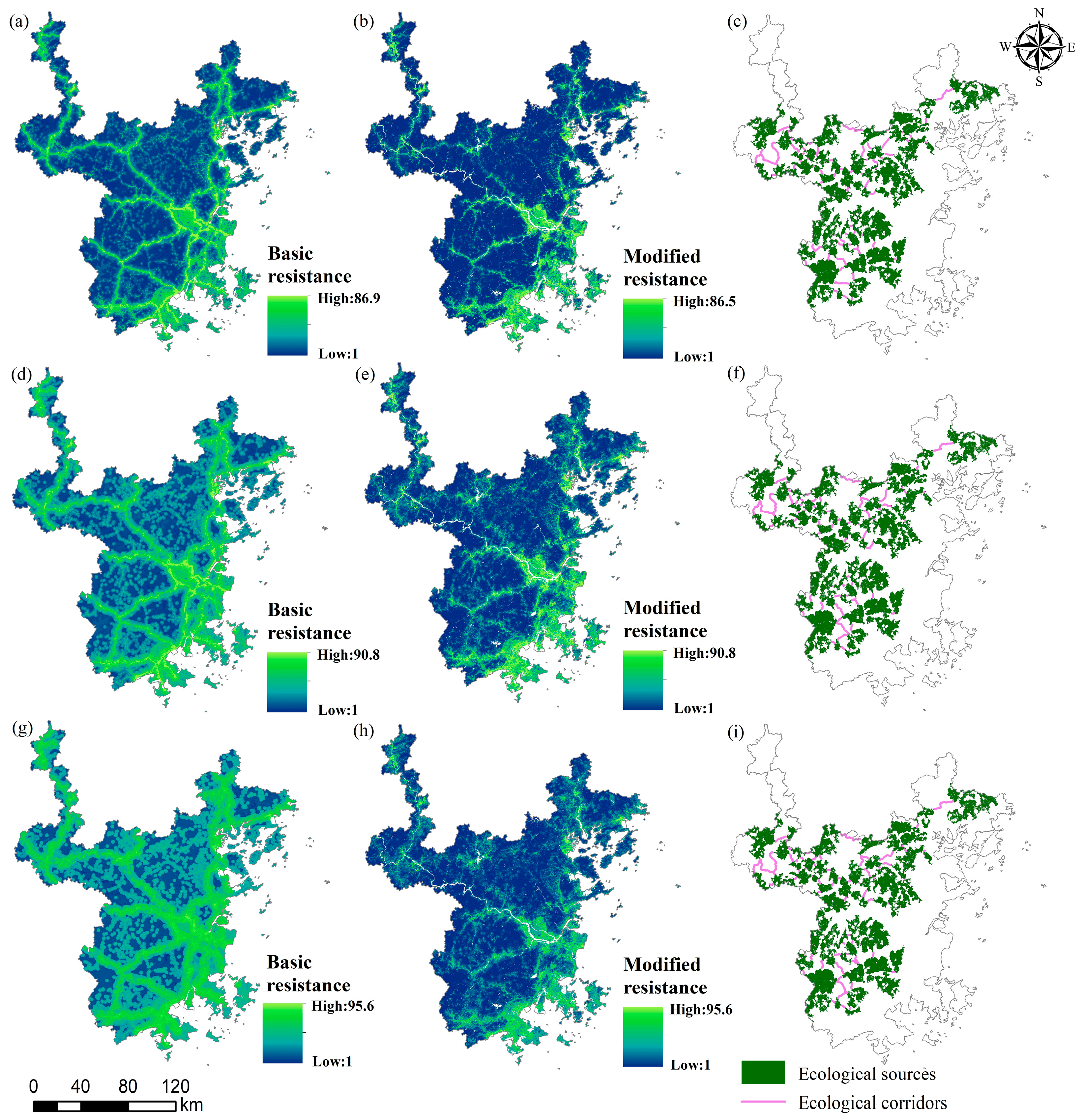
3.2.1. Spatial Distribution of Resistance Surfaces and Corridors

The fundamental resistance surfaces constructed using favorable, moderate, and unfavorable methods have average resistance values of 17.3, 27.44, and 37.75, respectively. However, the low-resistance areas are discontinuous and severely fragmented, and the boundaries of the high-resistance areas significantly differ from the actual situation (Figure 7a,d,g). This discrepancy is due to the overestimation of the impact of human disturbances on the resistance surface. Compared to the fundamental resistance surfaces, the resistance surfaces modified by RSEI are more detailed (Figure 7b,e,h). Specifically, under the favorable method, low-resistance areas exhibit good continuity, while under the moderate and unfavorable methods, the low-resistance areas become notably fragmented and the range of high-resistance areas rises. Furthermore, regardless of the resistance assignment method, the overall resistance values show a decreasing trend from the southern and southeastern parts to the northwestern part of the study area. High-resistance values are primarily situated in the southern and southeastern urban areas with intensive human activities, forming strip and patch distributions. In contrast, low-resistance values are primarily located in forest-dominated and hilly areas, forming patch distributions.
Ecological corridors, under various resistance assignment methods, display a spatial pattern with high density in the southwestern and northern regions and sparsity in the central area (Figure 7e,f,i). However, the identified ecological corridors exhibit differences. Specifically, under the favorable, moderate, and unfavorable valuation methods, a total of 73, 71, and 70 ecological corridors were extracted, having total lengths of 338.15 km, 361.76 km, and 363.81 km, and average lengths of 4.63 km, 5.1 km, and 5.2 km, respectively. Additionally, the total cost-weighted distances of the ecological corridors are 9.49 × 10⁵, 1.39 × 10⁶, and 1.83 × 10⁶, respectively. This indicates that ecological corridors under different resistance assignment methods show considerable deviation, requiring certain curvature to connect ecological sources.

3.2.2. Optimal Resistance Assignment Method Determination

Under different resistance assignment methods, the number of key patches identified through current centrality analysis remains consistent, totaling 13. These patches cover a combined area of 2435.44 km2, accounting for 33.74% of the total area of ecological sources, and are solely located in the central region (Figure 8a–c). This indicates that different resistance assignment methods do not alter the spatial location of key patches. However, the identification of key corridors shows significant differences. Specifically, compared to the favorable and unfavorable methods, the moderate resistance assignment method identifies the greatest number of key corridors, totaling 26 with a combined length of 41.29 km (Figure 8b). Additionally, under this method, key corridors are distributed throughout the network, connecting numerous key patches. This broadens the radiation range of high-quality ecological spaces provided by key patches.
Under various resistance assignment methods, the area of ecological corridors increases as the cumulative resistance threshold rises, while the proportion of ecological land within these corridors consistently decreases (Figure 9). Specifically, as the cumulative resistance threshold increases from 500 to 5000, under the favorable method, the area of ecological corridors expands from 286.92 km2 to 2687.77 km2, with a large expansion concentrated in the southwestern and northern regions. The percentage of ecological land decreases from 97.20% to 91.57% (Figure 9a). While wider ecological corridors have significant ecological effects, they also result in land resource waste, fragmented surrounding habitats, and reduced overall efficiency of ecological protection efforts. Under the unfavorable method, the area of ecological corridors increases from 132.94 km2 to 979 km2, but the limited expansion leads to lower corridor stability, with the percentage of ecological land dropping from 98.59% to 95.46% (Figure 9c). Extremely narrow ecological corridors experience strong edge effects, making them insufficient to support the rapid material cycling and energy flow required by ecosystems. Compared to the other two methods, the moderate method increases the area of ecological corridors from 171.36 km2 to 1439.24 km2, with a more balanced area expansion, primarily concentrated in the southern, northern, and southeastern parts of the study area. This method maximizes ecological function, with the percentage of ecological land decreasing from 98.09% to 94.44%, ensuring sufficient biological carrying capacity without significantly increasing the cost of ecological protection due to overly wide corridors (Figure 9b). Therefore, this study identifies the moderate method as the optimal resistance assignment method. Additionally, under the moderate method, the area of ecological corridors shows a significant increasing trend (Figure 10a), while the average current value shows a significant decreasing trend (Figure 10b). It is noteworthy that when the cumulative resistance threshold reaches 3500, both the corridor area increase trend and the average current value decrease trend change significantly. This indicates that when the cumulative resistance threshold exceeds 3500, greater resistance must be overcome to increase the width of the corridor. However, overly wide corridors result in current dispersion, increasing species migration time and corridor construction costs. Therefore, this study adopts a threshold of 3500 to define the width of the corridors.

3.3. Spatial Analysis for Key Ecological Areas

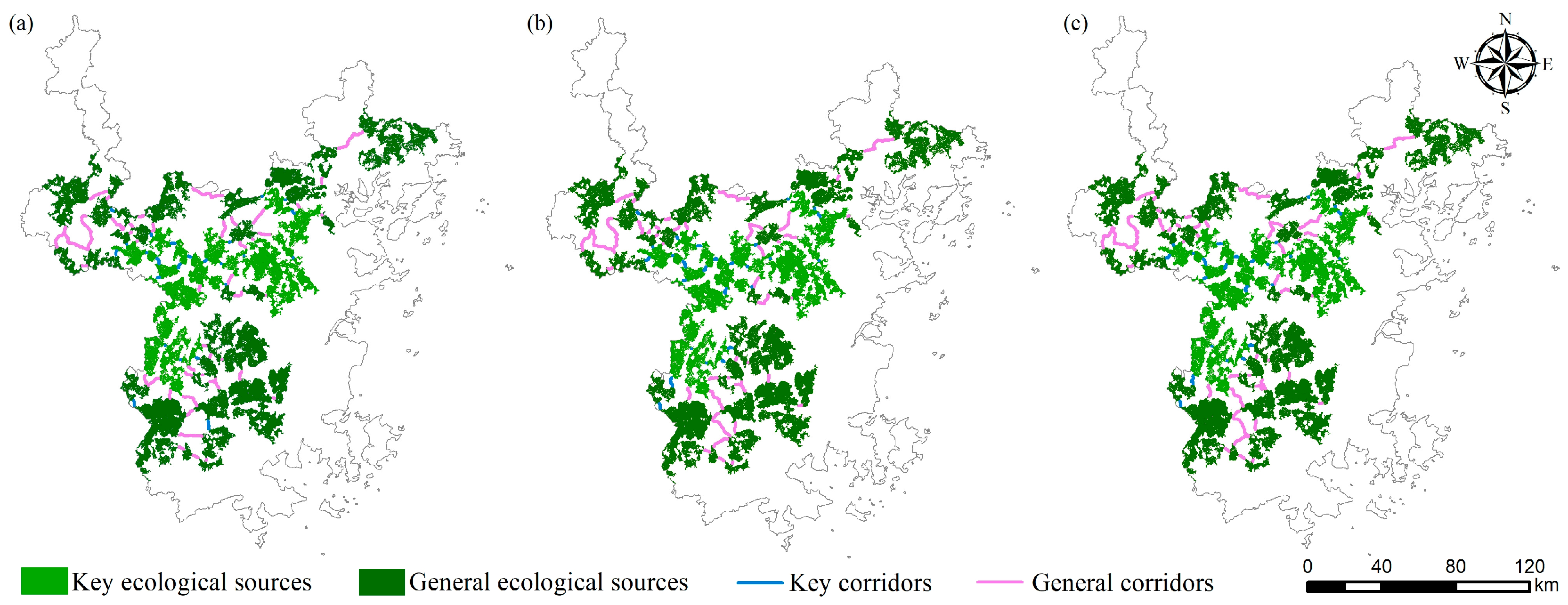
3.3.1. Spatial Distribution of Critical Areas for Protection

When the cumulative resistance threshold is set at 3500, areas with high cumulative current intensity are identified as pinch points (Figure 11). Seventy-two pinch points are identified within the study area, covering the area of 41.37 km2. The primary land-use types of these pinch points are cropland and forest. Spatially, the distribution of pinch points increases gradually from the south to the north of the study area. Among these, 26 are identified as key pinch points, covering the area of 34.35 km2, which represents 83.03% of the total pinch point area. These key pinch points are mainly located at the junction of Yanping District, Gutian, and Minhou, connecting most of the key patches. Key pinch points play a significant role in improving habitat quality and maintaining biodiversity. The loss of function at key nodes can lead to widespread landscape fragmentation, severely impacting species survival. General pinch points serve a limited range of species and are more dispersed, with relatively small areas, and their contribution to resource exchange between ecological sources is limited. Therefore, prioritizing the protection of key pinch points can greatly enhance landscape connectivity.

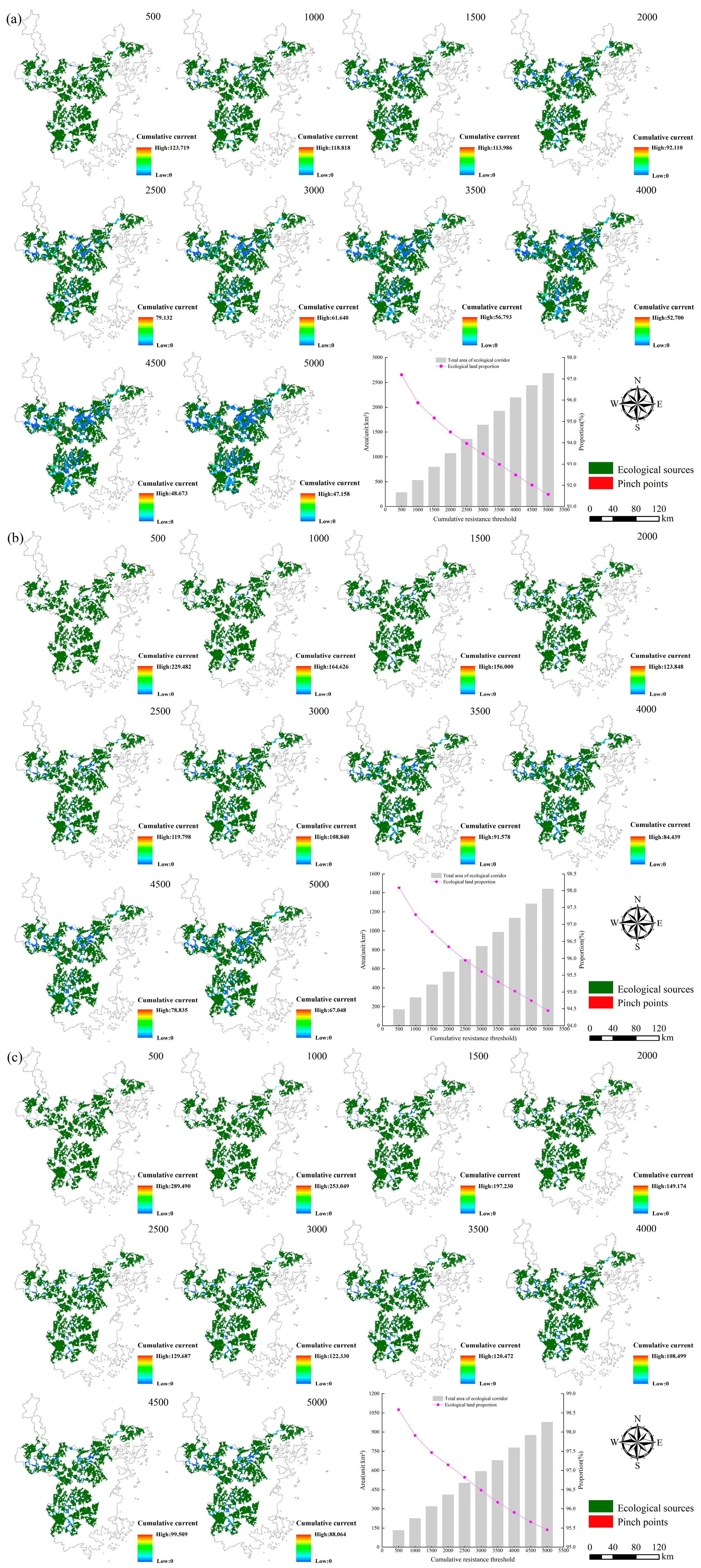
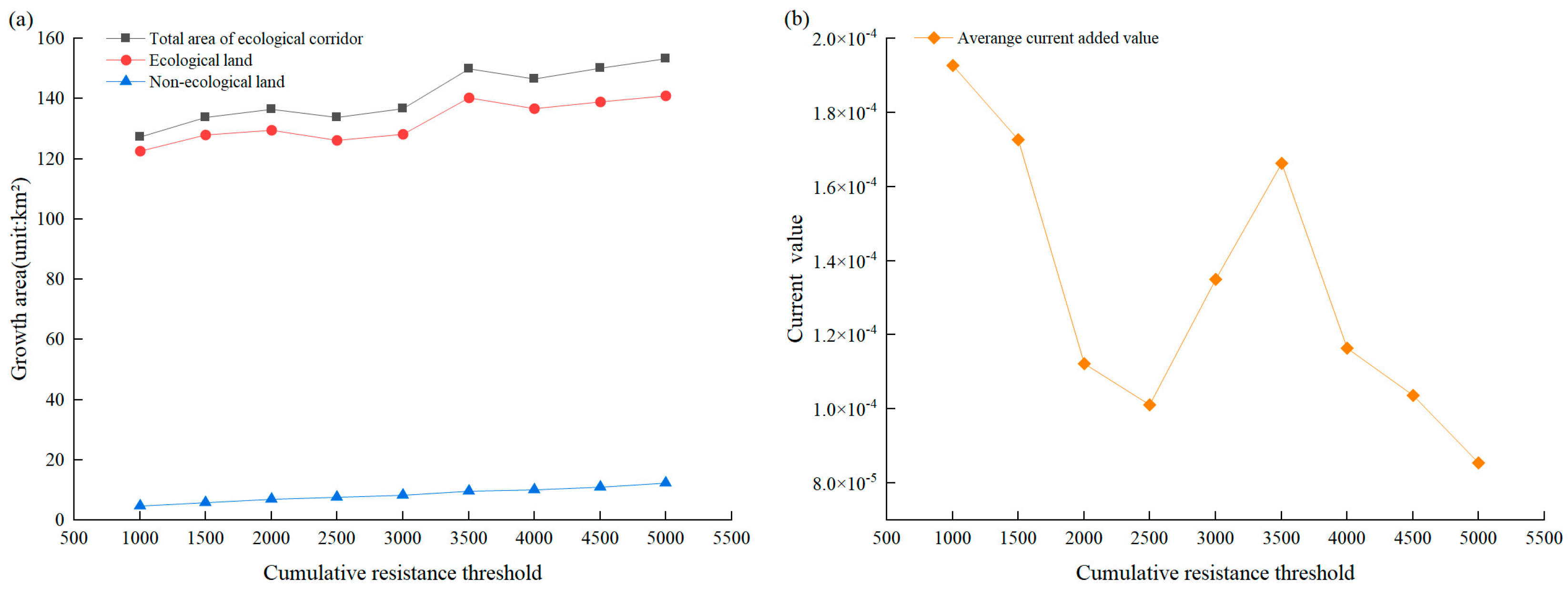
3.3.2. Spatial Distribution of Critical Areas for Restoration

This study designates barriers and key breaking points as critical areas for ecological restoration. The study area includes a total of 7 barriers and 47 breaking points, covering areas of 10.71 km2 and 12.14 km2, respectively. The land-use types of barriers are predominantly construction land and cropland, primarily located in Yanping District, while the land-use types of breaking points are mainly forestland and cropland (Figure 12a). Among these, 21 key breaking points are identified, with 8 intersecting highways and 13 intersecting urban expressways, covering the area of 3.84 km2, which constitutes 31.63% of the total area. These key breaking points are primarily concentrated in Yanping District, Gutian, and Yongtai, where habitat quality is relatively high (Figure 12b). Due to the significant overlap of these key breaking points with pinch points and barriers, they create a pronounced cutting effect on corridors, hindering connectivity and exacerbating landscape fragmentation.

4. Discussion

4.1. Effectiveness of Ecological Sources Identification

Ecological sources are fundamental to ESP [53]. From the view of ecological processes and functions, graph-theory-based connectivity models are widely used for identifying ecological sources, among which the dPC and dIIC indices are the most commonly used to measure the connectivity of individual patches [54]. However, existing studies often use these two indices separately, lacking comprehensive consideration of the insensitivity of the dPC index to neighboring patches and the sensitivity of the dIIC index to the distances between patches [38]. Thus, this study fits the dPC and dIIC indices to obtain the composite index dPC_IIC (Equation (7)) and further determines the validity of this index (Figure 13). When selecting dPC > 1, sources 1 and 2, covering a combined area of 419.6 km2, are not identified as ecological sources. Similarly, when selecting dIIC > 1, sources 3, 4, and 5, with a total area of 111.03 km2, are also excluded as ecological sources. Based on satellite images, individual validation of sources 1–5 reveals that they have high habitat quality and large forest cover, providing a foundation for being considered ecological sources. This indicates that the newly fitted index dPC_IIC is more scientific and accurate for identifying ecological sources, thus further protecting areas of high habitat quality against the pressures of urban development.

4.2. Variations in Resistance Surfaces and Corridors Resulting from Different Resistance Assignment Methods

Resistance surfaces are a critical step in developing a scientific ESP, as they enable more accurate identification of ecological protection and restoration areas, facilitating the evaluation of overall ecosystem stability and connectivity [44]. In existing studies, some scholars have constructed resistance surfaces using methods such as habitat quality-based models, entropy coefficient methods, and expert scoring techniques [37]. Other scholars have modified resistance surfaces by incorporating factors like nighttime lighting and land growth probability [55].These studies aim to ensure that the constructed resistance surfaces accurately reflect the difficulty of species migration. However, they overlook the potential impact of different resistance assignment methods on both the resistance surface and ecological corridors. Therefore, this study classifies resistance assignment into three methods: favorable, moderate, and unfavorable, and constructs resistance surfaces accordingly. It uses the RSEI to modify the resistance surfaces to objectively represent the ecological quality (Figure 7). Finally, circuit theory is employed to calculate the current density of ecological corridors within the same cumulative resistance threshold range (Figure 9). The results show that the resistance surfaces modified by RSEI have average resistance values of 8.1, 11.32, and 14.7. These resistance surfaces accurately reflect the actual natural conditions of the surface (Figure 7b,e,h), indicating the trend of ecological quality changes to some extent, while also reducing the subjective influence of empirical resistance value assignments. Additionally, this study finds that different resistance assignment approaches significantly affect the spatial location and width of corridors. Specifically, the cumulative resistance threshold increases from 500 to 5000, the corridor area calculated using the favorable approach accounts for 1.07%, 1.98%, 2.97%, 4.00%, 5.05%, 6.13%, 7.15%, 8.16%, 9.09%, and 9.98% of the total study area (Figure 9a); the moderate approach accounts for 0.64%, 1.11%, 1.61%, 2.11%, 2.61%, 3.12%, 3.67%, 4.22%, 4.78%, and 5.35% (Figure 9b); and the unfavorable approach accounts for 0.49%, 0.84%, 1.18%, 1.53%, 1.87%, 2.20%, 2.53%, 2.89%, 3.26%, and 3.64% (Figure 9c). The corridor area shows a significant positive correlation with the cumulative resistance threshold. However, under favorable conditions, corridor areas expand most rapidly. While wide corridors provide species with more habitat space, they also increase predation risks and hinder urban development. Under the unfavorable approach, the corridor area grows the slowest, and narrow corridors are not conducive to species’ ecological behaviors and have strong edge effects. Therefore, compared to the favorable and unfavorable approaches, the moderate approach strikes a balance between realizing ecological benefits and meeting the demands of economic development.

4.3. Implications and Limitations

This study seeks to enhance the accuracy of ESP construction by identifying the optimal resistance assignment method, which in turn allows for the determination of key areas within the study region that require protection and restoration (Figure 14). The key ecological protection areas in the study region cover a total of 2469.79 km2, including 2435.44 km2 of key patches and 34.35 km2 of key pinch points. The key ecological restoration areas in the study region cover a total of 14.55 km2, including 10.71 km2 of barriers and 3.84 km2 of key breaking points. Overall, the key ecological protection areas are extensive and significantly contribute to landscape connectivity. The key ecological restoration areas are smaller and more dispersed within the study area, but restoring these areas is beneficial for maintaining or enhancing the integrity of ecological functions. Therefore, based on Google Earth satellite images, four key ecological areas were chosen for validation, and relating measures were suggested (Table 4).
However, there are a few constraints in this research. Firstly, this study determines the optimal resistance assignment method based on corridor width, but there is still no consensus on the index selection and methodology for determining corridor width [56,57,58]. Secondly, the selection of resistance factors is extensive, and this study only selects land type, DEM, slope, distance to construction land, and distance to roads of different grades as resistance factors for constructing the resistance surface, which may not fully reflect the actual natural ecological conditions of the study area. The construction of resistance surfaces from a static view lacks in-depth discussion on ecological processes and species movement behaviors [59]. Additionally, this study lacks a detailed quantification of the impact of different resistance assignment methods on ecosystem functions from an ecosystem services perspective. Therefore, future research should strengthen data collection and sharing mechanisms, further investigating corridor width from the perspectives of corridor structure and functional composition. Furthermore, a dynamic approach and ecosystem services calculations should be adopted to better understand various ecological processes within ecosystems and to quantify ecosystem functions.

5. Conclusions

This study addresses the lack of exploration on the impact of resistance value assignment on resistance surface construction by proposing three resistance assignment methods. By identifying the optimal resistance assignment method, a framework is established for the protection and restoration of key areas. This framework helps reduce subjectivity in resistance surface construction and improves the accuracy of constructing ESP. The results show the following:
(1) The moderate method is the optimal resistance assignment. Under this method, the area of ecological corridors ranges from 171.36 to 1439.24 km2. When the cumulative resistance threshold is 3500, the corridor area is 989.17 km2, with ecological land accounting for 95.30%, effectively meeting the needs of species migration, gene flow, and material cycling.
(2) Different resistance assignment methods do not change the spatial distribution of key patches, but the identification of key corridors shows significant spatial heterogeneity. Notably, under the moderate resistance assignment method, the identified key corridors exhibit the widest distribution, primarily radiating outward from the center of the study area and effectively connecting most key patches.
(3) The study identifies 41 ecological sources, encompassing a combined area of 7218.21 km2. Using the moderate resistance assignment method, key areas for ecological protection and restoration are identified as 2469.79 km2 and 14.55 km2, respectively. This includes 13 key patches, 26 key pinch points, 7 barriers, and 21 key breaking points. In the context of limited economic resources, conserving and restoring these areas helps achieve the sustainable development goal of minimizing costs while maximizing ecological benefits.

Author Contributions

Conceptualization, X.H.; methodology, X.H.; software, D.J.; writing—original draft preparation, D.J.; writing—review and editing, X.H.; data curation, W.Q. and R.G.; visualization, M.W. and Z.W.; supervision, X.H. All authors have read and agreed to the published version of the manuscript.

Funding

This research was funded by the National Natural Science Foundation of China (31971639), the Natural Science Foundation of Fujian Province (2023J01477), and the Special Fund Project for Scientific and Technological Innovation of Fujian Agriculture and Forestry University (KFB24049).

Data Availability Statement

The raw data supporting the conclusions of this article will be made available by the authors on request.

Acknowledgments

The authors would like to thank the Faculty of the College of Transportation and Civil Engineering, Fujian Agriculture and Forestry University.

Conflicts of Interest

The authors declare no conflicts of interest.

Appendix A

Table A1. Threat factor parameters.
Threat FactorMAX_DIST (km)WeightDistance—Decay Function
Cropland10.6linear
Construction land61linear
Highways50.6exponential
Urban expressways40.5exponential
Primary roads30.4exponential
Secondary roads20.3exponential
Tertiary roads10.2exponential
Table A2. Sensitivity parameters of different land-use types to habitat threat factors.
Habitat TypeHabitat SuitabilityCroplandConstruction LandHighwaysUrban ExpresswaysPrimary RoadsSecondary RoadsTertiary Roads
Cropland0.600.80.70.60.60.50.4
Forestland10.60.90.80.70.70.60.5
Grassland0.80.30.80.80.70.70.50.4
water0.90.40.60.60.50.40.40.3
Unutilized land0.30.10.30.50.30.20.20.1
Construction land0000.30.20.20.10.1

References

  1. Wei, L.; Zhou, L.; Sun, D.; Yuan, B.; Hu, F. Evaluating the impact of urban expansion on the habitat quality and constructing ecological security patterns: A case study of Jiziwan in the Yellow River Basin, China. Ecol. Indic. 2022, 145, 109544. [Google Scholar] [CrossRef]
  2. Kubacka, M.; Żywica, P.; Subirós, J.V.; Bródka, S.; Macias, A. How do the surrounding areas of national parks work in the context of landscape fragmentation? A case study of 159 protected areas selected in 11 EU countries. Land Use Policy 2022, 113, 105910. [Google Scholar] [CrossRef]
  3. Wang, R.; Zhu, Q.-C.; Zhang, Y.-Y.; Chen, X.-Y. Biodiversity at disequilibrium: Updating conservation strategies in cities. Trends Ecol. Evol. 2022, 37, 193–196. [Google Scholar] [CrossRef] [PubMed]
  4. Yao, S.; Li, Y.; Quan, X.; Xu, J. Applying the driver-pressure-state-impact-response model to ecological restoration: A case study of comprehensive zoning and benefit assessment in Zhejiang Province, China. Glob. Ecol. Conserv. 2024, 55, e03222. [Google Scholar] [CrossRef]
  5. Yu, K. Security patterns and surface model in landscape ecological planning. Landsc. Urban Plan. 1996, 36, 1–17. [Google Scholar] [CrossRef]
  6. Peng, J.; Liu, Y.; Corstanje, R.; Meersmans, J. Promoting sustainable landscape pattern for landscape sustainability. Landsc. Ecol. 2021, 36, 1839–1844. [Google Scholar] [CrossRef]
  7. Peng, J.; Xu, D.; Xu, Z.; Tang, H.; Jiang, H.; Dong, J.; Liu, Y. Ten key issues for ecological restoration of territorial space. Natl. Sci. Rev. 2024, 11, nwae176. [Google Scholar] [CrossRef]
  8. Fan, J. Theoretical innovation in optimization of protection and development of China’s territorial space and coping strategy of 13th Five-Year Plan. Bull. Chin. Acad. Sci 2016, 31. [Google Scholar] [CrossRef]
  9. Huang, L.; Wang, J.; Fang, Y.; Zhai, T.; Cheng, H. An integrated approach towards spatial identification of restored and conserved priority areas of ecological network for implementation planning in metropolitan region. Sustain. Cities Soc. 2021, 69, 102865. [Google Scholar] [CrossRef]
  10. Hou, W.; Zhai, L.; Walz, U. Identification of spatial conservation and restoration priorities for ecological networks planning in a highly urbanized region: A case study in Beijing-Tianjin-Hebei, China. Ecol. Eng. 2023, 187, 106859. [Google Scholar] [CrossRef]
  11. Gao, C.; Pan, H.; Wang, M.; Zhang, T.; He, Y.; Cheng, J.; Yao, C. Identifying priority areas for ecological conservation and restoration based on circuit theory and dynamic weighted complex network: A case study of the Sichuan Basin. Ecol. Indic. 2023, 155, 111064. [Google Scholar] [CrossRef]
  12. Gao, M.; Hu, Y.; Bai, Y. Construction of ecological security pattern in national land space from the perspective of the community of life in mountain, water, forest, field, lake and grass: A case study in Guangxi Hechi, China. Ecol. Indic. 2022, 139, 108867. [Google Scholar] [CrossRef]
  13. Weber, T.; Sloan, A.; Wolf, J. Maryland’s Green Infrastructure Assessment: Development of a comprehensive approach to land conservation. Landsc. Urban Plan. 2006, 77, 94–110. [Google Scholar] [CrossRef]
  14. Aminzadeh, B.; Khansefid, M. A case study of urban ecological networks and a sustainable city: Tehran’s metropolitan area. Urban Ecosyst. 2010, 13, 23–36. [Google Scholar] [CrossRef]
  15. Kong, F.; Yin, H.; Nakagoshi, N.; Zong, Y. Urban green space network development for biodiversity conservation: Identification based on graph theory and gravity modeling. Landsc. Urban Plan. 2010, 95, 16–27. [Google Scholar] [CrossRef]
  16. Wang, C.; Yu, C.; Chen, T.; Feng, Z.; Hu, Y.; Wu, K. Can the establishment of ecological security patterns improve ecological protection? An example of Nanchang, China. Sci. Total Environ. 2020, 740, 140051. [Google Scholar] [CrossRef] [PubMed]
  17. Regolin, A.L.; Oliveira-Santos, L.G.; Ribeiro, M.C.; Bailey, L.L. Habitat quality, not habitat amount, drives mammalian habitat use in the Brazilian Pantanal. Landsc. Ecol. 2021, 36, 2519–2533. [Google Scholar] [CrossRef]
  18. Liu, Y.; Huang, X.; Li, J.; Wang, Z.; Xu, C.; Xu, Y. Ecological connectivity analysis of typical coastal areas in China: The case of Zhangzhou City, Fujian Province. Urban Clim. 2024, 53, 101826. [Google Scholar] [CrossRef]
  19. Jiang, H.; Peng, J.; Dong, J.; Zhang, Z.; Xu, Z.; Meersmans, J. Linking ecological background and demand to identify ecological security patterns across the Guangdong-Hong Kong-Macao Greater Bay Area in China. Landsc. Ecol. 2021, 36, 2135–2150. [Google Scholar] [CrossRef]
  20. Lu, Y.; Huang, D.; Tong, Z.; Liu, Y.; He, J.; Liu, Y. A conceptual framework for constructing and evaluating directed ecological networks: Evidence from Wuhan Metropolitan Area, China. Environ. Impact Assess. Rev. 2024, 106, 107464. [Google Scholar] [CrossRef]
  21. Stevens, V.M.; Polus, E.; Wesselingh, R.A.; Schtickzelle, N.; Baguette, M. Quantifying functional connectivity: Experimental evidence for patch-specific resistance in the Natterjack toad (Bufo calamita). Landsc. Ecol. 2004, 19, 829–842. [Google Scholar] [CrossRef]
  22. Wei, J.; Zhang, Y.; Liu, Y.; Li, C.; Tian, Y.; Qian, J.; Gao, Y.; Hong, Y.; Liu, Y. The impact of different road grades on ecological networks in a mega-city Wuhan City, China. Ecol. Indic. 2022, 137, 108784. [Google Scholar] [CrossRef]
  23. Men, D.; Pan, J. Incorporating network topology and ecosystem services into the optimization of ecological network: A case study of the Yellow River Basin. Sci. Total Environ. 2024, 912, 169004. [Google Scholar] [CrossRef] [PubMed]
  24. Mu, H.; Li, X.; Ma, H.; Du, X.; Huang, J.; Su, W.; Yu, Z.; Xu, C.; Liu, H.; Yin, D. Evaluation of the policy-driven ecological network in the Three-North Shelterbelt region of China. Landsc. Urban Plan. 2022, 218, 104305. [Google Scholar] [CrossRef]
  25. Chen, C.; Wu, S.; Douglas, M.; Lü, M.; Wen, Z.; Jiang, Y.; Chen, J. Effects of changing cost values on landscape connectivity simulation. Acta Ecol. Sin. 2015, 35. [Google Scholar] [CrossRef]
  26. Ran, Y.; Lei, D.; Li, J.; Gao, L.; Mo, J.; Liu, X. Identification of crucial areas of territorial ecological restoration based on ecological security pattern: A case study of the central Yunnan urban agglomeration, China. Ecol. Indic. 2022, 143, 109318. [Google Scholar] [CrossRef]
  27. Pan, J.; Liang, J.; Zhao, C. Identification and optimization of ecological security pattern in arid inland basin based on ordered weighted average and ant colony algorithm: A case study of Shule River basin, NW China. Ecol. Indic. 2023, 154, 110588. [Google Scholar] [CrossRef]
  28. Peng, J.; Pan, Y.; Liu, Y.; Zhao, H.; Wang, Y. Linking ecological degradation risk to identify ecological security patterns in a rapidly urbanizing landscape. Habitat Int. 2018, 71, 110–124. [Google Scholar] [CrossRef]
  29. Peng, J.; Yang, Y.; Liu, Y.; Du, Y.; Meersmans, J.; Qiu, S. Linking ecosystem services and circuit theory to identify ecological security patterns. Sci. Total Environ. 2018, 644, 781–790. [Google Scholar] [CrossRef] [PubMed]
  30. McRae, B.H.; Beier, P. Circuit theory predicts gene flow in plant and animal populations. Proc. Natl. Acad. Sci. USA 2007, 104, 19885–19890. [Google Scholar] [CrossRef]
  31. Lan, Y.; Wang, J.; Liu, Q.; Liu, F.; Liu, L.; Li, J.; Luo, M. Identification of critical ecological restoration and early warning regions in the five-lakes basin of central Yunnan. Ecol. Indic. 2024, 158, 111337. [Google Scholar] [CrossRef]
  32. Sharp, R.; Tallis, H.; Ricketts, T.; Guerry, A.; Wood, S.; Chaplin-Kramer, R.; Nelson, E.; Ennaanay, D.; Wolny, S.; Olwero, N. InVEST 3.2. 0 user’s guide. Nat. Cap. Proj. 2015, 133. [Google Scholar] [CrossRef]
  33. Wei, Q.; Abudureheman, M.; Halike, A.; Yao, K.; Yao, L.; Tang, H.; Tuheti, B. Temporal and spatial variation analysis of habitat quality on the PLUS-InVEST model for Ebinur Lake Basin, China. Ecol. Indic. 2022, 145, 109632. [Google Scholar] [CrossRef]
  34. Zhang, H.; Zhang, C.; Hu, T.; Zhang, M.; Ren, X.; Hou, L. Exploration of roadway factors and habitat quality using InVEST. Transp. Res. Part D Transp. Environ. 2020, 87, 102551. [Google Scholar] [CrossRef]
  35. Balvanera, P.; Pfisterer, A.B.; Buchmann, N.; He, J.-S.; Nakashizuka, T.; Raffaelli, D.; Schmid, B. Quantifying the evidence for biodiversity effects on ecosystem functioning and services. Ecol. Lett. 2006, 9, 1146–1156. [Google Scholar] [CrossRef]
  36. Whitcomb, R.F.; Lynch, J.F.; Opler, P.A.; Robbins, C.S. Island biogeography and conservation: Strategy and limitations. Science 1976, 193, 1030–1102. [Google Scholar] [CrossRef]
  37. Gao, Y.; Ma, L.; Liu, J.; Zhuang, Z.; Huang, Q.; Li, M. Constructing ecological networks based on habitat quality assessment: A case study of Changzhou, China. Sci. Rep. 2017, 7, 46073. [Google Scholar] [CrossRef]
  38. Saura, S.; Pascual-Hortal, L. A new habitat availability index to integrate connectivity in landscape conservation planning: Comparison with existing indices and application to a case study. Landsc. Urban Plan. 2007, 83, 91–103. [Google Scholar] [CrossRef]
  39. Pascual-Hortal, L.; Saura, S. Integrating landscape connectivity in broad-scale forest planning through a new graph-based habitat availability methodology: Application to capercaillie (Tetrao urogallus) in Catalonia (NE Spain). Eur. J. For. Res. 2008, 127, 23–31. [Google Scholar] [CrossRef]
  40. Zhang, Q.; Tang, F.; Chen, H.; Li, F.; Chen, Z.; Jiao, Y. Assessing landscape fragmentation and ecological connectivity to support regional spatial planning: A case study of Jiangsu province, China. Ecol. Indic. 2024, 162, 112063. [Google Scholar] [CrossRef]
  41. Wang, C.; Wang, Q.; Liu, N.; Sun, Y.; Guo, H.; Song, X. The impact of LUCC on the spatial pattern of ecological network during urbanization: A case study of Jinan City. Ecol. Indic. 2023, 155, 111004. [Google Scholar] [CrossRef]
  42. Liang, G.; Niu, H.; Li, Y. A multi-species approach for protected areas ecological network construction based on landscape connectivity. Glob. Ecol. Conserv. 2023, 46, e02569. [Google Scholar] [CrossRef]
  43. Aizizi, Y.; Kasimu, A.; Liang, H.; Zhang, X.; Zhao, Y.; Wei, B. Evaluation of ecological space and ecological quality changes in urban agglomeration on the northern slope of the Tianshan Mountains. Ecol. Indic. 2023, 146, 109896. [Google Scholar] [CrossRef]
  44. Fu, Y.; Shi, X.; He, J.; Yuan, Y.; Qu, L. Identification and optimization strategy of county ecological security pattern: A case study in the Loess Plateau, China. Ecol. Indic. 2020, 112, 106030. [Google Scholar] [CrossRef]
  45. McRae, B.H.; Dickson, B.G.; Keitt, T.H.; Shah, V.B. Using circuit theory to model connectivity in ecology, evolution, and conservation. Ecology 2008, 89, 2712–2724. [Google Scholar] [CrossRef]
  46. Chen, X.; Kang, B.; Li, M.; Du, Z.; Zhang, L.; Li, H. Identification of priority areas for territorial ecological conservation and restoration based on ecological networks: A case study of Tianjin City, China. Ecol. Indic. 2023, 146, 109809. [Google Scholar] [CrossRef]
  47. McRae, B.H. Isolation by resistance. Evolution 2006, 60, 1551–1561. [Google Scholar] [CrossRef] [PubMed]
  48. Gu, T.; Tong, Y.; Wang, S.; You, Z.; Li, D.; Jiang, Y.; Rafaqat, A.; Wang, C.; Zhang, Q. Identifying the priority areas for ecological protection considering ecological connectivity and ecosystem integrity: A case study of Xianyang City, China. Ecol. Indic. 2024, 163, 112102. [Google Scholar] [CrossRef]
  49. Wang, N.; Zhao, Y. Construction of an ecological security pattern in Jiangnan water network area based on an integrated Approach: A case study of Gaochun, Nanjing. Ecol. Indic. 2024, 158, 111314. [Google Scholar] [CrossRef]
  50. Zhou, G.; Huan, Y.; Wang, L.; Lan, Y.; Liang, T.; Shi, B.; Zhang, Q. Linking ecosystem services and circuit theory to identify priority conservation and restoration areas from an ecological network perspective. Sci. Total Environ. 2023, 873, 162261. [Google Scholar] [CrossRef] [PubMed]
  51. Gurrutxaga, M.; Rubio, L.; Saura, S. Key connectors in protected forest area networks and the impact of highways: A transnational case study from the Cantabrian Range to the Western Alps (SW Europe). Landsc. Urban Plan. 2011, 101, 310–320. [Google Scholar] [CrossRef]
  52. Wang, J.; Bai, Y.; Huang, Z.; Ashraf, A.; Ali, M.; Fang, Z.; Lu, X. Identifying ecological security patterns to prioritize conservation and restoration: A case study in Xishuangbanna tropical region, China. J. Clean. Prod. 2024, 141222. [Google Scholar] [CrossRef]
  53. Liu, X.; Su, Y.; Li, Z.; Zhang, S. Constructing ecological security patterns based on ecosystem services trade-offs and ecological sensitivity: A case study of Shenzhen metropolitan area, China. Ecol. Indic. 2023, 154, 110626. [Google Scholar] [CrossRef]
  54. Foltête, J.-C.; Savary, P.; Clauzel, C.; Bourgeois, M.; Girardet, X.; Sahraoui, Y.; Vuidel, G.; Garnier, S. Coupling landscape graph modeling and biological data: A review. Landsc. Ecol. 2020, 35, 1035–1052. [Google Scholar] [CrossRef]
  55. Li, C.; Wu, Y.; Gao, B.; Zheng, K.; Wu, Y.; Wang, M. Construction of ecological security pattern of national ecological barriers for ecosystem health maintenance. Ecol. Indic. 2023, 146, 109801. [Google Scholar] [CrossRef]
  56. Peng, J.; Zhao, S.; Dong, J.; Liu, Y.; Meersmans, J.; Li, H.; Wu, J. Applying ant colony algorithm to identify ecological security patterns in megacities. Environ. Model. Softw. 2019, 117, 214–222. [Google Scholar] [CrossRef]
  57. Qian, M.; Huang, Y.; Cao, Y.; Wu, J.; Xiong, Y. Ecological network construction and optimization in Guangzhou from the perspective of biodiversity conservation. J. Environ. Manag. 2023, 336, 117692. [Google Scholar] [CrossRef]
  58. Xu, A.; Hu, M.; Shi, J.; Bai, Q.; Li, X. Construction and optimization of ecological network in inland river basin based on circuit theory, complex network and ecological sensitivity: A case study of Gansu section of Heihe River Basin. Ecol. Model. 2024, 488, 110578. [Google Scholar] [CrossRef]
  59. Brennan, A.; Naidoo, R.; Greenstreet, L.; Mehrabi, Z.; Ramankutty, N.; Kremen, C. Functional connectivity of the world’s protected areas. Science 2022, 376, 1101–1104. [Google Scholar] [CrossRef]
Figure 1. Geographic location and road network of Fuzhou metropolitan area.
Land 14 00349 g001
Figure 2. Framework of study.
Land 14 00349 g002
Figure 3. Habitat quality and habitat stable areas in the Fuzhou metropolitan area from 2014 to 2022 ((a) 2014; (b) 2018; (c) 2022; (d) Habitat stable areas).
Land 14 00349 g003
Figure 4. Segmented linear regression is used to determine the inflection points for the number of ecological patches (a) and the total area of patches (b) under different patch area frequencies.
Land 14 00349 g004
Figure 5. Changes in integral index of connectivity (IIC) and number of components (NC) under different distance thresholds.
Land 14 00349 g005
Figure 6. Ecological sources distribution.
Land 14 00349 g006
Figure 7. Spatial distribution of resistance surfaces and corridors: (ac) Favorable; (df) Moderate; (gi) Unfavorable.
Land 14 00349 g007
Figure 8. Importance of ecological sources and corridors: (a) Favorable; (b) Moderate; (c) Unfavorable.
Land 14 00349 g008
Figure 9. Spatial distribution of corridors and percentage of ecological land within different cumulative resistance thresholds: (a) Favorable; (b) Moderate; (c) Unfavorable.
Land 14 00349 g009
Figure 10. Increasing trend of area (a) and current value (b) under the moderate method.
Land 14 00349 g010
Figure 11. Spatial distribution of pinch points.
Land 14 00349 g011
Figure 12. Spatial distribution of barriers (a) and breaking points (b).
Land 14 00349 g012
Figure 13. Effectiveness of the dPC_IIC index, and the number 1–5 represents the number of the ecological source.
Land 14 00349 g013
Figure 14. Ecological security pattern of Fuzhou metropolitan area, numbers 1–4 represent key patches, key pinch points, barriers and key breaking points respectively.
Land 14 00349 g014
Table 1. Sources of data.
DataApplicationYearResolutionData Sources
Land-use typeHabitat quality calculation,
Resistance surface construction
2014
2018
2022
30 mEU Open Research Repository
https://zenodo.org/records/12779975, accessed on 15 June 2024
Digital elevation
model
Resistance surface construction202230 mGeospatial Data Cloud
https://www.gscloud.cn/
RoadHabitat quality calculation,
Resistance surface construction
2022-OpenStreetMap
https://www.openstreetmap.org
Table 2. Formula and interpretation of habitat quality and landscape connectivity.
TypeFormulasInterpretation
Habitat quality calculation Q x j = H j 1 D x j z D x j z + k z     (1)Where Hj is the suitability of land-use type j; Dxj is the level of stress experienced by grid cell x within land-use type j; k is the half-saturation constant; Qxj is the habitat quality of grid cell x in land-use type j.
Landscape connectivity calculation S u m = 1 N C n o r m a l i z e d + I I C n o r m a l i z e d (2)Where Sum is the total of standardized NC and standardized IIC.
I I C = i = 1 n j = 1 n a i · a j 1 + n l i j A L 2       (3)Where n is the total number of patches; ai and aj are the areas of different patches i and j; nlij is the number of connections on the shortest path between patches i and j; AL is the extent of the study area; p i j * is defined as the maximum product probability of all possible paths between patches i and j.
Where PCremove and IICremove correspond to the PC and IIC values, respectively, after the removal of a patch. dPC_IIC is the importance of patch i.
P C = i = 1 n j = 1 n a i × a j × p i j * A L 2     (4)
d P C = P C P C r e m o v e P C         (5)
d I I C = I I C I I C r e m o v e I I C         (6)
d P C _ I I C = 0.5 d P C + 0.5 d I I C    (7)
Table 3. Resistance evaluation factors and resistance assignment.
Factors/WeightClassificationFactors/WeightClassificationResistance Assignment Methods
FavorableModerateUnfavorable
Land-use type (0.15)Forestland--111
Grassland--103060
Cropland--204070
Water--305080
Unutilized land--406090
Construction land--100100100
Elevation (0.02)<200Slope/° (0.02)<5111
[200,500)[5,15)104070
[500,800)[15,25)205080
[800,1100)[25,35)306090
≥1100≥35100100100
Dist. to construction land/m (0.28)<150Dist. to highways/m (0.33)<1000100100100
[150,500)[1000,2000)306090
[500,1000)[2000,3000)205080
[1000,1500)[3000,4000)104070
≥1500≥4000111
Dist. to urban expressways/m (0.06)<500Dist. to primary roads/m (0.04)<300100100100
[500,1000)[300,600)306090
[1000,1500)[600,900)205080
[1500,2000)[900,1200)104070
≥2000≥1200111
Dist. to secondary roads/m (0.06)<100Dist. to tertiary roads/m (0.04)<50100100100
[100,200)[50,100)306090
[200,300)[100,150)205080
[300,400)[150,200)104070
≥400≥200111
Table 4. Typical critical areas for protection and restoration and their measures.
SimplesTypesCharacteristicsLand Use StatusMeasures
1Key patchesPatch fragmentation and severe habitat quality degradationForest landEstablish a forest quality monitoring system; develop adaptive plans to strengthen forest protection and management; implement degraded forest restoration projects; and restrict construction and development activities.
2Key pinch pointsIrreplaceable, prone to degradation and disappearanceForest land, CroplandIncorporate into ecological protection red lines, strictly prohibiting all development and construction activities; strengthen forest protection and management, plant native tree species, and increase species diversity.
3BarriersActual fractures, corridor gapsConstruction landConvert cropland back to forests and grasslands.
4Key breaking pointsActual fractures, corridor gapsHighways, Urban expresswaysConstruct wildlife passages, such as pipe culverts, bridge underpasses, and overpasses; erect warning signs; and monitor wildlife passages regularly using drones.
Disclaimer/Publisher’s Note: The statements, opinions and data contained in all publications are solely those of the individual author(s) and contributor(s) and not of MDPI and/or the editor(s). MDPI and/or the editor(s) disclaim responsibility for any injury to people or property resulting from any ideas, methods, instructions or products referred to in the content.

