Article

Research on Urban Spatial Environment Optimization Based on the Combined Influence of Steady-State and Dynamic Vitality: A Case Study of Wuhan City

School of Urban Design, Wuhan University, Wuhan 430072, China
*
Author to whom correspondence should be addressed.
Land 2025, 14(12), 2427; https://doi.org/10.3390/land14122427
Submission received: 2 November 2025 / Revised: 5 December 2025 / Accepted: 7 December 2025 / Published: 16 December 2025

Abstract

Urban vitality is an important evaluation indicator for enhancing urban spatial efficiency and promoting sustainable development. However, few studies have systematically integrated steady-state and dynamic vitality perspectives. To address this gap, we integrate steady-state vitality and dynamic vitality indicators, and use geographically weighted regression (GWR) and geographically weighted logistic regression (GWLR) to quantify how the built environment, natural elements, and travel purposes influence urban vitality. The results reveal that: (1) From the steady-state perspective, urban vitality exhibits a distinct polycentric structure, with transportation POI and catering facilities serving as core driving factors; (2) From the dynamic perspective, areas where citizens are always highly concentrated are mainly influenced by floor area ratio and transportation POI. Green space coverage and building density significantly correspond to patterns of persistently low vitality, while periodic population fluctuations are associated with subway accessibility and proximity to waterfronts. This study provides a comprehensive analysis of the stable spatial distribution and dynamic changes in population aggregation, offering a theoretical and empirical basis for optimizing urban spatial layout and meeting citizens’ activity needs.

1. Introduction

The United Nations Sustainable Development Goals (SDGs) emphasize the importance of building sustainable cities [1], and enhancing urban vitality has emerged as a key scientific challenge for achieving this objective [2,3]. Against this backdrop, urban vitality, which encompasses multidimensional elements such as human activities and social interactions [4], has become a central research focus in fields such as urban planning and transportation management [5,6]. Existing studies on urban vitality can be broadly categorized into two perspectives. The first focuses on steady-state vitality, which uses the distribution data of urban residents, including annual population distribution and citizen activity density, over a long period of time to depict the long-term stable attractiveness level of people for a certain urban space in a certain period [7,8]. Such research supports the optimization of urban spatial resource allocation and functional structure [9]. The second perspective focuses on dynamic vitality, relying on big data on human flow, such as the heat distribution map of human flow on a certain day or within an hour [10], real-time traffic information [11] and other heat distribution data, to reveal the distribution characteristics of urban residents and the fluctuation of human flow density on a daily or hourly scale [12,13]. On this basis, it can assist in traffic control during peak hours and dynamic dispatching in the public service sector [14]. However, existing studies tend to emphasize only one dimension, lacking an integrated understanding of the steady-state and dynamic effects of urban vitality. However, most of the existing achievements lack a systematic exploration of the intrinsic connection between steady-state and dynamic vitality. In fact, the steady-state structure of urban space is the cumulative result of the dynamic gathering and scattering process of the population, while short-term gathering and scattering behaviors are profoundly constrained by the existing steady-state structure [15,16]. Although a few studies have begun to touch upon the relationship between the two, for instance, Cao revealed the correlation between the structural stability and dynamics of urban agglomerations from the perspective of intercity population mobility [17]; Liang revealed the fundamental constraints that the steady-state patterns such as the spatial structure of the central urban area of Shanghai impose on the dynamic vitality represented by social networks [18]. However, these studies still take a single perspective as the main research direction and have not established a unified analytical framework to clearly integrate and understand urban vitality from a dual perspective.
The classic theory of urban vitality has long been closely related to the natural environment. With the further development of science and technology, multi-source data such as remote sensing images and POI have been applied to the research framework of the influencing factors of urban vitality [19,20,21]. These factors cover physical spatial attributes (such as building density and floor area ratio), land use characteristics (such as commercial mix degree and functional diversity index), ecological resource elements (such as green space coverage rate, and water accessibility), social behavior variables (such as POI type distribution, and population age structure), and infrastructure configuration (such as land The density of railway stations and the number of public service facilities [21,22,23,24]. By sorting out and summarizing the extensive and significant potential factors in previous studies, the main influencing factors of urban vitality are refined and classified into three categories: the built environment, natural elements, and travel purposes. Specifically, the built environment primarily influences urban vitality through variables such as land use intensity, building density, floor area ratio, and functional mix [25,26,27]. High-density commercial districts and clusters of educational and medical facilities typically constitute major activity hubs [24,28]. Numerous studies have confirmed that urban built-environment factors such as land use are significantly correlated with urban vitality [29,30]. Moreover, natural elements such as urban green spaces, water resources, and land surface temperature also significantly influence the spatial intensity and distribution characteristics of urban vitality [22,31,32]. Green spaces and waterfront areas enhance spatial attractiveness and vitality [33,34]. High temperatures, particularly extreme summer heat, exert a significant suppressing effect on urban vitality [35]. Meanwhile, the distribution of Points of Interest (POI)—such as catering, entertainment, shopping, and working facilities—reflects residents’ travel purposes and activity demands at the street level, and to some extent, indicates the spatial pattern of urban vitality [36].
Currently, the research methods for urban vitality show a trend of multi-dimensional and multi-method cross-integration [37,38,39]. In the research on steady-state vitality, scholars mainly explore the stable structural characteristics of cities on a long-term scale and the attractiveness of specific spaces to citizens [40]. For instance, Cai measured steady-state vitality based on three years of mobile communication base station data, depicting the long-term attractiveness and activity levels of different urban spaces [41]. Liu conducted a comprehensive assessment of steady-state vitality in 27 cities of the Yangtze River Delta using six indicators including population and economy, revealing the spatial heterogeneity of urban steady-state vitality [42]. In contrast, studies on dynamic vitality focus on identifying behavioral fluctuation patterns at daily or hourly short time scales [37]. At the level of analytical methods, spatial statistical analysis methods have also been widely introduced into the study of urban vitality [38]. Wu analyzed location data from weekdays and weekends to reveal the dynamic vitality variations in Xiamen [43]. Moran’s I index can reveal the agglomeration effect and spatial dependence in the dynamic spatial pattern [44,45,46]. Geographically Weighted Regression (GWR) [47,48] and its extended model—Geographically Weighted Logistic Regression (GWLR) [49,50]—can simultaneously analyze the geographical dependence and temporal evolution of spatial relations, thereby revealing the local differences in the influence of factors such as the built environment on steady-state and dynamic vitality in different regions. For example, using the GWR model, Xie found significant regional variations in the impact of green space coverage on urban vitality [45]. Qin used the GWR model to overcome the limitations of Ordinary Least Squares (OLS) regression in capturing spatial non-stationarity, thereby deepening the understanding of the relationship between urban vitality and the built environment [51]. Zafri employed GWLR to explore the spatially heterogeneous relationships between factors related to the natural and built environment and the severity of pedestrian collisions [52]. Sun utilized K-means clustering to analyze a vast amount of mobile phone signaling data and summarized the spatio-temporal travel characteristics of tourists and permanent residents [53]. K-means, as a classic clustering research method, can identify spatial units or time periods with similar dynamic behavior patterns from massive spatio-temporal data, demonstrating that there are significant differences in the vitality characteristics between different functional areas. Based on this clustering result, the coupling analysis of steady-state structural partitioning and dynamic activity patterns is achieved [54,55].
In summary, existing research has provided a solid foundation for the measurement and modeling of urban vitality. However, existing studies exhibit two main limitations: first, the lack of a unified framework to analyze the integrated effects of the built environment, natural elements, and travel purpose on urban vitality; second, the disconnect between steady-state and dynamic perspectives obscures the intrinsic relationship between stable and fluctuating patterns of urban vitality. To fill the above gaps, this study, adopting the dual perspectives of steady-state and dynamic vitality, integrates the aforementioned three influencing factors (built environment, natural elements, and travel purposes) into a unified analytical framework. We employ statistical analysis models to explore the formation mechanisms of steady-state and dynamic urban vitality patterns, respectively, thereby compensating for the limitation of current research methods being restricted to a single temporal or spatial scale.

2. Materials and Methods

This study integrates multi-source data such as mobile phone signaling data in 2017 and Tencent Location Big Data in 2019 to describe the steady-state and dynamic vitality of the city, respectively. By constructing the steady-state vitality index and the dynamic vitality cluster and supplementing them with cluster analysis, the system identified the vitality patterns at different spatiotemporal scales. Furthermore, by using the geographically weighted regression and geographically weighted logistic regression models, the spatial heterogeneous influence mechanisms of factors such as nature, travel purpose and built environment on the distribution of vitality and the formation of patterns were revealed, thus completing the systematic demonstration from phenomenon description to mechanism explanation.

2.1. Study Area

Wuhan, the political and economic center of Hubei Province in central China, is situated at the confluence of the Yangtze River and its largest tributary, the Hanjiang River, in the urban core. As a vital economic and transportation hub along the Yangtze River Economic Belt, the city plays a pivotal role in regional development [56]. As illustrated in Figure 1, our research focuses on the area bounded by the Third Ring Expressway of Wuhan, which encompasses 7 administrative districts (4 located on the west bank of the Yangtze River and 3 on the east bank). This study area covers a total land area of approximately 552.47 km2, with an urbanization rate exceeding 90%, essentially encompassing Wuhan’s major built-up environments and socio-economic activities [57]. Meanwhile, significant east–west disparities exist within this region: the eastern part is endowed with abundant green space resources, whereas the western part is dominated by commercial and residential areas. To facilitate detailed spatial analysis, the study area was divided into a grid of 0.3 km × 0.3 km cells.

2.2. Data Analysis

2.2.1. Mobile Phone Signaling Data

Mobile signaling data from communication base stations over a certain period can effectively represent the relatively stable long-term population distribution characteristics in urban areas [58,59]. In this study, mobile signaling data refer to anonymized records collected by base stations, recording the number of mobile users detected within each station’s coverage area in January 2017 (winter) and July 2017 (summer). Data from: http://www.xjgreat.com/ (accessed on 8 December 2017). The dataset comprises a total of 429,266,132 records within the area enclosed by Wuhan’s Third Ring Expressway. Given its spatially grid structure and extensive coverage, we use this dataset to capture large-scale, long-term stable patterns of human mobility—thereby establishing the empirical basis for steady-state urban vitality analysis.

2.2.2. Tencent Location Big Data

Tencent Location Big Data can effectively capture hourly spatiotemporal variations in population distribution [60,61]. In this study, the Tencent LBS dataset was sampled across four representative days from https://heat.qq.com: weekends (24 November and 22 December 2019) and weekdays (25 November and 23 December 2019), with observations recorded at six fixed time intervals daily (6:00, 9:00, 12:00, 15:00, 18:00, and 21:00). The dataset consists of the number of location-based service requests generated by Tencent applications at three-hour intervals, yielding a total of 817,766 records within the study area. It captures the real-time locations of Tencent application users during specific periods, providing the basis for analyzing daily and hourly fluctuations in dynamic urban vitality.

2.2.3. Influencing Indicator Data

To systematically explore the factors influencing urban vitality, this study constructs indicators of urban vitality influencing factors from three categories—natural environment, travel purpose, and the built environment—which are also classic determinants of vitality [7]. Natural environmental indicators are mainly reflected by two indicators: land surface temperature (LST)Land surface temperature (LST) data calculated from NASA LAADS DAAC via platform (https://ladsweb.modaps.eosdis.nasa.gov/ (accessed on 25 December 2019)), and the normalized difference vegetation index (NDVI), calculated from Landsat 8 OLI imagery via the U.S. Geological Survey’s Earth Explorer platform (http://www.usgs.gov/ (accessed on 25 December 2019)). Travel purpose indicators are reflected by various types of POI distribution data, including longitude and latitude data of catering, transportation, commercial, sports, and company points, which were sourced from Open Street Map (https://www.openstreetmap.org/ (accessed on 24 December 2019)) and Amap (https://www.amap.com (accessed on 24 December 2019)). The built environment indicators are represented by building density, floor area ratio, and Euclidean distances from each grid centroid to the nearest park, water bodies, and subway stations. All related data were derived from land use type distribution data obtained from the Baidu Map open platform (https://lbsyun.baidu.com/ (accessed on 24 December 2019)). All variables are calculated and processed in combination with the 0.3 km × 0.3 km sub-grid of regional division. Table 1 presents the selected indicators, their calculation methods, and operational definitions.
The values of NDVI-01 (acquired from December 2019 to February 2020) and NDVI-07 (acquired from June to August 2019) are period averages; the values of W-LST (acquired from December 2019 to February 2020) and S-LST (acquired from June to August 2019) are period averages; POI data and built environment data are essentially the annual data released by the platform in 2019. However, due to their relatively slow changes within a year, they can be regarded as representative annual data for 2019.

2.3. Methodology of Steady-State Vitality Research

We compute the normalized steady-state vitality index and Moran’s I using grid-based analysis in the study area, thereby quantitatively revealing the spatial distribution characteristics and functional structure of urban vitality. Furthermore, we apply GWR to analyze the mechanisms influencing the distribution of steady-state vitality.

2.3.1. Steady-State Vitality

To quantify the spatial distribution of steady-state vitality and capture the long-term attractiveness of urban spaces to residents, we adopt the Steady-state Vitality Index (SVI). Specifically, the SVI is constructed using mobile phone signaling data from January 2017 (winter) and July 2017 (summer). For each grid, we first compute the daily average user count per month, then apply Min–Max normalization separately for each season to ensure cross-seasonal comparability. The final SVI for each grid is defined as the arithmetic mean of the normalized winter and summer values, as formulated below [66]:
SV I i   =   U i min U all max U all min U all
where U all represents the daily average user counts across all grid cells for both seasons (winter and summer). The SVI ranges from 0 to 1, where values closer to 1 indicate higher steady-state vitality.
Subsequently, we classified the normalized SVI into five ordinal levels using the Jenks Natural Breaks optimization method, which minimizes within-class variance to identify natural data clusters. The Natural Breaks method classifies data into several groups, and its essence lies in identifying the “natural breaks” inherently present in the data [70]. The higher classification levels correspond to higher SVI values, indicating better steady-state vitality. See Table 2 for level definitions.

2.3.2. The Spatial Aggregation of SVI

To characterize the spatial clustering patterns of urban steady-state vitality, we employ global Moran’s I to quantify the spatial autocorrelation of SVI values among neighboring grid cells. Specifically, if the SVI values of adjacent grids show similar characteristics, such as high values adjacent to high values and low values adjacent to low values, it is considered that there is a spatial aggregation state of SVI at this time. Otherwise, it is dispersed. Moran’s I ranges from −1 to 1. Values approaching 1 indicate strong positive spatial autocorrelation—that is, SVI values are spatially clustered, with high-value areas adjacent to other high-value areas, and low-value areas adjacent to other low-value areas. Conversely, values approaching −1 indicate that the SVI distribution shows alternating high and low values, reflecting a dispersed pattern. Values near 0 suggest no significant spatial autocorrelation, implying a spatially random or independent distribution of SVI. The global Moran’s I is calculated as follows [71]:
I   =   n S 0 · i = 1 n j = 1 n w ij z i z ¯ z j z ¯ i = 1 n z i z ¯ 2
S 0 = i = 1 n j = 1 n w ij
n: Total number of grid cells;
zi, zj: SVI at grid cells i and j;
z: The mean SVI across all cells;
wij: Spatial weight matrix element defined based on the Queen’s contiguity rule (adjacent grids share a weight of 1, assigned a weight of 0 if non-adjacent);
S0: Sum of all elements in the spatial weight matrix.

2.3.3. Quantitative Study on the Influencing Indicator of SVI

Previous studies have demonstrated that the natural environment, travel purposes, and the built environment significantly affect SVI. To investigate how these three Indicator specifically shape the spatial distribution characteristics of steady-state vitality, we employ the geographically weighted regression (GWR) method to address spatial non-stationarity and heterogeneity in spatial data, thereby capturing the spatial dependence of steady-state vitality [47]. Specifically, GWR analysis is conducted with SVI in each unit grid as the dependent variable and the three categories of evaluation indicators—natural environment, travel purposes, and built environment—as independent variables, in order to explore their mechanisms of influence. The specific calculation formula is as follows [48]:
                                                              y i   =   β 0 u i , v i + k = 1 p β k u i , v i x ik + ε i
where ( u i , v i ) denotes the geographic coordinates of the i -th observation point. The regression coefficients β k ( u i , v i ) vary with location, capturing spatial heterogeneity in the relationships between variables. The sign of β indicates the direction of influence: a positive value implies a promoting effect, while a negative value indicates a suppressing effect. The absolute value | β | reflects the strength of the effect. x ik represents the k -th explanatory variable at the i-th location.

2.4. Methodology for Dynamic Vitality Research

To characterize the spatiotemporal dynamics of urban vitality, we employ two complementary metrics: (1) Dynamic Vitality Spatial Density (DVSD) capturing the intensity of human activity concentration, and (2) Vitality Fluctuation Index (VFI) quantifying temporal instability in activity levels. These metrics enable a quantitative assessment of spatial distribution and temporal variation in dynamic vitality across the study area. Subsequently, K-means clustering analysis is applied to identify daily population aggregation and dispersion patterns according to vitality fluctuation characteristics, and finally GWLR is used to examine the influencing factors of these patterns.

2.4.1. Dynamic Vitality Spatial Density

DVSD is used to quantify the spatiotemporal distribution characteristics of dynamic vitality on weekdays and weekends. It describes the spatial variation in population density within urban spaces at different time periods, allowing the analysis of typical urban crowd density dynamics across six time slots within a day. Specifically, based on Tencent location big data collected for six daily time slots (6:00, 9:00, 12:00, 15:00, 18:00, and 21:00) on weekdays and weekends, kernel density estimation is used to calculate the spatial density of Tencent application users per square kilometer. The resulting DVSD values represent dynamic vitality levels at different time periods in units of people/km2, and generate vitality heatmaps. The kernel density calculation formula is as follows [72]:
DVSD i t   =   1 n h 2 j = 1 n K d ij t h
DVSD i t : The Dynamic Vibrant Spatial Density of grid cell i at time t ;
d ij t : The distance between the location of the j -th device and centroid of grid cell i ;
h: The band widths determined using Silverman’s Rule of Thumb;
K (): Kernel function (e.g., Gaussian, Epanechnikov).
Finally, the natural breaks method is used to classify DVSD into five levels [70]. The higher classification levels correspond to higher DVSD values, indicating better dynamic vitality (Table 3).

2.4.2. Vitality Fluctuation Index

To quantify changes in population aggregation across specific urban spaces and time periods, this study proposes the VFI, which measures the relative fluctuation of dynamic vitality within 0.3 km × 0.3 km grid units. Specifically, for six daily time slots (6:00, 9:00, 12:00, 15:00, 18:00, and 21:00) on weekdays and weekends, the VFI is calculated as the percentage change in Tencent application user density in each grid unit relative to the average density across the six time slots, thereby characterizing the instantaneous fluctuation of dynamic vitality. The calculation formula is as follows [27]:
  μ i   =   1 T t = 1 T D i t  
σ i   = 1 T t = 1 T D i t μ i 2
VFI i t = D i t u i σ i
VFI i t : The vitality fluctuation index for grid cell i at time t , where a larger absolute value | VFI i t | indicates more pronounced anomalous fluctuations in population aggregation or dispersion during that period;
D i t : The population density (persons/km2) in grid cell i at time t ;
u i : Daily mean population density for grid cell i ;
σ i : Daily standard deviation of population density for grid cell i .

2.4.3. VFI Clustering Analysis

To reveal the characteristics of temporal variations in human agglomeration and dispersion activities at the daily timescale within grid cells, and to obtain typical variation patterns for dynamic vitality changes, this study proposes the concept of Dynamic Vitality Cluster (DVC), which is defined as the outcomes of K-means clustering analysis performed on the fluctuation characteristics of the Vitality Fluctuation Index (VFI) within individual grid cells. Specifically, for each grid cell, we extract its six-point VFI time-series (at 6:00, 9:00, 12:00, 15:00, 18:00, 21:00)—separately for weekdays and weekends—to construct two distinct clustering datasets. First, we apply the elbow method to the within-cluster sum of squares and select k = 3 as the optimal cluster count [54]. Subsequently, we validate this choice using the average silhouette coefficient, which ranges from 0.58 to 0.62 across clusters—indicating moderate to strong cluster cohesion and separation. Finally, we apply the K-means clustering algorithm [73] to the weekday and rest day datasets independently, identifying three distinct weekday clusters (named WDVC-1, WDVC-2, and WDVC-3,respectively) and three rest-day clusters (named RDVC-1, RDVC-2, and RDVC-3 respectively). The detailed results of the clustering are presented later in the text.

2.4.4. Quantitative Study on the Influencing Indicator of VFI Clustering Results

We employ the GWLR model to reveal the main influencing factors and mechanisms behind the six DVC categories of VFI clustering results. Specifically, the GWLR analysis takes the K-means-derived WDVC-1, WDVC-2, WDVC-3, and RDVC-1, RDVC-2, RDVC-3 as dependent variables, with three categories of evaluation indicators—natural environment, travel purposes, and built environment—as independent variables. The formula is as follows [49]:
  P y i = 1 | X i = 1 1 + e β 0 u i , v i + k = 1 p β k μ i , v i x ik  
X i : Independent variables at the i-th observation point, encompassing indicators related to natural environment, travel purpose, and built environment;
y i : the clustering outcome for the i-th sample, recoded as a binary variable; refers to the geographic coordinates of the i observation point;
β k : The regression coefficients;
x ik : The value of the k explanatory variable at location i .

3. Results

3.1. Analysis of Urban Steady-State Vitality

3.1.1. Spatiotemporal Distribution Characteristics of SVI

The SVI of winter and summer in the study area was visualized according to urban spatial distribution by grade, as shown in Figure 2. As illustrated in Figure, SVI distribution in Wuhan’s main urban area demonstrates pronounced spatiotemporal heterogeneity. From a spatial perspective, both seasonal SVI distributions reveal a pronounced multi-core vitality pattern. High-vitality urban core areas with SVI level 5 are predominantly concentrated at the Yangtze-Han River confluence and along Metro Line 2, forming a cross-shaped vitality pattern aligned with east–west transportation corridors and the north–south Yangtze River axis, with FAR ranging from 4.91 to 6.12. The four primary vitality cores along the east–west transportation corridor are: the Wangjiawan Metro Station commercial area, Jianghan Road–Wuguang commercial area, Wuchang Station–Jiedaokou–South Lake Higher Education Zone, and the Guanggu Square area, with total areas of 0.36 km2, 2.15 km2, 0.63 km2, and 1.54 km2, respectively. Among them, universities and commercial zones constitute the primary citizens aggregation zones, accounting for 63% of high-vitality core areas (SVI level 5). Natural environments such as the Yangtze and Han Rivers separate the four major vitality cores, while rail transit such as Metro Line 2 strengthens the connectivity of high-vitality areas, collectively forming a multi-core spatial structure.
SVI distribution demonstrates significant seasonal variations. Comparison of Figure 2 indicates that summer high-vitality core zones (SVI level 5) cover approximately 6.75 km2, which is nearly 5.97 times larger than the 1.13 km2 of the same nature area in winter in Figure 2a. It indicates a significant spatial expansion of population aggregation in summer. Spatial autocorrelation analysis of SVI further confirms this seasonal difference, with Moran’s I of SVI in summer reaching 0.85, higher than 0.80 in winter, indicating stronger population aggregation effects and a more compact distribution during summer.

3.1.2. Analysis of Influencing Indicator

To further explore the operational mechanism of urban population aggregation and dispersion behind the steady-state vitality of cities, the SVI for January (winter) and July (summer) served as dependent variables, and the aforementioned independent variables (e.g., BD) were analyzed using GWR. For the GWR model of urban steady-state vitality in winter, the adjusted mean R2 was 0.720 and the AICc was 75,047.374, which outperformed the OLS method (R2 = 0.567, AICc = 76,569.334). For the GWR model of urban steady-state vitality in summer, the adjusted mean R2 was 0.731 and the AICc was 78,318.028, which also outperformed the OLS method under the same conditions (R2 = 0.527, AICc = 80,360.999). These results indicate that the GWR model can accurately capture the spatial relationships between variables and SVI.
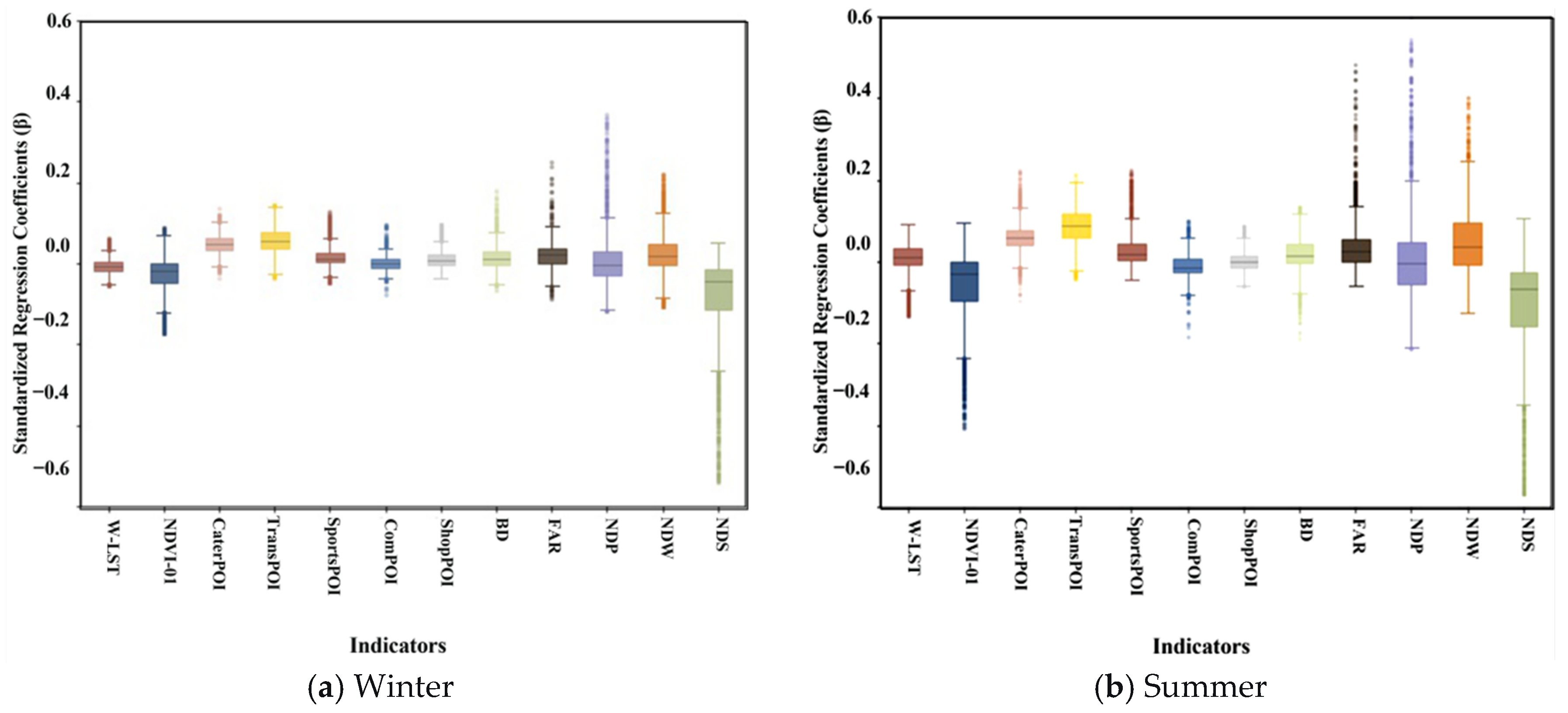
Figure 3a,b display boxplots of z-score standardized GWR coefficients (β) for winter and summer SVI, respectively. The distribution of β values not only reflects the mechanism of each influencing factor on the steady-state vitality of Wuhan City, but also reveals the differences in the influence mechanism of a certain factor on SVI in winter and summer. Specifically, six indicators—TransPOI, CaterPOI, NDW, SportsPOI, FAR, and BD—exhibit significant positive associations with SVI in both seasons, indicating that increases in these indicators generally enhance SVI in specific urban areas, further confirming that the provision of functional facilities and high development intensity support steady-state vitality. Among them, TransPOI has the most prominent impact on SVI, with a mean regression coefficient ( β ¯ ) of 0.206 in summer and 0.135 in winter; followed by CaterPOI, with β ¯ of 0.135 in summer and 0.116 in winter, indicating that the promoting effect of public transport accessibility and spatial clustering of dining facilities on SVI growth is approximately 16.4% stronger in summer than in winter; Regarding natural factors, LST shows a β ¯ of 0.073 for SVI in summer, compared with −0.040 in winter; the summer β ¯ is 82.5% higher than in winter. Vegetation-rich areas exhibit stronger positive associations with SVI in summer, consistent with NDVI showing 68.75% greater negative impact in summer ( β ¯ = −0.054) compared to winter ( β ¯ = −0.032), further proving the significant seasonal differentiation in the impact of natural elements on SVI.
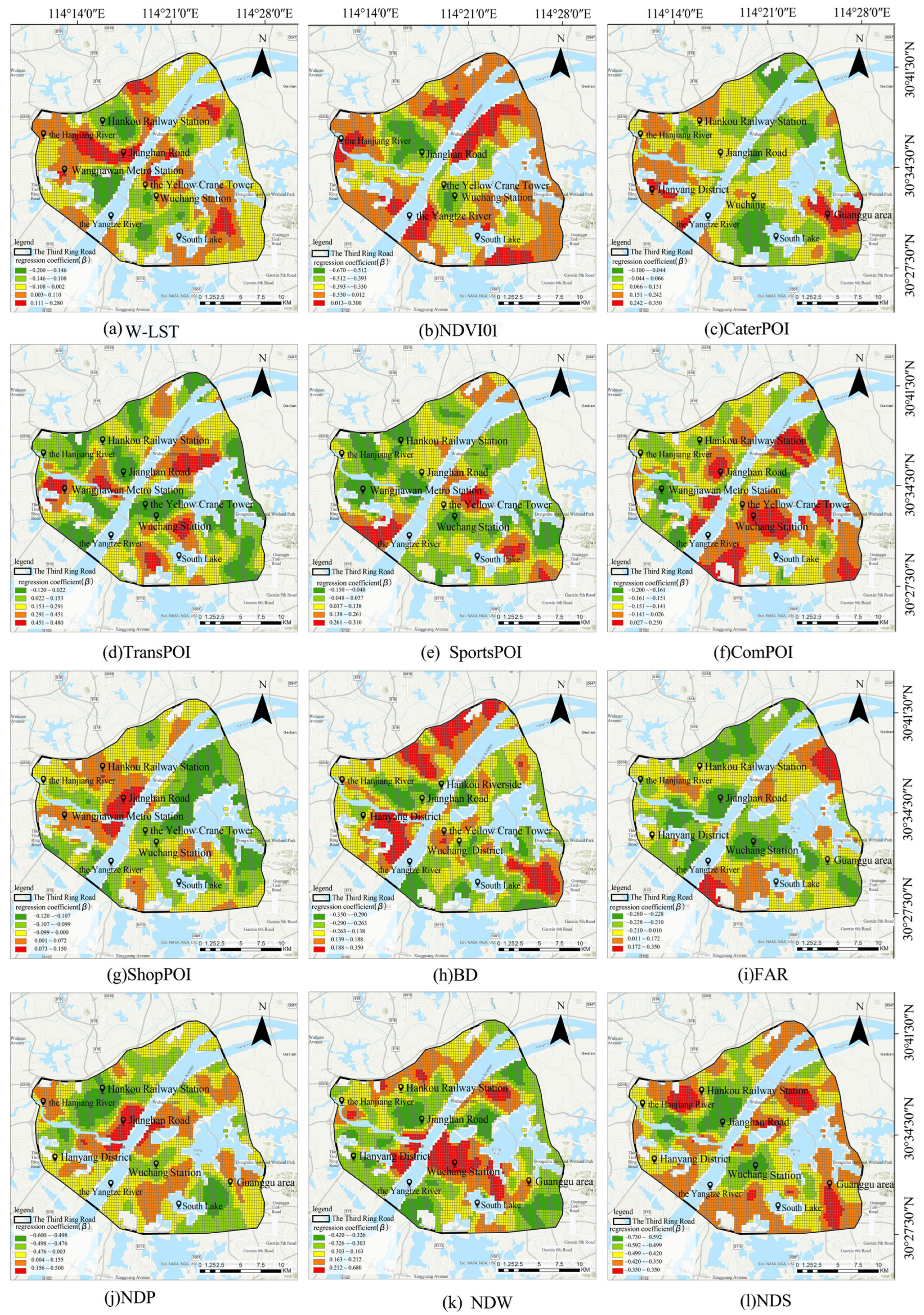
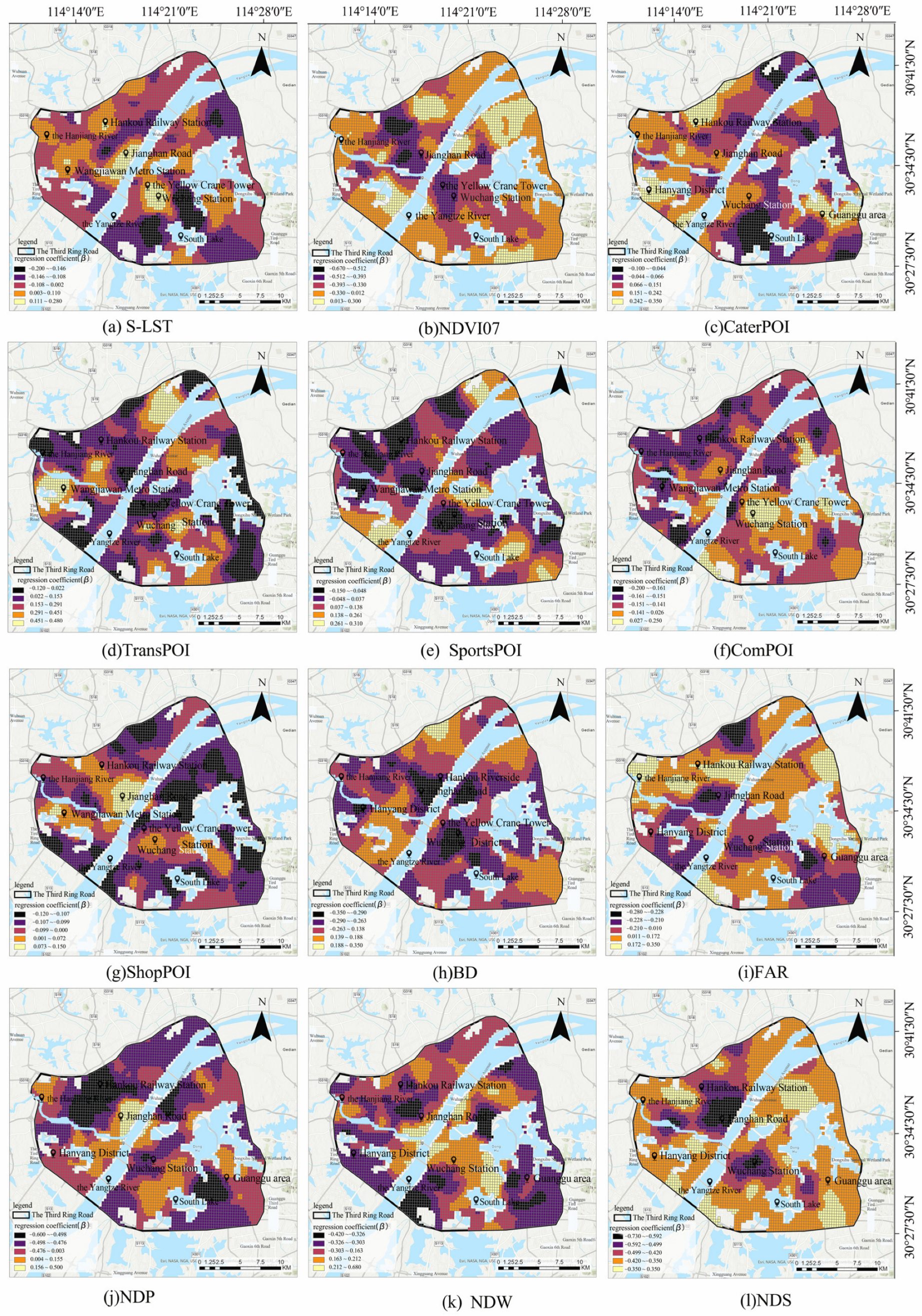
Further analysis of the factors influencing the spatial distribution of SVI. Figure 4 and Figure 5 display z-score standardized GWR coefficients (β) for winter and summer, respectively. First, regarding the influence of the natural environment, LST shows obvious seasonal and spatial differentiation in its effect on SVI. Comparing Figure 4a and Figure 5a, in winter, 70% of the study area shows positive β values for the effect of LST on SVI, with regions having surface temperatures of 11–13 °C exhibiting mean β values ranging from 0.053 to 0.140, indicating a significant promoting effect on SVI growth. In summer, areas with positive β values for LST effects on SVI account for 35% of the study area, with regions having surface temperatures of 40–43 °C showing β values concentrated further in the range of 0.111–0.280. Areas such as Jianghan Road, Wuchang Station, and the Yellow Crane Tower scenic area show higher population aggregation despite high summer temperatures, possibly because the attractiveness of these areas to public activities outweighs the negative effects of high summer temperatures on urban vitality. Figure 4b and Figure 5b indicate that NDVI effects on SVI are spatially consistent across seasons, with over 50% of areas along the Yangtze River showing that higher vegetation coverage corresponds to greater SVI growth. Specifically, in winter, SVI reaches its maximum when NDVI is 0.15–0.20, whereas in summer, the public prefers green spaces with NDVI ranging from 0.323 to 0.411.
Second, regarding travel purposes, the promoting effects of different types of POI on steady-state vitality exhibit significant spatiotemporal heterogeneity. As shown in Figure 4c–g and Figure 5c–g, among all POI types, CaterPOI (winter: β ¯ = 0.116, summer: β ¯ = 0.135) and TransPOI (winter: β ¯ = 0.135, summer: β ¯ = 0.206) have the best effect on the improvement of SVI. Specifically, Figure 4c shows that about 80% of the scope where CaterPOI promotes SVI growth are concentrated in Hanyang District and the Guanggu area. Figure 4f and Figure 5f both indicate that the area where ComPOI can significantly enhance SVI accounts for approximately 80% of the entire region, and it is mainly concentrated near the concentrated area of universities in Wuchang. Figure 5g shows that roughly 85% of the areas where ShopPOI has a strong citizen-attracting effect are distributed along the northern bank of the Yangtze River in summer. These observations further illustrate that the urban functional areas, such as densely populated universities and highly attractive commercial districts, can regulate and enhance the steady-state vitality.
Finally, the influence of built environmental on SVI exhibits little variation between summer and winter. Figure 4h–l and Figure 5h–l demonstrate that both BD and FAR have significant growth-promoting effects on SVI in more than 60% of the study areas. Meanwhile, NDP and NDW show positive effects on SVI growth in approximately 35% of the study area, mainly including the areas surrounding Hankou Riverside. Specifically, in these areas within roughly 800 m of water bodies, the regression coefficient (β) for SVI ranges mostly between 0.15 and 0.32 in both summer and winter, indicating that waterside spaces can largely drive the growth of SVI. On the other hand, NDS exhibits strong negative effects in central areas such as Jianghan Road and the Wuchang higher education zone, with β mostly ranging from −0.7 to −0.5, indicating that public transport accessibility plays a significant role in promoting SVI growth.

3.2. Analysis of Urban Dynamic Vitality

3.2.1. Spatiotemporal Distribution Characteristics of DVSD

Figure 6a–f and Figure 7a–f present dynamic urban vitality (DVSD) patterns through kernel density estimation (KDE), highlighting spatiotemporal contrasts between rest days and weekdays. Quantitative comparisons reveal the commonalities and differences in DVSD across rest days and weekdays. Regarding commonalities, areas with DVSD at level 5—representing the highest degree of population aggregation—account for 12.3% on rest days and 9.8% on weekdays, with 52.7% concentrated along the Hankou and Wuchang riverfronts, confirming the persistent attractiveness of these areas to citizens. Regarding differences, comparing Figure 6a–c and Figure 7a–c, on rest days, the area of the DVSD level-5 high-vitality cores at 12:00 nearly doubled compared with that at 9:00, while on weekdays, it decreased to about 85% of its 9:00 extent. In addition, at 12:00 on rest days, new level-5 DVSD areas also emerge in secondary centers such as the Wuchang Jiedaokou commercial district, and the Nanhu commercial district. This phenomenon is closely related to the midday shift in urban citizens’ activity from morning commuting to diverse activities such as shopping and dining, enabling vitality diffusion from the high-vitality core area to the sub-center. Notably, compared to weekdays, the formation and spread of DVSD peaks on rest days are delayed by approximately three hours, reflecting the critical influence of residents’ daily routines on population aggregation and activity. From 18:00 to 21:00, nighttime economic activities further increase the area of level-5 DVSD zones by 21%, indicating that the nighttime economy has a significant driving effect on population aggregation.

3.2.2. Analysis of VFI Cluster Result

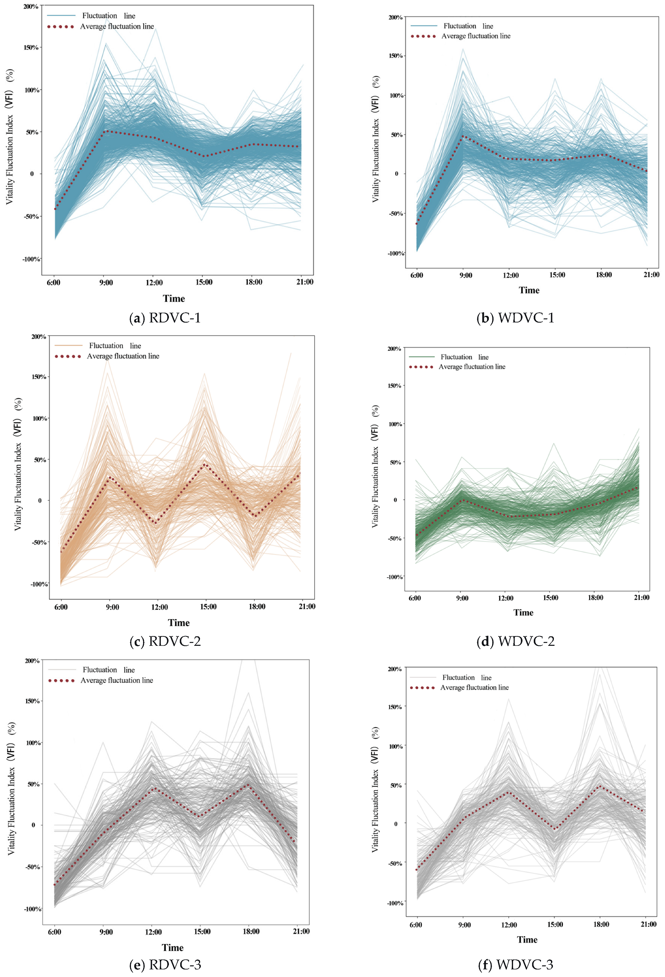
Figure 8 show the temporal variation in VFI for the six DVCs (RDVC-1, RDVC-2, RDVC-3, and WDVC-1, WDVC-2, WDVC-3), reflecting the increase or decrease in VFI in each grid unit relative to the daily average, clearly illustrating the rhythmic differences in vitality changes across grid units over time. By interpreting the six DVC time series line graphs in Figure 8a–f the temporal characteristics of the six DVCs were classified into state change patterns shown in Table 4.
As shown in Figure 8a,b, for both RDVC-1 and WDVC-1, VFI across all grids remains high from 9:00 to 21:00, indicating sustained high-intensity population aggregation, with crowds consistently in a high-high aggregation state. Specifically, the period from 6:00 to 9:00 on rest days and weekdays, represents the peak of citizens’ activity growth, with mean VFI values reaching around 52%, while during other periods VFI values remain at approximately 32%, reflecting stable high population aggregation. The distribution of these two DVC types is mainly concentrated in the central Jianghan District, Wuchang District, and certain large residential, educational, and commercial complexes within the study area, such as Shahu Park, Panahai International Plaza, Wuhan University, and Wuhan University of Technology—areas characterized by high population density. This high-intensity and long-duration vitality state is primarily the result of the combined influence of residential, service, and educational demands.
As shown in Figure 8c, grids corresponding to RDVC-2 exhibit an average VFI amplitude greater than 1.5σ, indicating that human activities display a pronounced periodic low-value fluctuation pattern. Specifically, in the corresponding study area, a large concentration of citizens occurs around 9:00, when the average VFI reaches approximately 27%. By 12:00, citizens’ activities begin to disperse outward, and the average VFI decreases to about –5%. After 15:00, the mean VFI rises again to about 50%, and from 18:00 to 21:00, evening activities drive a resurgence in population, exhibiting a “gather–disperse–regather” temporal fluctuation pattern. This pattern is primarily concentrated in residential and commercial areas along the Han River. The residential areas and universities in this region provide basic activity venues for people, and heightened weekend travel willingness generates periodic outbound demand.
Figure 8d shows that the standard deviation of mean VFI in the grids of the WDVC-2 study area is <0.3, indicating that crowd activity exhibits a stable low-low aggregation state. Specifically, in this area, the mean VFI fluctuates within ±20% from 9:00 to 21:00, with diurnal differences not exceeding 15%, and no pronounced aggregation or dispersion peaks, indicating that the activity rhythm in this area during weekdays is relatively stable. This DVC is mainly distributed in high-rise residential areas along the Yangtze River, with functional zones dominated by residential and educational land, accounting for approximately 55.8% of the total area, while commercial service land covers only 8.3%. This indicates that citizens’ activity is characterized by short-distance, low-mobility movements.
As shown in Figure 8e,f, the mean VFI values in areas corresponding to RDVC-3 and WDVC-3 exhibit a distinct bimodal fluctuation pattern, characterized by a low–medium–low variation in aggregation intensity. Specifically, from 9:00 to 12:00, the mean VFI reaches an initial peak, with an average value of approximately 50%, reflecting the morning concentration of citizens. After 12:00, citizens’ activities begin to disperse, leading to a decline in VFI values. A second aggregation peak occurs after 18:00, when the VFI again rises to around 50%. The areas influenced by the WDVC-3 are mainly distributed in large, well-connected commercial centers such as Wuhan Mall City and Yuehui Plaza, as well as educational zones such as Hubei University. This suggests that the midday and evening clustering of citizens is primarily driven by commuting and commercial activities. The areas influenced by the RDVC-3 are mainly located around the confluence of the Han River and the Yangtze River, as well as leisure and commercial zones such as Jianghan Road. In these areas, the first peak of population aggregation occurs around 12:00 noon in the waterfront recreational spaces, where the mean VFI reaches approximately 50%. After 18:00, the aggregation shifts toward nearby commercial nodes, forming a second peak, with the VFI average once again rising to about 50%.
Overall, the above analysis indicates that the fluctuation patterns of the intensity and vitality changes in the six types of DVCS with dynamic vitality in Wuhan City present four characteristics: continuous high-high aggregation (RDVC-1/WDVC-1); periodic low-value fluctuations (RDVC-2); continuous low-low aggregation (WDVC-2); and low-high-low aggregation (RDVC-3/WDVC-3).

3.2.3. Analysis of Influencing Indicators for Urban DVC Formation

This section will further examine from the perspective of dynamic vitality the influence mechanism of 14 factors in three types of evaluation indicators, namely travel purpose, natural environment and built environment, on the formation of different types of DVCS. Given the temporal coverage of Tencent location data, W-LST and NDVI-01 are selected as natural environment indicators. The corrected Akaike Information Criterion (AICc) values for the Global Logistic Regression (GLR) [49] and Geographically Weighted Logistic Regression (GWLR) models across various DVCs are as follows: WDVC-1 (7076.177, 6930.407), WDVC-2 (4532.110, 4342.707), WDVC-3 (5267.664, 5111.231), RDVC-1 (4674.239, 4534.116), RDVC-2 (2798.327, 2752.924), and RDVC-3 (3064.459, 2964.660). These results confirm that All GWLR models exhibit lower AICc values compared to GLR’s and it effectively captures the spatial relationships between the independent variables and DVCs. After GWLR analysis, Figure 8a–f present boxplots of z-score standardized GWLR coefficients (β), measuring the effect of each indicator on each DVC.
Analysis of Influencing Factors for RDVC-1 and WDVC-1
As shown in Figure 9a,b, the influencing factors of the two consistently high-high aggregation DVCs (RDVC-1, WDVC-1) exhibit significant differences. In the RDVC-1 pattern areas on rest days, NDS, NDP, FAR, and NDW have mean regression coefficients ( β ¯ ) of 0.101, 0.063, 0.083, and 0.055, respectively. All are positive, indicating significant positive effects on the formation of this pattern. These results indicate that areas farther from subway stations, parks, and water bodies, with higher development intensity, strongly attract people on rest day, maintaining high population aggregation. Meanwhile, NDVI01, W-LST, and TransPOI have mean regression coefficient ( β ¯ ) of −0.224, −0.3, and −0.151, respectively, exerting a significant negative effect on the formation of this pattern. This further indicates that areas with poorer vegetation cover, lower winter temperatures, and dense transportation facilities are less conducive to the formation of this pattern.
On weekdays, in WDVC-1 pattern areas, FAR, TransPOI, and ComPOI have β ¯ of 0.095, 0.068, and 0.061, respectively. All are positive, exerting significant positive effects on the formation of this pattern. These findings suggest that highly developed areas, transportation hubs, and office districts are the key factors of rapid population aggregation during the weekday morning peak (6:00–9:00). Conversely, NDS, CaterPOI, and SportsPOI have β ¯ of −0.204, −0.125, and −0.096, respectively, exerting significant negative effects on the formation of this pattern. To further explain the “commuter dominance” attribute of WDVC-1, its core demand is the aggregation of office workers during the morning rush hour. Areas too close to the subway will also be dispersed and weaken the aggregation effect of the crowd due to commuting. And leisure facilities such as restaurants and sports will also reduce the concentration of office functions.
Analysis of Influencing Factors of RDVC-2
As shown in Figure 10a, in RDVC-2 pattern areas, the mean regression coefficients ( β ¯ ) of NDS, NDW, NDP, SportsPOI, W-LST, and FAR are 0.178, 0.117, 0.067, 0.149, 0.043, and 0.041, respectively. All are positive, indicating significant positive effects on the formation of this pattern. These results indicate that far from subway stations, water bodies, and parks, coupled with well-developed sports facilities, suitable winter temperatures, and moderately high floor area ratio development, jointly support the periodic fluctuations of population aggregation in this area over time. The mean regression coefficients ( β ¯ ) of NDVI01, ComPOI, TransPOI, ShopPOI, and CaterPOI are −0.470, −0.329, −0.159, −0.078, and −0.044, respectively, all exerting significant negative effects on the formation of this pattern. The results indicate that a relatively high vegetation coverage rate and the concentration of office areas and shopping or leisure facilities, is actually not conducive to the formation of agglomeration patterns with periodic fluctuations in human activities. This could be attributed to the fact that the aforementioned factors result in a relatively stable state of agglomeration and dispersion of residents’ activities in the region, leading to low volatility in such activities.
Analysis of Influencing Factors of WDVC-2
As shown in Figure 10b, in WDVC-2 areas, the mean regression coefficients ( β ¯ ) of NDVI01, BD, SportsPOI, TransPOI, NDW, and FAR are 0.294, 0.263, 0.214, 0.186, and 0.125, respectively. All are positive, indicating significant positive effects on the formation of this pattern. These results indicate that high vegetation coverage, high building density, well-developed sports and transportation facilities, and proximity to water bodies are more conducive to periodic population fluctuations. However, the mean regression coefficients ( β ¯ ) of W-LST, ComPOI, ShopPOI, NDP, and CaterPOI are −0.110, −0.147, −0.145, −0.088, and −0.046, respectively, exerting significant negative effects on the formation of this pattern. he results also suggest that concentrations of company and commercial POI, lower winter temperatures, and greater distance to parks collectively inhibit the emergence of this dynamic vitality fluctuation pattern.
Analysis of Influencing Factors of RDVC-3 and WDVC-3
As shown in Figure 11a,b, the mean regression coefficients ( β ¯ ) of CaterPOI, NDVI01, ComPOI, and W-LST for RDVC-3 are 0.183, 0.138, 0.078, and 0.041, respectively, while for WDVC-3 they are 0.219, 0.277, 0.070, and 0.054. These factors exert significant positive effects on the formation of both RDVC-3 and WDVC-3 patterns. These results indicate that the distribution of catering facilities and winter vegetation coverage play key roles in guiding population aggregation and dispersion. Moreover, under the combined influence of commercial service facilities and environmental comfort, two distinct peaks of population aggregation emerge during midday and early evening. The mean regression coefficients ( β ¯ ) of NDW, NDS, and BD for RDVC-3 are −0.217, −0.192, and −0.075, respectively, whereas for WDVC-3 they are 0.002, 0.151, and 0.001. These factors reveal substantial differences in the mechanisms shaping RDVC-3 and WDVC-3. Specifically, population aggregation on rest days tends to concentrate in areas with well-developed commercial facilities and proximity to subway stations and water bodies, reflecting a leisure-oriented tendency, whereas on weekdays, the impact of commuting and rigid travel demands is dominant.

4. Discussion

4.1. Summary of Findings

We systematically analyzed the spatio-temporal characteristics and driving mechanisms of the vitality in the main urban area of Wuhan based on the temporal and spatial distribution patterns of steady-state vitality and dynamic vitality. Overall, from a steady-state perspective, the urban vitality of Wuhan presents a polycentric agglomeration pattern characterized by high vitality in the urban core and low vitality in the peripheral areas, with distinct vitality corridors formed along major traffic arteries. In contrast, from a dynamic perspective, four main patterns of human agglomeration and dispersion have emerged on the basis of this stable vitality pattern. The key conclusions in both steady-state and dynamic aspects are systematically summarized and sorted out, providing scientific evidence for optimizing urban planning layout, transportation network system and public service resource allocation.

4.1.1. Mechanisms of Polycentric Steady-State Vitality

Based on the analysis results of steady-state vitality, we identify a distinct polycentric structure in Wuhan’s central districts, with 53% of Level-5 SVI high-vitality core zones concentrated in commercial districts, universities, and transportation hubs. This spatial structure further confirms that commercial districts and transportation hubs are the core driving forces of urban vitality [24]. Temporally, population aggregation is stronger in summer, with the area of Level-5 high-vitality core zones expanding nearly sixfold compared with winter. Further analysis reveals that the spatial distribution of SVI within the study area is jointly influenced by built environment, travel purpose, and natural factors. The results indicate that areas with high floor area ratios and dense buildings effectively enhance the regional attractiveness of commercial spaces [30].

4.1.2. Mechanisms of Dynamic Vitality DVC

During both rest days and weekends, over 50% of the high-vitality areas with a DVSD level of 5 are primarily concentrated along the riverside zones of Hankou and Wuchang. The DVSD level-5 areas account for 12.3% of the total study area on rest day and 9.8% on weekdays. These results indicate that waterfront zones and core commercial clusters exert strong attractiveness to urban citizens. However, at 9:00 on rest days, the area classified as DVSD level 5 decreases by 21% compared with the same period on weekdays, suggesting that the reduction in commuting activities on rest days leads to a delayed vitality peak.
The synergistic efficiency among urban functions, transportation, and the natural environment plays a critical role in shaping urban vitality [25]. Moreover, the vitality formation mechanisms of different DVCs are closely related to the functional utilization of urban spaces. During weekdays, the vitality areas represented by the WDVC-1 correspond primarily to office zones, where urban vitality is mainly driven by commuting behavior. TransPOI ( β ¯ = 0.068) and ComPOIs ( β ¯ = 0.061) exert significant positive effects on the formation of this dynamic vitality pattern. The vitality mechanism of WDVC-2, is mainly reflected in the emerging residential areas along the Yangtze River, where weekday residents’ activities are concentrated within a walkable living radius. This finding suggests that newly developed residential communities should incorporate metro stations and riverside greenways within a 15 min living circle to enhance accessibility and daily vitality [31,51]. WDVC-3 exhibits a bimodal vitality mechanism, with two peaks occurring around 12:00 (lunchtime) and 18:00 (after work), reflecting citizens’ dining, leisure, and commuting behaviors. On rest days, RDVC-1 features a sustained high level of population aggregation from 9:00 to 21:00, with the mean VFI exceeding about 25% and the maximum reaching 52%. The affected areas are primarily concentrated in commercial and educational zones. RDVC-2 demonstrates a cyclical fluctuation between population aggregation and dispersion, emphasizing the interaction between urban functions, transport accessibility, and environmental settings. RDVC-3 is mainly distributed around large commercial complexes, metro stations, and well-vegetated areas, where leisure-oriented urban spaces exhibit higher citizens’ concentration at midday and in the evening.

4.1.3. The Interactive Relationship Between Steady-State and Dynamic Vitality

The spatial overlap between SVI level-5 high-vitality core areas and WDVC-1 zones with a daily average VFI above 30% confirms that static vitality provides the foundation for dynamic vitality. Specifically, TransPOI ( β ¯ = 0.206) and CaterPOI ( β ¯ = 0.135) sustain high steady-state vitality by enhancing long-term functional attractiveness in summer. On this basis, the WDVC-1 further verifies that, under conditions of higher floor area ratio (FAR: β ¯ = 0.095) and transportation POI (TransPOI: β ¯ = 0.068), the degree of population aggregation increases significantly within certain short time intervals—such as a 50% surge in VFI during the morning peak—indicating a coexistence of long-term stability and short-term fluctuation in urban vitality. This integrative mechanism breaks through the conventional separation between steady-state and dynamic vitality analyses, providing a new perspective for urban planning. In high-vitality core areas, steady vitality should be maintained by strengthening the construction of commercial and transport facilities, while dynamic vitality can be enhanced through adaptive public service provisions—for instance, introducing mobile vendors during peak hours. Conversely, in peripheral zones with lower vitality, planners should leverage ecological advantages such as urban parks and natural landscapes to foster time-specific dynamic vitality growth points, and subsequently improve steady-state vitality through functional reinforcement.

4.2. Implication and Limitation

Nevertheless, several limitations should be acknowledged in this study. First, there is the issue of temporal misalignment among data from different sources. The mobile signaling data, Tencent application data, and built environment data adopted in this study are derived from different years. They do not reflect urban-related data at the same time point, which may lead to certain biases in the research results on urban vitality. Therefore, future research should strive to acquire multi-source data for a unified time period to construct an analytical framework with temporal consistency. Second, this study adopted the method of architectural theoretical analysis to examine the spatial overlap of steady-state vitality and dynamic vitality patterns. The quantitative research on the interrelationship between steady-state and dynamic vitality is insufficient, and it remains to be performed to construct a quantitative framework to explore the underlying correlations in depth.

5. Conclusions

Coordinating long-term urban planning with short-term management needs is essential for promoting sustainable urban development. This study integrates both steady-state and dynamic perspectives of urban vitality by utilizing mobile base-station signaling data and Tencent location-based big data. Through a combination of k-means clustering, GWR and GWLR, the study reveals the spatial–temporal characteristics and influencing factors of urban vitality across multiple scales. The findings provide a scientific basis for the refined optimization of urban planning and the allocation of public environmental resources. The main conclusions are as follows:
(a)
From the perspective of steady-state vitality, the central districts of Wuhan within the Third Ring Expressway demonstrate a polycentric structure, with commercial districts, universities, and transportation hubs forming the core zones of high vitality. Specifically, over 63% of the areas classified as level-5 high-vitality cores (SVI = 5) are occupied by university campuses and commercial centers, where factors such as TransPOI (β > 0.18) and CaterPOI (β > 0.11) exert significant positive effects on the formation of high vitality. Moreover, the area of level-5 SVI high-vitality zones in summer is approximately 5.97 times larger than in winter, indicating a pronounced seasonal variation in the effects of natural elements on steady-state vitality. This also verifies that large Chinese cities exhibit a polycentric vitality structure with mixed functions, providing specific practical directions for the optimal spatial functional layout of Wuhan’s urban space.
(b)
The spatiotemporal distribution of dynamic vitality exhibits distinct patterns between weekdays and rest day. Compared with rest days, weekday population aggregation peaks occur approximately three hours earlier—around 9:00—mainly driven by commuting demand. In contrast, on rest days, the peak area of level-5 DVSD zones appears around 12:00 and is primarily influenced by nearby leisure facilities and green spaces. Moreover, due to residents’ recreational activities on rest days, the area of level-5 DVSD zones at 21:00 is 21% larger than that on weekdays. This study reveals distinct urban vitality patterns between weekdays and rest days. Accordingly, urban management should adopt time-differentiated strategies: prioritizing commuting efficiency on weekdays and focusing on the development of leisure and nighttime economies on rest days, so as to achieve the optimal allocation of spatial resources.
(c)
The spatial aggregation and dispersion characteristics of dynamic vitality are influenced by multiple factors. FAR (β > 0.083) serves as a key determinant of the RDVC-1 and WDVC-1 patterns, which represent areas of sustained high-density population aggregation and maintain average VFI values above 25% throughout the day. The RDVC-2 typically occurs in areas distant from metro stations (NDS: β ¯ = 0.178), with low vegetation coverage (NDVI01: β ¯ = −0.470) and a sparse distribution of commercial facilities (ComPOI: β ¯ = −0.329), exhibiting pronounced periodic fluctuations. In contrast, green coverage (NDVI01: β ¯ = 0.294) and building density (BD: β ¯ = 0.263) exert strong positive effects on the formation of the WDVC-2 pattern, characterized by low—low aggregation of citizens’ activities. This pattern is primarily distributed in residential and educational—research land, accounting for approximately 55.8% of such areas. Both RDVC-3 and WDVC-3 patterns display bimodal fluctuations in VFI values, with variations primarily driven by CaterPOI (β > 0.18) and NDVI01 (β > 0.13). By systematically deconstructing the multi-pattern differentiation mechanism of urban dynamic vitality, this study proposes a pattern-oriented urban governance approach, whose core lies in the implementation of precise and differentiated planning and management based on distinct spatial agglomeration and dispersion characteristics.
(d)
The areas characterized by high levels of both steady-state and dynamic vitality exhibit a substantial degree of spatial overlap, primarily concentrated around commercial districts and transportation hubs. In terms of steady-state vitality, over 90% of level-5 SVI high-vitality zones coincide with regions of equivalent vitality under dynamic conditions. Furthermore, these zones overlap by approximately 68% with zones of continuous high population aggregation, where the average VFI exceeds 30% (corresponding to RDVC-1 and WDVC-1 patterns).

Author Contributions

Conceptualization, X.T. and K.L.; methodology, K.L.; software, X.T. and D.X.; formal analysis, X.T.; investigation, Y.F.; resources, K.L.; data curation, Y.F. and D.X.; writing—original draft preparation, K.L., X.T., Y.F. and D.X.; writing—review and editing, X.T. and K.L.; visualization, X.T.; supervision, K.L.; project administration, K.L.; funding acquisition, K.L. All authors have read and agreed to the published version of the manuscript.

Funding

This research was funded by the Basic Work of Science and Technology of China (Grant No. 2013FY112500) and the National Natural Science Foundation of China (Grant No. 51208389).

Data Availability Statement

Data available on request due to restrictions legal.

Acknowledgments

During the preparation of this study, the author(s) used [ChatGPT, 4.0] for the purposes of [polish the language and improve readability]. The authors have reviewed and edited the output and take full responsibility for the content of this publication. We would like to express our sincere gratitude to José Ramón Albiol Ibáñez from Universitat Politècnica de València for his participation in several discussions during the research process of this paper.

Conflicts of Interest

The authors declare no conflicts of interest. The funder had no role in the design of the study; in the collection, analyses, or interpretation of data; in the writing of the manuscript; or in the decision to publish the results.

Abbreviations

The following abbreviations are used in this manuscript:
GWRGeographically Weighted Regression
GWLRGeographically Weighted Logistic Regression
GLRGlobal Logistic Regression
POIPoints of interest
SDGsSustainable Development Goals
OLSOrdinary Least Squares
W-LSTWinter Land Surface Temperature
S-LSTSummer Land Surface Temperature
NDVINormalized Difference Vegetation Index
CaterPOICatering points of interest
TransPOITransportation points of interest
ComPOICompany points of interest
ShopPOIShopping points of interest
BDBuilding Density
FARFloor Area Ratio
NDPDistance to Park
NDWDistance to Waterbody
NDSDistance to Subway
SVI Steady-state Vitality Index
DVSD Dynamic Vitality Spatial Density
VFIVitality Fluctuation Index
DVC Dynamic Vitality Cluster
WDVC Weekday Dynamic Vitality Cluster
RDVC Rest-day Dynamic Vitality Cluster

References

  1. Jiang, Y.; Huang, Z.; Zhou, X.; Chen, X. Evaluating the Impact of Urban Morphology on Urban Vitality: An Exploratory Study Using Big Geo-Data. Int. J. Digit. Earth 2024, 17, 2327571. [Google Scholar] [CrossRef]
  2. Liu, S.; Zhang, L.; Long, Y. Urban Vitality Area Identification and Pattern Analysis from the Perspective of Time and Space Fusion. Sustainability 2019, 11, 4032. [Google Scholar] [CrossRef]
  3. Jiang, Y.; Chen, Z.; Sun, P. Urban Shrinkage and Urban Vitality Correlation Research in the Three Northeastern Provinces of China. Int. J. Environ. Res. Public Health 2022, 19, 10650. [Google Scholar] [CrossRef]
  4. Zhang, P.; Zhang, T.; Fukuda, H.; Ma, M.H. Evidence of Multi-Source Data Fusion on the Relationship between the Specific Urban Built Environment and Urban Vitality in Shenzhen. Sustainability 2023, 15, 6869. [Google Scholar] [CrossRef]
  5. Jacobs, J. The Death and Life of Great American Cities; Random House: New York, NY, USA, 1961. [Google Scholar]
  6. Li, Q.; Cui, C.; Liu, F.; Wu, Q.; Run, Y.; Han, Z. Multidimensional Urban Vitality on Streets: Spatial Patterns and Influence Factor Identification Using Multi-Source Urban Data. ISPRS Int. J. Geo-Inf. 2021, 11, 2. [Google Scholar] [CrossRef]
  7. Yue, W.; Chen, Y.; Zhang, Q.; Liu, Y. Spatial Explicit Assessment of Urban Vitality Using Multi-Source Data: A Case of Shanghai, China. Sustainability 2019, 11, 638. [Google Scholar] [CrossRef]
  8. Kang, C.-D. Measuring Urban Form and Its Effects on Urban Vitality in Seoul, South Korea: Urban Morphometric Approach. J. Urban Plan. Dev. 2024, 150, 05024019. [Google Scholar] [CrossRef]
  9. Paköz, M.Z.; Işık, M. Rethinking urban density, vitality and healthy environment in the post-pandemic city: The case of istanbul. Cities 2022, 124, 103598. [Google Scholar] [CrossRef] [PubMed]
  10. Wu, W.; Niu, X. Influence of Built Environment on Urban Vitality: Case Study of Shanghai Using Mobile Phone Location Data. J. Urban Plan. Dev. 2019, 145, 04019035. [Google Scholar] [CrossRef]
  11. Kim, Y.-L. Data-Driven Approach to Characterize Urban Vitality: How Spatiotemporal Context Dynamically Defines Seoul’s Nighttime. Int. J. Geogr. Inf. Sci. 2020, 34, 1235–1256. [Google Scholar] [CrossRef]
  12. Kim, Y.-L. Seoul’s wi-fi hotspots: Wi-fi access points as an indicator of urban vitality. Comput. Environ. Urban Syst. 2018, 72, 13–24. [Google Scholar] [CrossRef]
  13. Delclòs-Alió, X.; Gutiérrez, A.; Miralles-Guasch, C. The Urban Vitality Conditions of Jane Jacobs in Barcelona: Residential and Smartphone-Based Tracking Measurements of the Built Environment in a Mediterranean Metropolis. Cities 2019, 86, 220–228. [Google Scholar] [CrossRef]
  14. Sun, Y.; Wen, Z.; Tian, D.; Zhang, M.; Hou, Y. Study on Community Detection Method for Morning and Evening Peak Shared Bicycle Trips in Urban Areas: A Case Study of Six Districts in Beijing. Buildings 2023, 13, 2446. [Google Scholar] [CrossRef]
  15. Batty, M. Cities and Complexity: Understanding Cities with Cellular Automata, Agent-Based Models, and Fractals; The MIT Press: Cambridge, MA, USA, 2007. [Google Scholar]
  16. Whiteley, T.D.; Avitabile, D.; Siebers, P.-O.; Robinson, D.; Owen, M.R. Modelling the emergence of cities and urban patterning using coupled integro-differential equations. J. R. Soc. Interface 2022, 19, 20220176. [Google Scholar] [CrossRef]
  17. Cao, Y.; He, X.; Zhou, C.; Cao, Y.; He, X.; Zhou, C. Characteristics and influencing factors of population migration under different population agglomeration patterns—A case study of urban agglomeration in China. Sustainability 2023, 15, 6909. [Google Scholar] [CrossRef]
  18. Ding, L.; Song, X.; Niu, X. Characters of functional linkage of urban spatial structure: A case study of shanghai central city. City Plan. Rev. 2019, 43, 107–116. [Google Scholar]
  19. Gómez-Varo, I.; Delclòs-Alió, X.; Miralles-Guasch, C. Jane Jacobs Reloaded: A Contemporary Operationalization of Urban Vitality in a District in Barcelona. Cities 2022, 123, 103565. [Google Scholar] [CrossRef]
  20. Doan, Q.C.; Ma, J.; Chen, S.; Zhang, X. Nonlinear and Threshold Effects of the Built Environment, Road Vehicles and Air Pollution on Urban Vitality. Landsc. Urban Plan. 2025, 253, 105204. [Google Scholar] [CrossRef]
  21. Elliott, H.; Eon, C.; Breadsell, J. Improving City Vitality through Urban Heat Reduction with Green Infrastructure and Design Solutions: A Systematic Literature Review. Buildings 2020, 10, 219. [Google Scholar] [CrossRef]
  22. Zumelzu, A.; Barrientos-Trinanes, M. Analysis of the effects of urban form on neighborhood vitality: Five cases in Valdivia, Southern Chile. J. Hous. Built Environ. 2019, 34, 897–925. [Google Scholar] [CrossRef]
  23. Pan, C.; Zhou, J.; Huang, X. Impact of Check-In Data on Urban Vitality in the Macao Peninsula. Sci. Program. 2021, 2021, 7179965. [Google Scholar] [CrossRef]
  24. Huang, Y.; Du, J.; Chen, M.; Lin, Y.; Huang, S.; Cai, Y. Evaluating the spatial-temporal impact of urban nature on urban vitality in vancouver: A social media and GPS data approach. Land Use Policy 2026, 160, 107824. [Google Scholar] [CrossRef]
  25. Sung, H.; Lee, S. Residential Built Environment and Walking Activity: Empirical Evidence of Jane Jacobs’ Urban Vitality. Transp. Res. Part D 2015, 41, 318–329. [Google Scholar] [CrossRef]
  26. Liu, D.X.; Shi, Y.S. The Influence Mechanism of Urban Spatial Structure on Urban Vitality Based on Geographic Big Data: A Case Study in Downtown Shanghai. Buildings 2022, 12, 569. [Google Scholar] [CrossRef]
  27. Paköz, M.Z.; Yaratgan, D.; Şahin, A. Re-mapping urban vitality through jane jacobs’ criteria: The case of kayseri, turkey. Land Use Policy 2022, 114, 105985. [Google Scholar] [CrossRef]
  28. Fu, R.; Zhang, X.; Yang, D.; Cai, T.; Zhang, Y. The Relationship between Urban Vibrancy and Built Environment: An Empirical Study from an Emerging City in an Arid Region. Int. J. Environ. Res. Public Health 2021, 18, 525. [Google Scholar] [CrossRef] [PubMed]
  29. Mouratidis, K.; Poortinga, W. Built Environment, Urban Vitality and Social Cohesion: Do Vibrant Neighborhoods Foster Strong Communities? Landsc. Urban Plan. 2020, 204, 103951. [Google Scholar] [CrossRef]
  30. Zeng, C.; Song, Y.; He, Q.; Shen, F. Spatially Explicit Assessment on Urban Vitality: Case Studies in Chicago and Wuhan. Sustain. Cities Soc. 2018, 40, 296–306. [Google Scholar] [CrossRef]
  31. Zhang, Z.; Zhang, Y.; He, T.; Xiao, R. Urban Vitality and Its Influencing Factors: Comparative Analysis Based on Taxi Trajectory Data. IEEE J. Sel. Top. Appl. Earth Obs. Remote Sens. 2022, 15, 5102–5114. [Google Scholar] [CrossRef]
  32. Chen, M.; Cai, Y.; Guo, S.; Sun, R.; Song, Y.; Shen, X. Evaluating implied urban nature vitality in san francisco: An interdisciplinary approach combining census data, street view images, and social media analysis. Urban For. Urban Green. 2024, 95, 128289. [Google Scholar] [CrossRef]
  33. Lopes, M.N.; Camanho, A.S. Public green space use and consequences on urban vitality: An assessment of European cities. Soc. Indic. Res. 2013, 113, 751–767. [Google Scholar] [CrossRef]
  34. Peng, X.; Jin, Y.; Girling, C.; Wu, S. Indicators Shaping Urban Greenspace Spatial Performance in China: A Systematic Review of the Literature. World Dev. 2025, 195, 107148. [Google Scholar] [CrossRef]
  35. Wang, L.; Li, R.; Jia, J.; Zhai, Y.; Tian, Y.; Xu, D.; Chen, Y.; Zhang, X.; Ren, Z.; Ye, Z.; et al. Integrating Morphology and Vitality to Quantify Seasonal Contributions of Urban Functional Zones to Thermal Environment. Sustain. Cities Soc. 2025, 120, 106136. [Google Scholar] [CrossRef]
  36. Griffin, M.; Nordstrom, B.W.; Scholes, J.; Joncas, K.; Gordon, P.; Krivenko, E.; Haynes, W.; Higdon, R.; Stewart, E.; Kolker, N.; et al. A Case Study: Analyzing City Vitality with Four Pillars of Activity—Live, Work, Shop, and Play. Big Data 2016, 4, 60–66. [Google Scholar] [CrossRef] [PubMed]
  37. Ahas, R.; Aasa, A.; Yuan, Y.; Raubal, M.; Smoreda, Z.; Liu, Y.; Ziemlicki, C.; Tiru, M.; Zook, M. Everyday space–time geographies: Using mobile phone-based sensor data to monitor urban activity in harbin, paris, and tallinn. Int. J. Geogr. Inf. Sci. 2015, 29, 2017–2039. [Google Scholar] [CrossRef]
  38. Liu, S.; Zhang, L.; Long, Y.; Long, Y.; Xu, M. A New Urban Vitality Analysis and Evaluation Framework Based on Human Activity Modeling Using Multi-Source Big Data. ISPRS Int. J. Geo-Inf. 2020, 9, 617. [Google Scholar] [CrossRef]
  39. Annunziata, A.; Garau, C. A Literature Review on the Assessment of Vitality and Its Theoretical Framework. Emerging Perspectives for Geodesign in the Urban Context. In Computational Science and Its Applications—ICCSA 2021; Gervasi, O., Murgante, B., Misra, S., Garau, C., Blečić, I., Taniar, D., Apduhan, B.O., Rocha, A.M.A.C., Tarantino, E., Torre, C.M., Eds.; Springer: Cham, Switzerland, 2021; Volume 12958, pp. 305–322. [Google Scholar] [CrossRef]
  40. Gan, X.Y.; Huang, L.; Wang, H.Y.; Mou, Y.C.; Wang, D.; Hu, A. Optimal Block Size for Improving Urban Vitality: An Exploratory Analysis with Multiple Vitality Indicators. J. Urban Plan. Dev. 2021, 147, 04021027. [Google Scholar] [CrossRef]
  41. Cai, J.; Yu, H.; Chen, M.; Pan, H. Using Multi-Source Geospatial Big Data to Identify the Structure of Polycentric Cities. Remote Sens. Environ. 2017, 202, 210–221. [Google Scholar] [CrossRef]
  42. Liu, H.; Gou, P.; Xiong, J. Vital Triangle: A New Concept to Evaluate Urban Vitality. Comput. Environ. Urban Syst. 2022, 98, 101886. [Google Scholar] [CrossRef]
  43. Wu, W.; Xu, L.; Zhao, K. Spatial Nonlinear Effects of Urban Vitality under the Constraints of Development Intensity and Functional Diversity. Alex. Eng. J. 2023, 77, 645–656. [Google Scholar] [CrossRef]
  44. Mahato, R.K.; Htike, K.M.; Sornlorm, K.; Koro, A.B.; Kafle, A.; Sharma, V. A Spatial Autocorrelation Analysis of Road Traffic Accidents by Severity Using Moran’s I Spatial Statistics: A Study from Nepal 2019–2022. BMC Public Health 2024, 24, 3086. [Google Scholar] [CrossRef]
  45. Xie, Y.; Shang, C.; Deng, X. Evolution of Urban Vitality Drivers from 2014 to 2022: A Case Study of Kunming, China. Int. J. Environ. Sci. Technol. 2025, 22, 11459–11472. [Google Scholar] [CrossRef]
  46. Shi, J.G.; Miao, W. Urban Vitality Evaluation and Spatial Correlation Research: A Case Study from Shanghai, China. Land 2021, 10, 1195. [Google Scholar] [CrossRef]
  47. Lykostratis, K.; Giannopoulou, M.; Roukouni, A. Measuring Urban Configuration: A GWR Approach. In New Metropolitan Perspectives; Calabrò, F., Della Spina, L., Bevilacqua, C., Eds.; Springer: Cham, Switzerland, 2019; Volume 100, pp. 479–488. [Google Scholar] [CrossRef]
  48. Sulekan, A.; Jamaludin, S.S.S. Review on Geographically Weighted Regression (GWR) Approach in Spatial Analysis. Malays. J. Fundam. Appl. Sci. 2020, 16, 173–177. [Google Scholar] [CrossRef]
  49. Qu, X.; Xiao, X.; Zhu, X.; Shao, Z.; Wang, M.; Wu, H.; Zhao, H.; Gong, J.; Li, D. ST-GWLR: Combining Geographically Weighted Logistic Regression and Spatiotemporal Hotspot Trend Analysis to Explore the Effect of Built Environment on Traffic Crash. Geo-Spat. Inf. Sci. 2024, 27, 1017–1034. [Google Scholar] [CrossRef]
  50. Basu, T.; Das, A.; Pereira, P. Exploring the Drivers of Urban Expansion in a Medium-Class Urban Agglomeration in India Using Remote Sensing Techniques and Geographically Weighted Models. Geogr. Sustain. 2023, 4, 150–160. [Google Scholar] [CrossRef]
  51. Qin, J.; Wang, Z.; Sheng, Y.; Xue, L.; Cai, X.; Zhang, K. Relationship between the Built Environment and Urban Vitality of Nanjing’s Central Urban Area Based on Multi-Source Data. Environ. Plan. B Urban Anal. City Sci. 2025, 52, 168–185. [Google Scholar] [CrossRef]
  52. Zafri, N.M.; Khan, A. Using Geographically Weighted Logistic Regression (GWLR) for Pedestrian Crash Severity Modeling: Exploring Spatially Varying Relationships with Natural and Built Environment Factors. IATSS Res. 2023, 47, 325–334. [Google Scholar] [CrossRef]
  53. Sun, H.; Chen, Y.; Lai, J.; Wang, Y.; Liu, X. Identifying Tourists and Locals by K-Means Clustering Method from Mobile Phone Signaling Data. J. Transp. Eng. Part A Syst. 2021, 147, 04021070. [Google Scholar] [CrossRef]
  54. Dong, Y.H.; Peng, F.L.; Guo, T.F. Quantitative Assessment Method on Urban Vitality of Metro-Led Underground Space Based on Multi-Source Data: A Case Study of Shanghai Inner Ring Area. Tunn. Undergr. Space Technol. 2021, 116, 104108. [Google Scholar] [CrossRef]
  55. Iamtrakul, P.; Chayphong, S.; Panuwatwanich, K. A Comprehensive Exploration of Urban Spatial Economic Vitality through the Application of the Node-Place Model. J. Urban Des. 2025, 1–15. [Google Scholar] [CrossRef]
  56. He, S.; Zhang, Z.; Yu, S.; Xia, C.; Tung, C.-L. Investigating the Effects of Urban Morphology on Vitality of Community Life Circles Using Machine Learning and Geospatial Approaches. Appl. Geogr. 2024, 167, 103287. [Google Scholar] [CrossRef]
  57. Yang, H.; Zheng, L.; Wang, Y.; Li, J.; Zhang, B.; Bi, Y. Quantifying the Relationship between Land Use Intensity and Ecosystem Services’ Value in the Hanjiang River Basin: A Case Study of the Hubei Section. Int. J. Environ. Res. Public Health 2022, 19, 10950. [Google Scholar] [CrossRef]
  58. Lai, Y.N.; Lv, Z.; Chen, C.M.; Liu, Q. Exploring Employment Spatial Structure Based on Mobile Phone Signaling Data: The Case of Shenzhen, China. Land 2022, 11, 983. [Google Scholar] [CrossRef]
  59. Wang, L.J.; Wu, X.; He, Y. Exploring the Urban Structure of Recreational Spaces through Residents’ Mobility Behavior Using Mobile Phone Signaling Data. J. Urban Plan. Dev. 2025, 151, 05025011. [Google Scholar] [CrossRef]
  60. Zheng, S.; Zheng, J. Assessing the Completeness and Positional Accuracy of OpenStreetMap in China. In Thematic Cartography for the Society; Bandrova, T., Konecny, M., Zlatanova, S., Eds.; Springer: Cham, Switzerland, 2014; pp. 171–189. [Google Scholar] [CrossRef]
  61. Shen, Z.; Shi, H.; Jiang, Y.; Sun, Z. Diurnal Variation in the Urban Thermal Environment and Its Relationship to Human Activities in China: A Tencent Location-Based Service Geographic Big Data Perspective. Environ. Sci. Pollut. Res. 2024, 31, 14218–14228. [Google Scholar] [CrossRef]
  62. Li, Z.; Wu, H.; Duan, S.; Zhao, W.; Ren, H.; Liu, X.; Leng, P.; Tang, R.; Ye, X.; Zhu, J.; et al. Satellite Remote Sensing of Global Land Surface Temperature: Definition, Methods, Products, and Applications. Rev. Geophys. 2023, 61, e2022RG000777. [Google Scholar] [CrossRef]
  63. Chen, Y.; Yang, J.; Yu, W.B.; Ren, J.Y.; Xiao, X.M.; Xia, J.C. Relationship between Urban Spatial Form and Seasonal Land Surface Temperature under Different Grid Scales. Sustain. Cities Soc. 2023, 89, 104374. [Google Scholar] [CrossRef]
  64. Kikon, N.; Kumar, D.; Ahmed, S.A. Quantitative Assessment of Land Surface erature and Vegetation Indices on a Kilometer Grid Scale. Environ. Sci. Pollut. Res. 2023, 30, 107236–107258. [Google Scholar] [CrossRef]
  65. Zhang, X.C.; Sun, Y.R.; Chan, T.O.; Huang, Y.; Zheng, A.Y.; Liu, Z. Exploring Impact of Surrounding Service Facilities on Urban Vibrancy Using Tencent Location-Aware Data: A Case of Guangzhou. Sustainability 2021, 13, 444. [Google Scholar] [CrossRef]
  66. Guo, X.; Chen, H.; Yang, X. An Evaluation of Street Dynamic Vitality and Its Influential Factors Based on Multi-Source Big Data. ISPRS Int. J. Geo-Inf. 2021, 10, 143. [Google Scholar] [CrossRef]
  67. Zhu, J.; Lu, H.; Zheng, T.; Rong, Y.; Wang, C.; Zhang, W.; Yan, Y.; Tang, L. Vitality of Urban Parks and Its Influencing Factors from the Perspective of Recreational Service Supply, Demand, and Spatial Links. Int. J. Environ. Res. Public Health 2020, 17, 1615. [Google Scholar] [CrossRef] [PubMed]
  68. Kumar, V.; Vuilliomenet, A. Urban Nature: Does Green Infrastructure Relate to the Cultural and Creative Vitality of European Cities? Sustainability 2021, 13, 8052. [Google Scholar] [CrossRef]
  69. Meng, M.; Zeng, Z.; Huo, Z. How Do Subway Stations Encourage the Vitality of Urban Consumption Amenities in Shanghai: A Perspective on Agglomeration. J. Transp. Land Use 2025, 18, 175–196. [Google Scholar] [CrossRef]
  70. Chen, J.; Yang, S.T.; Li, H.W.; Zhang, B.; Lv, J.R. Research on Geographical Environment Unit Division Based on the Method of Natural Breaks (Jenks). Int. Arch. Photogramm. Remote Sens. Spat. Inf. Sci. 2013, XL-4-W3, 47–50. [Google Scholar] [CrossRef]
  71. Fu, W.J.; Jiang, P.K.; Zhou, G.M.; Zhao, K.L. Using Moran’s I and GIS to Study the Spatial Pattern of Forest Litter Carbon Density in a Subtropical Region of Southeastern China. Biogeosciences 2014, 11, 2401–2409. [Google Scholar] [CrossRef]
  72. Węglarczyk, S. Kernel Density Estimation and Its Application. ITM Web Conf. 2018, 23, 00037. [Google Scholar] [CrossRef]
  73. Ahmed, M.; Seraj, R.; Islam, S.M.S. The K-Means Algorithm: A Comprehensive Survey and Performance Evaluation. Electronics 2020, 9, 1295. [Google Scholar] [CrossRef]
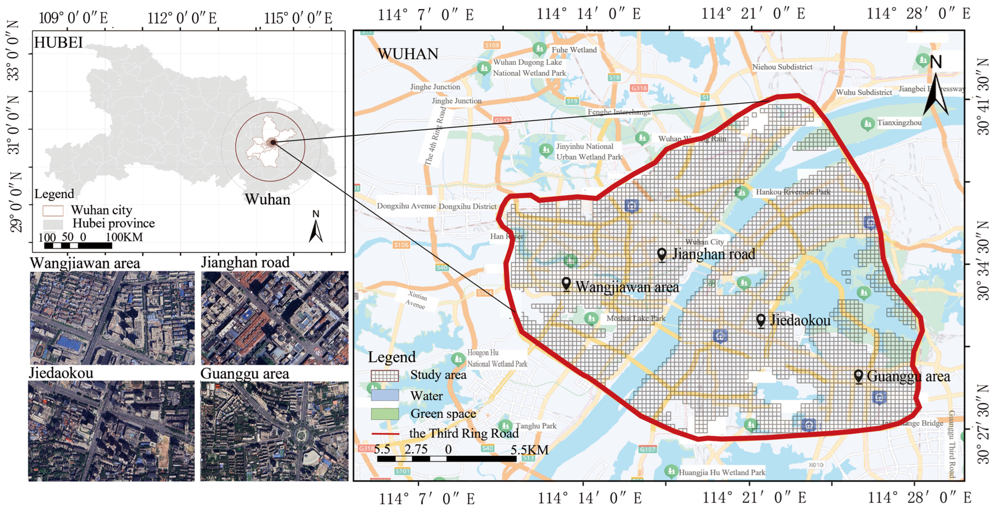
Figure 1. Study area of Wuhan (The base map is sourced from Baidu Maps (https://map.baidu.com/). The satellite imagery overlaying the map is from Google Earth (https://www.google.com/maps/)).
Land 14 02427 g001
Figure 2. Spatial distribution map of SVI classification along the Third Ring Expressway of Wuhan City: (a) Winter; (b) Summer. (All the base images are from Baidu Maps: https://map.baidu.com/).
Land 14 02427 g002
Figure 3. The box plot of the regression coefficient β normalized by z-score: (a) winter; (b) summer.
Land 14 02427 g003
Figure 4. The spatial distribution map of the regression coefficient β of the GWR of each indicator in Winter: (a) W-LST; (b) NDVI01; (c) CaterPOI; (d) TransPOI (e) SportsPOI; (f) ComPOI; (g) ShopPOI; (h) BD; (i) FAR; (j) NDP; (k) NDW; (l) NDS. (All the base images are from publicly accessible online mapping resources: https://map.baidu.com/).
Land 14 02427 g004
Figure 5. The spatial distribution map of the regression coefficient β of the GWR of each indicator in Summer: (a) S-LST; (b) NDVI07; (c) CaterPOI; (d) TransPOI; (e) SportsPOI; (f) ComPOI; (g) ShopPOI; (h) BD; (i) FAR; (j) NDP; (k) NDW; (l) NDS. (All the base images are from Baidu Maps: https://map.baidu.com/).
Land 14 02427 g005
Figure 6. Spatial distribution of urban dynamic vitality (DVSD) across different time slots on rest days: (a) 6:00; (b) 9:00; (c) 12:00; (d) 15:00; (e) 18:00; (f) 21:00. (All the base images are from Baidu Maps: https://map.baidu.com/).
Land 14 02427 g006
Figure 7. Spatial distribution of urban dynamic vitality (DVSD) across different time slots on weekdays: (a) 6:00; (b) 9:00; (c) 12:00; (d) 15:00; (e) 18:00; (f) 21:00. (All the base images are from Baidu Maps: https://map.baidu.com/).
Land 14 02427 g007
Figure 8. Temporal Dynamics of VFI for DVCs: (a) RDVC-1; (b) WDVC-1; (c) RDVC-2; (d) WDVC-2; (e) RDVC-3; (f) WDVC-3.
Land 14 02427 g008
Figure 9. Boxplots of z-score Standardized GWLR Coefficients (β) for the Effects of Three Categories of Influencing Factors on DVC Formation: (a) RDVC-1; (b) WDVC-1.
Land 14 02427 g009
Figure 10. Boxplots of z-score Standardized GWLR Coefficients (β) for the Effects of Three Categories of Influencing Factors on DVCs Formation: (a) RDVC-2; (b) WDVC-2.
Land 14 02427 g010
Figure 11. Boxplots of z-score Standardized GWLR (β) Coefficients for the Effects of Three Categories of Influencing Factors on DVCs Formation: (a) RDVC-3; (b) WDVC-3.
Land 14 02427 g011
Table 1. Description of Evaluation Indicators.
CategoryIndicator (Abbreviation)Calculation MethodUnitSource
Natural Environment
Source:
NASA LAADS DAAC (https://ladsweb.modaps.eosdis.nasa.gov/) (accessed on 25 December 2019)
Winter Land Surface Temperature (W-LST) LST   =   i = 1 n T i n
T i : Land surface temperature of the i-th pixel
n : Number of pixels in the grid
°C[62,63]
Summer Land Surface Temperature (S-LST)°C
Natural Environment
Source:
Landsat 8 OLI, spatial resolution (http://www.usgs.gov/) (accessed on 25 December 2019)
Winter Normalized Difference Vegetation Index (NDVI-01) NDVI   =   NIR   -   RED NIR   +   RED
NIR : Near-infrared reflectance
RED : Red reflectance Travel Purpose
Unitless[64]
Summer Normalized Difference Vegetation Index (NDVI-07)Unitless
Travel Purpose
Source: Amap (https://www.amap.com) (accessed on 24 December 2019)
and Open Street Map (https://www.openstreetmap.org/) (accessed on 24 December 2019)
Catering POI (CaterPOI) POI   =   i = 1 n POI i n
PO I i : The i-th POI for a specific category
n : Number of POI in the grid.
POI/km2[65,66]
Transportation POI (TransPOI)POI/km2
Sports POIPOI/km2
Company POI (ComPOI)POI/km2
Shopping POI (ShopPOI)POI/km2
Built Environment
Source:
Baidu Map (https://lbsyun.baidu.com/) (accessed on 24 December 2019)
Building Density (BD) BD   =   i = 1 n A i A total
A i : Area of the i-th building
A total : Total area of the grid.
%[63]
Floor Area Ratio (FAR) FAR i   =   A i building A i land
A i building : The total building area in grid i
A i land : The land area in grid i ,
Unitless
Distance to Park (NDP) NDP   =   min ( Distance ( P , i ) )
P : Park location
i : Points within the grid.
m[67]
Distance to Waterbody (NDW) NDW   =   min ( Distance ( W , i ) )
W : Waterbody location
i : Points within the grid.
m[68]
Distance to Subway (NDS) NDS   =   min ( Distance ( S , i ) )
S : Subway station location
i : Points within the grid.
m[69]
Table 2. Classification of Steady-State Vitality Zones.
LevelSteady-State Vitality ZoneValue Range
Level 1Low Vitality Zone0–0.042
Level 2Relatively Low Vitality Zone0.042–0.112
Level 3Moderate Vitality Zone0.112–0.204
Level 4Relatively High Vitality Zone0.204–0.356
Level 5High Vitality Core Zone0.356–1.000
Table 3. Classification of Dynamic Vitality Zones.
LevelDynamic Vitality ZoneValue Range (per/km2)
Level 1Low Vitality Zone0–97
Level 2Relatively Low Vitality Zone97–269
Level 3Moderate Vitality Zone269–442
Level 4Relatively High Vitality Zone442–647
Level 5High Vitality Core Zone647–1127
Table 4. Description of Dynamic Vitality Patterns.
DVCTemporal CharacteristicsFigure
RDVC-1/WDVC-1The VFI values on both working days and rest days remain consistently high, thereby demonstrating the characteristic of continuous population aggregationFigure 8a RDVC-1; Figure 8b WDVC-1
RDVC-2On rest days, VFI amplitude > 1.5σ, indicating significant crowd fluctuationsFigure 8c RDVC-2
WDVC-2On weekdays VFI standard deviation < 0.3, indicating relatively stable crowd fluctuations within specific areasFigure 8d WDVC-2
RDVC-3/WDVC-3crowd changes exhibit pronounced bimodal fluctuationsFigure 8e RDVC-3; Figure 8f WDVC-3
Disclaimer/Publisher’s Note: The statements, opinions and data contained in all publications are solely those of the individual author(s) and contributor(s) and not of MDPI and/or the editor(s). MDPI and/or the editor(s) disclaim responsibility for any injury to people or property resulting from any ideas, methods, instructions or products referred to in the content.