Article

Unraveling Socio-Ecological Inequities in Outer London: Cluster-Based Resilience Planning

1
Department of Landscape Architecture, College of Architecture, Planning & Landscape, Newcastle University, Newcastle NE1 7RU, UK
2
Faculty of Forestry, University of British Columbia, Vancouver, BC V6T 1Z4, Canada
*
Author to whom correspondence should be addressed.
Land 2025, 14(12), 2303; https://doi.org/10.3390/land14122303 (registering DOI)
Submission received: 26 October 2025 / Revised: 19 November 2025 / Accepted: 21 November 2025 / Published: 23 November 2025

Abstract

The sustainable development of cities urgently requires an understanding of the interaction between social equity and ecological quality, especially in the peri-urban areas that traditional environmental justice research has paid less attention to. Taking Outer London as an example in this study, the Comprehensive Social Equity Index (CSEI) and the Remote Sensing Ecological Index (RSEI) were constructed to explore the social–ecological coupling relationship and spatial heterogeneity. Four types of socio-ecological coupling were identified through the four-quadrant model, ordinary least squares (OLS), and multi-scale geographically weighted regression (MGWR). The results reveal the characteristics of nonlinear coupling: in addition to the dual disadvantages and advantages of society and ecology, there are also regional patterns where social conditions are advantageous, but ecology is degraded, and where society is weak, but ecology is rich. This indicates that there is a complex spatial dislocation relationship between society and ecology in the peri-urban. The research proposes a scale-sensitive governance strategy based on location, emphasizing the coordinated countermeasures of social reinvestment and ecological restoration, providing a new perspective for environmental justice and sustainable planning in the peri-urban areas of the UK.

1. Introduction

Social and ecological inequity has become one of the core challenges in contemporary urban research, reflecting the uneven distribution of ecological and social resources [1,2]. An increasing number of studies emphasize that opportunities to access ecological resources such as green spaces, environmental quality, and climate resilience are not equally distributed, but are often allocated based on socioeconomic factors such as income, education, and race [3,4,5]. Traditional research on environmental justice has effectively revealed the uneven distribution of environmental hazards in vulnerable communities and put forward the core question of “who is bearing the environmental burden”. It identifies the dual social and environmental burdens faced by marginalized populations [6]. However, this classic perspective gradually reveals its limitations when examining the complexity of contemporary cities. It often focuses on the allocation of environmental disadvantages, but relatively neglects the fairness of access to environmental advantages such as green spaces, ecological services, infrastructure, and fails to fully explain the deep mechanisms of the spatial interaction and dynamic reinforcement between social disadvantages and ecological disadvantages [7].
From a spatial perspective, most environmental justice research focuses on urban central areas, while the peri-urban areas located in the transitional zone between urban and rural areas receive relatively less attention [8]. In Europe, peri-urban areas face complex challenges arising from fragmented governance, mixed land uses, and uneven provision of social services, often resulting in unique patterns of socio-ecological inequity [9]. For example, residents in peri-urban areas may have fewer opportunities to access high-quality ecological resources despite being closer to green infrastructure [10].
To address this gap, this study first distinguishes key concepts that are easily confused in the literature. The concept of inequity is divided into two dimensions: horizontal inequity and vertical inequity. Horizontal inequity emphasizes formal equity and advocates for equal treatment and resource allocation for those with similar or identical situations. Vertical inequity, on the other hand, pursues substantive justice by acknowledging significant differences and inequity between individuals or groups [11]. Therefore, it emphasizes providing differentiated resources to individuals or groups that are proportional to their needs or vulnerabilities [12]. This study adopts the concept of vertical equity because we focus on the disparities between different socio-economic groups. Based on this concept, we further clarified the concepts of social equity and environmental equity, as well as their coupling relationship. Social equity generally emphasizes the fairness of opportunity and resource allocation, ensuring that different social groups can obtain equal development conditions [13]. In the field of the environment, this fairness is reflected in environmental justice, which means the fair distribution of environmental benefits and burdens among communities, allowing everyone to enjoy an equal environment [14]. In addition, ecological quality refers to the physical and biological properties of the environment and is an important indicator of the level of environmental health and the ability to support human and ecosystem needs [15,16]. Overall, social equity and ecological quality constitute the core dimensions of urban social sustainability and environmental sustainability, respectively. Both factors jointly determine the livability and fairness of a city [17,18].
Based on the above background, this study aims to integrate social and ecological indicators to construct a social–ecological framework and analyze the complex inequities in the peri-urban environment. The complex social nature and functional attributes of Outer London provide an ideal research site for studying how society and ecosystems interact spatially. Therefore, the research question of this study is:
(1)
How to construct CSEI and RSEI and systematically incorporate them into the framework of social ecological inequity?
(2)
What is the spatial pattern of social and ecological inequity in Outer London? How do these patterns interact in the peri-urban environment?
(3)
What is the internal mechanism of the social–ecological coupling type?
(4)
How do multi-scale governance approaches correspond to different types of spatial coupling?

2. Methods

2.1. Study Area

This study focuses on 3028 Lower Super Output Areas (LSOAs) within Outer London (Figure 1), each with an average population of approximately 1700 residents [19]. Peri-urban zones are characterized by heterogeneous land uses, socio-demographic diversity, fragmented governance structures, and the coexistence of urban and rural attributes [20,21]. Outer London exemplifies these attributes in multiple ways. First, it displays significant land use heterogeneity, encompassing dense residential zones, commercial hubs, industrial estates, residual agricultural land, and extensive green belts [10,22]. Second, it exhibits socio-economic heterogeneity, with a mixture of affluent communities and marginalized poor communities [23]. Third, the area experiences ecological pressures typical of peri-urban environments [24]. Compared to Inner London, its residents may be closer to ecological resources, but barriers related to accessibility, affordability, and uneven spatial distribution barriers have created new forms of inequity [25]. These features justify the selection of Outer London as a peri-urban case study, providing a suitable reference for exploring social and ecological inequities beyond the city center.

2.2. Research Flow

The research workflow is depicted in Figure 2. The workflow of this study is divided into five main parts. First, socio-economic data were collected from the 2021 UK Census [26]. Data on green spaces were obtained from the Ordnance Survey (OS) Open Greenspace dataset released in 2023 [27], while remote sensing images were obtained from the USGS [28]. Second, two composite indices were constructed: the Composite Social Equity Index (CSEI) and the Remote Sensing Ecological Index (RSEI). In the third step, both CSEI and RSEI were dichotomized using the median-split and natural breaks (Jenks) classification methods. Their combinations generated a 2 × 2 matrix of spatial coupling types representing distinct social–ecological configurations. The fourth stage employed OLS and MGWR to capture the spatial heterogeneity and multi-scalar effects of key determinants influencing ecological quality. Finally, identify the main driving factors and intervention scales, and propose cross-scale differentiated governance strategies.

2.3. Indicator Framework and Construction Rationale

To systematically assess the social and ecological dimensions, this study employs a dual-index framework comprising the Composite Social Equity Index (CSEI) and the Remote Sensing Ecological Index (RSEI). The CSEI emphasizes residents’ access to social resources, while the RSEI emphasizes ecological quality based on remote sensing. A key design principle of these indices is to ensure conceptual distinction and interpretability.

2.3.1. Independent Variables: Composite Social Equity Index

The selection of social indicators for CSEI is based on the existing theoretical and policy frameworks in the UK, which aim to address multidimensional poverty and social inclusion issues in the country. We draw inspiration from Townsend’s concept of poverty (IMD) and the Social Mobility Framework of the Social Mobility Commission. Conceptualize social equity as encompassing multiple dimensions such as education, economy, health, housing, and culture [29,30]. Therefore, the selection of each indicator is not only based on the availability of data, but also on its theoretical connection with the recognized determinants of fairness in UK urban policies. Specifically, education and employment reflect human capital and opportunity structure [30,31], while housing ownership and overcrowding reflect opportunities for wealth accumulation and stable living conditions [32]. Health and crime indicators represent community well-being and social cohesion [33]. The accessibility of green spaces follows the perspective of environmental justice, where equitable access to natural resources is a key component of urban equity [34]. Finally, language barriers and ethnic diversity are also considered to reflect cultural inclusivity and social participation, particularly in the multiethnic peri-urban areas of London [35]. These indicators are consistent with the seven domains of the IMD, ensuring that the constructed index reflects both theoretical rigor and policy relevance. In addition, we have provided clear definitions for the direction of each indicator based on relevant research in the UK context.
It is worth noting that green space accessibility is included in CSEI as an indicator of social service accessibility, representing residents’ ability to access public amenities [36]. In terms of calculation, the Euclidean distance method was used to estimate the total area of all green spaces within a 1000 m radius of each LSOA centroid [37]. In addition, ethnic diversity reflects the unique socio-cultural structure of the peri-urban areas of London. In the UK, cultural diversity has a dual nature: on the one hand, it promotes cross-cultural exchange; on the other hand, it may also be accompanied by structural inequality, leading to the concentration of ethnic minorities in areas of poverty or harsh environments [38]. Therefore, ethnic diversity in this study does not represent a denial of diversity itself but is seen as a reflection of spatially concentrated disadvantages [39].
The weighting of the indicators is a key methodological decision. This study adopts a multidimensional approach to balance interpretability and statistical robustness. First, to address potential redundancy among the selected social indicators, a Spearman correlation analysis was performed on all eleven variables, examining indicators with |ρ| > 0.8 [40]. To reduce multicollinearity and preserve the potential structure of the data, we use principal component analysis (PCA) to perform dimensionality reduction on highly correlated indicators. Subsequently, the comprehensive indicators obtained from PCA were included in the weighting process along with other independent variables to construct the CSEI [41]. The weighting method employed is the Entropy Weight Method (EWM).

2.3.2. Dependent Variables: Remote Sensing Ecological Index (RSEI)

Landsat remote sensing images used in this study were obtained from the United States Geological Survey (USGS). We selected a Landsat 8 (OLI/TIRS) scene acquired on 7 September 2023 due to its complete spatial coverage and minimal cloud contamination, ensuring high-quality data acquisition. Its temporal proximity to the 2021 Census further enhances the comparability between social and ecological indicators. The RSEI consists of four indicators: NDVI, WET, LST, and NDBSI, representing greenness, humidity, heat and dryness, respectively [42]. These four indices are closely related to ecological quality. Their contributions to RSEI are determined by the inherent statistical characteristics of the data rather than by human-defined subjective weighting, thereby enhancing objectivity [43]. Normalized Difference Vegetation Index (NDVI) is used to measure the state of vegetation. Higher NDVI values indicate denser, healthier plant cover [44]. The wet index is closely related to the humidity of vegetation and soil, and its value is used to reflect the humidity status in the study area [45]. Land surface temperature (LST) is used to represent heat. The dryness index is expressed using the NDBSI, which is combination of the Index-based Built-up Index (IBI) and the soil index (SI) [44]. The detailed calculation formula is shown in Table A1.

2.4. Spatial Cluster Analysis

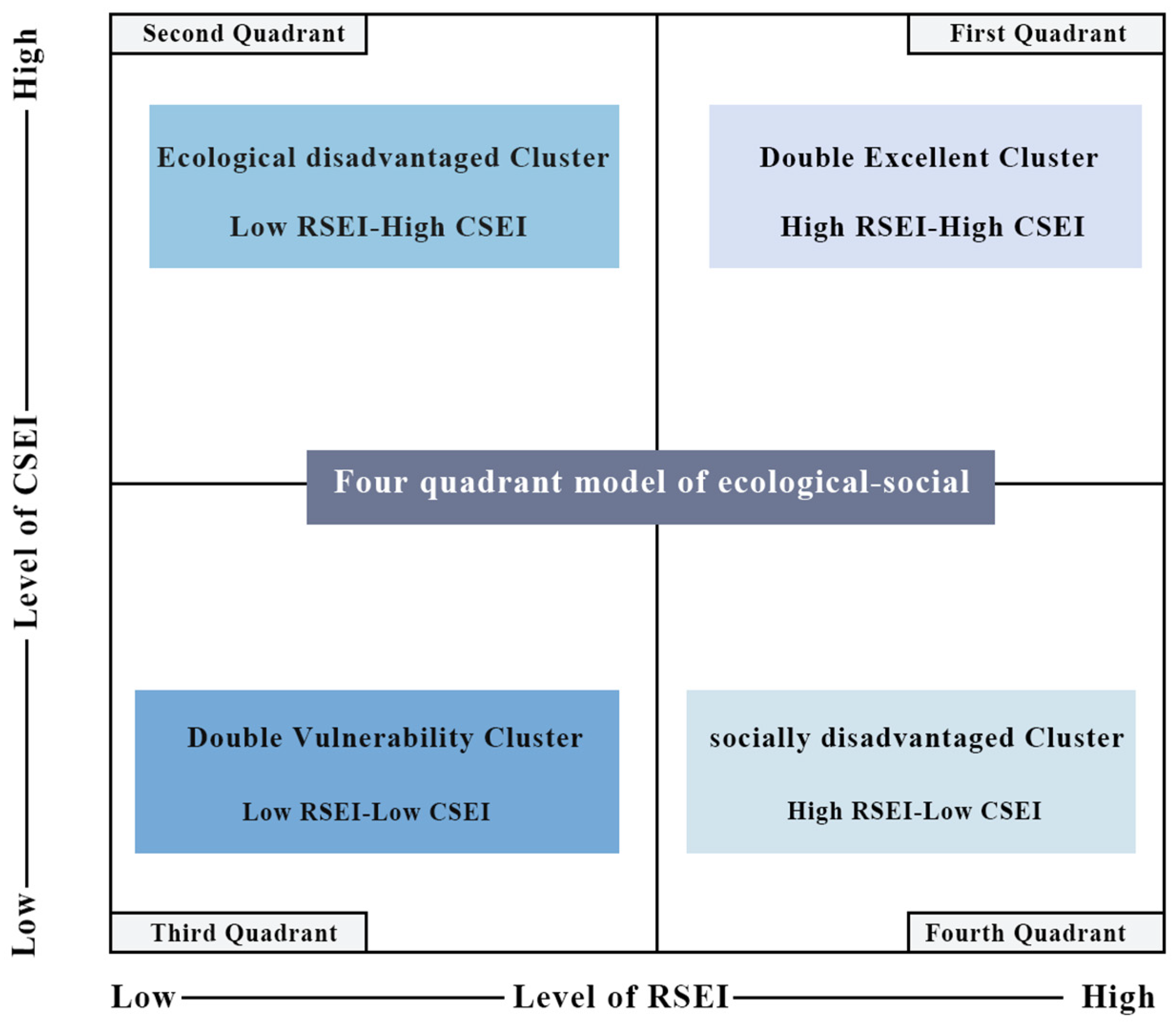
To identify the interaction patterns between social inequity and ecological quality, this study classified and spatially clustered the CSEI and the RSEI. This study used a four quadrant classification method to divide these two indicators into high and low groups [46]. The RSEI was classified using the Jenks natural breaks method to capture the natural spatial gradients of ecological quality, while the CSEI was classified using the median threshold to ensure comparability across time and regions [47,48,49]. This mixed approach balances the ecological realism of RSEI with the statistical consistency of CSEI, a strategy also adopted in recent socio-ecological equity studies [50,51]. Ultimately, all LSOAs were categorized into four types: High RSEI-High CSEI is a double excellent cluster, indicating that both the social equity index and ecological quality are relatively high, demonstrating the characteristics of the synergy between society and ecology. Low RSEI-Low CSEI represents a double vulnerability cluster, indicating that ecological degradation and social inequity in this area intensify each other. Therefore, “ vulnerability “ describes the mutually reinforcing disadvantages, while “excellence” reflects the mutually reinforcing advantages [52,53]. High RSEI-Low CSEI, indicating good ecological conditions but serious social inequity, defined as an ecologically disadvantaged cluster (Figure 3). This typology echoes the emerging research on urban environmental justice, emphasizing that social and ecological differences are not always spatially consistent [54].

2.5. Ordinary Least Squares (OLS)

The OLS model was applied to examine the global relationship between RSEI and CSEI. OLS is a widely used linear regression technique for assessing the correlation between independent and dependent variables. In this study, the model was used to explore the relationships between nine social variables and the RSEI. To assess potential multicollinearity among variables, the variance inflation factor (VIF) was calculated for each explanatory variable [55]. Prior to the regression analysis, all variables were standardized using the z-score method. The detailed calculation formula is shown in Table A2.

2.6. MGWR Analysis

Since the OLS model neglects spatial heterogeneity, the influence of CSEI on RSEI may vary across different parts of Outer London. This study uses MGWR to examine the geographical differences in the relationship between the dependent variable and the independent variable. The traditional GWR assumes that all variables have the same spatial influence range, which may lead to overfitting or underfitting of the model. In contrast, MGWR allows each explanatory variable to have different spatial scales, that is, bandwidth, and determines an independent spatial heterogeneity scale for each variable, which is suitable for analyzing the influence of different social factors at different spatial scales [56,57]. The detailed calculation formula is shown in Table A2.

3. Results

3.1. Results of Spearman Correlation

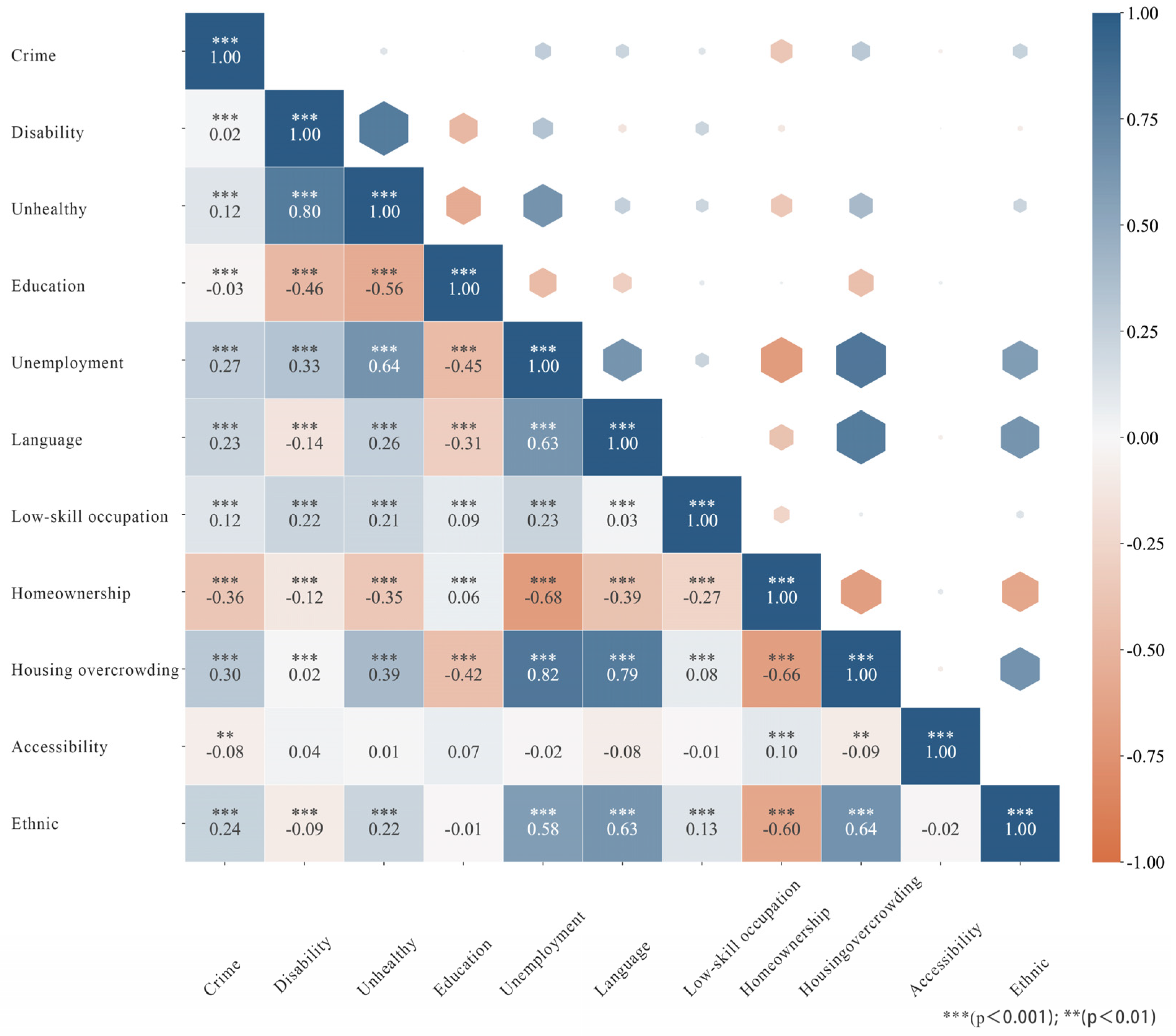
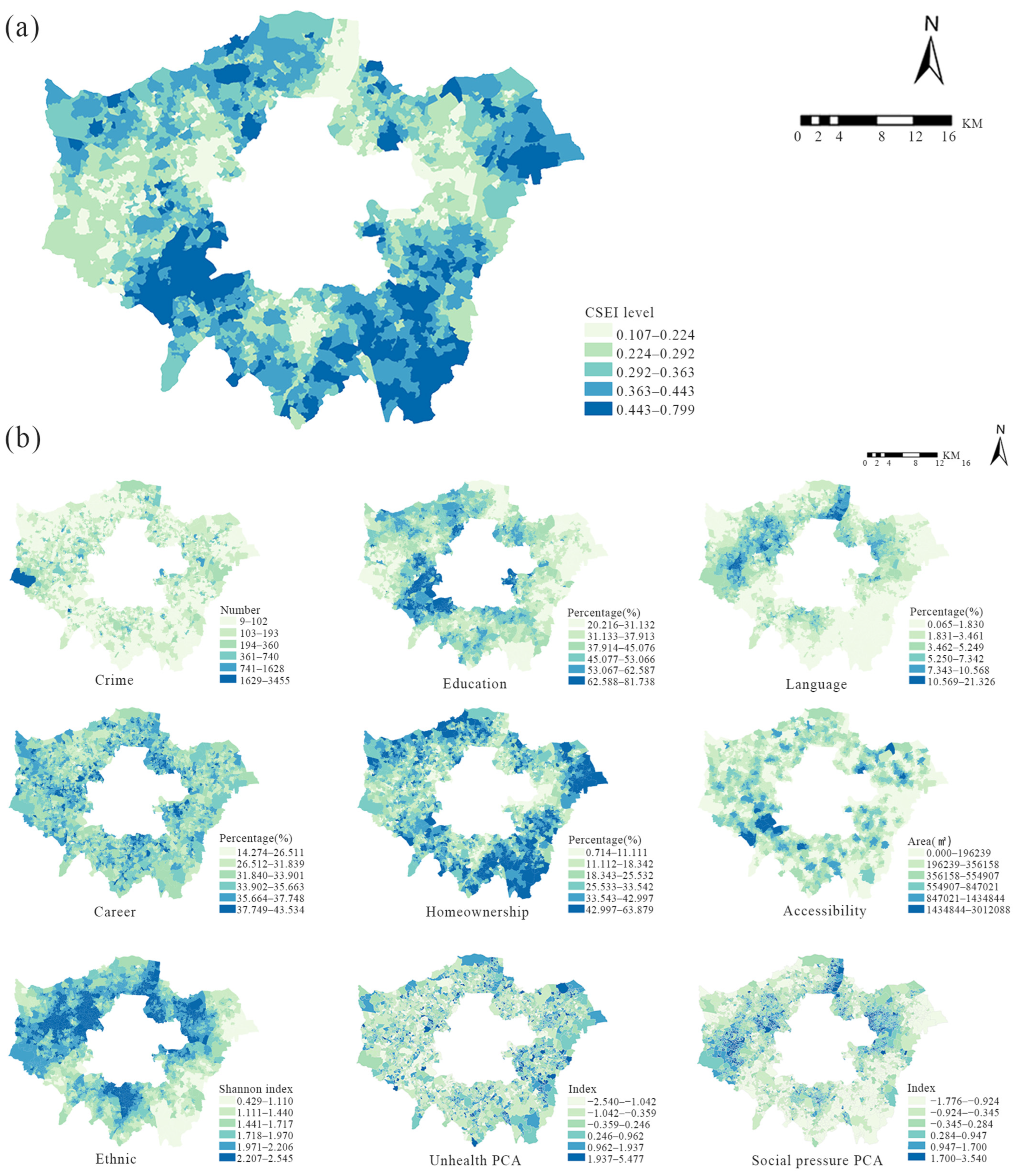
The Spearman correlation analysis results are shown in Figure 4. The heatmap represents the correlation between 11 variables. Overall, most variables exhibit weak to moderate correlation. However, two pairs of indicators showed a strong correlation: unhealthy rate and disability rate (ρ = 0.80, p < 0.001), as well as unemployment rate and housing crowding rate (ρ = 0.82, p < 0.001). These high correlations indicate potential redundancy, and to reduce multicollinearity while preserving potential information structures, PCA is performed on highly correlated indicators [41]. The final weight results and original dimensions are shown in Table 1. The distribution maps of various socio-economic variables and CSEI are shown in Figure 5.

3.2. The RSEI of Outer London

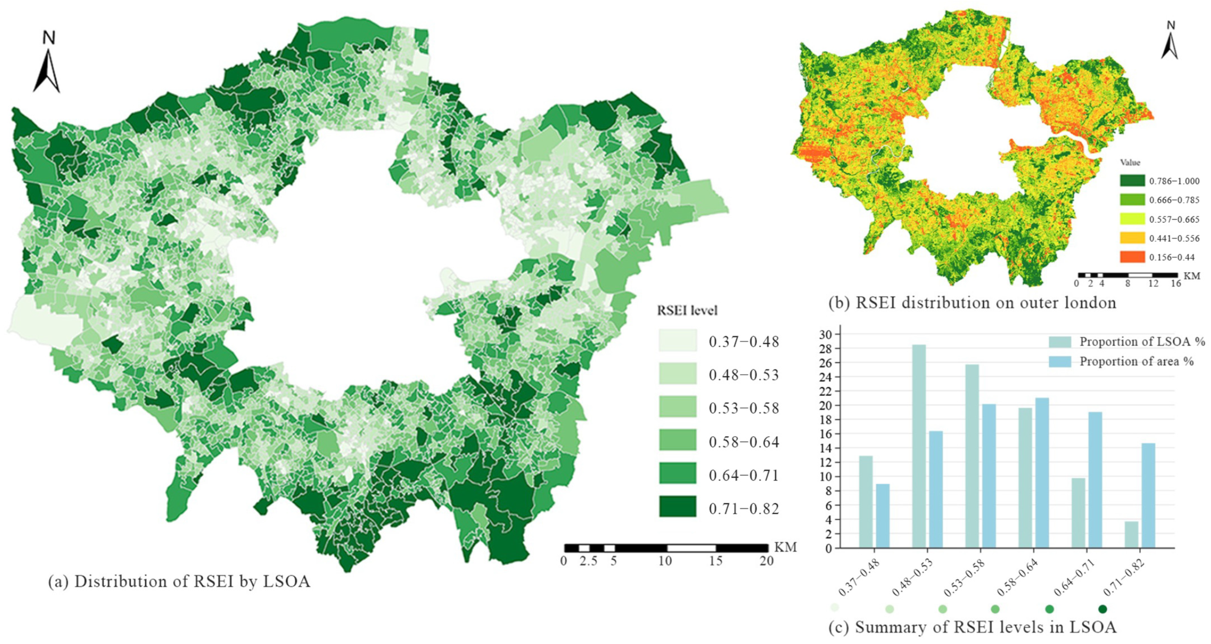
Figure 6 shows the spatial distribution characteristics of the overall ecological quality of Outer London. To clarify the specific ecological quality of each LSOA and reveal significant ecological differences between regions, we calculated the average RSEI values of each LSOA. As shown in Figure 6. The overall ecological quality presents a pattern of high outside and low inside. The areas with higher ecological quality are mainly located in the peripheral areas of Outer London, which are closely connected to the green belt areas. This pattern aligns with evidence from London that its Green Belt functions not only as a boundary to urban expansion but also preserves elevated landscape and ecological quality compared to the city core [58].

3.3. The Relationships and the Spatial Disparities Between CSEI and RSEI

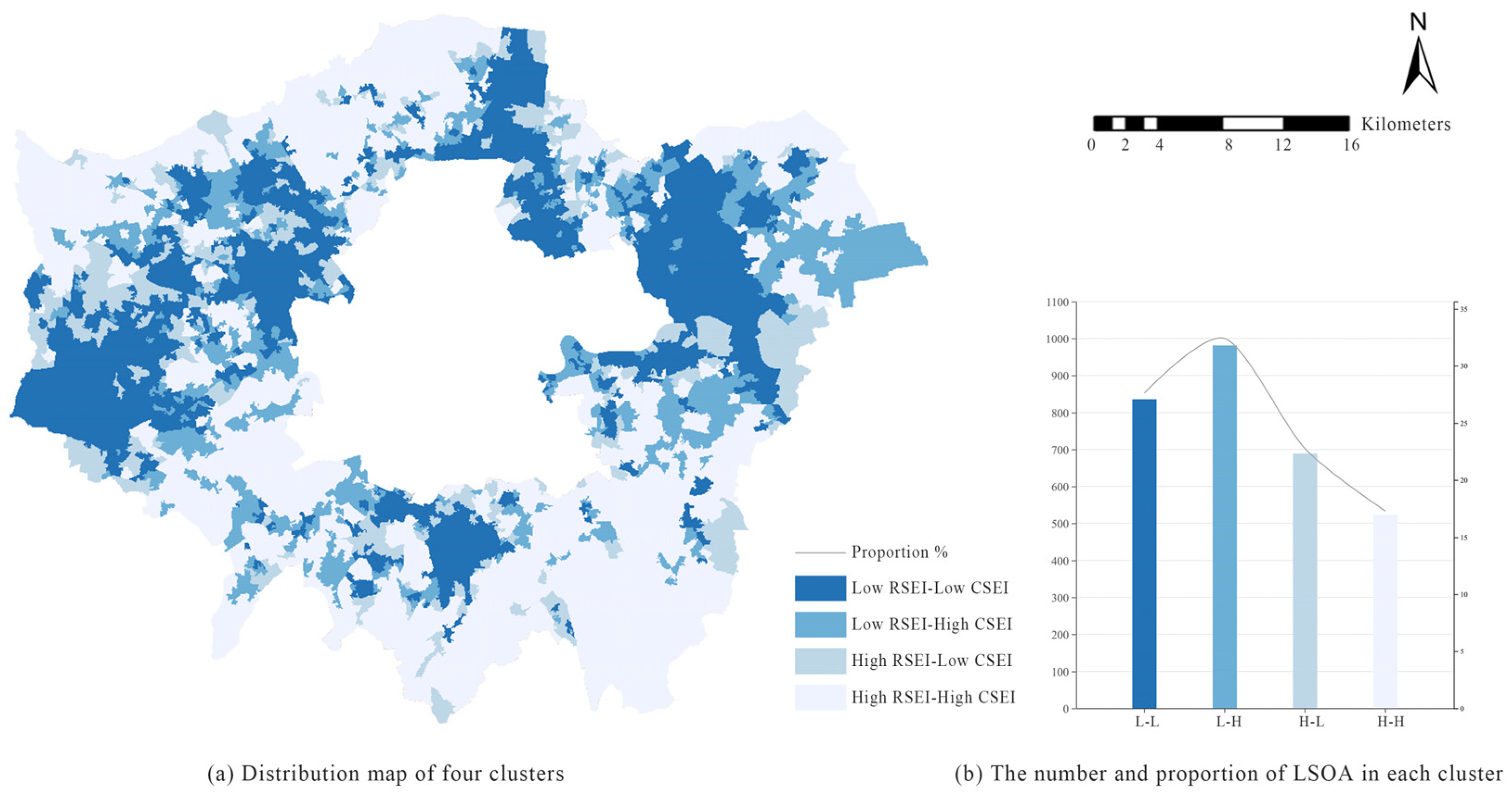
According to the RSEI and CSEI analysis of Outer London, Figure 7 shows the distribution of four different spatial types in Outer London. Among them, 27.58% of the regions belong to the category of Low RSEI-Low CSEI, representing regions with equally poor socio-economic levels and ecological quality. These regions are mainly distributed in the west and east. 32.40% of the Outer London area is classified as an Ecological Disadvantaged Cluster, characterized by Low RSEI-High CSEI. In contrast, 17.27% of the regions belong to the High RSEI-High CSEI category, known as the Double Excellent Cluster. It is mainly distributed in Richmond upon Thames, Barnet, and Bromley. Finally, 22.75% of the Outer London area is classified as High RSEI-Low CSEI, representing areas with relatively good ecological quality but low social equity, mainly distributed in peripheral areas.

3.4. OLS Result

The OLS results showed that CSEI had a significant positive impact on RSEI (β = 0.425119, p < 0.01), indicating that the higher the degree of social equity in a region, the better its ecological quality. In terms of specific social indicators, it was found that the number of crimes, the rate of language barriers, racial diversity and social pressure have significant negative effects on RSEI. Homeownership rate, higher education rate and accessibility have a positive effect on RSEI. It is worth noting that unhealthy levels and the rate of low-skilled occupations also have a positive effect on RSEI (Table 2).

3.5. Spatial Agglomeration Analysis

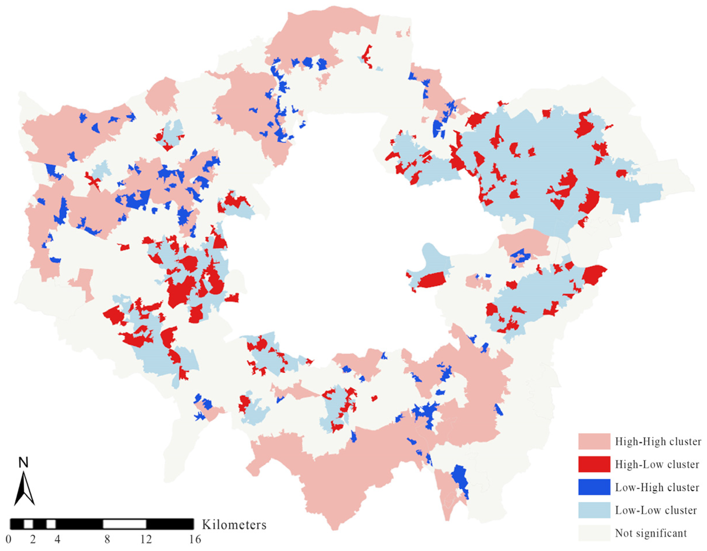
After OLS analysis, Moran’s I calculation is performed on the residuals of the OLS model to evaluate its adaptability(Figure 8). The results showed significant spatial autocorrelation in the residuals (Moran’s I = 0.31, p < 0.01), indicating that the OLS model failed to fully explain spatial differences and local regression methods need to be introduced [57].

3.6. Model Comparison

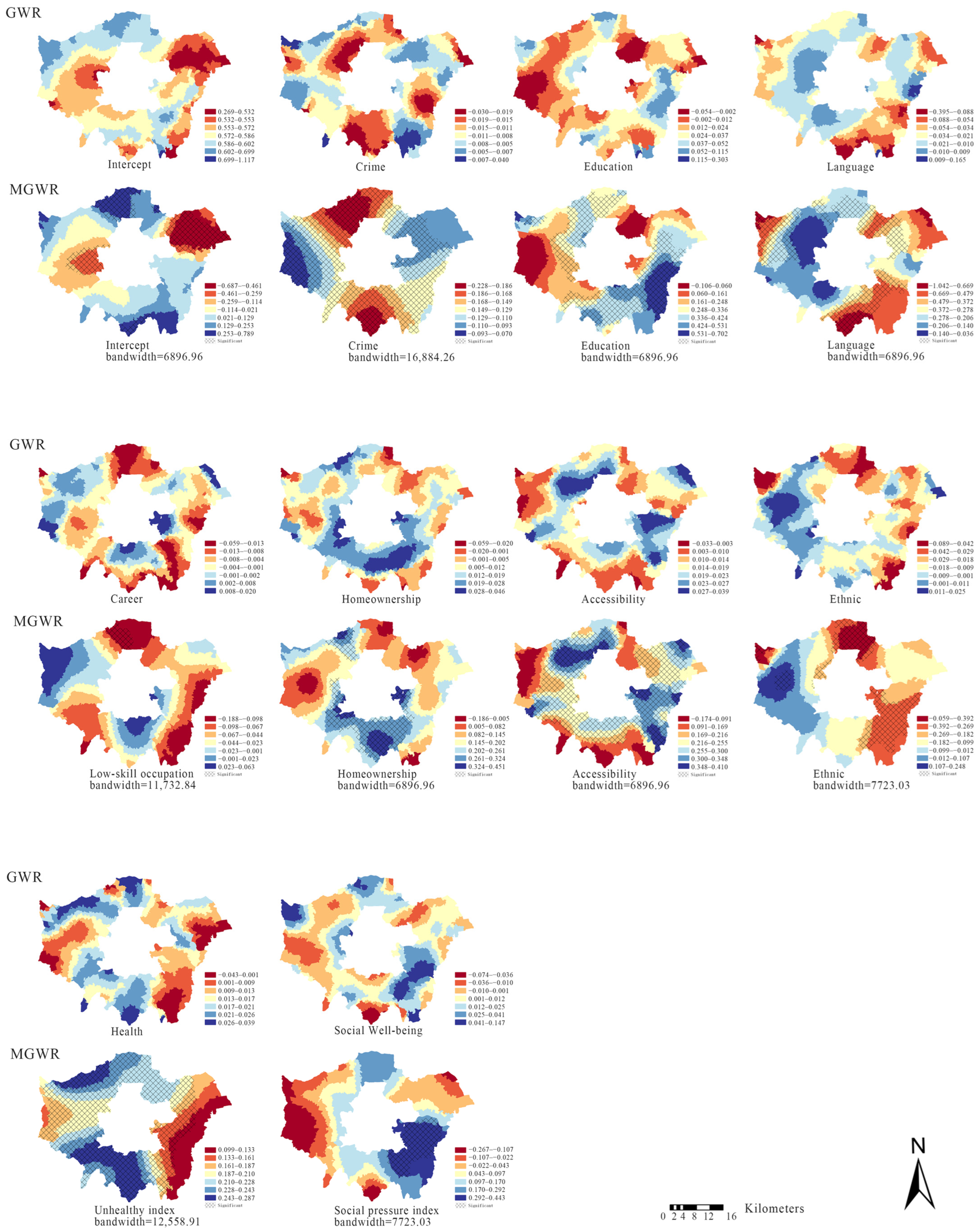
This study constructed GWR and MGWR models using the same variables as the OLS model to explore the spatial heterogeneity of the relationship between CSEI and RSEI. Compared with the GWR model, MGWR outperforms GWR in terms of fitting goodness and residual independence, with an adjusted R2 of 0.5994 and a significant decrease in AICc to 5999.2276. This indicates that MGWR can better reveal the multi-scale spatial mechanisms of social ecological relationships. The comparison results of the models in Table 3 show that there are differences between the results of GWR and MGWR. The intercept range in the GWR model is from 0.2691 to 1.1172, while the intercept range observed in the MGWR model is from −0.6871 to 0.7893. Figure 9 compares the results of GWR model and MGWR model. The spatial distribution trends of GWR and MGWR are roughly similar, but there are differences. The coefficient spatial distribution transition of MGWR is smoother, indicating that its spatial pattern is more stable. In contrast, the spatial variability of GWR is more pronounced, and the transitions between regions are more intense. This is because MGWR uses adaptive bandwidth for each variable, allowing for a more detailed analysis of spatial heterogeneity and capturing significant areas that GWR may not be able to recognize.
In terms of coefficient spatial distribution, the standard deviation of ethnic diversity is the largest, followed by the higher education rate and the language barrier rate, indicating significant spatial differences in the impact of these variables on RSEI. The intercept represents the predicted value of the dependent variable when all independent variables are zero, reflecting the relationship between different locations and RSEI in this analysis. The results showed a significant positive correlation between most regions and intercepts, with only some regions in the east and west showing a negative correlation.
Previous studies have shown that urban greening often benefits high-income and highly skilled individuals, a phenomenon known as green gentrification [59]. Such processes usually lead to a close spatial integration of high ecological quality and socio-economic privileges. Interestingly, our MGWR results indicate that in Outer London, there are fewer significant regions for the low-skilled occupation variable, suggesting a relatively weak relationship between this variable and the RSEI within the study area. This deviation from the typical green gentrification model may be attributed to the characteristics of peri-urban areas, such as the presence of green belts, lower housing costs, and historical planning policies for protecting green Spaces without evicting low-skilled populations [60]. In addition, both the unhealthy index and social pressure demonstrate positive spatial relationships with RSEI across most parts of Outer London. This pattern suggests that in some cases, higher ecological quality does not necessarily coincide with better social conditions. By capturing such multi-scale characteristics, MGWR can more accurately reflect the heterogeneous effects of different variables on the four clusters. The multi-scale results thus provide an empirical basis for proposing targeted and localized intervention strategies.

4. Discussion

4.1. Differentiated Drivers of Socio-Ecological Patterns

This study reveals a pronounced spatial mismatch between social equity and ecological quality across Outer London. Unlike studies that mainly focus on the central urban [61,62], the peri-urban context of Outer London amplifies the complexity of socio–ecological coupling and challenges the conventional assumption that social disadvantage necessarily coincides with environmental disadvantage [63]. At the same time, we also recognize another viewpoint: peri-urban areas usually have more open land than central urban areas, which in principle may provide greater space for the creation of new green spaces. However, the availability of land itself does not guarantee that it can be directly transformed into usable and publicly accessible green spaces. In the context of the UK, many peri-urban lands are restricted by green belt policies, land use planning and scattered private property rights. These factors impose legal and practical restrictions on reconstruction, making planning permission, land integration and management complex [10,64]. This increases the coordination cost of inclusive intervention measures. Therefore, although the stock of peri-urban land can be used as a green resource, achieving fair social and ecological benefits usually requires multi-level and cross-departmental governance, rather than relying solely on land availability.
The MGWR results in Table 4 reveal different but interrelated mechanisms among the four clusters. Among all the clusters, the most consistent finding is the strong negative impact of language barrier rates, which contrasts sharply with the positive effects of higher education rates and green accessibility.
In the Low RSEI–Low CSEI cluster, mainly concentrated in Barking and Dagenham, southern Hillingdon, and Brent, the most influential variable is the language barrier rate, showing a significant negative association. This indicates that language isolation fundamentally restricts both social participation and equitable access to ecological environments, exacerbating the disadvantages faced by ethnically diverse and low-income communities [65]. In contrast, higher education and green accessibility exhibit positive effects, suggesting that stronger educational capital and better green infrastructure can partially mitigate poor environmental conditions. This region reflects a dual exposure mechanism in environmental research, where social and ecological vulnerabilities reinforce each other [53]. Therefore, in governance, it is necessary to combine ecological restoration with social inclusiveness.
A similar structure emerged in the Low RSEI-High CSEI cluster, where education was the most positive factor, while language barriers remained a strong negative factor. These ecological disadvantages in social progress reflect the dynamics of green gentrification, that is, social and economic progress outpaces environmental restoration [59,66]. This indicates that environmental inequity does not only affect vulnerable groups. Dominant groups may also be constrained by insufficient ecological space allocation [4]. Green transformation and ecological compensation need to be emphasized in policy intervention.
The High RSEI-Low CSEI clusters are mainly located in the west, characterized by abundant natural assets but persistent socio-economic disparities. This discovery indicates that ecological resources are abundant in space but unavailable in society. This is a potential inequity phenomenon [67]. Evidence within the UK suggests that even with positive green space indicators, impoverished communities still face significant barriers to access. For example, Gant et al. [10] emphasized that peri-urban areas in London exhibit ecological wealth, but due to the imperfect social system, the accessibility of green facilities is fragmented. In addition, it should be emphasized in this study that high RSEI measured by remote sensing does not automatically equate to high-quality urban green spaces or ecological services available for residents to utilize. For example, although natural vegetation on abandoned or reclaimed land increases RSEI, such spaces may lack biodiversity management or active use of communities [68]. Therefore, our interpretation of high RSEI regions should be cautious. When high RSEI is driven by proactive planning and governance, it is more likely to be transformed into social welfare; When high RSEI comes from passive regeneration or divestment, its social benefits are often limited and may mask issues of poverty and infrastructure scarcity. Based on this, policy recommendations for high RSEI low CSEI regions should focus on transforming “ecological capacity” into “socially accessible high-quality green spaces”.
In contrast, in High RSEI-High CSEI clusters, namely dual-excellent districts such as Richmond and Kingston, the educational level and green space accessibility jointly play a key role, forming a virtuous cycle of educational capital and environmental capital [69]. It reflects the bidirectional strengthening effect of social resources and ecological resources and shows the characteristics of balance [52]. However, it should be noted that the continuously rising housing costs and spatial exclusivity may also translate synergies into selective privileges. Therefore, to prevent excessive concentration of ecological capital and social capital, which may lead to regression or new unfair phenomena, governance should not only be adaptive, but also clearly guided by fairness. Specifically, while maintaining fair distribution, dynamically adjust the governance model. It includes monitoring ecological benefits, reinvesting the resulting benefits into low-income communities, and inclusive participation to prevent selective benefits. This is consistent with the adaptive governance theory [70] and equity oriented urban greening research [71], as well as the cross administrative strategic planning principles in the London Plan [72]. Through these adaptable yet fair mechanisms, high benefit areas in the peri-urban areas of London can become a model of social and ecological resilience.

4.2. Unequal Green: Ecological Recovery Amid Social Decline

Although traditional views often interpret ecological improvement as necessarily beneficial, our research findings challenge this hypothesis by revealing that higher RSEI values are consistent with higher levels of social vulnerability, particularly reflected in higher rates of poor health and social pressure. These results are confirmed in the output of MGWR (Table 3). This phenomenon was observed in the High RSEI Low CSEI cluster in this study. This phenomenon may reflect the green divestment effect, where ecological improvement does not stem from active environmental planning, but from market withdrawal, industrial decline, or population decline [73]. This process often occurs during the postindustrial or transitional period of urban development, where deindustrialization, population loss, and land abandonment allow vegetation to spontaneously recover, leading to an increase in RSEI, even if social development stagnates or even declines. Importantly, this dynamic change indicates that the relationship between RSEI and CSEI is influenced by the stage of urban landscape development and land use trajectory. Regions in the early stages of urban expansion often experience ecological degradation with rapid growth, while mature or shrinking regions may demonstrate significant ecological improvement through natural restoration or brownfield succession. This regulatory mechanism has been confirmed in multiple studies [74,75]. Therefore, it is crucial to distinguish between “growth driven” and “divestment driven” greening when interpreting higher RSEI values. Integrating urban development indicators such as land use transformation, population change, or brownfield density can clarify whether ecological improvement translates into real social benefits or vulnerability [75]. Furthermore, this phenomenon may also be related to policy orientation and redistribution systems. Targeted ecological investments by London and local authorities may have prioritized funding to highly vulnerable communities, improving ecological quality in the short term [76].

4.3. Multi-Scale Interpretation and Governance Implications of MGWR

4.3.1. Macro Driving Factors

Crime (bandwidth = 16,884.26), unhealthy index (bandwidth = 12,558.91), and low-skilled occupation (bandwidth = 11,732.84) play a role on a larger spatial scale. They reflect structural and regional influences, such as the labor market, the policing system, and the health conditions of residents. The relatively large bandwidth of the unhealthy index is consistent with the pattern of economic recession and population decline increasing ecological quality on a large scale [77]. These driving factors require cross-regional coordinated intervention measures, such as labor market plans, cross-regional security governance strategies, and planning consistent with greenfield investment policies [78].

4.3.2. Micro Driving Factors

Language barriers (bandwidth 6896.96), social pressure index (bandwidth = 7723.03), and accessibility (bandwidth 6896.96) have shown a strong impact on RSEI, but within a more limited spatial range. The strong negative coefficient of the language barrier rate, combined with a relatively small bandwidth, indicates highly localized social exclusion. The positive and moderate scale effects of green space accessibility indicate that green space strategies such as connectivity and walkable networks are important in local to regional intervention policies. Racial diversity (bandwidth = 7723.03) and social pressure index are also more localized, which means that targeted community communication and assistance policies are needed. These driving factors are best addressed through community-level measures. This regional role is consistent with research indicating that culture and language play a role in finer spatial granularity and regulate environmental access [79].

4.3.3. Multi-Scale Governance Strategy

Based on the results of MGWR and four social ecological clusters, this study emphasizes that social reinvestment must be spatially coordinated with ecological planning to ensure that environmental justice is not only for poverty alleviation, but also for jointly creating ecological and social resilience. Table 5 summarizes the internal mechanisms and corresponding policy interventions of the four spatial types in Outer London. By matching the key variables of each cluster with the corresponding governance hierarchy, this framework transforms spatial diagnosis into actionable strategies. This multi-scale design emphasizes that social ecological justice cannot rely on unified governance policies; On the contrary, it requires scale sensitive adaptive governance that links communities with regional environmental planning to ensure the ecological integrity and social inclusiveness of Outer London. This approach aligns ecological and social strategies with differentiated but complementary goals, guiding targeted interventions towards fairness, resilience, and sustainability [80].

4.4. Global Comparison and International Significance

Comparing the social ecological inequity phenomenon in Outer London within a global framework can help highlight the theoretical value and universal significance of this study. International research has generally found that socially vulnerable groups are more susceptible to environmental risks, such as low-income and minority communities in the United States, often facing multiple disadvantages, including air pollution, lack of green spaces, and climate disasters [6,86]. In Latin American cities, rapid urbanization and informal land use have led to the concentration of poor populations in ecologically fragile areas [87]. In East Asian, the allocation of green spaces and public resources is often deeply coupled with the social hierarchy structure [88]. Compared to these cities, Outer London is characterized by a more complex pattern of inequity in the peri-urban context. Therefore, this study provides three insights for international research: 1. Type diversity. Environmental inequity may manifest as both environmental deprivation by socially disadvantaged groups and a complex state of mismatch between social and ecological resources. 2. Peri-urban dimension. Most international studies focus on urban core areas, while this study emphasizes the social ecological heterogeneity of peri-urban areas, which has universal significance for rapidly expanding cities worldwide. 3. Methodological contributions. This study presents a portable research framework through CSEI-RSEI coupling and MGWR multi-scale diagnosis. It can be applied in different countries and cities to promote cross-border comparative research.

4.5. Limitations and Future Research

Although this study is innovative in theory and methodology, there are still limitations. Firstly, this study is mainly based on single-year data. Although it can effectively depict the social ecological spatial pattern, it limits the observation of the dynamic evolution of the relationship between the two. Urban ecological policies typically have significant time lag effects [89]. Future research needs to use longitudinal research designs, such as multi-period remote sensing monitoring and comparison before and after policy implementation, to capture the dynamic evolution of social ecological systems more deeply and more accurately evaluate the cumulative effects of policy interventions. Secondly, although the indicator system covers the main social and ecological dimensions, it does not include key environmental factors such as air pollution, noise, and climate vulnerability, which may underestimate certain potential risks. Thirdly, using the four-quadrant classification method for spatial classification may be too simplified and unable to classify in a refined manner. Finally, this study uses the remote sensing composite index RSEI to represent the level of ecological quality, which provides the advantage of strong comparability and suitability for large-scale analysis. However, RSEI is mainly based on spectral signals and cannot directly measure other aspects of ecological value such as biodiversity, management quality, and social availability on the ground. Future research may consider combining RSEI with ground biodiversity and residential use data to assess ecological advantages more comprehensively [90].

5. Conclusions

Combined with the MGWR framework, this study constructed the CSEI and RSEI for Outer London to analyze the patterns of social–ecological inequity in the context of peri-urban areas. The results revealed that while social equity and ecological quality are generally positively correlated, the coupling patterns vary across regions, reflecting both the coexistence and misalignment of socio-ecological advantages and disadvantages. This discovery contradicts the single hypothesis in most existing studies that socially disadvantaged groups inevitably bear environmental disadvantages. In terms of methodology, this study developed CSEI and combined it with RSEI to analyze the spatial pattern of the entire Outer London, thereby deepening the understanding of social ecological equity. Spearman analysis, PCA, Entropy weight method, spatial quadrant analysis, and the multidimensional integration method of MGWR jointly reveal the structural and internal mechanisms of peri-urban inequity. In practice, a three-level governance approach has been proposed: 1. Regional policies that address macro driving factors and coordinate cross-regional green investment; 2. Action to integrate housing, education, and green infrastructure planning within the administrative region; 3. Community-level projects aimed at eliminating language and cultural barriers and establishing local management. This differentiation strategy not only aligns the intervention scale with the driving factor scale revealed by MGWR, but also improves target accuracy. At the same time, this strategy also emphasizes the necessity of considering potential social risks. In summary, this study not only deepens the understanding of social ecological inequity in the peri-urban areas of London, but also provides a theoretical and methodological path for international research, which helps to establish a more universal comparative framework for social ecological inequity.

Author Contributions

Conceptualization, Q.M. and M.C.; methodology, Q.M.; software, Q.M.; validation, Q.M. and M.C.; formal analysis, Q.M.; investigation, Q.M. and M.C.; resources, Q.M.; data curation, Q.M.; writing—original draft preparation, Q.M.; writing—review and editing, M.C. and Q.M.; visualization, Q.M.; supervision, M.C.; project administration, M.C. All authors have read and agreed to the published version of the manuscript.

Funding

This research received no external funding.

Data Availability Statement

All main research data are included in this paper.

Conflicts of Interest

The authors declare no conflicts of interest.

Abbreviations

The following abbreviations are used in this manuscript:
CSEIComprehensive Social Equity Index
RSEIRemote Sensing Ecological Index
EWMEntropy Weighting Method
PCAPrincipal Component Analysis
OLSOrdinary Least Squares
MGWRMulti-scale Geographically Weighted Regression
GWRGeographically Weighted Regression
NDVINormalized Difference Vegetation Index
LSTLand surface temperature
IBIIndex-based Built-up Index
SISoil Index

Appendix A

Table A1. Formula and Reference of the four ecological indicators.
IndicatorsFormulaDescriptionExplanation
Greenness N D V I = ρ N I R ρ R e d ρ N I R + ρ R e d Normalized Difference Vegetation Index (NDVI) is used to measure the state of vegetation. Higher NDVI values indicate denser, healthier plant cover.where ρ N I R , ρ R e d represent Landsat 8 OLI/TIRS bands, respectively [44].
Wet W E T = δ 1 ρ B l u e + δ 2 ρ G r e e n + δ 3 ρ R e d + δ 4 ρ N I R + δ 5 ρ S W I R 1 + δ 6 ρ S W I R 2 The wet index is closely related to the humidity of vegetation and soil, and its value is used to reflect the humidity status in the study area.where ρ B l u e , ρ G r e e n , ρ N I R , ρ S W I R 1 ,   ρ S W I R 2 represent Landsat 8 OLI/TIRS bands, respectively. δ i are the calculation coefficient of the humidity component in the K-T transformation of different types of Landsat data [91].
Heat L S T = T B 1 + λ T B ρ l n ( ε )
ρ = h c k
Land surface temperature (LST) is used to represent heat.where T B is the brightness temperature, λ is the band central wavelength, h is the Planck’s constant ( 6.626 × 10 34   J s ), c is the velocity of light (2.998 × 108 m/s) and k is the Boltzmann constant ( 1.38 × 10 23 J / K ) [92].
Dryness N D B S I = S I + I B I 2
S I = ρ S W I R 1 + ρ R e d ρ N I R + ρ B l u e ρ S W I R 1 + ρ R e d + ρ N I R + ρ B l u e
I B I = 2 × ρ S W I R 1 / ( ρ S W I R 1 + ρ N I R ) [ ρ N I R / ( ρ N I R + ρ R e d ) + ρ G r e e n / ( ρ G r e e n + ρ S W I R 1 ) ] 2 × ρ S W I R 1 / ( ρ S W I R 1 + ρ N I R ) + [ ρ N I R / ( ρ N I R + ρ R e d ) + ρ G r e e n / ( ρ G r e e n + ρ S W I R 1 ) ]
The dryness index is expressed using the NDBSI, which is combination of the Index-based Built-up Index (IBI) and the soil index (SI).where ρ i represent the bands of the remote sensing image [44].

Appendix B

Table A2. The calculation formulas of OLS and MGWR.
IndicatorsFormulaExplanation
OLS y = β 0 + i = 1 p   β i x i + ε where y is the dependent variable (RSEI); β 0 represents the intercept term; β i is the estimated coefficients; x i represents the array of independent variables (Socio-economic index), and ε is the error term [57].
MGWR y i = β 0 i u i , v i + j = 1 m   β j u i , v i x i j + ε i where y i represents the dependent variable (RSEI); x i j is the values of the i -th independent variable (Socio economic index); β j u i , v i are the local regression coefficients for the j -th is the explanatory variable (Socio economic index) at location i [57].

References

  1. Görg, C.; Brand, U.; Haberl, H.; Hummel, D.; Jahn, T.; Liehr, S. Challenges for Social-Ecological Transformations: Contributions from Social and Political Ecology. Sustainability 2017, 9, 1045. [Google Scholar] [CrossRef]
  2. Wu, J. Urban Ecology and Sustainability: The State-of-the-Science and Future Directions. Landsc. Urban Plan. 2014, 125, 209–221. [Google Scholar] [CrossRef]
  3. Venter, Z.S.; Figari, H.; Krange, O.; Gundersen, V. Environmental Justice in a Very Green City: Spatial Inequality in Exposure to Urban Nature, Air Pollution and Heat in Oslo, Norway. Sci. Total Environ. 2023, 858, 160193. [Google Scholar] [CrossRef]
  4. Wolch, J.R. Urban Green Space, Public Health, and Environmental Justice: The Challenge of Making Cities ‘Just Green Enough’. Landsc. Urban Plan. 2014, 125, 234–244. [Google Scholar] [CrossRef]
  5. Xu, Z.; Lin, Z.; Wang, L.; Shang, Z.; Sun, C. Spatial Planning Interventions for Winter Sunbathing: Optimizing Neighborhood Open Spaces for the Elderly in Jiande, China. Front. Archit. Res. 2025. [Google Scholar] [CrossRef]
  6. Bullard, R.D. Ecological Inequities and the New South: Black Communities under Siege. J. Ethn. Stud. 1990, 17, 101. [Google Scholar]
  7. Islam, M.S. Rethinking Climate Justice: Insights from Environmental Sociology. Climate 2024, 12, 203. [Google Scholar] [CrossRef]
  8. Sharma-Wallace, L. Toward an Environmental Justice of the Rural-Urban Interface. Geoforum 2016, 77, 174–177. [Google Scholar] [CrossRef]
  9. Nilsson, K.; Pauleit, S.; Bell, S.; Aalbers, C.; Nielsen, T.A.S. Peri-Urban Futures: Scenarios and Models for Land Use Change in Europe; Springer Science & Business Media: Berlin/Heidelberg, Germany, 2013; ISBN 3-642-30529-6. [Google Scholar]
  10. Gant, R.L.; Robinson, G.M.; Fazal, S. Land-Use Change in the ‘Edgelands’: Policies and Pressures in London’s Rural–Urban Fringe. Land Use Policy 2011, 28, 266–279. [Google Scholar] [CrossRef]
  11. Kendall, E. An Economic Analysis of the Contribution of Health Care to Health Inequality. Ph.D. Thesis, University College London, London, UK, 2014. [Google Scholar]
  12. Liu, S.; Qi, J.; Yang, Y.; Huo, W.; Li, J.; Chang, Y.; Peng, Y. Deconstructing Urban Green Justice and Well-Being: A Multi-Group Structural Equation Modeling Analysis Based on the Activity Space Perspective. Front. Public Health 2025, 13, 1670454. [Google Scholar] [CrossRef]
  13. Buss, T.F.; Ahmed, U. Social Equity and Development; Routledge: Oxfordshire, UK, 2015; pp. 78–97. [Google Scholar]
  14. Pellow, D.N.; Weinberg, A.; Schnaiberg, A. The Environmental Justice Movement: Equitable Allocation of the Costs and Benefits of Environmental Management Outcomes. Soc. Justice Res. 2002, 14, 423–439. [Google Scholar] [CrossRef]
  15. Paetzold, A.; Warren, P.H.; Maltby, L.L. A Framework for Assessing Ecological Quality Based on Ecosystem Services. Ecol. Complex. 2010, 7, 273–281. [Google Scholar] [CrossRef]
  16. Gui-Rui, Y.; Yong-sheng, W.; Meng, Y. Discussion on the Ecological Theory and Assessment Methods of Ecosystem Quality and Its Evolution. Chin. J. Appl. Ecol. Shengtai Xuebao 2022, 33, 865–877. [Google Scholar]
  17. Bedi, C.; Kansal, A.; Mukheibir, P. A Conceptual Framework for the Assessment of and the Transition to Liveable, Sustainable and Equitable Cities. Environ. Sci. Policy 2023, 140, 134–145. [Google Scholar] [CrossRef]
  18. Martínez-Bravo, M.D.M.; Martínez-del-Río, J.; Antolín-López, R. Trade-Offs among Urban Sustainability, Pollution and Livability in European Cities. J. Clean. Prod. 2019, 224, 651–660. [Google Scholar] [CrossRef]
  19. Whiteley, T.D.; Avitabile, D.; Siebers, P.-O.; Robinson, D.; Owen, M.R. Modelling the Emergence of Cities and Urban Patterning Using Coupled Integro-Differential Equations. J. R. Soc. Interface 2022, 19, 20220176. [Google Scholar] [CrossRef]
  20. Salvia, R.; Halbac-Cotoara-Zamfir, R.; Cividino, S.; Salvati, L.; Quaranta, G. From Rural Spaces to Peri-Urban Districts: Metropolitan Growth, Sparse Settlements and Demographic Dynamics in a Mediterranean Region. Land 2020, 9, 200. [Google Scholar] [CrossRef]
  21. Sahana, M.; Ravetz, J.; Patel, P.P.; Dadashpoor, H.; Follmann, A. Where Is the Peri-Urban? A Systematic Review of Peri-Urban Research and Approaches for Its Identification and Demarcation Worldwide. Remote Sens. 2023, 15, 1316. [Google Scholar] [CrossRef]
  22. Zhang, Y. Urban Morphology and Ecosystem Services: A Historico-Geographical Study of Fringe Belts and Urban Green Spaces in Birmingham, UK. Ph.D. Thesis, University of Birmingham, Birmingham, UK, 2018. [Google Scholar]
  23. Orford, S. Identifying and Comparing Changes in the Spatial Concentrations of Urban Poverty and Affluence: A Case Study of Inner London. Comput. Environ. Urban Syst. 2004, 28, 701–717. [Google Scholar] [CrossRef]
  24. La Rosa, D.; Geneletti, D.; Spyra, M.; Albert, C.; Fürst, C. Sustainable Planning for Peri-Urban Landscapes. In Ecosystem Services from Forest Landscapes: Broadscale Considerations; Perera, A.H., Peterson, U., Pastur, G.M., Iverson, L.R., Eds.; Springer International Publishing: Cham, Switzerland, 2018; pp. 89–126. ISBN 978-3-319-74515-2. [Google Scholar]
  25. Grant, U. Spatial Inequality and Urban Poverty Traps; Overseas Development Institute: London, UK, 2010. [Google Scholar]
  26. Available online: https://www.ons.gov.uk/ (accessed on 6 May 2025).
  27. Available online: https://www.ordnancesurvey.co.uk/ (accessed on 1 October 2023).
  28. Available online: https://earthexplorer.usgs.gov/ (accessed on 6 May 2025).
  29. Kiely, E.; Strong, S. The Indexification of Poverty: The Covert Politics of Small-Area Indices. Antipode 2023, 55, 1758–1780. [Google Scholar] [CrossRef]
  30. Available online: https://www.gov.uk/government/publications/social-mobility-commission-business-plan-2022-to-2023-a-fresh-approach-to-social-mobility/social-mobility-commission-business-plan-2022-to-2023-a-fresh-approach-to-social-mobility (accessed on 6 May 2025).
  31. Kivinen, O.; Ahola, S. Higher Education as Human Risk Capital. High. Educ. 1999, 38, 191–208. [Google Scholar] [CrossRef]
  32. Ryan-Collins, J. The Demand for Housing as an Investment: Drivers, Outcomes and Policy Interventions to Enhance Housing Affordability in the UK; UCL Institute for Innovation and Public Purpose (IIPP): London, UK, 2024. [Google Scholar]
  33. McGowan, V.J.; Akhter, N.; Halliday, E.; Popay, J.; Kasim, A.; Bambra, C. Collective Control, Social Cohesion and Health and Well-Being: Baseline Survey Results from the Communities in Control Study in England. J. Public Health 2022, 44, 378–386. [Google Scholar] [CrossRef] [PubMed]
  34. Chen, S.; Sun, Y.; Seo, B.K. The Effects of Public Open Space on Older People’s Well-Being: From Neighborhood Social Cohesion to Place Dependence. Int. J. Environ. Res. Public Health 2022, 19, 16170. [Google Scholar] [CrossRef] [PubMed]
  35. Boswell, J.; Denham, J.; Furlong, J.; Killick, A.; Ndugga, P.; Rek, B.; Ryan, M.; Shipp, J. Place-Based Politics and Nested Deprivation in the U.K.: Beyond Cities-Towns, ‘Two Englands’ and the ‘Left Behind’. Representation 2022, 58, 169–190. [Google Scholar] [CrossRef]
  36. Syrbe, R.-U.; Walz, U. Spatial Indicators for the Assessment of Ecosystem Services: Providing, Benefiting and Connecting Areas and Landscape Metrics. Ecol. Indic. 2012, 21, 80–88. [Google Scholar] [CrossRef]
  37. Nesbitt, L.; Meitner, M.J.; Girling, C.; Sheppard, S.R.J.; Lu, Y. Who Has Access to Urban Vegetation? A Spatial Analysis of Distributional Green Equity in 10 US Cities. Landsc. Urban Plan. 2019, 181, 51–79. [Google Scholar] [CrossRef]
  38. Grossi, A.A.; Randhawa, G.; Jansen, N.E.; Paredes-Zapata, D. Taking a “Care Pathway/Whole Systems” Approach to Equality Diversity Inclusion (EDI) in Organ Donation and Transplantation in Relation to the Needs of “Ethnic/Racial/Migrant” Minority Communities: A Statement and a Call for Action. Transpl. Int. 2023, 36, 11310. [Google Scholar] [CrossRef]
  39. Pinto-Coelho, J.M.; Zuberi, T. Segregated Diversity. Sociol. Race Ethn. 2015, 1, 475–489. [Google Scholar] [CrossRef]
  40. Wu, C.; Ye, Y.; Gao, F.; Ye, X. Using Street View Images to Examine the Association between Human Perceptions of Locale and Urban Vitality in Shenzhen, China. Sustain. Cities Soc. 2023, 88, 104291. [Google Scholar] [CrossRef]
  41. Mazziotta, M.; Pareto, A. Principal Component Analysis for Constructing Socio-Economic Composite Indicators: Theoretical and Empirical Considerations. SN Soc. Sci. 2024, 4, 114. [Google Scholar] [CrossRef]
  42. Zhen, B.; Dang, G.; Zhu, L. Spatio-Temporal Changes and Driving Forces of Ecological Environment Quality in Northern China from 2000 to 2022. J. Geogr. Sci. 2025, 35, 763–782. [Google Scholar] [CrossRef]
  43. Yuan, B.; Fu, L.; Zou, Y.; Zhang, S.; Chen, X.; Li, F.; Deng, Z.; Xie, Y. Spatiotemporal Change Detection of Ecological Quality and the Associated Affecting Factors in Dongting Lake Basin, Based on RSEI. J. Clean. Prod. 2021, 302, 126995. [Google Scholar] [CrossRef]
  44. Zhang, Y.; She, J.; Long, X.; Zhang, M. Spatio-Temporal Evolution and Driving Factors of Eco-Environmental Quality Based on RSEI in Chang-Zhu-Tan Metropolitan Circle, Central China. Ecol. Indic. 2022, 144, 109436. [Google Scholar] [CrossRef]
  45. Xiong, Y.; Xu, W.; Lu, N.; Huang, S.; Wu, C.; Wang, L.; Dai, F.; Kou, W. Assessment of Spatial–Temporal Changes of Ecological Environment Quality Based on RSEI and GEE: A Case Study in Erhai Lake Basin, Yunnan Province, China. Ecol. Indic. 2021, 125, 107518. [Google Scholar] [CrossRef]
  46. Zhang, X.; Fan, H.; Hou, H.; Xu, C.; Sun, L.; Li, Q.; Ren, J. Spatiotemporal Evolution and Multi-Scale Coupling Effects of Land-Use Carbon Emissions and Ecological Environmental Quality. Sci. Total Environ. 2024, 922, 171149. [Google Scholar] [CrossRef]
  47. Chen, J.; Yang, S.T.; Li, H.W.; Zhang, B.; Lv, J.R. Research on Geographical Environment Unit Division Based on the Method of Natural Breaks (Jenks). Int. Arch. Photogramm. Remote Sens. Spat. Inf. Sci. 2013, XL-4/W3, 47–50. [Google Scholar] [CrossRef]
  48. Liu, Y.; Li, T.; Zhao, W.; Wang, S.; Fu, B. Landscape Functional Zoning at a County Level Based on Ecosystem Services Bundle: Methods Comparison and Management Indication. J. Environ. Manag. 2019, 249, 109315. [Google Scholar] [CrossRef]
  49. Ferraro, P.J.; Hanauer, M.M. Protecting Ecosystems and Alleviating Poverty with Parks and Reserves: ‘Win-Win’ or Tradeoffs? Environ. Resour. Econ. 2011, 48, 269–286. [Google Scholar] [CrossRef]
  50. Zhao, Z.; Fu, B.; Lü, Y.; Li, T.; Wang, Y.; Wang, H.; Huang, B.; Wu, X. Continuous Reduction in Socio-Ecological System Vulnerability on the Qinghai–Tibet Plateau from 2000 to 2050 under an Intermediate Protection Scenario. Environ. Impact Assess. Rev. 2025, 115, 108055. [Google Scholar] [CrossRef]
  51. Zhang, Y.; Wang, Z.; Peng, Y.; Wang, W.; Tian, C. Spatial–Temporal Evolution and Influencing Mechanism of Coupling Coordination Level of Social–Ecological Systems in China’s Resource-Based Cities Under the Carbon Neutrality Goal. Land 2025, 14, 207. [Google Scholar] [CrossRef]
  52. Eichhorn, S.; Rusche, K.; Weith, T. Integrative Governance Processes towards Sustainable Spatial Development—Solving Conflicts between Urban Infill Development and Climate Change Adaptation. J. Environ. Plan. Manag. 2021, 64, 2233–2256. [Google Scholar] [CrossRef]
  53. Bennett, N.J.; Blythe, J.; Tyler, S.; Ban, N.C. Communities and Change in the Anthropocene: Understanding Social-Ecological Vulnerability and Planning Adaptations to Multiple Interacting Exposures. Reg. Environ. Change 2016, 16, 907–926. [Google Scholar] [CrossRef]
  54. Ernstson, H. The Social Production of Ecosystem Services: A Framework for Studying Environmental Justice and Ecological Complexity in Urbanized Landscapes. Landsc. Urban Plan. 2013, 109, 7–17. [Google Scholar] [CrossRef]
  55. Zhang, K.; Chen, M. Multi-Method Analysis of Urban Green Space Accessibility: Influences of Land Use, Greenery Types, and Individual Characteristics Factors. Urban For. Urban Green. 2024, 96, 128366. [Google Scholar] [CrossRef]
  56. Gao, Y.; Zhao, J.; Yu, K. Effects of Block Morphology on the Surface Thermal Environment and the Corresponding Planning Strategy Using the Geographically Weighted Regression Model. Build. Environ. 2022, 216, 109037. [Google Scholar] [CrossRef]
  57. Yang, J.; Chen, M. Assessing the Impact of Urban Amenities on People with Disabilities in London: A Multiscale Geographically Weighted Regression Analysis. Habitat Int. 2025, 161, 103426. [Google Scholar] [CrossRef]
  58. Amati, M.; Yokohari, M. Temporal Changes and Local Variations in the Functions of London’s Green Belt. Landsc. Urban Plan. 2006, 75, 125–142. [Google Scholar] [CrossRef]
  59. Anguelovski, I.; Connolly, J.; Brand, A.L. From Landscapes of Utopia to the Margins of the Green Urban Life: For Whom Is the New Green City? City 2018, 22, 417–436. [Google Scholar] [CrossRef]
  60. Hamnett, C. Gentrification and the Middle-Class Remaking of Inner London, 1961-2001. Urban Stud. 2003, 40, 2401–2426. [Google Scholar] [CrossRef]
  61. Balsas, C.J.L.; Blair, N. Walkable and Sustainable City Centre Greenway Planning. Sustainability 2025, 17, 2897. [Google Scholar] [CrossRef]
  62. Robinson, J.M.; Mavoa, S.; Robinson, K.; Brindley, P. Urban Centre Green Metrics in Great Britain: A Geospatial and Socioecological Study. PLoS ONE 2022, 17, e0276962. [Google Scholar] [CrossRef] [PubMed]
  63. Haase, D.; Kabisch, S.; Haase, A.; Andersson, E.; Banzhaf, E.; Baró, F.; Brenck, M.; Fischer, L.K.; Frantzeskaki, N.; Kabisch, N. Greening Cities–To Be Socially Inclusive? About the Alleged Paradox of Society and Ecology in Cities. Habitat Int. 2017, 64, 41–48. [Google Scholar] [CrossRef]
  64. Žlender, V. Accessibility and Use of Peri-Urban Green Space for Inner-City Dwellers: A Comparative Study. Landsc. Urban Plan. 2017, 165, 193–205. [Google Scholar] [CrossRef]
  65. Laurence, J. The Effect of Ethnic Diversity and Community Disadvantage on Social Cohesion: A Multi-Level Analysis of Social Capital and Interethnic Relations in UK Communities. Eur. Sociol. Rev. 2011, 27, 70–89. [Google Scholar] [CrossRef]
  66. Sekulova, F.; Anguelovski, I.; Kiss, B.; Kotsila, P.; Baró, F.; Palgan, Y.V.; Connolly, J. The Governance of Nature-Based Solutions in the City at the Intersection of Justice and Equity. Cities 2021, 112, 103136. [Google Scholar] [CrossRef]
  67. Finney, N.; Simpson, L. “Sleepwalking to Segregation”?: Challenging Myths about Race and Migration; Policy Press: Bristol, UK, 2009; ISBN 1-84742-007-9. [Google Scholar]
  68. Mathey, J.; Arndt, T.; Banse, J.; Rink, D. Public Perception of Spontaneous Vegetation on Brownfields in Urban Areas—Results from Surveys in Dresden and Leipzig (Germany). Urban For. Urban Green. 2018, 29, 384–392. [Google Scholar] [CrossRef]
  69. Turnbull, J.W.; Clark, G.F.; Johnston, E.L. Conceptualising Sustainability through Environmental Stewardship and Virtuous Cycles—A New Empirically-Grounded Model. Sustain. Sci. 2021, 16, 1475–1487. [Google Scholar] [CrossRef]
  70. Folke, C.; Hahn, T.; Olsson, P.; Norberg, J. Adaptive Governance of Social-Ecological Systems. Annu Rev Env. Resour 2005, 30, 441–473. [Google Scholar] [CrossRef]
  71. Calderón-Argelich, A.; Anguelovski, I.; Connolly, J.J.T.; Baró, F. Greening Plans as (Re)Presentation of the City: Toward an Inclusive and Gender-Sensitive Approach to Urban Greenspaces. Urban For. Urban Green. 2023, 86, 127984. [Google Scholar] [CrossRef]
  72. Greater London Authority. In The London Plan: Spatial Development Strategy for Greater London; Greater London Authority (GLA): London, UK, 2021.
  73. Knuth, S. Green Devaluation: Disruption, Divestment, and Decommodification for a Green Economy. Capital. Nat. Social. 2017, 28, 98–117. [Google Scholar] [CrossRef]
  74. Kim, G. The Public Value of Urban Vacant Land: Social Responses and Ecological Value. Sustainability 2016, 8, 486. [Google Scholar] [CrossRef]
  75. Haase, A.; Wolff, M.; Rink, D. From Shrinkage to Regrowth: The Nexus between Urban Dynamics, Land Use Change and Ecosystem Service Provision. In Urban Transformations: Sustainable Urban Development through Resource Efficiency, Quality of Life and Resilience; Springer: Berlin/Heidelberg, Germany, 2017; pp. 197–219. [Google Scholar]
  76. Hastings, A.; Bailey, N.; Bramley, G.; Gannon, M. Austerity Urbanism in England: The ‘Regressive Redistribution’of Local Government Services and the Impact on the Poor and Marginalised. Environ. Plan. A 2017, 49, 2007–2024. [Google Scholar] [CrossRef]
  77. Yang, P.; Zhang, X.; Hua, L. Analysis of Urban Ecological Quality Spatial Patterns and Influencing Factors Based on Remote Sensing Ecological Indices and Multi-Scale Geographically Weighted Regression. Sustainability 2023, 15, 7216. [Google Scholar] [CrossRef]
  78. Iammarino, S.; Rodriguez-Pose, A.; Storper, M. Regional Inequality in Europe: Evidence, Theory and Policy Implications. J. Econ. Geogr. 2019, 19, 273–298. [Google Scholar] [CrossRef]
  79. Palmer, B.; Lum, J.; Schlossberg, J.; Gaby, A. How Does the Environment Shape Spatial Language? Evidence for Sociotopography. Linguist. Typol. 2017, 21, 457–491. [Google Scholar] [CrossRef]
  80. Yamasaki, K.; Yamada, T. A Framework to Assess the Local Implementation of Sustainable Development Goal 11. Sustain. Cities Soc. 2022, 84, 104002. [Google Scholar] [CrossRef]
  81. Everett, G.; Matsler, A.M.; Chan, F.K.S.; Naclerio, M.A.; Morzillo, A.T.; Lamond, J.E. Lifestyle and Language Barriers Influence Community Engagement with Green Infrastructure. Ambio 2023, 52, 1650–1660. [Google Scholar] [CrossRef]
  82. Kiss, B.; Sekulova, F.; Hörschelmann, K.; Salk, C.F.; Takahashi, W.; Wamsler, C. Citizen Participation in the Governance of Nature-based Solutions. Environ. Policy Gov. 2022, 32, 247–272. [Google Scholar] [CrossRef]
  83. Koksal, C.; Wong, C. Urban Planning and Public Health Beyond Public Health, Beyond Spatial Planning Boundary-Spanning Policy Regime of Urban Health in England. Built Environ. 2023, 49, 166–186. [Google Scholar]
  84. Rossi, B. Bridging Nature and Community: Examples of Greenway Implementation in Italy. Am. J. Agric. Biomed. Eng. 2024, 6, 6–11. [Google Scholar]
  85. Yu, Z.; Zhao, Q. Research on the Coordinated Governance Mechanism of Cross-Regional and Cross-Basin Ecological Compensation in the Yangtze River Delta. Int. J. Environ. Res. Public Health 2022, 19, 9881. [Google Scholar] [CrossRef]
  86. Bikomeye, J.C.; Namin, S.; Anyanwu, C.; Rublee, C.S.; Ferschinger, J.; Leinbach, K.; Lindquist, P.; Hoppe, A.; Hoffman, L.; Hegarty, J. Resilience and Equity in a Time of Crises: Investing in Public Urban Greenspace Is Now More Essential than Ever in the US and Beyond. Int. J. Environ. Res. Public Health 2021, 18, 8420. [Google Scholar] [CrossRef] [PubMed]
  87. Anguelovski, I.; Irazábal-Zurita, C.; Connolly, J.J. Grabbed Urban Landscapes: Socio-spatial Tensions in Green Infrastructure Planning in Medellín. Int. J. Urban Reg. Res. 2019, 43, 133–156. [Google Scholar] [CrossRef]
  88. Shen, Y.; Sun, F.; Che, Y. Public Green Spaces and Human Wellbeing: Mapping the Spatial Inequity and Mismatching Status of Public Green Space in the Central City of Shanghai. Urban For. Urban Green. 2017, 27, 59–68. [Google Scholar] [CrossRef]
  89. Ramalho, C.E.; Hobbs, R.J. Time for a Change: Dynamic Urban Ecology. Trends Ecol. Evol. 2012, 27, 179–188. [Google Scholar] [CrossRef]
  90. Zhou, J.; Liu, W. Monitoring and Evaluation of Eco-Environment Quality Based on Remote Sensing-Based Ecological Index (RSEI) in Taihu Lake Basin, China. Sustainability 2022, 14, 5642. [Google Scholar] [CrossRef]
  91. Yang, W.; Zhou, Y.; Li, C. Assessment of Ecological Environment Quality in Rare Earth Mining Areas Based on Improved RSEI. Sustainability 2023, 15, 2964. [Google Scholar] [CrossRef]
  92. Alexander, C. Normalised Difference Spectral Indices and Urban Land Cover as Indicators of Land Surface Temperature (LST). Int. J. Appl. Earth Obs. Geoinf. 2020, 86, 102013. [Google Scholar] [CrossRef]
Figure 1. Study area—Outer London.
Land 14 02303 g001
Figure 2. Research workflow.
Land 14 02303 g002
Figure 3. Relationship between RSEI and CSEI in the four-quadrant model.
Land 14 02303 g003
Figure 4. Heatmap of Spearman correlation for independent variables.
Land 14 02303 g004
Figure 5. Distribution of CSEI and independent variables. (a) Spatial distribution of CSEI level; (b) Distribution map of independent variables.
Land 14 02303 g005
Figure 6. Spatial distribution of RSEI level.
Land 14 02303 g006
Figure 7. Spatial type distribution map.
Land 14 02303 g007
Figure 8. Local Moran’s I cluster map.
Land 14 02303 g008
Figure 9. Comparison of spatial distributions of coefficients from the GWR and MGWR models (distance unit: meters).
Land 14 02303 g009
Table 1. Independent explanation.
DimensionsIndexDescriptionUnitEffect DirectionWeight
CareerLow-skill occupation rateA proportion of the population engaged in lower occupations%Negative0.046
Education, SkillsTertiary education ratePercentage of the population with tertiary education%Positive0.183
Language barrier rate The proportion of the population that cannot speak English and cannot speak English well%Negative0.020
Barriers to housingHomeownership rateProportion of the population who own their house outright%Positive0.153
AccessibilityAccessibility of green spaceThe total area of green Spaces that can be reached within a ten-minute walkm2Positive0.291
EthnicEthnic diversity indexUsing the Shannon index to measure ethnic diversityIndexNegative0.228
CrimeTotal number of crimesThe sum of all crime types in an areaNumberNegative0.002
Unhealthy indexUnhealthy-Disability PCAAn indicator synthesized from unhealthy rate and disability rate through PCAIndexNegative0.022
Social pressure indexUnemployment-Housing overcrowding PCAAn indicator synthesized from unemployment rate and housing overcrowding rate through PCAIndexNegative0.055
Table 2. Ordinary Least Squares (OLS) regression results.
VariableCoefficientProbabilityRobust-SEVIF
Intercept0.5737380.000000 *0.001081
Crime−0.0125260.000000 *0.0012931.208083
Education0.0148390.000000 *0.0016292.283365
Language barrier rate−0.0202510.000000 *0.0020163.257054
Low-skill occupation rate0.0000060.9960960.0011681.188187
Homeownership rate0.0197520.000000 *0.001983.092083
Green space accessibility0.0149220.000000 *0.0012311.036814
Ethnic diversity −0.0028880.0853150.0017052.367402
Unhealthy index0.0198390.000000 *0.0014701.861663
Social pressure index−0.0009430.7249300.0027046.129782
* p values < 0.05. R-Squared: 0.406264. Adjusted R-Squared: 0.404486. Dependent Variable: RSEI.
Table 3. MGWR and GWR results (N = 3028).
VariableMGWRGWR
Min.Max.MeanSTDMin.Max.MeanSTD
Intercept−0.68710.7893−0.04370.24510.26911.11720.57280.0276
Crime−0.2285−0.0708−0.13910.0343−0.03050.0406−0.01190.0065
Education−0.10660.70230.27620.1611−0.05480.30390.02090.0197
Language−1.0429−0.0370−0.28950.1627−0.39590.1657−0.02340.0199
Low-skill occupation rate−0.18820.0637−0.03600.0447−0.05930.0202−0.00290.0067
Homeownership−0.18650.45100.16920.1038−0.05970.04690.01230.0111
Accessibility−0.17480.41090.24830.0852−0.03401.0000.01870.0076
Ethnic−0.59480.2489−0.14150.1683−0.08994.1499−0.01130.0162
Unhealthy index−0.09960.28790.20600.0399−0.04310.03910.01580.0068
Social pressure index−0.26730.44320.10050.1504−0.07410.14770.00890.0181
MGWR: R-Squared = 0.6209, Adjusted R-Squared = 0.5994, AICc = 5999.2276. GWR: R-Squared = 0.6386, Adjusted R-Squared = 0.5960, AICc = 6042.6542.
Table 4. MGWR coefficients in different clusters.
ClusterKey VariablesCoefficientGeneral VariablesCoefficient
Low RSEI-Low CSEILanguage−0.280 Homeownership0.165
Education0.264Ethnic−0.142
Accessibility 0.253Crime −0.135
Unhealthy0.206
Low RSEI-High CSEIEducation0.269Homeownership0.173
Language −0.268Crime −0.138
Accessibility 0.251Ethnic −0.129
Unhealthy0.209Social pressure0.101
High RSEI-Low CSEILanguage −0.278Homeownership0.155
Education0.263Crime −0.145
Accessibility 0.246Ethnic−0.143
Unhealthy0.210
High RSEI-High CSEILanguage −0.359Unhealthy 0.195
Education 0.326Homeownership0.188
Accessibility 0.239Ethnic −0.162
Crime −0.139
Social pressure0.130
Table 5. Governance strategy.
ClusterKey Variables (Coef, Bandwidth)Governance ScaleGovernance FocusInnovative Governance Strategies
Low RSEI-Low CSEI Language (−0.280, 6896.96 m)
Education (+0.264, 6896.96 m)
Accessibility (+0.253, 6896.96 m)
Unhealthy (0.206, 12,558.91 m)
Local + BoroughSocial reinvestment and ecological restoration co-improvement
  • Integrate language, environmental education, and volunteer services at the community level to reduce language barriers.
  • Implement micro greening within a range of 7 km. Improve pedestrian accessibility projects, such as pocket parks and green pedestrian corridors [81,82].
  • Through cross administrative health ecological collaborative governance, connect NHS community health resources, and enhance the spatial balance of public health services [83].
Low RSEI-High CSEI Education (+0.269, 6896.96 m)
Language (−0.268, 6896.96 m)
Accessibility (+0.251, 6896.96 m)
Unhealthy (+0.209, 12,558.91 m)
Local + RegionalEcological restoration and green infrastructure renewal
  • Led by the community, mobilize residents to renovate gardens, roofs, and streetscapes to promote the green regeneration of idle spaces.
  • Implement mandatory green coverage for new development projects, household-level green subsidies, and strict ecological monitoring policies for the local area.
  • Introduce green skills employment pathways, link education with ecological work, and ensure that social capital is transformed into ecological capital.
High RSEI-Low CSEI Language (−0.278, 6896.96 m)
Education (+0.263, 6896.96 m)
Accessibility (+0.246, 6896.96 m)
Unhealthy (+0.210, 12,558.91 m)
Local + BoroughSocial inclusion within ecologically rich settings
  • Implement social welfare policies such as multilingual public services and targeted education subsidies at a community scale of 7 km.
  • Connect the greenway network with social welfare service points to achieve social ecological integration [84].
High RSEI-High CSEI Language (−0.359, 6896.96 m)
Education (+0.326, 6896.96 m)
Accessibility (+0.239, 6896.96 m)
Local + RegionalConsolidate sustainability and cross-regional assistance
  • Guiding innovative ecological practices through collaboration between universities and communities to enhance sustainability.
  • Promote the joint governance of high-quality ecological assets across regions [4].
  • Allocate some ecological benefits from high RSEI areas to impoverished areas [85].
Disclaimer/Publisher’s Note: The statements, opinions and data contained in all publications are solely those of the individual author(s) and contributor(s) and not of MDPI and/or the editor(s). MDPI and/or the editor(s) disclaim responsibility for any injury to people or property resulting from any ideas, methods, instructions or products referred to in the content.