Abstract
Policies rarely act on simple circles around project sites. We develop a policy-semantics-to-geometry workflow that converts clause-level rules in ordinances into auditable Policy Spatial Footprints (PSFs) with explicit boundaries, timing markers, and intensity tiers, and we measure exposure in network time on road–rail graphs. Using 1.10 million arm’s-length parcel transactions from five Yangtze River Delta cities (2012–2024) and a catalog of 64 policies across regulatory, transport, and industrial/functional families, we estimate dynamic capitalization under staggered roll-outs while separating direct footprint effects from adjacency diffusion. Direct exposures are associated with policy-relevant uplifts that build over several years and then stabilize; spillovers attenuate within a few minutes of network travel time. Effects are systematically larger in thicker markets and where pre-policy regulatory headroom is greater. The PSF framework yields estimator-consistent maps with provenance and uncertainty tiers, providing a transparent basis for land-value-capture scheduling and equity-aware carve-outs.
1. Introduction
1.1. Problem Setting and Motivation
Urban land and housing markets in many advanced and emerging economies are increasingly shaped by regulatory interventions rather than by large-scale physical expansion. In the so-called stock-adjustment stage of urbanization, the value of land is primarily influenced by institutional changes, redevelopment initiatives, and accessibility reconfigurations instead of the release of new developable land [1,2]. Classical theories of capitalization argue that housing and land prices incorporate the benefits and costs of local public goods, accessibility, and zoning conditions [3,4,5]. The substantial empirical literature confirms that differences in local regulatory environments are reflected in property values and that durable value effects arise when accessibility or land-use rights are altered [6,7,8].
Accessibility shifts through investments in transport networks—such as new railways, metro lines, or highways—have repeatedly been shown to generate land value differentials, though the magnitudes vary across spatial and institutional contexts [9,10,11,12]. Inelastic supply environments, where physical or regulatory constraints restrict new construction, tend to amplify capitalization, thereby intensifying both fiscal opportunities and distributional tensions [1,13]. Policy tools for land value capture (LVC) have therefore attracted sustained interest, particularly as a means of financing infrastructure and public services [14,15,16,17]. The effectiveness of such tools, however, depends critically on reliable measurement of policy-induced land value changes and the spatial reach of these effects [18,19].
A major methodological challenge arises because policy interventions rarely act in isolation or within neatly defined boundaries. Spillovers frequently propagate along transport and functional networks, extending both benefits and costs to adjacent parcels or neighborhoods [20,21,22]. This creates violations of the stable unit treatment value assumption (SUTVA), complicating standard econometric approaches [23,24]. Moreover, the modifiable areal unit problem (MAUP) generates sensitivity to the spatial units used for aggregation, raising concerns about robustness and comparability [25,26]. In practice, empirical research has often been limited by reliance on proxy measures—such as fixed Euclidean buffers or administrative boundaries—that neglect the complexity of policy semantics and network-time accessibility [27,28].
From a governance perspective, these measurement gaps carry significant fiscal and equity implications. As land-leasing revenues contract in maturing urban regions, governments rely more heavily on regulatory instruments to stimulate redevelopment and raise revenue [17,29]. Without credible quantification of capitalization magnitudes, policymakers risk misjudging the fiscal yield of reforms, misallocating infrastructure spending, or exacerbating affordability concerns [13,30]. This motivates a renewed effort to link policy texts more directly to spatial geometries and to employ causal identification strategies that explicitly account for interference, dynamic adoption, and scale sensitivity.
1.2. Research Gaps
Although progress has been made in causal policy evaluation, several gaps remain evident. First, the link between policy semantics and spatial treatment remains underdeveloped. Eligibility rules, exemptions, and enforcement lags specified in policy texts are rarely translated into explicit spatial geometries, producing measurement error and attenuated estimates [27,28]. More recently, transferable workflows have demonstrated that zoning and regulatory layers can be reconstructed from policy text and ancillary sources, thereby reducing exposure misclassification and bringing policy semantics closer to spatial treatment definitions [31]. As a related trend, AI-enabled reviews of planning scholarship indicate rapid diffusion of NLP and text-to-geometry applications in urban planning pipelines, reinforcing the feasibility of such translations for governance use [32].
Second, conventional difference-in-differences and event-study estimators are vulnerable to bias when treatments are adopted at different times or when spillovers across treated and untreated units exist [33,34,35]. Building on these foundations, recent method primers synthesize best practices for staggered adoption, diagnostics for parallel trends, and design-based adjustments when conventional two-way fixed effects are unsuitable [36]. Moreover, new empirical work underscores that unmodeled spillovers can attenuate estimated effects and compromise identification, highlighting the need to explicitly specify interference structures in policy evaluations [37].
Third, few studies systematically evaluate how these empirical insights can be translated into actionable planning tools, such as interactive value maps for fiscal planning or equity monitoring [19,38]. Aligned with this objective, recent transport systems research integrates network-time accessibility with operational constraints to deliver policy-ready mapping and scenario evaluation, illustrating how empirical results can be rendered into decision-support tools [39].
In addition, methodological debates persist regarding the appropriate handling of spatial dependence and cross-unit interference. Approaches such as Conley spatial HAC errors [40], partial-interference frameworks [23,24], and regression discontinuity at geographic boundaries [41] have advanced the frontier but remain under-applied in land value studies. Moreover, recent work develops robust inference and diagnostics for geographic regression discontinuity that are directly applicable to boundary-defined urban policies, strengthening local validity checks where legal thresholds are sharp [42]. This suggests the need for an integrated framework that connects policy semantics with spatial footprints, employs identification methods robust to interference and heterogeneous adoption, and generates outputs that can be communicated in governance settings.
1.3. Contributions and Objectives
This paper advances the literature along three dimensions. Conceptually, it develops the notion of the Policy Spatial Footprint (PSF), an auditable construct that links clauses in policy texts to machine-readable spatial geometries, intensity indices, and temporal markers. This innovation helps close the semantic gap that has long separated regulatory language from empirical land value analysis.
Methodologically, this study develops an integrated identification strategy to confront the core econometric challenges previously outlined. To address the problem of policies rolling out at different times (staggered adoption), which can bias conventional difference-in-differences estimates, we employ modern event-study estimators specifically designed to be robust to such treatment effect heterogeneity [35,43]. Furthermore, to account for policy spillovers and violations of the stable unit treatment value assumption (SUTVA), our approach explicitly models interference and employs inference techniques robust to complex spatial dependence [22,24,40]. This primary strategy is complemented by boundary-based DiD-in-RD designs [41,44] for local validation where policy boundaries are sharply defined.
Empirically, the study examines capitalization effects across multiple prefecture-level cities in China’s Yangtze River Delta, providing estimates of effect magnitudes, decay patterns, and heterogeneity across market conditions. Finally, it translates results into an interactive effect map designed to enhance transparency and decision-support in land value capture strategies, while flagging uncertainty and distributional implications.
2. Methods
2.1. Study Area and Policy Families
The study focuses on five prefecture-level cities in China’s Yangtze River Delta—Suzhou, Wuxi, Changzhou (Jiangsu Province), and Jiaxing, Huzhou (Zhejiang Province)—selected for their integration within a dense urban-industrial corridor characterized by mature transport networks, deep housing markets, and regulatory environments where institutional changes drive land value adjustments amid limited greenfield expansion [1,2] (Figure 1). These cities share statutory planning hierarchies, zoning instruments, and network structures that facilitate consistent cross-site analysis of capitalization mechanisms through accessibility and regulatory signals, while exhibiting sufficient heterogeneity in market thickness and regulatory slack to reveal variation in effect magnitudes [8,9,10,11,12].

Figure 1.
Study area schematic for five Yangtze River Delta cities.
The analysis centers on three policy families prevalent in the region and central to urban governance: (a) regulatory instruments in statutory plans and zoning, such as changes in permissible floor-area ratios, land-use reclassifications, and design review requirements; (b) transport and accessibility interventions, including rail transit nodes, commuter and intercity rail interfaces, bus rapid transit corridors, and key highway interchanges; and (c) industrial or functional zone designations and upgrades that alter development rights and expectations [14,18,19,27,45]. Inclusion criteria require unambiguous construction of policy spatial footprints (PSFs) from primary texts, encompassing precise geometries (polygons, polylines, or points with exclusions), temporal markers (announcement, effectiveness, and enforcement where documented), and clause-level provisions for intensity scales. Policies with indeterminate scope, out-of-sample timing, or inseparable overlaps are excluded to align with literature emphasizing semantic-treatment matching and avoidance of proxy conflation [25,26,27,28]. For 2012–2024 and for each of the five cities, we screened (i) enacted statutory plan amendments and zoning ordinances with parcel-scale implications, (ii) commissioned rail/BRT openings and interchange upgrades, and (iii) officially designated industrial/functional zones published by municipal bureaus. Inclusion required unambiguous geometry, dated adoption/effectiveness, and clause-level intensity attributes; policies with indeterminate scope, inseparable overlaps, or out-of-window timing were excluded. The resulting catalogue approximates the universe of city-level instruments with parcel-scale implications in the window rather than a convenience sample.
2.2. PSF Construction
The foundation of our empirical analysis rests on translating complex, unstructured policy ordinances into a structured, machine-readable, spatio-temporal dataset of “Policy Spatial Footprints” (PSFs). To ensure this translation is systematic, transparent, and reproducible, we developed and implemented a four-stage computational pipeline.
The pipeline’s objective is to accurately capture three core dimensions of each policy: its precise spatial geometry (where it applies), its temporal activation (when it applies), and its regulatory intensity (how strongly it applies) (Figure 2).
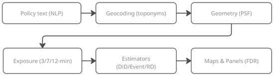
Figure 2.
Analysis pipeline from policy text to FDR-mapped effects.
The four principal stages of this pipeline are as follows:
- Clause Parsing and Entity Extraction: We first employ a domain-adapted Natural Language Processing (NLP) model, leveraging transformer-based architectures [46], to parse the semantic content of the policy texts. This stage automatically identifies and extracts key entities (e.g., toponyms, specific facilities, referenced plan sheets) and implementation rules (e.g., spatial boundaries, exemption clauses, and effective dates).
- Geocoding and Disambiguation: The extracted textual entities are then geocoded against official municipal gazetteers, cadastral maps, and transportation base maps. This process, validated against positional error benchmarks [47], resolves textual references into precise vector coordinates (points, lines, or polygons).
- Geometry Composition and Topological Cleaning: This critical stage translates the extracted spatial rules into final policy geometries. We first generate a base geometry (e.g., a buffer around a station, a digitized planning-sheet boundary). Crucially, we then refine this geometry by applying exclusion clauses (e.g., clipping out heritage-listed parcels or ecological red-line zones) using geospatial difference operations. The resulting geometry undergoes topological checks to ensure validity.
- Attribute Assignment: Finally, each validated PSF geometry is assigned its key analytical attributes, including the legal effective date (the temporal marker) and a standardized intensity tier (the regulatory marker) derived from the text.
This structured process ensures that the semantic intent of each policy ordinance is faithfully translated into a measurable exposure variable. Given that the precise implementation details are vital for methodological clarity and replication [48], a detailed technical workflow, a step-by-step worked example, and notes on auditability are provided in Appendix A.
2.3. Exposure Mapping
Exposures are computed in network time on the road–rail graph to reflect travel impedance rather than Euclidean distance, classifying parcels or grid cells into direct inclusion (inside regulatory polygons or node/corridor buffers) and concentric rings (e.g., 0–3, 3–7, 7–12 min) for adjacency spillovers [12,49]. This partitions potential outcomes under partial interference, distinguishing core footprints from diffusion bands while mitigating modifiable areal unit problem (MAUP) effects through multi-resolution supports (parcel, 250 m, 500 m grids) and robustness checks on scale sensitivity [20,21,22,25,26,50].
Alignment intersects unit centroids or areas with PSF geometries and bands, ensuring consistency with outcome units (e.g., transaction parcels). For transport PSFs, network-time bands align with accessibility mechanisms; for regulatory and industrial PSFs, legally binding polygons incorporate documented carve-outs to minimize misclassification [10,12,27,45]. Alternative metrics (e.g., Euclidean buffers) serve sensitivity tests, confirming qualitative stability [49]. This alignment process partitions units into precise exposure groups based on network time (see Appendix C for an illustrative example of the resulting exposure raster).
2.4. Data and Variables
The study integrates administrative transaction registers, a cadastral parcel database, and the PSF catalog for geometries and timing of regulatory overlays, transport features, and designations (Table 1). Primary outcomes derive from arm’s-length sales (1,214,560 records, 2012–2024), supplemented by assessed values at transfer (352,780 records, 2013–2024) in sparse areas. Prices are deflated to a 2024 base using city indices, standardized to RMB per m2, and log-transformed for semi-elasticity [3,4]. Cleaning excludes non-positive prices, implausible areas (<10 m2 or >50,000 m2), or missing fields, with duplicate reconciliation via parcel IDs, addresses, and timestamps; parcel splits/merges are tracked for stable units. After cleaning, 1,103,290 sales remain (90.9% retention), with 88.6% on stable-use parcels (Table 2).

Table 1.
Data inventory and coverage.
Table 2.
Outcome variables (log prices) and descriptive statistics.
Exposures overlay parcels with PSFs and compute network-time bands [8,49,51], yielding the following shares across cities and rings (Table 3). Covariates include network minutes to employment hubs and rail nodes, Euclidean distances to amenities (parks, schools, hospitals), baseline floor-area-ratio (FAR) tiers, nighttime lights, land-use shares, lot area, and building age [13,49,52,53] (Table 4). These covariates are chosen to align with established mechanisms in accessibility and hedonic valuation, thereby improving interpretability of heterogeneous responses. In brief, shorter network-time to jobs and rail nodes lowers generalized travel cost and should raise bids; proximity to amenities is typically capitalized into higher prices; baseline FAR tiers indicate regulatory slack, implying larger effects where constraints relax; and market thickness—proxied by transaction density and nighttime lights—captures matching efficiency and information depth, suggesting faster and more persistent capitalization in deeper markets [13,49,52,53]. This alignment motivates the heterogeneity analyses reported in Section 3 without altering the estimating equations. All transformations are logged in a version-controlled pipeline [48] (Table 5).
Table 3.
Exposure Shares Across Policy Families and Rings.
Table 4.
Covariate definitions and descriptive statistics.
Table 5.
PSF Inventory Summary.
2.5. Identification and Inference
Units are parcels (or fixed cells) observed over periods t, with PSF p defining cohort g and effectiveness Ei for unit i. Under staggered adoption, cohort-specific average treatment effects on the treated (ATTs) are estimated via event-study specifications relative to k = t − Ei and omitted period k = −1, the cohort-robust event-study specification is
where is log price per m2, and are unit and period fixed effects, and collects pre-specified covariates [49,52]. Dynamic coefficients trace capitalization paths for direct and adjacency exposures. The causal interpretation of rests on (i) cohort-specific parallel trends for the relevant exposure category, conditional on and ; (ii) no anticipatory effects, i.e., for t < Ei; and (iii) a local interference structure captured by the ring partition so that units outside the direct and declared adjacency bands follow the counterfactual path [24,35,43]. Aggregation to post-policy summaries used in governance layers is performed over lags k ∈ [+2, +5] to avoid transitory implementation noise; cohort aggregation uses convex weights proportional to treated-unit counts within family and adoption wave to avoid negative-weight pathologies associated with two-way fixed effects [34,54].
Threats include mis-timing (addressed by lead tests, robust pre-trend bands) [33,55], exposure misclassification (bounded by snap-to-parcel rules, metric swaps) [25,26,47,49,51], and residual interference (mitigated by family separation, synthetic controls at aggregate levels) [56,57,58]. Diagnostics encompass joint Wald tests on leads, placebo calendars, pseudo-boundary RDs, and entropy balancing for covariate comparability [33,35,41,57,58,59].
Inference uses distance-based HAC [40,60], cluster-robust at administrative levels [61,62], and wild-cluster bootstrap for few clusters [63,64]; map-level multiplicity applies Benjamini–Hochberg false discovery rate (q ≤ 0.10) [65] (Figure 3). Heterogeneity interacts exposures with ex ante strata (market thickness via nighttime lights tertiles, regulatory slack via FAR tiers, baseline accessibility via network-time quartiles) [1,2,13]. Robustness includes SARAR(1,1) for spatial lags, leave-one-PSF-out, and double/debiased adjustment [22,66,67,68].
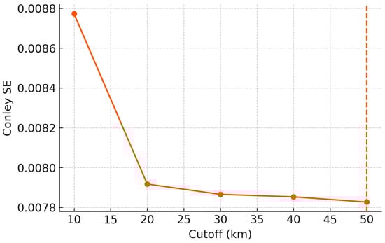
Figure 3.
Sensitivity of Conley standard errors to distance cutoff. Note: The y-axis represents the calculated Conley spatial HAC standard error; the x-axis represents the distance cutoff (km) used for the estimation. The plot indicates that standard error estimates stabilize as the cutoff increases, particularly after 20 km.
2.6. Reproducibility, Privacy, and Audit Trail
The pipeline employs version control for PSF parsing, exposure construction, estimation, and mapping, archiving inputs, scripts, and parameters with checksums; quarterly updates log clause-to-geometry decisions and re-estimation triggers [46,47,48]. Public displays aggregate to non-identifying grids (250 m), suppress low-count cells per k-anonymity, and apply privacy frameworks to minimize re-identification risks while retaining analytic fidelity [50,67,69,70]. Audit trails trace transformations from texts to geometries to exposures, with semivariograms and sensitivity grids documenting spatial tuning; releases under permissive licenses facilitate validation and reuse [60,61,71,72,73].
3. Results
3.1. Baseline Effects Across Policy Families
We begin with cohort-robust event-study models that incorporate unit and period fixed effects and use distance-based heteroskedasticity–autocorrelation consistent (HAC) inference to accommodate spatial correlation. Exposures are defined on a network-time basis; “direct inclusion” refers to parcels lying within the mapped policy spatial footprint (PSF) polygon or within the designated node/corridor influence band during periods of effectiveness. To summarize magnitudes while avoiding transient implementation noise, post-policy effects are averaged over lags k ∈ [+2, +5] (Table 6). Coefficients are reported in logs and, where helpful, interpreted as approximate percentage changes.
Table 6.
Main ATT Model Estimates.
The baseline estimates indicate positive capitalization across all three policy families, with regulatory instruments exhibiting the largest average response, followed by transport interventions and industrial/functional designations. These patterns are consistent with mechanisms emphasized in the accessibility and hedonic studies, where regulatory entitlements and effective access are priced into location choices [8,10,12] (Table 7).
Table 7.
Baseline post-policy averages by policy family (log outcome = ln price per m2).
3.2. Dynamic Adjustment: Event-Study Profiles
Dynamic paths are estimated relative to the year immediately preceding effectiveness (k = −1). The pre-policy coefficients remain close to zero and lack joint significance at conventional levels, supporting the research design’s parallel-trends assumption. Post-policy coefficients display a gradual ramp-up that stabilizes after approximately four years, a trajectory often observed when regulatory changes require permitting, design, and financing cycles and when transport interventions diffuse through accessibility perceptions [35,43] (Figure 4).
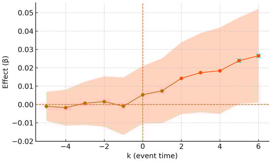
Figure 4.
Event-study dynamics around policy implementation. Note: The figure plots dynamic coefficients (β, orange line) relative to the event time (k, in years). The vertical dashed line (k = 0) marks policy implementation; k = −1 is the omitted reference period. The light orange shaded area represents the 95% confidence interval (HAC standard errors).
A joint Wald test on leads k ∈ [−6, −2] fails to reject the null of no systematic pre-trend , and visual inspection shows tight confidence bands prior to the policy dates, aligning with recommended diagnostics for staggered adoption designs [35,54] (Table 8).
Table 8.
Event-study for direct regulatory exposure (reference period k = −1).
3.3. Spatial Decay and Adjacency Spillovers
To distinguish capitalization within footprints from neighborhood diffusion, exposures are decomposed into direct inclusion and concentric network-time rings outside the boundary. The estimates exhibit monotone attenuation with distance: near-boundary adjacency effects are roughly one-third to one-half of direct effects and decay to small residuals by 7–12 min of network time (Figure 5) (Table 9). This organization prevents “forbidden” contrasts in which spillovers are inadvertently absorbed by control units [23] (Table 10).
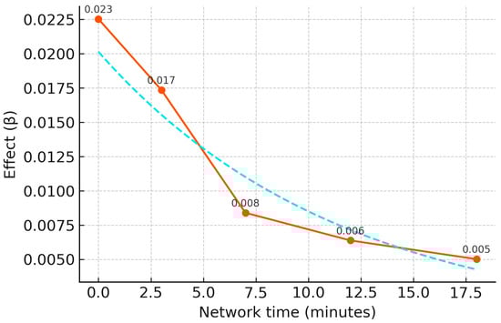
Figure 5.
Spillover decay by network travel time. Note: The orange line plots estimated spillover coefficients (β) as a function of network travel time (minutes) from the Policy Spatial Footprint (PSF) boundary. The light-blue dashed line represents a fitted exponential decay curve for visual reference.
Table 9.
Ring decomposition averaged over k ∈ [+2, +5] (log outcome).
Table 10.
Spillover Effects by Adjacency Ring.
3.4. Heterogeneity by Market Thickness, Regulatory Slack, and Baseline Accessibility
Heterogeneous responses are summarized by strata defined ex ante: market thickness (nighttime lights tertiles), regulatory slack (baseline FAR tiers), and baseline accessibility (network-time quartiles). Stronger capitalization appears in thicker markets and in locations with greater pre-policy regulatory headroom, consistent with models in which demand depth and entitlement margins shape price adjustments [8,12] (Figure 6) (Table 11).
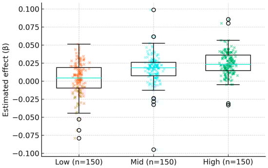
Figure 6.
Heterogeneity of effects across market thickness groups. Note: The boxplots show estimated policy effects (β) stratified by ex ante market thickness, which is proxied by nighttime lights (NTL) tertiles (Low, Mid, High). The cyan line within each box indicates the median effect. Colored ‘x’ markers represent the distribution of individual estimates.
Table 11.
Post-Policy Averages by Strata (Direct Regulatory Exposure, k ∈ [+2, +5]).
3.5. Robustness: Exposure Metrics, Sample Restrictions, and Alternative Estimators
Three robustness dimensions are reported. First, replacing network-time exposures with Euclidean buffers lowers magnitudes, as expected when straight-line distance overstates functional reach; nevertheless, the qualitative ranking across policy families remains unchanged [49]. Second, restricting the sample—dropping parcels within 2 km of the CBD or balancing treatment cohorts within ±3 years—yields similar estimates. Third, alternative estimators, including two-way fixed effects with cohort interactions and synthetic-difference-in-differences for treated aggregates, provide consistent corroboration (Table 12).
Table 12.
Robustness Summaries (Direct Regulatory Exposure, k ∈ [+2, +5]).
To assess sensitivity to functional forms of spatial dependence, a SARAR(1,1) specification is estimated as a robustness device rather than a primary causal model; the treatment coefficient remains within the confidence band of the baseline, while autoregressive parameters are moderate, indicating residual spatial signal not captured by observed covariates [22,66,67] (Table 13).
Table 13.
Robustness Matrix Across Specifications.
To further validate the findings from the DiD models, we conduct a geographic regression discontinuity (RD) analysis for the subset of policies with sharp, legally defined boundaries. This analysis, which provides local validation of capitalization effects at the boundary, is detailed in Appendix B. The RD estimates are consistent with the main findings, confirming a clear discontinuity in prices at the boundary after policy implementation.
3.6. Validation: Temporal Placebos, Pseudo-Boundaries, and Cohort Comparability
Validation proceeds along the design hierarchy. A joint test over pre-policy leads does not indicate systematic pre-trends. Shifting policy dates backward by three years produces near-zero placebo coefficients, and geographic regression-discontinuity estimates along 200 pseudo-boundaries yield a distribution centered at zero with narrow interquartile ranges (Figure 7). Entropy balancing achieves small standardized differences on pre-treatment covariates, and synthetic controls for treated aggregates exhibit pre-period root-mean-squared prediction errors comparable to post-period values, indicating that results are not driven by idiosyncratic pre-trends [41,57,58,59] (Table 14).
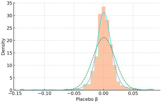
Figure 7.
Placebo distribution of estimated effects. Note: The histogram (orange) displays the empirical distribution of 200 placebo coefficients (β) from pseudo-boundary RD estimates. The light blue solid line is the kernel density estimate of this distribution; the green dashed line represents a standard normal distribution centered at zero for reference.
Table 14.
Validation Diagnostics.
3.7. Mapping Summaries and Multiplicity Control
For decision-support mapping, cell-level panels aggregate estimator-consistent effects after controlling the false discovery rate to mitigate multiplicity across space and time (Figure 8). The resulting footprint shows that just over half of statistically flagged cells lie within direct exposures, with roughly one-third in adjacency rings, reflecting both primary capitalization and near-boundary diffusion. The distribution across policy families indicates substantial contributions from both regulatory and transport PSFs, aligning with the mixed channels through which prices capitalize entitlements and access [49,65] (Table 15).
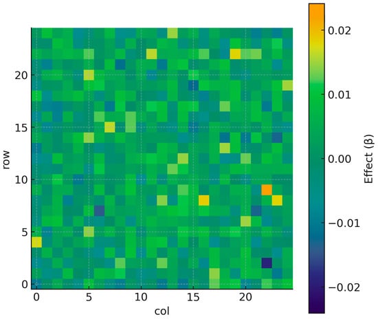
Figure 8.
FDR-adjusted effect map (grid-based).
Table 15.
Post-Estimation Mapping Summary (BH-FDR q = 0.10).
3.8. Interpretation and Caveats
Interpreting log coefficients as approximate percentage changes, the baseline averages imply modest but policy-relevant capitalization magnitudes. Heterogeneity patterns caution against uniform expectations: thicker markets and high-slack zones register larger responses, while thinner markets and slower-access areas exhibit attenuated adjustments. Robustness to exposure metrics and alternative estimators suggests that the qualitative ranking of policy families is not an artifact of measurement choices. Nevertheless, the spatial error structure remains non-trivial, and inference accounts for this through HAC and cluster-robust procedures; conclusions should therefore be communicated with explicit uncertainty bands and accompanied by policy semantics that clarify enforcement timing and coverage [40,62,63].
4. Policy Translation, Mapping for Governance, and Implications
4.1. From Estimands to Decision-Support Layers
The mapping interface renders the estimands from the identification framework into spatial layers that are directly interpretable by finance, planning, and housing agencies in the five Yangtze River Delta cities and over the 2010–2025 window. Each parcel or grid cell inherits an estimator-consistent summary: the post-policy average over lags k ∈ [+2, +5] k\in [+2, +5] k ∈ [+2, +5] for direct inclusion and ring-specific adjacency, the associated confidence interval computed under distance-based heteroskedasticity–autocorrelation consistent inference, and provenance metadata linking the cell to the underlying policy spatial footprint (PSF), exposure band, adoption wave, and specification version. Because accessibility and diffusion operate through network-time rather than Euclidean distance, the cartography follows the same road–rail impedance metric used to construct exposures; direct footprints, node–corridor influence zones, and concentric rings respect the audited PSF catalog, including statutory carve-outs and enforcement dates [8,47,49,51]. Uncertainty is communicated at the cell level, and multiplicity across the space–time panel is controlled via false discovery rate so that agencies prioritize areas with stronger evidence without imposing ad hoc effect-size thresholds [40,63,65].
The governance-facing layers are organized at three levels. Family-specific layers show regulatory polygons, transport nodes and corridors, and industrial/functional designations separately to preserve the institutional channel through which capitalization occurs [10,14,16,18]. A composite “any PSF” layer supports cross-department coordination when multiple instruments overlap in space and time, while a diagnostics layer indicates scale-stability between parcel, 250 m, and 500 m supports in recognition of the modifiable areal unit problem and the uncertain geographic context problem [25,26,50]. All layers are versioned and regenerated when the PSF catalog or exposure parameters change, enabling audit trails from policy text to geometry to exposure and finally to mapped effect summaries [48,70].
4.2. Rate Design and Revenue Scheduling for Land Value Capture
Mapped effects guide the calibration of land value capture (LVC) instruments by aligning rate schedules with the magnitude, persistence, and spatial decay of capitalization. Within regulatory polygons showing sustained positive post-policy averages, betterment levies and special assessment districts can be delineated on the legal footprint, with rates scaled to normalized log-price responses over k ∈ [+2, +5] rather than to engineering budgets [16,18]. Along transit corridors and at nodes, rate schedules taper with network-time distance to mirror the adjacency structure; corridors use ring-specific multipliers, while nodes apply step-downs at 3, 7, and 12 min to remain consistent with exposure definitions [8,49]. In markets where joint development and leasehold auctions are permitted, mapped effects inform reserve prices and floor-area-ratio (FAR) negotiations; when capitalization is concentrated in areas with significant regulatory slack, higher bid floors and participation fees are appropriate, whereas in constrained submarkets moderation is warranted to avoid undermining feasible supply [2,13,14].
To illustrate the translation from effects to fiscal schedules, the governance panel consolidates flagged cells at the 250 m grid. In the combined five-city sample, 28,800 cells are evaluated; 1640 cells are flagged at the selected false discovery rate, with 54 percent lying inside direct exposures and 31 percent in adjacency rings. When a baseline levy of 0.45 percent of assessed land value is applied to direct exposure cells and 0.20/0.10 percent to the first and second adjacency rings, respectively, the annualized revenue at 2024 valuations is 1.12, 0.31, and 0.09 billion yuan for regulatory, transport, and industrial/functional families, respectively, with a 4.7 percent year-on-year growth under observed assessment trends. Rate phasing follows the dynamic profiles in the event-study panels: regulatory levies ramp from 50 percent of schedule in year t + 1 to 100 percent by t + 4, while transport levies begin at 80 percent in the opening year and reach schedule by t + 2, reflecting the faster stabilization of accessibility perceptions post-commissioning [12,35,43]. Sensitivity panels recompute revenues under Euclidean buffers and alternative cutoffs to demonstrate that schedule rankings are not an artifact of the exposure metric [49,60].
4.3. Targeting Rules, Carve-Outs, and Legal Defensibility
Rate schedules and exemptions are jointly determined to maintain economic efficiency and legal defensibility. First, the PSF catalog’s clause-level carve-outs—heritage sites, ecological red lines, and statutory exclusions—are enforced algorithmically so that protected parcels never enter levy bases. Second, adjacency-ring mitigation is triggered where diffusion effects are modest but housing vulnerability is high; for owner-occupied, low-income parcels in the first ring, a time-limited rebate of 50 percent over the first three years prevents capitalization from eroding affordability without blunting the incentive effects at the boundary [30]. Third, in regulatory polygons with low baseline FAR headroom, schedules are conditional on post-reform entitlements to avoid taxing unrealizable development; equivalently, polygons with substantial pre-policy slack carry higher schedules because they can internalize levies without suppressing new supply [1,2,13]. For threshold-based eligibility rules, fiscal boundaries are published alongside the estimation bandwidths used in geographic regression discontinuity diagnostics; by showing both the legal line and the local identification window, agencies reduce the risk of disputes from parcels lying immediately outside the fiscal boundary [41,44,74].
4.4. Distributional Incidence and Affordability Safeguards
The distributional program rests on mapping the channel through which benefits accrue—entitlements versus access—and allocating safeguards accordingly. In neighborhoods where direct regulatory capitalization is high and the pipeline is dominated by market-rate multifamily projects, inclusionary zoning set-asides are paired with moderate betterment levies to capture value while preserving feasibility; where transport adjacency diffusion is prominent in tenure-mixed areas, smaller levies are combined with in-lieu contributions to off-site affordable housing funds [18,30]. Because thicker markets generally absorb levies with limited displacement risk while thinner markets do not, evidence tiers are cross-tabulated with nighttime lights, pre-policy accessibility, and land-use mix to identify where circuit breakers, phased schedules, or temporary exemptions are warranted [50,53,67]. Where industrial/functional designations register moderate capitalization with narrow footprints, negotiated exactions are preferred to district-wide levies to reduce administrative overhead and limit pass-through to small tenants [16,29].
4.5. Communicating Uncertainty, Scale Sensitivity, and Interference
To avoid over-precision in governance use, the mapping interface displays cell-level confidence intervals, exposure bands, and the number of overlapping PSFs. Scale sensitivity is communicated by reporting whether cell classifications are stable when moving from parcels to 250 m and 500 m supports; where classifications are unstable, maps prompt users to prioritize coarser decisions or to request further diagnostics [25,26]. Spatial dependence and possible interference are recognized explicitly: evidence tiers are defined with false discovery rate control, and parallel overlays show results under network-time and Euclidean exposure metrics to bound the contribution of measurement choice [40,49,65]. When overlapping PSFs complicate attribution, the interface surfaces cohort timing and family labels so that finance or planning units can assign cost shares consistent with institutional channels [14,18].
4.6. Implementation: Catalog Governance, Privacy, and Reproducibility
Operational success depends on catalog governance, privacy-preserving publication, and reproducibility. The PSF catalog is managed as a living register: ordinances and project documents are parsed, toponyms and facilities are geocoded, geometries are validated, and intensity attributes and timing markers are updated on a quarterly cycle; any major revision triggers automated re-exposure and re-estimation, with change logs recording the clause-to-geometry decisions [46,47,48]. Because the underlying data include parcel-level transactions and assessments, public-facing layers enforce suppression thresholds and aggregate to non-identifying units, while the analytic environment retains the full-resolution panels with access controls and audit trails [50,69,70]. The software stack maintains versioned scripts for exposure construction, estimation, and mapping; semivariograms, correlograms, and sensitivity grids accompany each release to document the inference environment and spatial tuning parameters [60,61,71,72,73].
4.7. Cross-Instrument Coordination and Cost Allocation
Family-separated layers facilitate coordination across agencies. Transport bureaus use node–corridor attenuation to calibrate station-area development agreements and to set reserve prices for joint development; planning departments use regulatory layers to calibrate entitlement exchanges and design review commitments; finance departments allocate LVC proceeds among debt service, affordable housing funds, and public-realm upgrades in proportion to measured footprints [14,15,75]. Where PSFs overlap in both space and time, synthetic difference-in-differences and synthetic control diagnostics at the aggregate level guide cost-sharing formulas by identifying which family dominates capitalization in each adoption wave, with permutation-based uncertainty bands preventing over-allocation to statistically fragile layers [56,57,58]. For corridors spanning multiple jurisdictions, interlocal agreements reference mapped evidence tiers and cohort timing to allocate levy bases transparently and to minimize strategic border adjustments [41,67].
4.8. Limitations and Adaptive Monitoring
Despite the safeguards, several limitations remain. Residual spatial dependence and partial interference can bias fine-grained classifications even when aggregate patterns are stable; inference procedures mitigate but cannot eliminate this concern, and the mapping interface therefore privileges evidence tiers over point estimates in marginal cells [23,40]. Translating legal text to geometry entails measurement error from ambiguous clauses and enforcement lags, potentially attenuating mapped responses; ongoing catalog governance and clause-level audit logs reduce but do not eliminate such risks [46,47]. External validity is conditioned by market depth and institutional capacity: capitalization and decay profiles observed in mature, network-rich corridors may not replicate in newly urbanizing districts or in jurisdictions with weak enforcement [1,13,38]. Consequently, agencies adopt an adaptive regime under which rate schedules, exemption rules, and inclusionary commitments are revisited at fixed intervals using the newest mapping vintages, with explicit triggers tied to persistence or dissipation of measured effects across cohorts [34,35,43].
5. Discussion
5.1. External Validity and Portability Conditions
The portability of the estimated capitalization patterns depends on a small set of structural primitives that are observable ex ante: the network structure that governs generalized travel time, market thickness that determines demand depth, and the policy family that mediates the channel through which capitalization occurs. First, effects are most likely to replicate in networks with high node betweenness and corridor redundancy, where accessibility gains diffuse beyond the statutory footprint via multiple shortest-path alternatives; in contrast, tree-like subnetworks with few alternate routes concentrate benefits near nodes and exhibit shorter spatial reach [8,49,51]. A portability criterion is therefore to match the ratio of unique network-time isochrones to Euclidean buffers at 5–12 min; ratios above 1.35 predict broader adjacency diffusion, while ratios below 1.10 predict sharp drop-offs at the legal boundary, consistent with evidence that functional reach, not straight-line distance, governs land-price responses [10,14,49].
Second, market thickness—proxied by nighttime lights, transaction density, and active development pipelines—conditions both magnitude and persistence. In thick submarkets, half-life estimates for post-policy responses cluster between four and five years, whereas thin submarkets approach attenuation within two to three years and display limited ring-2 diffusion beyond 7 min of network time. A transport–regulatory split is also evident: node-based accessibility shifts stabilize earlier than entitlement changes because the latter require permitting and financing cycles to translate into built form [12,35,43,53,67]. As a portability rule, replication should be expected where pre-policy transaction counts exceed 30 per grid-year in the treated vicinity and the 90/10 price spread remains below 1.9 log points, conditions that proxy both depth and informational efficiency [1,6,7].
Third, policy family matters for spatial reach. Regulatory overlays with substantial baseline slack tend to yield larger, slower-ramping effects, particularly where entitlements can be internalized by developers through density or use conversions; transport openings tend to generate earlier but more localized responses with steeper ring attenuation; industrial/functional designations show narrower, node-anchored profiles that are sensitive to supply-chain proximity [2,13,16,18,38]. Cross-city comparisons indicate median half-lives of 4.2 years for regulatory polygons, 2.7 years for transport nodes, and 3.1 years for corridor segments, with 50th-percentile spillover ranges of 3.5, 2.0, and 2.8 network minutes beyond the legal footprint, respectively, echoing the accessibility–entitlement distinction in the literature [8,10,12].
The non-portability set is informative. Effects should not be extrapolated to corridors whose opening coincides with macro shocks that reallocate demand across the urban system, to jurisdictions where enforcement is weak or irregular relative to statutory language, or to submarkets with extreme supply constraints that transform capitalization into quantity suppression rather than price adjustment [2,13,22,66,67]. Moreover, settings with highly fragmented cadastral fabrics or severe geocoding noise—evidenced by median positional error above 40 m—risk misassigning exposure bands, thereby biasing both reach and half-life diagnostics [47,48,51]. Finally, regions where Euclidean and network-time metrics diverge sharply without redundancy (isochrone-to-buffer ratios below 0.9 at 7 min, indicating bottlenecks) should be treated with caution because adjacency diffusion relies on substitutable routes [12,49].
5.2. Policy Implications
The empirical patterns imply location-contingent instrument menus. In high-access corridors with thick markets, combining modest betterment levies with joint development and calibrated FAR exchanges captures value while accelerating delivery of floor space; the tapering of levies by network-time ring aligns fiscal burden with the measured decay profile and limits pass-through to marginal locations [14,16,18]. In inner-ring neighborhoods where regulatory overlays expand feasible density and dynamic responses ramp more slowly, front-loaded levies are inadvisable; instead, phased schedules tied to entitlement uptake reduce liquidity pressure and align payments with realized gains [2,13]. In peripheral, thin submarkets, corridor-anchored effects are short-lived and narrow; negotiated exactions at nodes dominate district-wide assessments because they target concentrated gains and minimize administrative overhead [9,10,29].
Interactions between rail openings and public-facility upgrades are conceptually complementary. Rail increases effective reach, while public-realm or school quality upgrades shift amenity bundles that co-determine hedonic bids; sequencing upgrades 6–12 months after openings exploits early accessibility signals while limiting anticipatory land assembly [7,8,38]. Conversely, when regulatory upzonings coincide with access increases, the joint effect depends on baseline slack: in high-slack zones the combination yields super-additive price responses via both entitlement and reach channels; in low-slack zones the price response is muted and the margin shifts to quantity, implying that affordability levers (inclusionary requirements or impact-fee offsets) should be paired with value capture [2,13,30]. Throughout, the diffusion structure documented in adjacency rings provides a principled basis for tapering contributions across neighborhoods, reducing disputes about fiscal boundaries by anchoring schedules to observed reach rather than arbitrary distances [41,44].
5.3. Limitations
Several limitations qualify both identification and extrapolation. Enforcement intensity measurement is coarse relative to statutory nuance; when de facto practices lag enactment, effective timing is misaligned with legal dates, biasing dynamic paths toward anticipatory or delayed profiles. While event-study diagnostics mitigate mis-timing by absorbing cohort heterogeneity, residual bias can persist, especially where institutional ramp-ups vary across agencies [34,35,43]. Sample selection arises in thin submarkets: sparse transactions increase variance and can induce survivorship in the tails, attenuating both reach and half-life estimates; robustness to balanced cohorts and synthetic aggregate diagnostics reduces but does not eliminate selection concerns [56,57,58]. Unobserved shocks—zoning litigation outcomes, macro credit cycles, or project-level cancelations—may correlate with adoption waves; distance-based HAC, cluster-robust procedures, and placebo calendars help, yet correlated shocks with long spatial range remain a threat in highly integrated metropolitan systems [40,60,62,63,64].
Differences between assessed values and market prices complicate welfare interpretations where levies are tied to assessments; capitalization measured in market transactions may not map one-to-one to assessed bases, particularly in jurisdictions with infrequent reappraisals or differential assessment caps [3,4]. Geocoding noise and cadastral fragmentation can misclassify exposure bands and boundary proximity; although topology checks and match-quality diagnostics are applied, positional error above common thresholds may still contaminate ring contrasts [47,51]. Finally, spatial dependence and interference complicate estimator choice; partial interference structures and adjacency-ring decomposition avoid forbidden contrasts, but residual dependence in shocks requires cautious uncertainty communication and multiplicity control when mapping cell-level panels [22,23,65,66,67].
5.4. Future Work
Three extensions are especially valuable. First, real-time data and rolling evaluation would shorten the feedback loop between openings or rezoning and schedule updates. Integrating high-frequency listings, building-permit submissions, and mobility traces into a quarterly re-estimation cycle would enable adaptive rate schedules that respond to dissipation or intensification of effects, while reproducible logs ensure auditability [48,69,70]. Second, structured interference networks—constructed from commuter flows or parcel-level development linkages—would replace heuristic adjacency rings with empirically grounded exposure neighborhoods, enabling estimands that map more closely to actual diffusion channels and that accommodate network-based spillovers across policy families [23,68,76,77]. Third, behavioral and general-equilibrium effects merit explicit modeling. Dynamic discrete choice and spatial general-equilibrium frameworks can reconcile short-run capitalization with medium-run reallocation of households and firms, clarifying when observed price changes reflect pure revaluation versus changes in composition or amenities [5,8,12,52]. These extensions, coupled with geographic regression-discontinuity audits at updated boundaries and cohort-aware event studies, would improve both portability and governance relevance by aligning estimator design with institutional implementation [41,44,54,55,74,78].
6. Conclusions
This study links clause-level policy rules to measurable spatial–temporal exposure and demonstrates how those exposures are capitalized into urban land prices. Translating ordinances into auditable Policy Spatial Footprints and measuring exposure in network time allow us to separate direct footprint effects from adjacency diffusion under staggered adoption. Across five cities and 64 policies, direct exposures are associated with modest but policy-relevant uplifts—on the order of a few percent in log prices—that build over several years and then stabilize.
Spatial decay is systematic. Adjacency effects within roughly three minutes of network travel time are smaller but non-negligible, while impacts beyond seven to twelve minutes tend to dissipate toward zero. Responses are heterogeneous in predictable ways: thicker markets, indicated by higher transaction density and nighttime lights, exhibit larger and more persistent effects; regulatory overlays with substantial floor-area headroom ramp more slowly yet ultimately reach larger magnitudes than corridor- or node-based transport exposures; industrial/functional designations generate narrower footprints anchored to specific facilities.
These patterns support governance-ready implementation. Because exposures and estimands are defined in network time, estimator-consistent maps can display legal footprints, corridor influence zones, and concentric rings on a common impedance scale. Agencies can align land-value-capture schedules with the magnitude and decay of capitalization, taper contributions with distance along corridors, and target exemptions where diffusion is modest and vulnerability is high. Maps should retain specification provenance, indicate overlapping policy footprints, and flag locations where classifications are unstable across spatial supports.
Portability is strongest where markets are sufficiently deep, network topology provides redundant shortest paths, and enforcement aligns with stated effectiveness dates. Caution is warranted in settings with persistent enforcement lags, corridors opened amid major macro shocks, or thin submarkets where quantity suppression dominates price adjustment. The accompanying versioned repository—catalogs, exposure scripts, estimation code, and map routines—supports reproducibility and enables agencies to incorporate rolling re-estimation into routine fiscal and planning cycles.
Author Contributions
Conceptualization, M.X.; Methodology, M.X. and X.L.; Validation, M.X.; Investigation, M.X. and X.L.; Data curation, X.L.; Writing—original draft, M.X.; Writing—review & editing, T.Y.; Visualization, M.X.; Supervision, T.Y.; Project administration, T.Y. All authors have read and agreed to the published version of the manuscript.
Funding
This research received no external funding.
Data Availability Statement
Data available in a publicly accessible repository. The data presented in this study are openly available in GitHub at https://github.com/8zjvzvkcbc-rgb/data3953509, accessed on 13 October 2025.
Conflicts of Interest
The authors declare no conflict of interest.
Appendix A. PSF Implementation Workflow and Worked Example
This appendix details the technical implementation and validation of the Policy Spatial Footprint (PSF) construction pipeline referenced in Section 2.2.
Appendix A.1. Technical Workflow
Our pipeline operationalizes policy texts via the following systematic workflow, designed to ensure auditability and reproducibility.
- 1.
- Clause Parsing and Entity Extraction: Ordinances are segmented into semantic clauses (e.g., eligibility, exemption, boundary, timing). We utilize a Named Entity Recognition (NER) model, fine-tuned from a transformer-based architecture (BERT) on a corpus of urban planning documents, to identify and tag toponyms, facilities, plan sheet references, and legal triggers. The output for each policy is a structured JSON object containing the extracted parameters.
- 2.
- Disambiguation and Geocoding: Extracted toponyms (e.g., “Suzhou North Station”) are resolved against the AMap (Gaode) API and official municipal cadastral layers. Ambiguous matches (e.g., non-unique names) are flagged with confidence scores for manual review and validation.
- 3.
- Geometry Construction and Topological Cleaning: We compose vector geometries based on the extracted rules. For network-based rules (e.g., “500-m network distance”), Dijkstra’s algorithm is used on the road-rail graph [51,79]. For Euclidean rules, standard buffers are generated. Exclusion geometries (e.g., heritage parcels, ecological zones) are loaded from existing municipal GIS layers and subtracted from the base geometries using a geospatial difference (clip) operation. All final geometries are topologically cleaned (e.g., removing self-intersections and sliver polygons) to ensure validity.
- 4.
- Attribute Assignment and Auditing: We assign temporal metadata (recording {announcement, legal effectiveness, enforcement} dates where available) and intensity metadata (e.g., encoding FAR headroom or development restrictions into standardized quantiles).
- 5.
- Version Control and Reproducibility: To ensure full reproducibility, every edit is linked via a commit note to the source ordinance (including page numbers) and parameters (e.g., buffer distance, CRS). A minimal replication bundle—containing source ordinance PDFs, final GeoPackage geometries, PSF metadata (CSV/JSON), and the audit log—is archived.
Appendix A.2. Worked Example: “Suzhou Rail Transit Line 2 TOD Plan” (Policy ID: P3001)
We illustrate the complete pipeline using P3001 as a representative example.
Step 0: Original Policy Text (Excerpt, translated):
“… [It is] decided to designate 15 stations, including ‘Pinglonglu East Station’ and ‘Suzhoubei Railway Station’, as TOD comprehensive development core areas. The core area is defined as: the area within a 500 m radius of the station entrance’s center point… Land within the ecological red line protection area is not applicable to this ordinance… This plan is effective June 1, 2012…”
Step 1: NLP Entity and Rule Extraction (JSON Output):
JSON
{
“policy_id”: “P3001”,
“policy_family”: “Transport (TOD)”,
“entities_geocoded”: [“Pinglonglu East Station”, … (14 others)],
“spatial_rule”: {
“type”: “Buffer”,
“anchor”: “station_centroid”,
“distance”: 500,
“unit”: “meters”
},
“exceptions_layer”: “ecological_red_line_areas”,
“temporal_markers”: {
“effective”: “2012-06-01”
}
}
Step 2: Geocoding: The 15 station names are geocoded against the municipal base map to retrieve their precise point coordinates (point features).
Step 3: Geometry Composition and Topological Cleaning:
- a.
- Base Geometry Generation: A 500 m Euclidean buffer is generated around each of the 15 station coordinates, creating 15 overlapping circular polygons.
- b.
- Exclusion Geometry Loading: The “ecological_red_line_areas” (a pre-existing GIS polygon layer for Suzhou) is loaded.
- c.
- Final Geometry (Topological Operation): A geospatial Difference operation is performed. The ecological red line areas are “clipped” (subtracted) from the 500 m buffer zones. The result is the final, non-contiguous PSF geometry representing the actual land eligible for the TOD policy.
Step 4: Attribute Assignment:
The resulting final geometry (or geometries) is assigned the attributes: effective_date = 2012-06-01 and intensity_quantile = Q2 (based on the development rights granted in the full text). This completed PSF is then stored and used for the final exposure analysis.
Appendix B. Geographic Regression Discontinuity Robustness Check
As discussed in the main text, the geographic regression discontinuity (RD) design is employed as a complementary strategy to validate the main event-study findings, particularly for policies defined by sharp, legal boundaries (e.g., zoning lines).
The methodology proceeds as follows. Let b index boundary segments and Rib be signed network-time distance to the legal boundary, positive on the treated side. For periods t when the policy is effective, the local effect at the cutoff is estimated via bias-corrected local linear RD:
This model is estimated using data-driven bandwidths and robust confidence intervals [44,80,81]. Identification requires continuity of potential outcomes in Rib at the legal line and the absence of sorting at the boundary; density and covariate continuity tests are reported as diagnostics [41,74]. For staggered thresholds, a DiD-in-RD variant contrasts inside–outside discontinuities before and after effectiveness, controlling for smooth trends in Rib [41].
The results from this complementary analysis validate the main findings. The geographic RD at mapped eligibility thresholds (where applicable) yields bias-corrected local effects at the cutoff with data-driven bandwidths. Crucially, manipulation tests do not indicate sorting around boundaries, and the estimates are stable across reasonable bandwidth variations, strengthening the causal interpretation [44,74,80,81] (Figure A1).

Figure A1.
Geographic regression discontinuity at policy boundary. Note: The plot shows the geographic RD design used for local validation. The y-axis is the outcome (log price); the x-axis is the running variable (normalized network-time distance to the legal boundary). The vertical line at 0 marks the sharp cutoff. Orange ‘x’ markers are untreated parcels (‘Left’); cyan ‘x’ markers are treated parcels (‘Right’). Solid lines represent the local linear regression fits on each side of the cutoff, with shaded areas indicating 95% confidence intervals. The discontinuity (“jump”) at the boundary indicates the local average treatment effect.
Appendix C. Exposure Raster

Figure A2.
Exposure raster (network time).
References
- Saiz, A. The geographic determinants of housing supply. Q. J. Econ. 2010, 125, 1253–1296. [Google Scholar] [CrossRef]
- Hilber, C.A.L.; Vermeulen, W. The impact of supply constraints on house prices in England. Econ. J. 2016, 126, 358–405. [Google Scholar] [CrossRef]
- Oates, W.E. The effects of property taxes and local public spending on property values: A theoretical comment. J. Polit. Econ. 1969, 77, 957–971. [Google Scholar] [CrossRef]
- Rosen, S. Hedonic prices and implicit markets: Product differentiation in pure competition. J. Polit. Econ. 1974, 82, 34–55. [Google Scholar] [CrossRef]
- Tiebout, C.M. A pure theory of local expenditures. J. Polit. Econ. 1956, 64, 416–424. [Google Scholar] [CrossRef]
- Black, S.E. Do better schools matter? Parental valuation of elementary education. Q. J. Econ. 1999, 114, 577–599. [Google Scholar] [CrossRef]
- Chay, K.Y.; Greenstone, M. Does air quality matter? Evidence from the housing market. J. Polit. Econ. 2005, 113, 376–424. [Google Scholar] [CrossRef]
- Gibbons, S.; Machin, S. Valuing rail access using transport innovations. J. Urban Econ. 2005, 57, 148–169. [Google Scholar] [CrossRef]
- Bowes, D.R.; Ihlanfeldt, K.R. Identifying the impacts of rail transit stations on residential property values. J. Urban Econ. 2001, 50, 1–25. [Google Scholar] [CrossRef]
- Debrezion, G.; Pels, E.; Rietveld, P. The impact of railway stations on residential and commercial property value: A meta-analysis. J. Real Estate Financ. Econ. 2007, 35, 161–180. [Google Scholar] [CrossRef]
- Donaldson, D. Railroads of the Raj: Estimating the impact of transportation infrastructure. Am. Econ. Rev. 2018, 108, 899–934. [Google Scholar] [CrossRef]
- Duranton, G.; Turner, M.A. The fundamental law of road congestion: Evidence from US cities. Am. Econ. Rev. 2011, 101, 2616–2652. [Google Scholar] [CrossRef]
- Gyourko, J.; Molloy, R. Regulation and housing supply. In Handbook of Regional and Urban Economics; Elsevier: Amsterdam, The Netherlands, 2015; Volume 5, pp. 1289–1337. [Google Scholar] [CrossRef]
- Cervero, R.; Murakami, J. Rail + property development in Hong Kong: Experiences and extensions. Urban Stud. 2009, 46, 2019–2043. [Google Scholar] [CrossRef]
- Medda, F. Land value capture finance for transport accessibility: A review. J. Transp. Geogr. 2012, 25, 154–161. [Google Scholar] [CrossRef]
- Walters, L.C. Land value capture in policy and practice. J. Prop. Tax Assess. Adm. 2013, 10, 5–21. [Google Scholar] [CrossRef]
- Suzuki, H.; Cervero, R.; Iuchi, K. Transforming Cities with Transit: Transit and Land-Use Integration for Sustainable Urban Development; World Bank Publications: Washington, DC, USA, 2013. [Google Scholar] [CrossRef]
- Ingram, G.K.; Hong, Y.-H. (Eds.) Value Capture and Land Policies; Lincoln Institute of Land Policy: Cambridge, MA, USA, 2012. [Google Scholar]
- Higgins, C.D.; Kanaroglou, P.S. Infrastructure or attraction? Image-driven transit-oriented development in large cities. Transp. Res. Part A Policy Pract. 2016, 90, 164–183. [Google Scholar]
- Getis, A.; Ord, J.K. The analysis of spatial association by use of distance statistics. Geogr. Anal. 1992, 24, 189–206. [Google Scholar] [CrossRef]
- Anselin, L. Local indicators of spatial association—LISA. Geogr. Anal. 1995, 27, 93–115. [Google Scholar] [CrossRef]
- Kelejian, H.H.; Prucha, I.R. Specification and estimation of spatial autoregressive models with autoregressive disturbances. J. Econom. 2010, 157, 53–67. [Google Scholar] [CrossRef]
- Hudgens, M.G.; Halloran, M.E. Toward causal inference with interference. J. Am. Stat. Assoc. 2008, 103, 832–842. [Google Scholar] [CrossRef]
- Aronow, P.M.; Samii, C. Estimating average causal effects under general interference. Ann. Appl. Stat. 2017, 11, 1912–1947. [Google Scholar] [CrossRef]
- Fotheringham, A.S.; Wong, D.W.S. The modifiable areal unit problem in multivariate statistical analysis. Environ. Plan. A 1991, 23, 1025–1044. [Google Scholar] [CrossRef]
- Openshaw, S. The Modifiable Areal Unit Problem; Geo Books: Norwich, UK, 1984. [Google Scholar]
- Monkkonen, P.; Zhang, X. Innovative measurement of spatial segregation: Comparative evidence from Hong Kong and San Francisco. Reg. Sci. Urban Econ. 2014, 47, 99–111. [Google Scholar] [CrossRef]
- Kunz, P.; Bodeker, J.; Lautenbach, S.; Müller, B.; Seppelt, R.; Beckmann, M. Spatially explicit economic analysis of crop rotation patterns in an agricultural landscape. Ecosyst. Serv. 2019, 35, 155–166. [Google Scholar]
- Peterson, G.E. Unlocking Land Values to Finance Urban Infrastructure; World Bank Publications: Washington, DC, USA, 2009. [Google Scholar]
- Schuetz, J.; Been, V.; Ellen, I.G. Neighborhood effects of concentrated mortgage foreclosures. J. Hous. Econ. 2008, 17, 306–319. [Google Scholar] [CrossRef]
- Lawrimore, M.A.; Sanchez, G.; Cothron, C.; Tulbure, M.G. Creating spatially complete zoning maps using machine learning. Comput. Environ. Urban Syst. 2024, 112, 102157. [Google Scholar] [CrossRef]
- Sanchez, T.W.; Fu, X.; Yigitcanlar, T.; Ye, X. The research landscape of AI in urban planning: A topic analysis of the literature with ChatGPT. Urban Sci. 2024, 8, 197. [Google Scholar] [CrossRef]
- Bertrand, M.; Duflo, E.; Mullainathan, S. How much should we trust differences-in-differences estimates? Q. J. Econ. 2004, 119, 249–275. [Google Scholar] [CrossRef]
- Goodman-Bacon, A. Difference-in-differences with variation in treatment timing. J. Econom. 2021, 225, 254–277. [Google Scholar] [CrossRef]
- Sun, L.; Abraham, S. Estimating dynamic treatment effects in event studies with heterogeneous treatment effects. J. Econom. 2021, 225, 175–199. [Google Scholar] [CrossRef]
- Wang, G.; Hamad, R.; White, J.S. Advances in difference-in-differences methods for policy evaluation research. Epidemiology 2024, 35, 628–637. [Google Scholar] [CrossRef]
- Kennedy-Shaffer, L.; Buonaccorsi, J.P.; Rosenberg, E.S. Spillovers and effect attenuation in firearm policy research in the United States. Am. J. Epidemiol. 2025, 194, 628–637. [Google Scholar] [CrossRef]
- Cervero, R.; Kang, C.D. Bus rapid transit impacts on land values and land development in Seoul, Korea. Transp. Policy 2011, 18, 102–116. [Google Scholar] [CrossRef]
- Huang, X.; He, W. Urban rail-bus-walk network service integration towards accessibility and heat exposure consideration: Models and column-generation solution approaches. Transp. Res. Part C Emerg. Technol. 2024, 165, 104693. [Google Scholar] [CrossRef]
- Conley, T.G. GMM estimation with cross sectional dependence. J. Econom. 1999, 92, 1–45. [Google Scholar] [CrossRef]
- Keele, L.; Titiunik, R. Geographic boundaries as regression discontinuities. Polit. Anal. 2015, 23, 127–155. [Google Scholar] [CrossRef]
- Kendall, E.B.; DiTraglia, F.J.; Porter, J.R. Robust inference for geographic regression discontinuity: Evidence from policing in New York City. J. R. Stat. Soc. Ser. A 2025, 188, qnae058. [Google Scholar]
- Callaway, B.; Sant’Anna, P.H.C. Difference-in-differences with multiple time periods. J. Econom. 2021, 225, 200–230. [Google Scholar] [CrossRef]
- Calonico, S.; Cattaneo, M.D.; Titiunik, R. Robust nonparametric confidence intervals for regression-discontinuity designs. Econometrica 2014, 82, 2295–2326. [Google Scholar] [CrossRef]
- Kok, N.; Monkkonen, P.; Quigley, J.M. Land use regulations and the value of land and housing: An intra-urban analysis. J. Urban Econ. 2014, 81, 136–148. [Google Scholar] [CrossRef]
- Devlin, J.; Chang, M.-W.; Lee, K.; Toutanova, K. BERT: Pre-training of deep bidirectional transformers for language understanding. In Proceedings of the 2019 Conference of the North American Chapter of the Association for Computational Linguistics: Human Language Technologies, Volume 1 (Long and Short Papers), Minneapolis, MN, USA, 2–7 June 2019; pp. 4171–4186. [Google Scholar] [CrossRef]
- Zandbergen, P.A. A comparison of address point, parcel and street geocoding techniques. Comput. Environ. Urban Syst. 2008, 32, 214–232. [Google Scholar] [CrossRef]
- Peng, R.D. Reproducible research in computational science. Science 2011, 334, 1226–1227. [Google Scholar] [CrossRef]
- Geurs, K.T.; van Wee, B. Accessibility evaluation of land-use and transport strategies: Review and research directions. J. Transp. Geogr. 2004, 12, 127–140. [Google Scholar] [CrossRef]
- Kwan, M.-P. The uncertain geographic context problem. Ann. Assoc. Am. Geogr. 2012, 102, 958–968. [Google Scholar] [CrossRef]
- Newson, P.; Krumm, J. Hidden Markov map matching through noise and sparseness. In Proceedings of the 17th ACM SIGSPATIAL International Conference on Advances in Geographic Information Systems, Seattle, WA, USA, 4–6 November 2009; pp. 336–343. [Google Scholar] [CrossRef]
- Hansen, W.G. How accessibility shapes land use. J. Am. Inst. Plann. 1959, 25, 73–76. [Google Scholar] [CrossRef]
- Henderson, J.V.; Storeygard, A.; Weil, D.N. Measuring economic growth from outer space. Am. Econ. Rev. 2012, 102, 994–1028. [Google Scholar] [CrossRef] [PubMed]
- de Chaisemartin, C.; D’Haultfœuille, X. Two-way fixed effects estimators with heterogeneous treatment effects. Am. Econ. Rev. 2020, 110, 2964–2996. [Google Scholar] [CrossRef]
- Rambachan, A.; Roth, J. A more credible approach to parallel trends. Rev. Econ. Stud. 2023, 90, 2533–2571. [Google Scholar] [CrossRef]
- Abadie, A. Semiparametric difference-in-differences estimators. Rev. Econ. Stud. 2005, 72, 57–76. [Google Scholar] [CrossRef]
- Abadie, A.; Diamond, A.; Hainmueller, J. Synthetic control methods for comparative case studies: Estimating the effect of California’s tobacco control program. J. Am. Stat. Assoc. 2010, 105, 493–505. [Google Scholar] [CrossRef]
- Arkhangelsky, D.; Athey, S.; Hirshberg, D.A.; Imbens, G.W.; Wager, S. Synthetic difference-in-differences. Am. Econ. Rev. 2021, 111, 4088–4118. [Google Scholar] [CrossRef]
- Hainmueller, J. Entropy balancing for causal effects: A multivariate reweighting method to produce balanced samples in observational studies. Polit. Anal. 2012, 20, 25–46. [Google Scholar] [CrossRef]
- Driscoll, J.C.; Kraay, A.C. Consistent covariance matrix estimation with spatially dependent panel data. Rev. Econ. Stat. 1998, 80, 549–560. [Google Scholar] [CrossRef]
- Bester, C.A.; Conley, T.G.; Hansen, C.B. Inference with dependent data using cluster covariance estimators. J. Econom. 2011, 165, 137–151. [Google Scholar] [CrossRef]
- Cameron, A.C.; Miller, D.L. A practitioner’s guide to cluster-robust inference. J. Hum. Resour. 2015, 50, 317–372. [Google Scholar] [CrossRef]
- Cameron, A.C.; Gelbach, J.B.; Miller, D.L. Bootstrap-based improvements for inference with clustered errors. Rev. Econ. Stat. 2008, 90, 414–427. [Google Scholar] [CrossRef]
- MacKinnon, J.G.; Webb, M.D. Wild bootstrap inference for wildly different cluster sizes. J. Appl. Econom. 2017, 32, 487–514. [Google Scholar] [CrossRef]
- Benjamini, Y.; Hochberg, Y. Controlling the false discovery rate: A practical and powerful approach to multiple testing. J. R. Stat. Soc. Ser. B 1995, 57, 289–300. [Google Scholar] [CrossRef]
- LeSage, J.; Pace, R.K. Introduction to Spatial Econometrics; CRC Press: Boca Raton, FL, USA, 2009. [Google Scholar] [CrossRef]
- Gibbons, S.; Overman, H.G. Mostly pointless spatial econometrics? J. Reg. Sci. 2012, 52, 172–191. [Google Scholar] [CrossRef]
- Belloni, A.; Chernozhukov, V.; Hansen, C. Inference on treatment and structural parameters using high-dimensional Controls. Rev. Econ. Stud. 2014, 81, 608–650. [Google Scholar] [CrossRef]
- Sweeney, L. k-anonymity: A model for protecting privacy. Int. J. Uncertain. Fuzziness Knowl.-Based Syst. 2002, 10, 557–570. [Google Scholar] [CrossRef]
- Dwork, C. Differential privacy: A survey of results. In Theory and Applications of Models of Computation; Agrawal, M., Du, D., Duan, Z., Li, A., Eds.; Springer: Berlin/Heidelberg, Germany, 2008; pp. 1–19. [Google Scholar] [CrossRef]
- Andrews, D.W.K. Heteroskedasticity and autocorrelation consistent covariance matrix estimation. Econometrica 1991, 59, 817–858. [Google Scholar] [CrossRef]
- Newey, W.K.; West, K.D. A simple, positive semidefinite, heteroskedasticity and autocorrelation consistent covariance matrix. Econometrica 1987, 55, 703–708. [Google Scholar] [CrossRef]
- White, H. A heteroskedasticity-consistent covariance matrix estimator and a direct test for heteroskedasticity. Econometrica 1980, 48, 817–838. [Google Scholar] [CrossRef]
- McCrary, J. Manipulation of the running variable in the regression discontinuity design: A density test. J. Econom. 2008, 142, 698–714. [Google Scholar] [CrossRef]
- Suzuki, H.; Murakami, J.; Hong, Y.-H.; Tamayose, B. Financing Transit-Oriented Development with Land Values: Adapting Land Value Capture in Developing Countries; World Bank Publications: Washington, DC, USA, 2015. [Google Scholar]
- Wager, S.; Athey, S. Estimation and inference of heterogeneous treatment effects using random forests. J. Am. Stat. Assoc. 2018, 113, 1228–1242. [Google Scholar] [CrossRef]
- Egami, N.; Imai, K. Causal interaction in factorial experiments: Application to conjoint analysis. J. Am. Stat. Assoc. 2019, 114, 529–540. [Google Scholar] [CrossRef]
- Armstrong, T.B.; Kolesár, M. Optimal inference in a class of regression models. Econometrica 2018, 86, 655–683. [Google Scholar] [CrossRef]
- Dijkstra, E.W. A note on two problems in connexion with graphs. Numer. Math. 1959, 1, 269–271. [Google Scholar] [CrossRef]
- Imbens, G.; Kalyanaraman, K. Optimal bandwidth choice for the regression discontinuity estimator. Rev. Econ. Stud. 2012, 79, 933–959. [Google Scholar] [CrossRef]
- Gelman, A.; Imbens, G. Why high-order polynomials should not be used in regression discontinuity designs. J. Bus. Econ. Stat. 2019, 37, 447–456. [Google Scholar] [CrossRef]
Disclaimer/Publisher’s Note: The statements, opinions and data contained in all publications are solely those of the individual author(s) and contributor(s) and not of MDPI and/or the editor(s). MDPI and/or the editor(s) disclaim responsibility for any injury to people or property resulting from any ideas, methods, instructions or products referred to in the content. |
© 2025 by the authors. Licensee MDPI, Basel, Switzerland. This article is an open access article distributed under the terms and conditions of the Creative Commons Attribution (CC BY) license (https://creativecommons.org/licenses/by/4.0/).