Article

Industrial Land Expansion as an Unintended Consequence of Housing Market Regulation: Evidence from China

School of Economics and Trade, Hunan University, #109 Shijiachong, Yuelu District, Changsha 410006, China
*
Author to whom correspondence should be addressed.
Land 2025, 14(11), 2228; https://doi.org/10.3390/land14112228
Submission received: 30 September 2025 / Revised: 7 November 2025 / Accepted: 9 November 2025 / Published: 11 November 2025

Abstract

China’s rapid urbanization, characterized by extensive land allocations, operates within a framework of binding quotas imposed by upper-level governments, while local governments exercise broad discretion over the zoning of newly transacted land parcels. In this context, investigating the evolving patterns of land supply structure during this period is therefore of critical importance. The central government’s 2018 articulation of the “Houses are for living in, not for speculation” (fangzhubuchao) sought to mitigate housing market speculation and curb potential asset bubbles, including through changes to residential land supply. Using a panel of 266 prefecture-level cities across China, this study employs a generalized difference-in-difference model to examine how housing market regulations affect the industrial sector through adjustments in land supply. To capture cross-city variations in local policy interventions, we construct a measure based on the land price wedge between residential (and commercial) and industrial land derived from a hedonic pricing model, which reflects underlying housing market conditions. The results indicate that a reduction in residential land supply caused by these policies results in a corresponding increase in industrial land supply, while the total land supply remains unchanged. These effects are more pronounced in cities with stringent policy regulations and relaxed urban land quotas. The short-term economic outcomes are inadequate. As of 2023, our analysis reveals no substantial increase in either the number of industrial enterprises or the industrial value added, notwithstanding the augmented industrial land supply. Consequently, these findings identify a secondary determinant of industrial location patterns and provide a scientific basis for designing efficient land-use regulations and sustainable urban development strategies.
JEL Classification:
R14; H70; R52

1. Introduction

Urban land use has long been a subject of central importance in economics. A large literature indicates that the allocation of land across different uses is shaped not only by market forces such as macroeconomic dynamics and industrial transformation but also by institutional fundamentals, including property rights institutions, environmental regulations and urban planning [1,2,3,4,5,6,7]. China’s land-use planning regime offers a salient institutional setting for studying urban land allocation [8,9]. In China, all urban land is owned by the state. Local governments are subject to a hierarchical top-down land quota system that dictates the maximum amount of newly developed urban land [10]. Each year, they have discretion to allocate specific land quotas for various uses, considering the city’s spatial distribution of economic activities [9].
A considerable body of literature within the Chinese context documents the structural distortion, typically characterized by the oversupply of industrial land and constrained residential land [11,12,13,14]. This distortion is primarily attributable to local fiscal incentives [15]. To attract investment and foster industrial growth, local authorities often allocate industrial land at a lower price, while compensating for the revenue shortfall by boosting revenues derived from commercial and residential land leases [12,16]. A key political incentive embedded within China’s performance evaluation system reinforces such behavior, prompting officials to mobilize land resources as a central engine for economic growth [8,17,18,19]. Additionally, these incentives create an impetus for collusion between local officials and industrial firms, as mayors seek to secure long-term tax bases and economic growth for promotion [20,21]. Existing work attributes these distortions mainly to endogenous forces, including fiscal pressures, promotion incentives for local officials, and collusion between government and firms. However, while these endogenous mechanisms are well-documented, far less is known about how exogenous macro-level regulatory shocks reallocate land between residential and industrial uses, and their implications for allocative efficiency.
This study examines the effects of China’s 2018 housing market regulations on industrial development through adjustments in land allocation. To capture cross-city variations in regulatory intensity, we develop an indicator derived from the land price wedge between residential (and commercial) and industrial land, which reflects underlying housing market conditions [17,22]. We exploit this variation to identify the causal impact of housing market interventions on land supply strategies, thereby providing new evidence on the reallocation of land resources in response to policy shocks. Examining how these policy interventions affect land use patterns offers valuable insights for developing economies with weaker institutions that seek to improve land-use efficiency and promote sustainable urban development [23].
This study contributes to several strands of the literature. First, the existing studies have extensively documented the general equilibrium effects of housing market policies, including land administration, loan regulation, and purchase restrictions [24,25,26,27,28]. Previous research highlight that these interventions primarily affect consumer purchasing power through the wealth and substitution effects induced by housing price fluctuations, thereby indirectly influencing the manufacturing and service sectors [16,29,30]. By contrast, we argue that in the context of a regulated land market, these policy shocks influence the industrial sector directly through adjustments in land allocation, a channel distinct from those emphasized in the existing literature.
Second, this study contributes to the growing literature on endogenous determinants of land allocation in urban China. While prior research typically emphasizes fiscal incentives or inter-jurisdictional competition as primary drivers [12,16,31], we identify and formalize a distinct mechanism: the substitution effects between residential and industrial land uses induced by housing market regulations under binding land quotas. Our analysis reveals how policies aimed at cooling down the housing market could trigger unintended consequences for the industrial sector, thereby uncovering an understudied channel through which restrictive housing policies shape broader economic development.
The remaining structure of this paper is as follows. Section 2 commences with an overview of China’s 2018 housing market cooling policies. Section 3 outlines the data and methodology employed in our empirical analysis. Section 4 details the main findings and additional analyses. Finally, Section 5 concludes and discusses the policy implications of the results.

2. Background and Hypothesis

2.1. Background

The tightening measures introduced in 2018 to cool the Chinese housing market were a direct response to a period of soaring prices and intensified speculative activity in the preceding years. Since 2015, to address mounting housing inventory pressures across cities, China implemented a cash-based shantytown resettlement program. This policy, coinciding with a broader easing of real estate market regulations, set the stage for a short-term surge in demand and speculative activity that drove housing prices sharply upward across the nation. The resulting market overheating raised government concerns over potential systemic risks to the financial system. This culminated in 2016 with the Chinese government articulating the principle that “houses are for living in, not for speculation” (fangzhubuchao), which initiated a nationwide tightening of real estate regulations to curb potential housing bubbles.
By 2018, China’s housing regulation had strengthened substantially. According to reports by the Chinese Academy of Social Sciences, more than 400 regulatory measures were implemented in 2018, an 80% increase compared to 2017, establishing 2018 as the most tightly regulated year in recent years [32]. Following this reaffirmation, the central government intensified its efforts to improve the long-term mechanism and promote healthy growth in the property market. While these directives originated from the central government, their execution followed a decentralized model, with provincial governments conveying the central guidelines to municipal authorities. Nearly 450 local regulatory measures were introduced in 2018 by local governments, shifting regulation from a focus on top tier cities to comprehensive coverage of lower tier cities. Specifically, the authorities implemented measures to curb speculative housing demand, including purchase restrictions, tighter mortgage lending (higher rates and down-payment ratios), and resale restrictions.
In addition to demand-side restrictions, constraints on new housing supply were also enacted to mitigate the risk of oversupply during periods of market exuberance1. These supply constraints are manifested directly in urban land markets. As illustrated in Figure 1, the supply of residential land remained stagnant following the 2018 housing regulations and declined sharply by 2020. In contrast, both the area and proportion of industrial land exhibited steady growth, whereas the commercial land supply remained essentially unchanged. These trends intensified after 2020, with continued expansion of industrial land and further contraction of residential land.

2.2. Hypothesis

Following the 2018 nationwide housing intervention, local land development strategies shifted in ways that were explicitly framed as “China will implement city-specific policies to promote the steady and healthy development of housing market”. The stringency of the policy exhibits notable spatial variation across cities, primarily driven by pre-2018 housing market conditions.
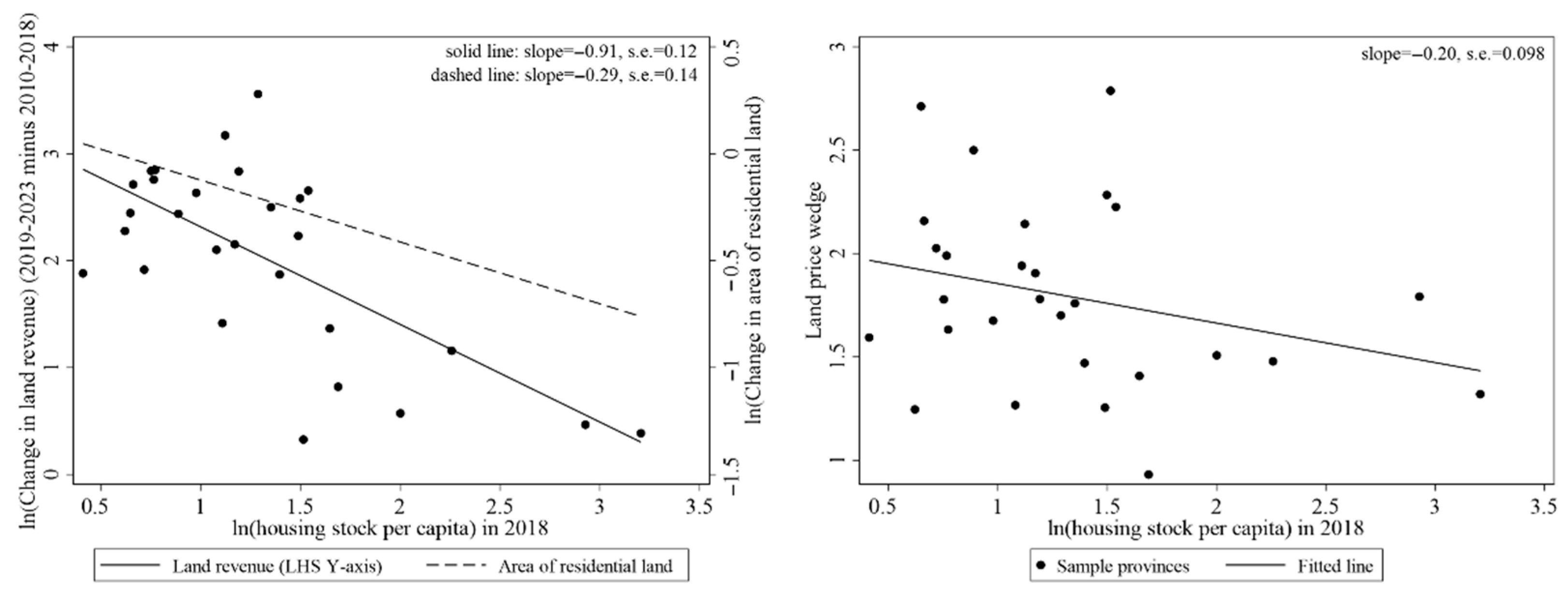
Specifically, in regions characterized by large housing inventories, local governments have prioritized destocking and risk control2, consistent with stronger regulation stringency. By contrast, in overheated markets with housing shortages, the policy priority shifts toward maintaining or even expanding residential land supply to accommodate essential demand while preventing excessive price growth. These regions are characterized by relatively lower regulatory stringency [32]. Accordingly, the stringency of housing regulation across cities is largely determined by their respective housing inventory. These distinctive regulatory measures not only cool the housing market but also have a negative impact on the land market, which is documented by extensive literature [32,33]. This differential regulatory intensity transmits distinct signals to the urban land market, thereby triggering more pronounced adjustments in regions with stringent policies. As shown in the left panel of Figure 2, per capita housing inventory is negatively associated with both land revenue and the area of residential land, indicating that cities with larger housing inventory were subject to stronger regulation stringency.
Furthermore, cities with higher per capita housing stock are typically characterized by excess housing supply, which leads to lower housing and residential land prices3. In contrast, cities with housing shortages often allocate a disproportionate share of land to the industrial sector, aimed at attracting firms and advancing promotion prospects [11,14,37]. This strategy constrains residential land supply, elevate both residential land and housing prices, and ultimately generates higher land price wedges [17,38,39]. Accordingly, regions with higher housing inventory are generally characterized by lower land price wedges. In the absence of official statistics on detailed housing inventory data at the city level in China4, we further employ the differentiated land supply strategies of local governments as a proxy for underlying housing market conditions. As shown in the right panel of Figure 2, provinces with higher housing stock per capita are likely to exhibit lower land price wedges, supporting its validity as a proxy for regulatory stringency.
Using the land transaction data, we classify land parcels into four different categories based on use type, including residential, commercial, industrial, and public land. Public land is allocated for public services, such as hospitals, parks, and schools. Public land is typically allocated through non-market or semi-market mechanisms, rendering it fundamentally incomparable with other market-transacted parcels [40]5. Moreover, as commercial land has been oversupplied in recent years [13], it has come under stringent regulatory constraints that strictly curb further allocation6. In response to housing regulations, local governments in cities with low land price wedges tend to experience more pronounced reductions in residential land supply and, concurrently, a greater reallocation of land to industrial use within the urban land quota system7. By contrast, cities with high land price wedges have greater incentives to maintain or even expand residential land to mitigate potential housing price surges8. As shown in Figure 3, cities with low price disparities experience a more rapid expansion in the proportion of industrial land following the policy intervention. We therefore hypothesize the following:
Hypothesis. 
Given fixed urban land quotas, cities with low land price wedges (stricter policy implementation) experienced significantly greater expansion in industrial land supply following housing market regulations.

3. Data and Empirical Strategy

3.1. Data

We employ a city-year panel dataset covering 266 Chinese cities at the prefecture level or above from 2010 to 2023, which merges data on land transfer, macroeconomic indicators, and geographic characteristics9. Unique administrative divisions such as leagues (Meng), autonomous prefectures (ZiZhiZhou), prefecture-level administrative regions (DiQu), and the Xinjiang Production and Construction Corps (XinJiangJianSheBingTuan) are omitted due to their distinct land supply patterns. Moreover, 24 cities undergoing significant administrative reorganization during the sample period are excluded to ensure data continuity and comparability. The six prefecture-level cities in Tibet are also omitted because of incomplete land supply data.
We obtain land transaction data from the official website of China’s land market (https://www.landchina.com/, accessed on 12 Novermber 2022), which is managed by China’s Ministry of Land and Resources. This platform provides detailed information on each land parcel, including land-use type, lot size, transaction method, sale date, sale price, address, and the designated type for land use. Although the central government began systematically recording land transaction data in 2007, discrepancies with the China Land and Resources Statistical Yearbooks were noted, particularly from 2007 to 2009. To ensure data consistency, our analysis focuses on the period from 2010 to 2023. From this period, we compile a comprehensive sample of over 2.5 million land transaction records from 266 cities. In 2018, the industrial land in our sample accounted for approximately 87.7% of China’s total industrial land transactions (in terms of land area), indicating the representativeness of our dataset for analyzing national industrial land supply. And the land transfer data used in our analysis cover roughly 82% newly developed urban construction land (converted from agricultural land) and 18% existing construction land (typically following the demolition of outdated buildings and facilities). Both categories are incorporated uniformly in our estimation. Additionally, data on provincial and city characteristics come from the China City Statistical Yearbook and CEIC (China Entrepreneur Investment Club) database.

3.2. Constructing Policy Stringency Measure

Drawing on parcel-level transactions from 2010 to 2018, we estimate the land price wedge between residential (and commercial) and industrial land using the hedonic pricing model, which assumes that the price of a land plot reflects the aggregation of a set of hedonic attributes [22]10. Equation (1) gives the hedonic pricing specification:
l n P i = α 0 + α 1 R C i + α 2 l n D i s t a n c e C e n t e r i + α 3 l n A r e a i + α 4 T r a n M e t h o d i + y e a r t + ε i t
l n P i denotes logged transaction price for land parcel i. The core explanatory variable, land use ( R C i ), is an indicator equal to one if the parcel is designated for residential or commercial uses and zero if it is designated for industrial use. To account for parcel-specific characteristics, we control for logged distance from the parcel to the city center ( l n D i s t a n c e C e n t e r i )11, logged parcel area ( l n A r e a i ), and a set of dummy variables indicating five types of land supply methods ( T r a n M e t h o d i ) (English auction (paimai), two-stage auction (guapai), allocation (huabo), negotiation (xieyi) and others, with sealed-bid auction (zhaobiao) as the reference category). Year fixed effects are also included to capture time-specific factors. The estimated coefficient α 1 , representing the price wedge between residential (and commercial) and industrial land conditional on parcel-level characteristics, serves as the core explanatory variable in the empirical model.

3.3. Econometric Specification

We employ a generalized difference-in-differences model to estimate the average marginal impacts of housing market regulation policies on land supply strategies:
Y i t = β 0 + β 1 K i × P o s t 2018 t + β X X i t + λ i + δ t + ε i t
Specifically, Yit represents industrial land supply for city (province) i in year t in absolute and proportional terms (i.e., lnIareait and Iratioit). Ki captures regulatory stringency using two indicators: (i) the log of per capita housing stock in 2018 (lnHousingStockpc2018; measured as housing stock divided by the urban residential population)12; (ii) the land price wedge estimated from Equation (1) (LandPriceWedge). We incorporate the interaction term of Ki and a post-2018 dummy that equals one for years after 2018. The coefficient β 1 is of particular interest as it indicates the regulation policies’ marginal effect on local governments’ land supply strategies. β 0 is the constant term and ε i t denotes the error term. We cluster standard errors at the city (province) level. In addition to city (province) and year fixed effects (denoted by λ i and δ t ), we also include a series of time-varying controls (X) to account for the potential impacts of local economic conditions on the results, encompassing the ratio of general budget revenue to general budget expenditure (FisPre), GDP growth rate (GDPGrowth), the proportion of the secondary industry in GDP (SecRatio), the scale of residential population (in log; lnPOP), and the total newly supplied land area (in log; lnAllarea).
In the preferred specification, we control for time-invariant city characteristics by including their interactions with year dummies. First, predetermined geographic features such as oceans, lakes, mountains, and wetlands can create relative scarcity of developable land and directly impact urban land use patterns [44]. To capture this, we include the log of developable land area per capita in 2010 (lnDevLandpc2010), calculated as the administrative area of each city net of water bodies and land with slopes greater than 15 degrees, divided by the residential population in 2010. Second, following the initiation of the US–China trade war in 2018, the Chinese central government reoriented its policy to bolster domestic industrial development, including a relaxation of constraints on industrial land supply [45,46]. To mitigate potential confounding effects from trade war, we control for the local GDP’s export and import dependency ratios on the US in 2016 (ExpDependency2016 and ImpDependency2016)13. Finally, to further account for productivity-driven disparities across regions, we control for the average industrial land-use efficiency from 2010 to 2018 (lnSIVApu2010–18). It is measured as the log of the average value added in the secondary sector per unit area over the period 2010–2018. We expect these time-invariant characteristics to influence changes in the city’s land transfer strategy after 2018. The summary statistics are reported in Table A1 of Appendix A.
We expect β 1 to be positive (negative) as regions with large housing stock (low price wedge) were likely to experience greater expansion in industrial land allocation. The empirical implication of an insignificant coefficient is that the growth in industrial land supply was statistically indistinguishable across cities after the policy. In other words, cities collectively expanded supply, maintaining the pre-existing distribution of industrial land shares. Moreover, to identify the impact of the regulatory policy on land supply, we exploit cross-city variations in land price wedges before 2018. While price wedges are not necessarily exogenous, the 2018 housing regulation policy was centrally mandated and thus not responsive to local land market conditions, allowing us to interpret post-policy changes in land supply strategies as independent of preexisting local market fundamentals. We therefore interpret these changes in land supply strategies as a causal effect of regulatory policy. To address this concern that confounding factors might drive our results, we specifically test for the presence of observable pre-trends in the years prior to the policy implementation using an event study framework.
To further examine the policy’s dynamic impact on local land supply strategies, we provide evidence on the timing of the change in industrial land-supply intensity relative to the policy using an event-study specification. The regression model is as follows:
Y i t = β 0 + k   =   8 5 β k K i × t i m e k + β X X i t + λ i + δ t + ε i t ,
where 2018 (k = 0) is the benchmark. In our analysis, k runs from 8 (i.e., 2010 minus 2018), up to eight years prior to the policy, to 2023, up to five years following the housing regulation’s initiation. Other model settings are the same as in Equation (2).

4. Results

4.1. Baseline Results

Before presenting the baseline results, we conduct a series of provincial-level regressions to assess whether the land price wedge is a valid proxy for regulatory tightness. We first use housing stock per capita in 2018 as a proxy for regulatory stringency, and estimate Equation (2) at the province level to examine its effect on industrial land supply (columns 1 and 2 of Table 1). Moreover, housing stock per capita is highly correlated with the land price wedge, as discussed previously (detailed in Section 3.2). We therefore re-estimate the hedonic model in Equation (1) at the province level to obtain the land price wedge and incorporate it into the regressions following Equation (2) (columns 3 and 4)14. Similarly, we further replace the dependent variables with their city-level counterparts and run corresponding regressions (columns 5–8). Collectively, we find that all the coefficients are statistically significant, indicating that provinces with large housing stock or low land price wedges (stronger regulatory stringency) are more likely to expand industrial land supply following the housing market regulation.
Our analysis of housing stock is constrained by the unavailability of city-level data. Given its negative association with per capita housing stock (detailed in Section 3.2), the land price wedge serves as a proxy for regulatory stringency. This allows us to estimate Equation (2) at the city level to capture city-specific characteristics at a more refined level. Columns 1 and 2 of panel A in Table 2 indicate that cities with stricter policy implementation (lower price wedges) experience significantly larger increases in both the proportion and area of industrial land supply after 2018. The findings align with the patterns illustrated in the right panel of Figure 3. This reallocation corresponds to a reduction in residential land supply (columns 3 and 4), whereas the commercial and total land supply remained statistically unchanged (columns 5–7). Specifically, for a city with an average land price wedge (mean = 1.217), the policy increases the industrial land share by approximately 4.7 percentage points. Panel B further includes the interactions between time-invariant confounding factors and time dummies, and the results are highly consistent with those in Table 1. Accordingly, under a fixed total land supply quota15, housing regulations result in a reorganization of urban land use, increasing industrial land supply at the expense of residential land allocation.
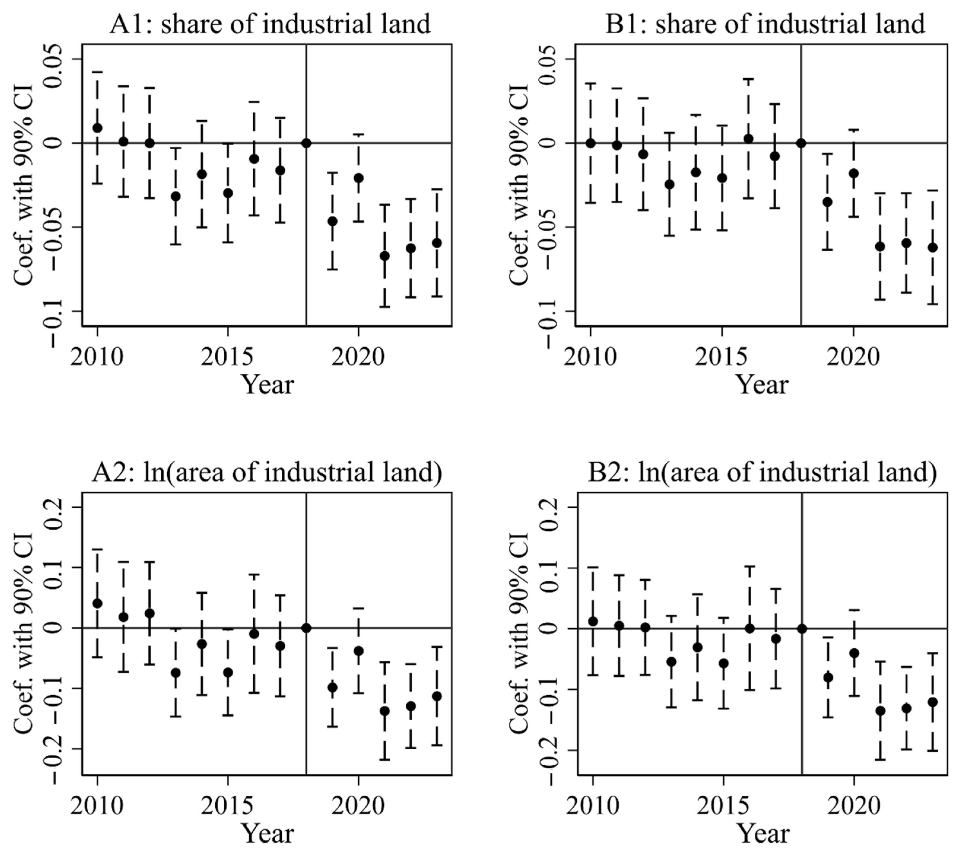
The event study estimates presented in Figure 4 further support this substitution pattern. The figure displays the estimated coefficients from Equation (3) along with 90% confidence intervals. Panel A controls for city-level characteristics and two-way fixed effects, while panel B further augments the model with interactions between year dummies and time invariant factors, namely the share of exports to the US in GDP in 2016, the share of imports from the US in GDP in 2016, the log of developable land per capita in 2010, and the log of average industrial land-use efficiency from 2010 to 2018. Across all specifications, when using either the proportion of industrial land or the log of industrial land area as dependent variables, the coefficients are statistically significant and negative after 2018. These findings indicate that the regulatory policy leads to larger increases in industrial land supply among cities with lower price wedges, providing preliminary support for our hypothesis.

4.2. Robustness Checks

This subsection conducts a series of sensitivity checks to verify the robustness of our baseline estimates. Firstly, public land is allocated through non-market or semi-market mechanisms, rendering it fundamentally incomparable with market-determined residential, commercial, and industrial parcels [40]. We therefore exclude it from the baseline regressions and include it in the robustness checks to address potential substitution between public and residential land. Following the specification in Equation (2), we replace the dependent variable with the share of public land, the log of public land area, and the log of total land supply including public land, respectively. As reported in Table A3 of Appendix A (columns 1–3), coefficients on the share and area of public land, as well as the total land supply inclusive of public land, are statistically insignificant. The above findings suggest that the exclusion of public land does not bias the baseline estimates and alleviates concerns regarding substitution with residential land.
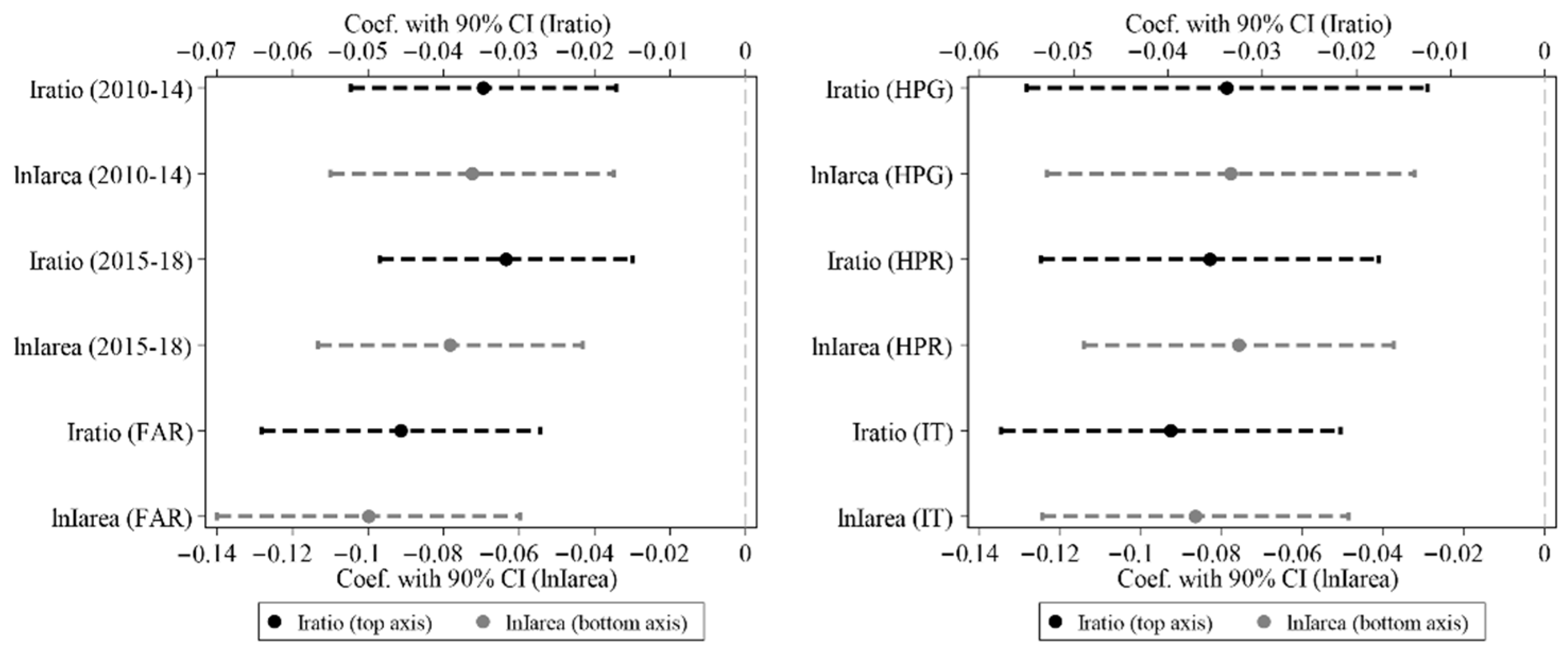
Secondly, the price wedge between residential (and commercial) and industrial land used in the baseline regressions is estimated from micro-level transaction data spanning 2010–2018. To address potential measurement errors, we re-estimate the hedonic price model (Equation (1)) under alternative specifications that replace the stringency measure with plausible alternatives. Specifically, we restrict the sample to 2010–2014 (lines 1 and 2 of left panel in Figure 5), 2015–2018 (lines 3 and 4), and the entire 2010–2018 period, with additional controls for the floor area ratio (FAR) (lines 5 and 6)16. Overall, the results are statistically consistent across all specifications, confirming the robustness of the baseline estimates.
Thirdly, the Political Bureau of the CPC Central Committee in July 2018 explicitly called for “resolutely curbing the rise in housing prices”, marking a critical turning point that shifted market expectations from a trajectory of moderate appreciation to an anticipated decline17. Consequently, cities experiencing rapid housing price growth are likely to impose stricter regulations, and may display larger price wedges due to elevated housing and land values, creating a potential mismatch between the land price wedge and regulatory intensity. To alleviate the concern, we employ an established city-tier classification based on past house price growth [47], which categorizes cities into four tiers, with first- and second-tier cities typically experiencing the highest appreciation. As reported in lines 1–2 of the right panel in Figure 5, the results remain largely unchanged.
Fourthly, during the 2010–2011 period, the Chinese government enacted a series of stringent housing market measures, notably the Home Purchase Restrictions (HPR) [24,27,28]. Although HPR may have impacted the housing and residential land market in subsequent years, the event-study results presented in Figure 4 show parallel pre-trends prior to the intervention, which helps alleviate this concern about anticipatory effects. To further mitigate the concern, we exclude the 2010–2011 period as a robustness check. The results, reported in lines 3–4 of the right panel in Figure 5, remain unchanged, validating the robustness of our findings and indicating that the earlier HPR does not confound the identification of post-2018 policy effects.
Fifthly, although new industrial land is not concentrated in higher productivity areas18, an alternative mechanism related to industrial transfer may be at work. High factor costs in major cities have a crowding-out effect on the manufacturing sector, encouraging firms to relocate from core to peripheral cities [48]19. Peripheral cities adjacent to core cities are favored because of their desirable accessibility and lower factor costs. Therefore, this type of peripheral city may have experienced rapid industrial land expansion since 2018. Accordingly, we augment Equation (2) with an interaction between the post-2018 dummy and a dummy variable indicating whether a peripheral city is geographically adjacent to a core city. Our analysis reveals no statistically significant differential in industrial land expansion between peripheral cities, regardless of their proximity to a core city (coefficients are not reported). Moreover, the coefficients and magnitudes of the key explanatory variables remain robust, providing evidence against the market-led industrial transfer mechanism (lines 5–6 of the right panel in Figure 5).
Lastly, large-scale demolition has been a salient feature of China’s urban transformation, with first-order implications for housing supply. According to the 2013 Chinese Household Income Project, 13.3% of urban households had experienced demolition by that year [49,50]. This process intensified between 2015 and 2019 under the resettlement-based shantytown redevelopment program (CR_SRP), which combined demolition with redevelopment and was implemented with varying intensity across cities. The program often combined demolition with cash compensation and has been shown to stimulate local real-estate activity [49,51]. To formally assess whether demolition could be driving our results, we construct a city-level measure of CR_SRP intensity as the ratio of cash-resettlement units to urban population in 2016 (in log), the peak year of cash resettlement20. We then augment Equation (2) by interacting the post-2018 indicator with the city-level CR_SRP intensity. The coefficients on this interaction, reported in Table A5 of Appendix, are not statistically significant, and the magnitudes and significance of our key explanatory variables are largely unchanged. These results provide evidence against a demolition-driven mechanism behind our main findings.

4.3. Heterogeneity Effects

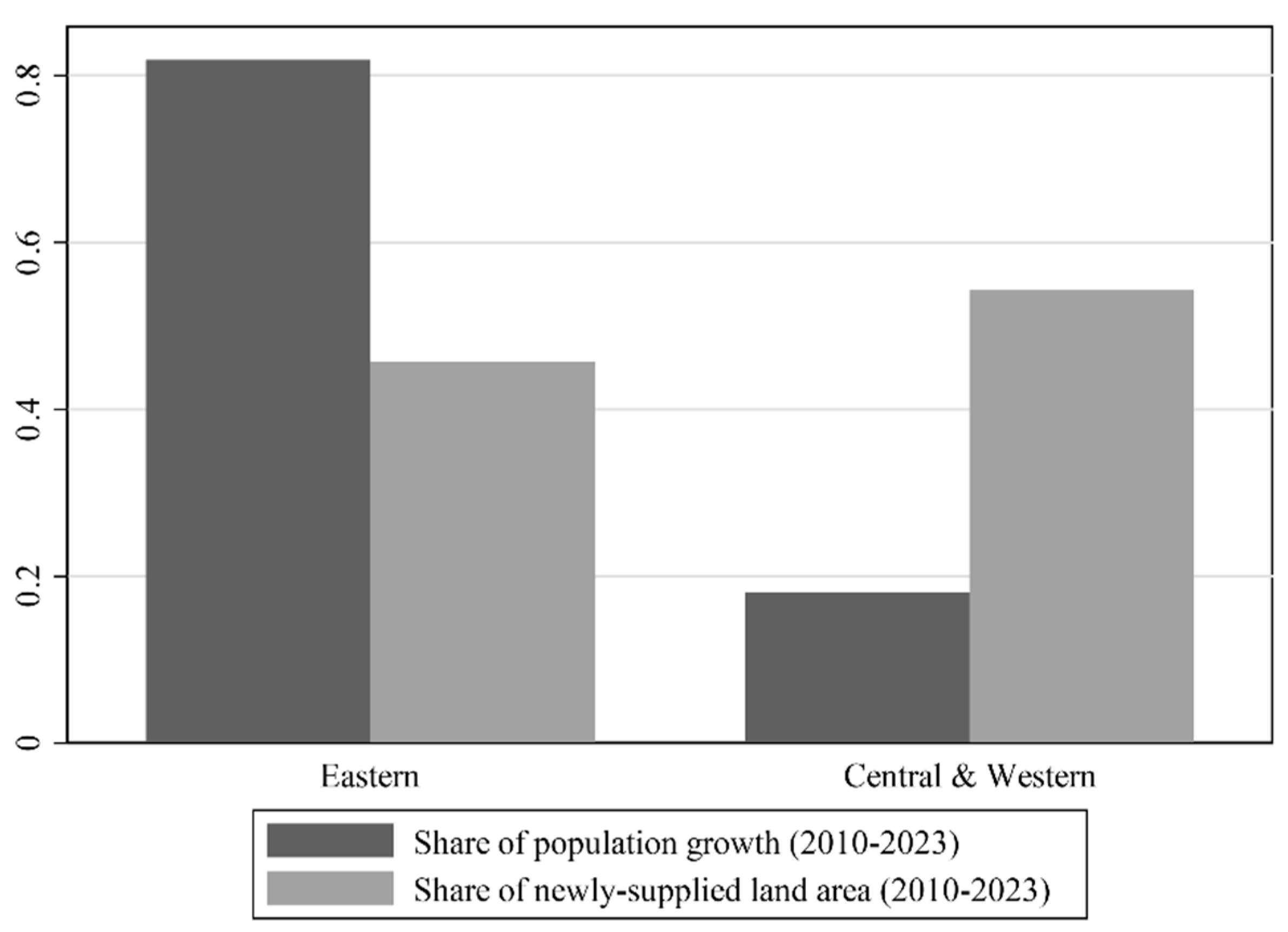
Since 2003, China’s inland-favoring land allocation policy has distributed a growing share of land quotas toward the central and western regions, tightening land quota constraints in the east [52,53]. This constitutes a significant misallocation, given that the economic value of urban land is substantially higher in the developed eastern regions than in their less developed central-western counterparts. Figure 6 compares the eastern and central-western regions in terms of their respective shares of national population growth and new land supply from 2010 to 2023. The central-western regions received a majority (54.3%) of the newly supplied land area, whereas the eastern regions accounted for a disproportionately larger share (81.9%) of national population growth, reflecting a pronounced disparity.
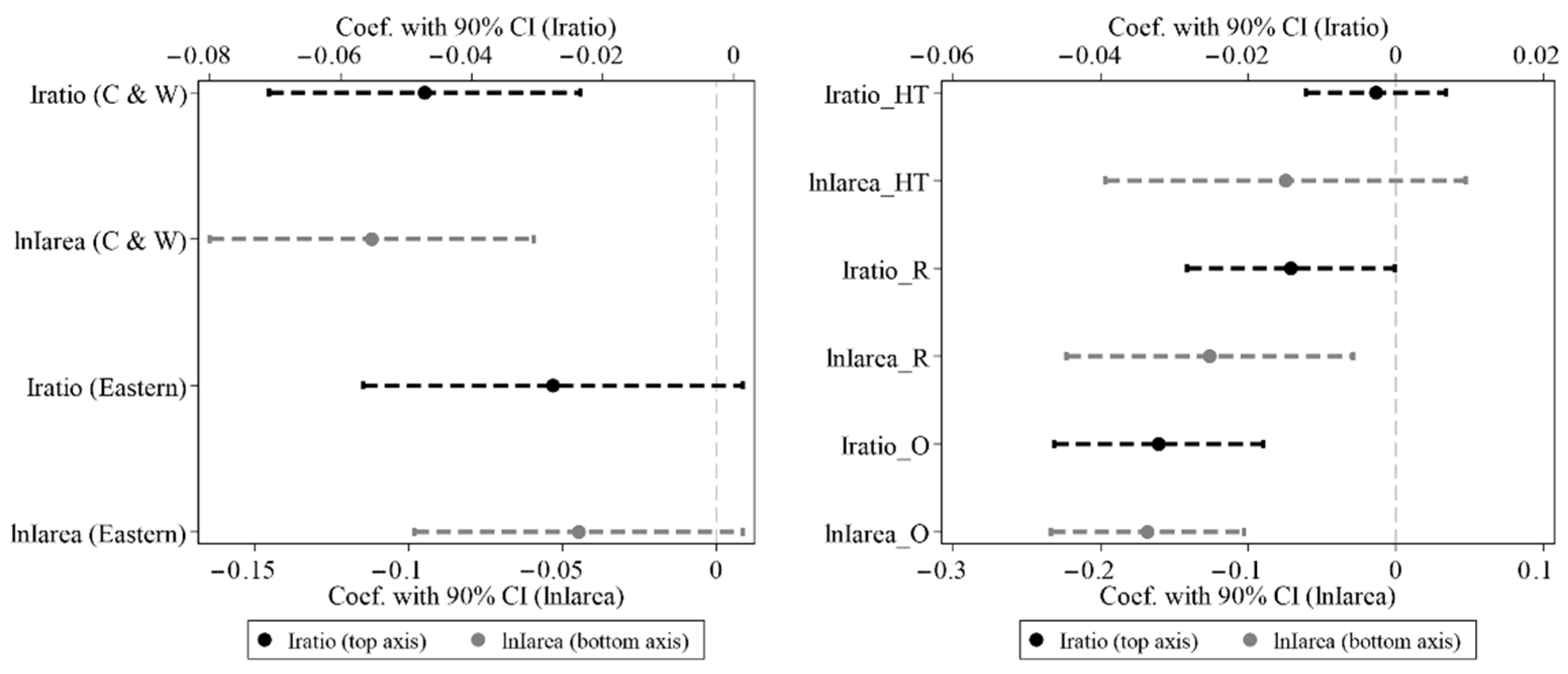
Accordingly, in cities with more binding land supply constraints, the higher opportunity cost of reallocating land dampens the impact of housing regulations on land use [7]. Conversely, cities with less stringent land quotas may exhibit stronger substitution effects between residential and industrial uses under the fixed urban land quota system. We thus anticipate the relaxation of quota limits in central and western regions to manifest as stronger industrial land expansion there. To account for this regional heterogeneity, we estimate separate regressions for the eastern and central-western regions, with the results reported in the left panel of Figure 7. As expected, the coefficients are statistically significant for the central-western regions (lines 1–2) but insignificant for the eastern region (lines 3–4). These results indicate a more pronounced reallocation from residential to industrial land use in central and western regions, aligning with their less stringent land quota constraints.
Building on the preceding evidence that regulation induces larger increases in industrial land where land supply is less constrained, we further investigate which types of industrial land benefit from this expansion. Industrial land is categorized into three mutually exclusive types: high-tech, restricted, and other industries. High-tech involves intensive technology input and high value added production. “Restricted” industries comprise sectors designated as highly polluting or suffering from overcapacity, while the “Other” category captures the rest of industrial uses21.
We estimate separate effects for each land category. For high tech industrial land, lines 1, 2 in the right panel of Figure 7 show no significant effect, suggesting the policy did not meaningfully promote land supply for advanced manufacturing22. By contrast, lines 3–6 reveal significant effects for both restricted and other industrial land. These findings imply that the housing regulation policy, particularly in cities with lower land price wedges, shifted land toward pollution-intensive and general industrial sectors rather than high-tech industries. The evidence points to a reallocation motivated by short term quota targets rather than strategic industrial upgrading.

4.4. Further Analysis

Our findings by far indicate that cities under stricter housing market regulation experience significantly larger post-2018 increases in industrial land allocation. We anticipate that policy-induced shifts in industrial land supply may have implications for the economic composition. Consequently, we re-estimate Equation (2) with alternative outcome variables: the number of industrial enterprises (in log)23, the secondary industries’ value added per capita (in log), the proportion of value-added in the secondary industry to that in the tertiary sector, and an index of industrial land distortion (measured as the ratio of the share of newly supplied industrial land to the share of secondary industry in GDP)24 [55]. The results, presented in Figure 8, reveal that cities with greater industrial land allocation see no concurrent growth in the number of industrial enterprises, per capita value added in the secondary sector, improvements in industrial structure, or land use efficiency (lines 1–4 of Figure 8). Notably, the positive coefficients in lines 2–3 indicate that cities allocating more land to industrial uses experienced larger declines in both secondary-sector value added per capita and in the industrial structure. Taken together, these results imply that the expansion of industrial land in these cities has not been accompanied by corresponding gains in economic performance, pointing to a potential inefficiency in land resource allocation.

5. Concluding Remarks

Using a panel of city-year level observations from 2010 through 2023, this study presents empirical evidence demonstrating how housing market policy interventions influence local governments’ land supply strategies in China. Our findings reveal that this macroeconomic regulation policy, aimed at curbing excessive housing market expansion, restricts the scale of residential land supply without affecting total land supply. The policy-induced contraction in residential land leads to increased allocations for industrial use, particularly in cities that enforced the regulation more stringently, while its effects on commercial and public land remain not statistically significant, consistent with our hypothesis. Moreover, the implementation of policy initiatives has been more stringent in cities with a relatively abundant land supply, resulting in a more pronounced expansion of industrial land allocation in these regions, which reveals a significant substitution mechanism between residential and industrial land uses. Additionally, we find that the expansion of industrial land fails to yield short-term improvements in output or firm entry, suggesting inefficient reallocation across land uses. Based on the empirical findings discussed above, the following policy implications are proposed to enhance the efficiency of land use regulation and foster sustainable urban development:
Firstly, to introduce compositional constraints within aggregate land quotas. The key finding of a substitution mechanism between residential and industrial land, occurs under binding city-level quotas, as existing policies lack explicit restrictions on the composition of land use types within these quotas. Inflexible regulatory frameworks may exacerbate frictions in land markets, whereas aligning land allocations with local economic conditions could improve land use efficiency. Specifically, this could be achieved by setting minimum allocation requirements for residential land in cities facing housing shortages and maximum caps for industrial land in regions with evidence of overcapacity or lower land-use efficiency.
Secondly, to establish a performance-based management system for industrial land. Given that the expansion of industrial land fails to improve short-term economic performance, allocations should be conditioned on observable outcomes. A dynamic assessment system for industrial land is essential for evaluating parcels based on investment intensity, tax revenue generation, job creation per unit of land area, etc. Plots that consistently underperform would face escalating remedies, such as penalties, recapture, or conversion to other uses (e.g., residential or commercial), which creates incentives for efficient utilization and alleviates residential land scarcity without expanding the total urban footprint.
Thirdly, to liberalize the urban land market and change the monopolistic position of local governments. The current regime encourages strategic reallocation across uses, as evidenced by the substitution mechanism identified in this study. Introducing market mechanisms, such as allowing rural collective construction land to enter the market or enabling land use rights transfers between private entities, would help align land supply with local fundamentals. These reforms could enhance land use efficiency in China’s urban land market and offer guidance for other developing economies confronting regulatory rigidity.
We focus on short-term adjustments in land supply, an immediate policy response observable within our sample period ending in 2023. A critical avenue for future work is to quantify the long-run general equilibrium effects, particularly through inter-regional factor mobility. Examining how labor and capital flows respond to, and subsequently reshape, the land-use reallocations we document would provide a more comprehensive view of the policy’s aggregate economic impact. Exploring these dynamic adjustments across markets remains a challenging but promising direction for subsequent work.

Author Contributions

Conceptualization, H.X. and S.L.; Methodology, H.X., S.L. and W.Z.; Software, S.L.; Validation, H.X. and S.L.; Formal analysis, H.X., S.L. and W.Z.; Investigation, H.X., S.L. and W.Z.; Resources, H.X.; Data curation, S.L. and W.Z.; Writing—original draft, H.X. and S.L.; Writing—review and editing, H.X. and S.L.; Visualization, H.X. and S.L.; Supervision, H.X.; Project administration, H.X. and S.L.; Funding acquisition, H.X. All authors have read and agreed to the published version of the manuscript.

Funding

This work was supported by the National Natural Science Foundation of China under Grant [number 72173038].

Data Availability Statement

The data presented in this study are available on request from the corresponding author. The data are not publicly available due to privacy.

Conflicts of Interest

The authors declare no conflicts of interest.

Appendix A

Table A1. Summary statistics at the city level.
VariableMeanS.D.Min.Max.Obs.
Panel data
Iratio0.5230.1600.0060.9763680
Iarea (in hectare)476.896434.7881.1204118.2523680
Rratio0.3550.1380.0060.8563680
Rarea (in hectare)328.263336.1270.0854315.0993680
Cratio0.1220.08100.7473680
Carea (in hectare)106.481116.1301553.8893680
Allarea (in hectare)911.641797.71914.5517800.3313680
FisPre0.4530.2230.0562.1443680
GDPGrowth0.0820.084−0.6320.4793680
SecRatio0.4500.1120.1070.8973680
POP (in thousand)45,459.92935,453.5422318.530321,3343680
SecTerRatio1.1830.6300.1579.1963402
NFirm1315.7061631.6132013,8443155
SVApc (thousand Yuan/person)26.14419.1301.451179.2023680
Cross-sectional data
LandPriceWedge1.2170.520−0.3192.618266
DevLandpc2010 (in sq.m)2531.2976721.25794.80083,740.540266
ExpDependency20160.0160.02900.202266
ImpDependency20160.0040.01000.074266
SIVApu2010–18
(billion Yuan/hectare)
0.1970.1250.0221.206266
Notes: Data on land transactions come from the website of the “China Land Market” (http://www.landchina.com/, accessed on 12 November 2022). Data on city characteristics come from the China City Statistical Yearbook, including the ratio of general budget revenue to general budget expenditure (FisPre), GDP growth rate (GDPGrowth), the ratio of the value added of the secondary industry to local GDP (SecRatio), residential population (POP), the proportion of value added in the secondary industry to that in the tertiary sector (SecTerRatio), the number of industrial enterprises above designated size (NFirm), the value added of secondary industry per capita (SVApc), and average value added of secondary industry per unit area in 2010–2018 (SIVApu2010–18). Data on the ratio of exports (imports) to the US relative to GDP (ExpDependency2016) (ImpDependency2016) come from China’s General Administration of Customs. Data on developable land per capita (DevLandpc2010) come from the ASTER Global Digital Elevation Model V003 and China Land Cover Dataset.
Table A2. Summary statistics at the province level.
VariableMeanS.D.Min.Max.Obs.
Panel data
IratioProv0.5090.1240.0520.862392
IareaProv (in hectare)4477.0603533.84316.29819,582.678392
AllareaProv (in hectare)8532.5066679.777176.85135,968.719392
FisPreProv0.4990.1970.1841.294392
GDPGrowthProv0.0840.074−0.3080.297392
SecRatioProv0.4300.0990.1490.673392
POPProv (in thousand)423,945.920279,184.81027,315.7811,270,600392
Cross-sectional data
HousingStockpc2018 (sq.m/person)0.4890.5130.1512.46728
LandPriceWedgeProv1.7950.4510.9312.78828
Notes: Data on land transactions come from the website of the “China Land Market” (http://www.landchina.com/, accessed on 12 November 2022). Data on housing stock (HousingStockpc2018) come from the CEIC (China entrepreneur Investment Club) database. Data on provincial characteristics come from the China City Statistical Yearbook, including the ratio of general budget revenue to general budget expenditure (FisPreProv), GDP growth rate (GDPGrowthProv), the ratio of the value added of the secondary industry to local GDP (SecRatioProv), and residential population (POPProv).
Table A3. Robustness checks with public land included.
(1)(2)(3)
PTratiolnPTarealnAllareaPT
LandPriceWedge × Post2018−0.020−0.0520.015
(0.012)(0.038)(0.040)
ControlsYYY
City and Year FEsYYY
Observations368036803680
R-squared0.3520.6780.170
Notes: All specifications align with Equation (2). The key independent variable is the interaction between the time dummy and the land price wedge (LandPriceWedge). The dependent variables are the share of public land in total land supply (PTratio), the logged public land area (lnPTarea), and the logged total land supply including public land (lnAllareaPT), respectively. Column 3 excludes the logged total land supply including public land (lnAllareaPT) from controls as it serves as the dependent variable in the regression. Standard errors (clustered at the city level) are in parentheses.
Table A4. Robustness checks with expectation effects controlled.
(5)(6)
IratiolnIarea
LandPriceWedge
× Post2018
−0.038 ***−0.085 ***
(0.013)(0.027)
LandPriceWedge0.00240.0060
× Year2016(0.018)(0.045)
LandPriceWedge−0.0045−0.014
× Year2017(0.018)(0.043)
LandPriceWedge0.0120.015
× Year2018(0.015)(0.041)
ControlsYY
City and Year FEsYY
Observations36803680
R-squared0.1810.734
Notes: All specifications align with Equation (2). The key independent variable is the interaction between the time dummy and the land price wedge (LandPriceWedge). The dependent variables are the share of industrial land in total land supply (Iratio), and the log of the area of industrial land (lnIarea), respectively. LandPriceWedge × Year2016 (Year2017; Year2018) denotes the interaction term between the land price wedge and time dummies for 2016, 2017 and 2018. *** p < 0.01. Standard errors (clustered at the city level) are in parentheses.
Table A5. Robustness Check for Demolition Effects (CR_SRP).
(1)(2)
IratiolnIarea
LandPriceWedge × Post2018−0.032 ***−0.071 ***
(0.012)(0.026)
CR_SRP intensity × Post20180.000860.012
(0.0052)(0.011)
ControlsYY
City and Year FEsYY
Observations29402940
R-squared0.1910.737
Notes: All specifications align with Equation (2). The key independent variable is the interaction between the time dummy and the land price wedge (LandPriceWedge). The dependent variables are the share of industrial land in total land supply (Iratio) and the log of the area of industrial land (lnIarea). CR_SRP intensity × Post2018 denotes the interaction term between the post-2018 dummy and intensity of the CR_SRP, which is measured as the ratio of the number of a city’s cash resettlement-based shantytown redeveloped housing units to its urban population in 2016 (in log). Our analysis of CR_SRP intensity is based on a sample of 212 cities for which data are available. *** p < 0.01. Standard errors (clustered at the city level) are in parentheses.
Table A6. Robustness check for high-tech industrial land supply using QMLE model.
(1)
Iarea_HT
LandPriceWedge × Post2018−0.0084
(0.062)
ControlsY
City and Year FEsY
Observations3680
Pseudo R-squared0.786
Notes: The specification employs a Poisson quasi-maximum likelihood (QMLE) model, where control variables include fiscal pressure (FisRev), GDP growth rate (GDPGrowth), the log of residential population (lnPOP), industrial structure (SecRatio), and the log of total land supply (lnAllarea). Two-way fixed effects are also included. The key independent variable is the interaction between the time dummy and the land price wedge (LandPriceWedge). The dependent variable is the area of high-tech industrial land (Iarea_HT). Standard errors (clustered at the city level) are in parentheses.
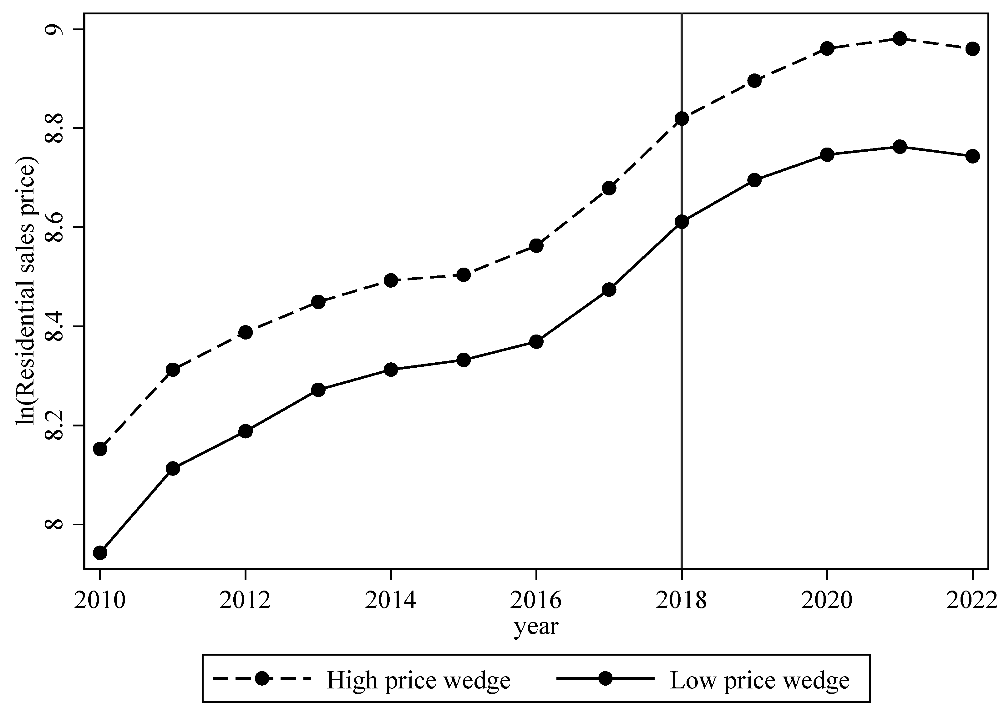
Figure A1. The log of annual residential sales prices from 2010 to 2022 by category. Notes: The figure illustrates the log of housing prices by city type from 2010 to 2022 (annual average).
Land 14 02228 g0a1

Notes

1.
Housing prices maintained an upward trend with no notable shift around 2018 (Figure A1 of Appendix A), implying that the regulation policy induced simultaneous leftward shifts in both the demand and supply curves for residential property.
2.
Housing regulations were also applied to cities experiencing rapid price appreciation, which is specifically designed to curb excessive growth. Our baseline results remain robust to the exclusion of these cities (detailed in Section 4.2).
3.
Housing prices and residential land prices are jointly determined in classic urban models [34,35,36].
4.
City-level housing stock The baseline results remain robust if public land is included (detailed in Section 4.2) statistics with official coverage are not available in China. Related reporting can be found at: https://news.sina.cn/2022-08-14/detail-imizmscv6127707.d.html?utm_source=chatgpt.com, accessed on 14 August 2022 and https://kandian.ke.com/detail/MjY3MjM4NzI=.html?beikefrom=pc_kd_index, accessed on 5 August 2022.
5.
The baseline results remain robust if public land is included (detailed in Section 4.2).
6.
Local governments tend to prioritize industrial land because of its perceived role in attracting investment and fostering growth, whereas they take a more cautious stance toward commercial land. Industrial parcels are often subsidized or allocated strategically to attract firms, while commercial land is subject to stricter market discipline and administrative oversight, reflecting concerns about speculative activity and inefficient land use.
7.
Details on the estimation of the land price wedge are provided in Section 3.2.
8.
In 2018, the Ministry of Housing and Urban-Rural Development pointed out that in hotspot cities, the share of residential land in total urban construction land should be increased, with residential land accounting for no less than 25 percent.
9.
Our analysis uses the prefecture-level city as the primary spatial unit, consistent with extensive prior research on China’s urban and regional economies [17,41,42,43]. In China, a prefecture-level city encompasses a central urban core (typically composed of several urban districts (shiqu)) as well as surrounding rural counties and towns. While this administrative definition differs from the functional definition of “city” often employed in the context of other countries, it aligns with the level of government that makes land-supply decisions central to our analysis.
10.
This pattern is consistent with substantial disparity in land transaction prices across uses, as industrial land is generally transacted at considerably lower prices than those for residential and commercial uses [39]. Accordingly, we estimate price wedges for residential and commercial land relative to industrial land.
11.
For each parcel in our sample, we calculate the distance to municipal government building, which is typically located in the traditional central business district.
12.
Due to the absence of city-level housing stock data, specifications involving housing stock per capita are estimated at the province level.
13.
ExpDependency2016 and ImpDependency2016 are based on each city’s imports and exports to the US in 2016, relative to the city’s GDP in that year. We can only access it from China’s 2016 customs data and assume that these two trade dependence variables to be relatively stable between 2010 and 2018.
14.
Table A2 presents summary statistics at the province level.
15.
Upper-level governments reward jurisdictions that fully utilize their annual land quotas with additional allocations in the following year.
16.
Due to substantial missing data on FAR, the baseline estimates of price wedges do not control for this variable.
17.
In addition, the government first introduced the principle that “houses are for living in, not for speculation” in 2016, which may have shaped market expectations. The event study analysis in Figure 4 helps alleviate this concern. As an additional check, we control for the interaction between the land price wedge and time dummies for 2016, 2017 and 2018. The results, reported in Table A4 of the Appendix A, show that the main results remain robust.
18.
The coefficient of industrial land use efficiency is not statistically significant in panel B of Table 2 (coefficients of controls are not reported and results are available upon request).
19.
Core cities are defined as those that either demonstrate exceptional performance in advanced manufacturing (according to a report by the China Center for Information Industry Development, a public institution under China’s Ministry of Industry and Information Technology, in 2018) or hold a higher administrative status than the typical prefecture-level city, including provincial cities (ZhiXiaShi), cities granted independent planning status (JiHuaDanLieShi) at the subprovincial level, and provincial capitals (ShengHui). This classification yields 56 core cities and 210 peripheral cities.
20.
The count of resettlement units is hand-collected from Statistical Bulletins on National Economic and Social Development, government work reports, and official releases by provincial and municipal agencies (Housing and Urban-Rural Development; Planning and Natural Resources). Because systematic disclosure largely ceased after 2016, we use the 2016 intensity as a proxy for overall program intensity during 2015–2019.
21.
“High-tech” refers to industrial land used for pharmaceutical manufacturing, transportation equipment manufacturing, electronic equipment manufacturing, instrumentation manufacturing, and special equipment manufacturing. “Restricted” pertains to sectors identified as high-pollution or suffering from overcapacity, as specified by the State Environmental Protection Administration (2008) and the State Council of the People’s Republic of China (2013), which include sugar and food product manufacturing; beverage production; textile manufacturing; leather tanning and dressing; paper and paperboard manufacturing; refined petroleum production; basic chemicals, fertilizers, pesticides, cleaning products, and pharmaceutical manufacturing; rubber tire and tube manufacturing; metal treatment and coating; nonmetallic mineral product manufacturing; iron and steel casting; precious and other nonferrous metal manufacturing; and ship building.
22.
With over 200 zeros in high-tech industrial land area, an average treatment effect in logs is not well-defined. We therefore re-estimate the specification from the second line of the right panel in Figure 7 using Poisson pseudo-maximum likelihood model [54] and results remain largely unchanged (Table A6 of the Appendix A).
23.
Industrial enterprise above designated size refers to those industrial enterprises with annual main business income of more than 20 million Chinese Yuan.
24.
Such a metric facilitates an assessment of the alignment between land allocation and local economic structure. In industrialized cities, this ratio would be expected to approximate one. Conversely, in cities oriented towards services or agriculture, a value significantly greater than one would indicate an excessive allocation of industrial land relative to economic fundamentals, suggesting potential resource misallocation.

References

  1. Lucas, R.E.; Rossi-Hansberg, E. On the internal structure of cities. Econometrica 2002, 70, 1445–1476. [Google Scholar] [CrossRef]
  2. De Vor, F.; De Groot, H.L. The impact of industrial sites on residential property values: A hedonic pricing analysis from the Netherlands. Reg. Stud. 2011, 45, 609–623. [Google Scholar] [CrossRef]
  3. Koster, H.R.; Rouwendal, J. The impact of mixed land use on residential property values. J. Reg. Sci. 2012, 52, 733–761. [Google Scholar] [CrossRef]
  4. Duranton, G.; Puga, D. Urban land use. In Handbook of Regional and Urban Economics; Elsevier: Amsterdam, The Netherlands, 2015; Volume 5, pp. 467–560. [Google Scholar]
  5. Shertzer, A.; Twinam, T.; Walsh, R.P. Zoning and the economic geography of cities. J. Urban Econ. 2018, 105, 20–39. [Google Scholar] [CrossRef]
  6. Djankov, S.; Glaeser, E.; Perotti, V.; Shleifer, A. Property rights and urban form. J. Law Econ. 2022, 65, S35–S64. [Google Scholar] [CrossRef]
  7. Xu, H. Commercial-to-residential land-use conversion and residential recentralization in large cities. Can. J. Econ. 2023, 56, 306–338. [Google Scholar] [CrossRef]
  8. Xu, C. The fundamental institutions of China’s reforms and development. J. Econ. Lit. 2011, 49, 1076–1151. [Google Scholar] [CrossRef]
  9. Wang, Z.; Zhang, Q.; Zhou, L.A. Career incentives of city leaders and urban spatial expansion in China. Rev. Econ. Stat. 2020, 102, 897–911. [Google Scholar] [CrossRef]
  10. Fu, S.; Xu, X.; Zhang, J. Land conversion across cities in China. Reg. Sci. Urban Econ. 2021, 87, 103643. [Google Scholar] [CrossRef]
  11. Chen, T.; Kung, J.S. Do land revenue windfalls create a political resource curse? Evidence from China. J. Dev. Econ. 2016, 123, 86–106. [Google Scholar] [CrossRef]
  12. He, Z.; Nelson, S.T.; Su, Y.; Zhang, A.L.; Zhang, F. Zoning for profits: How public finance shapes land supply in China. Natl. Bur. Econ. Res. 2022, w30504. [Google Scholar] [CrossRef]
  13. Zhang, L.; Lu, M.; Liu, Y. Tax incentives and supply structure of commercial and residential land. China Econ. Q. 2022, 22, 1425–1446. (In Chinese) [Google Scholar]
  14. Tian, W.; Wang, Z.; Zhang, Q. Land allocation and industrial agglomeration: Evidence from the 2007 reform in China. J. Dev. Econ. 2024, 171, 103351. [Google Scholar] [CrossRef]
  15. Lin, G.C. Reproducing spaces of Chinese urbanisation: New city-based and land-centred urban transformation. Urban Stud. 2007, 44, 1827–1855. [Google Scholar] [CrossRef]
  16. Jiang, S.; Miao, J.; Zhang, Y. China’s housing bubble, infrastructure investment, and economic growth. Int. Econ. Rev. 2022, 63, 1189–1237. [Google Scholar] [CrossRef]
  17. Henderson, J.V.; Su, D.; Zhang, Q.; Zheng, S. Political manipulation of urban land markets: Evidence from China. J. Public Econ. 2022, 214, 104730. [Google Scholar] [CrossRef]
  18. Tang, M. Industrialize with tax structure change: Agricultural tax abolition and local industrial growth in China. China Econ. Rev. 2025, 90, 102339. [Google Scholar] [CrossRef]
  19. Xiao, J.; Zhang, Q.; Knight, B.; Gong, L. Political budget cycles, government size, and the allocation of public funds: Evidence from prefectures in China. China Econ. Rev. 2025, 94, 102542. [Google Scholar] [CrossRef]
  20. Sun, W.; Song, Z.; Xia, Y. Government-enterprise collusion and land supply structure in Chinese cities. Cities 2020, 105, 102849. [Google Scholar] [CrossRef]
  21. Xu, G.; Shen, Z.; Si, R. Anti-corruption shocks, political incentives, and regional economic development in a developmental state. J. Dev. Econ. 2025, 179, 103606. [Google Scholar] [CrossRef]
  22. Zhang, J.; Fan, J.; Mo, J. Government intervention, land market, and urban development: Evidence from Chinese cities. Econ. Inq. 2017, 55, 115–136. [Google Scholar] [CrossRef]
  23. Glaeser, E. Triumph of the City; Penguin Press: New York, NY, USA, 2011. [Google Scholar]
  24. Du, Z.; Zhang, L. Home-purchase restriction, property tax and housing price in China: A counterfactual analysis. J. Econom. 2015, 188, 558–568. [Google Scholar] [CrossRef]
  25. Glaeser, E.; Huang, W.; Ma, Y.; Shleifer, A. A real estate boom with Chinese characteristics. J. Econ. Perspect. 2017, 31, 93–116. [Google Scholar] [CrossRef]
  26. Li, V.J.; Cheng, A.W.W.; Cheong, T.S. Home purchase restriction and housing price: A distribution dynamics analysis. Reg. Sci. Urban Econ. 2017, 67, 1–10. [Google Scholar] [CrossRef]
  27. Sun, W.; Zheng, S.; Geltner, D.M.; Wang, R. The housing market effects of local home purchase restrictions: Evidence from Beijing. J. Real Estate Financ. Econ. 2017, 55, 288–312. [Google Scholar] [CrossRef]
  28. Somerville, T.; Wang, L.; Yang, Y. Using purchase restrictions to cool housing markets: A within-market analysis. J. Urban Econ. 2020, 115, 103189. [Google Scholar] [CrossRef]
  29. Gan, J. Housing wealth and consumption growth: Evidence from a large panel of households. Rev. Financ. Stud. 2010, 23, 2229–2267. [Google Scholar] [CrossRef]
  30. Hau, H.; Ouyang, D. Can real estate booms hurt firms? Evidence on investment substitution. J. Urban Econ. 2024, 144, 103695. [Google Scholar] [CrossRef]
  31. Lin, J.; Li, X.; Shen, J. Industrial Land Protection and Allocation Efficiency: Evidence from Guangdong, China. Land 2024, 13, 2081. [Google Scholar] [CrossRef]
  32. Zhou, J.; Lu, Y. Land market cooling and local government debt risk: Evidence from county-level data. J. Quant. Technol. Econ. 2024, 41, 28–48. (In Chinese) [Google Scholar]
  33. Zheng, X.; Chen, X.; Yuan, Z. Exploring the spatial spillover effect of home purchase restrictions on residential land prices based on the difference-in-differences approach: Evidence from 195 Chinese cities. Land Use Policy 2021, 102, 105236. [Google Scholar] [CrossRef]
  34. Alonso, W. Location and Land Use; Harvard University Press: Cambridge, MA, USA, 1964. [Google Scholar]
  35. Muth, R.F. The derived demand for urban residential land. Urban Stud. 1971, 8, 243–254. [Google Scholar] [CrossRef]
  36. Witte, A.D. The determination of interurban residential site price differences: A derived demand model with empirical testing. J. Reg. Sci. 1975, 15, 351–364. [Google Scholar] [CrossRef]
  37. Lin, Y.; Qin, Y.; Yang, Y.; Zhu, H. Can price regulation increase land-use intensity? Evidence from China’s industrial land market. Reg. Sci. Urban Econ. 2020, 81, 103501. [Google Scholar] [CrossRef]
  38. Van der Kamp, D.; Lorentzen, P.; Mattingly, D. Racing to the bottom or to the top? Decentralization, revenue pressures, and governance reform in China. World Dev. 2017, 95, 164–176. [Google Scholar] [CrossRef]
  39. Bhatt, V.; Liao, M.; Zhao, M.Q. Government policy and land price dynamics: A quantitative assessment of China’s factor market reforms. Reg. Sci. Urban Econ. 2023, 98, 103854. [Google Scholar] [CrossRef]
  40. Xu, H.; Li, S.; Yang, X. City Population size and government land supply structure: A new perspective of land use for public facilities. Econ. Res. J. 2025, 60, 124–140. (In Chinese) [Google Scholar]
  41. Roberts, M.; Deichmann, U.; Fingleton, B.; Shi, T. Evaluating China’s road to prosperity: A new economic geography approach. Reg. Sci. Urban Econ. 2012, 42, 580–594. [Google Scholar] [CrossRef]
  42. Rogoff, K.S.; Yang, Y. A tale of tier 3 cities. J. Int. Econ. 2024, 152, 103989. [Google Scholar] [CrossRef]
  43. Wang, Q.; Wu, J.; Wu, S. Export slowdown and increasing land supply: Local government’s responses to export shocks in China. J. Urban Econ. 2025, 149, 103796. [Google Scholar] [CrossRef]
  44. Saiz, A. The geographic determinants of housing supply. Q. J. Econ. 2010, 125, 1253–1296. [Google Scholar] [CrossRef]
  45. Yang, J.; Huang, B.; Yang, Q.; Zhou, Y. Impact of the US-China trade war on resource allocation: Evidence from China’s land supply. China Econ. Rev. 2022, 76, 101854. [Google Scholar] [CrossRef]
  46. Ju, J.; Ma, H.; Wang, Z.; Zhu, X. Trade wars and industrial policy competitions: Understanding the US-China economic conflicts. J. Monet. Econ. 2024, 141, 42–58. [Google Scholar] [CrossRef]
  47. Gu, Q.; He, J.; Qian, W.; Ren, Y. Housing booms and shirking. J. Urban Econ. 2025, 149, 103793. [Google Scholar] [CrossRef]
  48. Dingel, J.I.; Miscio, A.; Davis, D.R. Cities, lights, and skills in developing economies. J. Urban Econ. 2021, 125, 103174. [Google Scholar] [CrossRef]
  49. Li, F.; Xiao, J.J. Losing the future: Household wealth from urban housing demolition and children’s human capital in China. China Econ. Rev. 2020, 63, 101533. [Google Scholar] [CrossRef]
  50. Luo, Q. From demolition to business: How compensation method influences New Ventures. Asian Dev. Rev. 2025, 1–25. [Google Scholar] [CrossRef]
  51. Xu, H.; Zheng, W. Growth-driven shantytown redevelopment and housing market dynamics in the low-tier cities of China. MPRA Working Paper Series No. 124326. Available online: https://mpra.ub.uni-muenchen.de/124326/ (accessed on 8 November 2025).
  52. Lu, M.; Zhang, Q.; Liang, W. How the bias toward central/western land supplies boosts wages in the east. Soc. Sci. China 2015, 5, 59–83. (In Chinese) [Google Scholar]
  53. Lu, M. Great State Needs Bigger City; Shanghai People’s Press: Shanghai, China, 2016. (In Chinese) [Google Scholar]
  54. Chen, J.; Roth, J. Logs with zeros? Some problems and solutions. Q. J. Econ. 2024, 139, 891–936. [Google Scholar] [CrossRef]
  55. Xie, T.; Zhang, J. Land Supply Constraints, Optimization of Industrial Land Allocation and Enterprise Efficiency: Evidence from Farmland Protection Policies. Econ. Res. J. 2024, 59, 190–208. (In Chinese) [Google Scholar]
Figure 1. Intensity of land allocation across different categories.
Land 14 02228 g001
Figure 2. The relation between housing stock per capita and land market. Notes: In the (left panel), the solid line plots the log of change in land revenue (calculated as land revenue in 2019–2023 minus that in 2010–2018) against the log of housing stock per capita in 2018 (measured as housing stock divided by the urban residential population) at the province level; each dot corresponds to one of the 28 provinces in the sample. The dashed line in the left panel depicts the log of change in area of residential land (measured as the area of residential land in 2019–2023 minus that in 2010–2018) against the log of housing stock per capita in 2018; scatter points are omitted for clarity. The (right panel) illustrates the negative relation between the land price wedge estimated from Equation (1) and the log of housing stock per capita in 2018 at the province level. To ensure comparability with the housing stock data, Qinghai and Yunnan are excluded from this analysis (leaving 28 provinces), as each is represented by only a single city in the dataset.
Land 14 02228 g002
Figure 3. Stylized facts. Notes: In the left panel, the dashed and solid lines represent the average share of industrial land in the total land supply of cities with high and low price wedges, respectively. The right panel plots the city-level land price wedges estimated from Equation (1) against the change in share of industrial land, calculated as the average share in 2019–2023 minus that in 2010–2018.
Land 14 02228 g003
Figure 4. Event study: Industrial land supply. Notes: All specifications align with Equation (3); we take the year of 2018 as the benchmark. The key independent variables are the interactions between the time dummies and the land price wedge. The dependent variables in panels (A1B1) and panels (A2B2) are the share of industrial land in total land supply and the log of the area of industrial land, respectively. Panel (B) further includes interactions between the time dummies and time-invariant variables: the log of developable land per capita in 2010, the share of exports to the US in GDP in 2016, the share of imports from the US in GDP in 2016, and the log of industrial land-use efficiency from 2010 to 2018. The black solid points represent the estimated coefficients (β), and the dotted lines show the 90% confidence intervals based on standard errors clustered at the city level.
Land 14 02228 g004
Figure 5. Robustness checks. Notes: All specifications align with Equation (2). The black solid points represent the estimated coefficients (β), and the dotted lines show the 90% confidence intervals based on standard errors clustered at the city level. The dependent variables are the share of industrial land in total land supply (Iratio; the black line; the top X-axis), and the log of the area of industrial land (lnIarea; the gray line; the bottom X-axis), respectively. In the (left panel), the six dotted lines (top to bottom) plot specifications in which the key independent variables are the interactions between the time dummy and time-invariant variables: the land price wedge estimated from 2010 to 2014 (lines 1–2), the land price wedge estimated from 2015 to 2018 (lines 3–4), the land price wedge estimated from 2010 to 2018 with additional controls for FAR (lines 5–6), respectively. In the (right panel), the key independent variable across all specifications is the interaction between the time dummy and the land price wedge. The six dotted lines (top to bottom) correspond to the following adjustments: lines 1–2 omit 46 first- and second-tier cities with rapid housing price growth (HPG); lines 3–4 exclude observations from the 2010–2011 HPR period; and lines 5–6 introduce the interaction term between the post-2018 dummy and a dummy variable indicating whether a peripheral city is geographically adjacent to a core city to control for potential industrial transfer (IE).
Land 14 02228 g005
Figure 6. Population growth and land supply across different regions. Notes: The figure illustrates population growth and land supply over 2010–2023 for the eastern and central-western regions. The dark gray bars represent each region’s share of national population growth, while the light gray bars denote its share of newly supplied construction land relative to the national land supply. The eastern region includes 11 coastal provincial administrative units, while the central-western region includes the remaining provinces.
Land 14 02228 g006
Figure 7. Heterogeneity by regions and industrial land types. Notes: All specifications align with Equation (2). The black solid points represent the estimated coefficients (β), and the dotted lines show the 90% confidence intervals based on standard errors clustered at the city level. The key independent variable across all specifications is the interaction between the time dummy and the land price wedge. The dependent variables are the share of industrial land in total land supply (Iratio; the black line; the top X-axis), and the log of the area of industrial land (lnIarea; the gray line; the bottom X-axis), respectively. In the (left panel), lines 1–2 and 3–4 present the respective regression results of the central-western subsample, and eastern subsample. The eastern region includes 11 coastal provincial administrative units, while the central-western region includes the remaining provinces. In the (right panel), the six dotted lines (top to bottom) plot specifications in which the dependent variables are the share of high-tech industrial land in total land supply (Iratio_HT), the log of the area of high-tech industrial land (lnIarea_HT), the share of restricted industrial land in total land supply (Iratio_R), the log of the area of restricted industrial land (lnIarea_R), the share of other industrial land in total land supply (Iratio_O), and the log of the area of other industrial land (lnIarea_O), respectively.
Land 14 02228 g007
Figure 8. Effects on economic performance. Notes: All specifications align with Equation (2). The black solid points represent the estimated coefficients (β), and the dotted lines show the 90% confidence intervals based on standard errors clustered at the city level. The key independent variable across all specifications is the interaction between the time dummy and the land price wedge. The dependent variables are the number of industrial enterprises above a designated size (in log) (lnNFirm), the value-added of the secondary industry per capita (in log) (lnSVApc), the proportion of value-added in the secondary industry to that in the tertiary sector (SecTerRatio), and the ratio of the share of newly supplied industrial land to the share of secondary industry in GDP (Scal_distor), respectively. We exclude the proportion of the secondary industry in GDP (SecRatio) from specification of line 3, as the dependent variable is the ratio of secondary to tertiary value added (SecTerRatio). Due to the absence of 2010 and 2023 data on the number of industrial enterprises above the designated size, line 1 restricts the sample to 2011–2022.
Land 14 02228 g008
Table 1. Alternative measures of regulation stringency and industrial land supply.
(1)(2)(3)(4)(5)(6)(7)(8)
IratioProvlnIareaProvIratioProvlnIareaProvIratiolnIareaIratiolnIarea
lnHousingStockpc2018
× Post2018
0.030 **0.11 * 0.046 ***0.093 ***
(0.012)(0.064) (0.011)(0.027)
LandPriceWedgeProv
× Post2018
−0.064 ***−0.11 *** −0.077 ***−0.16 ***
(0.018)(0.036) (0.014)(0.030)
ControlsYYYYYYYY
Province and Year FEsYYYYNNNN
City and Year FEsNNNNYYYY
Observations3923923923923680368036803680
R-squared0.4470.8230.4590.8190.1820.7380.1870.740
Notes: All specifications align with Equation (2). The key independent variables are the interactions between the time dummy and time-invariant variables, including the log of housing stock per capita in 2018 (lnHousingStockpc2018) and the land price wedge (LandPriceWedgeProv). The dependent variables are the share of industrial land in total land supply (IratioProv; Iratio), and the log of the area of industrial land (lnIareaProv; lnIarea) at the province or city level. Two-way fixed effects are also included. To ensure comparability with the housing stock data, Qinghai and Yunnan are excluded from the provincial analysis (leaving 28 provinces), as each is represented by only one city in our dataset. * p < 0.1, ** p < 0.05, *** p < 0.01. Standard errors (clustered at the province or city level) are in parentheses.
Table 2. Effects of the housing market regulation on land supply strategies.
(1)(2)(3)(4)(5)(6)(7)
IratiolnIareaRratiolnRareaCratiolnCarealnAllarea
Panel A
LandPriceWedge−0.039 ***−0.086 ***0.042 ***0.14 ***−0.0027−0.0210.050
× Post2018(0.011)(0.023)(0.011)(0.039)(0.0061)(0.059)(0.041)
D × Post2018NNNNNNN
Observations3680368036803680368036753680
R-squared0.1810.7380.1670.5960.0960.4070.237
Panel B
LandPriceWedge−0.035 ***−0.080 ***0.039 ***0.12 ***−0.0033−0.0310.051
× Post2018(0.011)(0.023)(0.010)(0.037)(0.0058)(0.057)(0.039)
D × Post2018YYYYYYY
ControlsYYYYYYY
City and Year FEsYYYYYYY
Observations3666366636663666366636663666
R-squared0.1950.7360.1810.6080.0990.4120.271
Notes: All specifications align with Equation (2). The key independent variable is the interaction between the time dummy and the land price wedge (LandPriceWedge). The dependent variables are the share of industrial land in total land supply (Iratio), the log of the area of industrial land (lnIarea), the share of residential land in total land supply (Rratio), the log of the area of residential land (lnRarea), the share of commercial land in total land supply (Cratio), the log of the area of commercial land (lnCarea), and the logged total land supply (lnAllarea), respectively. In panel B, we also control for the interactions between the time dummy (Post2018) and time-invariant variables (D × Post2018): developable land per capita in 2010 (in log) (lnDevLandpc2010 × Post2018), share of exports to the US in GDP in 2016 (ExpDependency2016 × Post2018), share of imports from the US in GDP in 2016 (ImpDependency2016 × Post2018), and industrial land-use efficiency from 2010 to 2018 (SIVApu2010–18 × Post2018). Column 7 excludes the logged total land supply (lnAllarea) from controls as it serves as the dependent variable in the regression. *** p < 0.01. Standard errors (clustered at the city level) are in parentheses.
Disclaimer/Publisher’s Note: The statements, opinions and data contained in all publications are solely those of the individual author(s) and contributor(s) and not of MDPI and/or the editor(s). MDPI and/or the editor(s) disclaim responsibility for any injury to people or property resulting from any ideas, methods, instructions or products referred to in the content.