Revealing the Impact of the Built Environment on the Temporal Heterogeneity of Urban Vitality Using Ensemble Machine Learning

Abstract

The multidimensional urban built environment (BE) in high-density cities has been shown to be closely related to the urban vitality (UV) of residents’ travelling. However, existing research lacks consideration of the differences in this relationship over a week, so this paper proposes an ensemble machine learning approach that simultaneously considers different time periods of the week. This study reveals the impacts of four dimensions of BE variables on UV at different time periods at the scale of the community life circle. The four well-performing base models are integrated to reveal the mechanism of differential effects of BE variables on UV under different time periods in the old city of Nanjing through Shapley addition explanation. The findings reveal that (1) the seven most important built environment variables existed in different time periods of the week: floor area ratio, service POI density, remote sensing ecological index, POI mixability, average building height, fractional vegetation cover, and maximum building area; (2) The nonlinear and threshold effects of the built environment factors differed across time periods of the week; (3) There is a dominant interaction between built environment variables at different time periods of the week. This study can provide guidance for the refined management of complex urban systems.

1. Introduction

Urban vitality represents the spatio-temporal manifestation of residents’ mobility patterns, where strategic interventions in built environment (BE) configurations could enhance metropolitan dynamism. However, contemporary megacities globally exhibit pervasive urban vitality depletion coupled with pronounced spatio-temporal disparities, particularly acute in developing nations. Historically accelerated urbanization trajectories have engendered imbalanced BE development patterns within metropolitan regions, triggering cascading urban challenges: decaying urban cores with vitality suppression, chronic traffic congestion intertwined with jobs-housing spatial mismatch, and socio-spatial segregation undermining urban inclusivity [1]. This situation is particularly obvious in the historical old urban areas of some cities; the pervasive adoption of emerging information technologies has precipitated the disintegration of traditional production-lifestyle paradigms anchored in physical urban spaces, fostering a socio-spatial transition characterized by the hybridization of virtual and physical realms [2]. These compounding phenomena exacerbate the temporally heterogeneous spatial distribution of UV across geographical domains. Thus, elucidating the causal mechanisms underlying BE’s influence on UV in the old urban areas not only facilitates diagnostic evaluation of existing urban configurations, but also establishes critical foundations for formulating evidence-based planning interventions to revitalize urban ecosystems in the historical urban areas.

The concept of urban vitality originated from the research of Western scholars in the 1960s on the relationship between human mobility patterns and urban morphology. Jane Jacobs first introduced the concept of “urban vitality” in the field of urban research and described it as “street life over 24 h”. Urban vitality is fundamentally characterized by the dynamic interactions between urban residents and the built environment in spatio-temporal dimensions [3]. Previous studies have predominantly analyzed BE-UV interactions through discrete temporal segments (daily cycles) or seasonal variations. However, urban mobility patterns remain fundamentally constrained by temporal regimes governing employment schedules and societal routines [4]. Some studies indicate that differences in UV between weekdays and weekends are as significant as day-night variations [5]. Available research regarding temporal heterogeneities in BE’s influence on UV remains underexplored. In different time periods of the week, different BE variables will have an interaction effect, which will affect UV under the comprehensive effect [6,7]. Exploring these interactions under different time periods provides a new perspective for understanding the impact of BE on UV.

On the selection dimension of the BE factors, existing studies have divided the BE factors that affect UV into function, urban morphology, neighborhood attributes, transportation, location, landscape, ecological environment and other dimensions [8,9,10]. For example, He et al. (2024) found that the sky width and green landscape observed by human eyes showed significant spatial heterogeneity with local urban vitality [1]. Ding et al. (2024) found that functional mixing and pedestrian accessibility are the main external factors affecting the vitality of urban blue-green space, and the interaction of external factors has a significant impact on the vitality of space [11]. Wu et al. (2024) revealed that the mixing degree of land use functions has a prominent impact on the UV of the core area of Chongqing, and the building density is crucial to the cultivation of UV in the periphery of the city [12]. Current literature reveals that BE indicators across four critical dimensions: function, morphology, transportation and ecological dimensions have a significant impact on UV, which is matched with the main purpose types of urban people’s travel activities. Furthermore, the BE indicators of these four dimensions are also the core focus of urban planning policy intervention. The study reveals the impact of these BE factors on UV, which is conducive to guiding the formulation of planning policies. In addition, the city is a complex giant system, and the impact of BE on UV is not dominated by individual factors, but by the interaction of a variety of BE factors [13]. Therefore, this study selected four typical dimensions of BE indicators: function, morphology, transportation, and ecology dimensions, to investigate their influence on UV in different time periods of the week from the perspective of community life circles.

In general, this study answers the following research questions: Under the community unit scale, how does the BE variable in a high-density environment affect UV in different time periods of the week? This article contributes to the literature research and empirical planning on the following three points: (1) Using ensemble machine learning to reveal the temporal heterogeneity impact of BE variable on UV in different time periods of the week. (2) Ensemble machine learning effectively improves the reliability and robustness of BE and multi-time UV modeling tasks. (3) At the CLC scale, the relative importance, nonlinear effect, threshold effect, and interactive utility of BE variable impacting UV in different time periods were revealed. Compared with the analysis method based on single machine learning, the model in this study has higher accuracy in complex cross time modeling tasks, which makes the analysis results more faithfully reflect the objective laws of the real world. This work can provide data analysis support for the planning and decision-making of urban renewal and help local governments formulate planning schemes that can effectively improve the overall urban vitality.

2. Literature Review

2.1. Associations Between Built Environment and Urban Vitality

Previous studies have applied linear regression and geographically weighted regression (GWR) methods, exploring the BE’s impact on UV based on linear assumptions [14]. However, more and more studies have confirmed a nonlinear relationship between the multi-level BE and UV [15,16]. For example, Xiao et al. (2021) found that the local effect was at the highest level when the distance between the transportation station and the CBD was within 10 km [17]. When the distance exceeded the threshold of 20 km, the local impact on UV remained unchanged at the lowest level. Jiang et al. (2024) found that tall, large–area, multi–functional buildings have a significantly positive impact on UV, and there is an interaction effect between them [18]. This situation is more evident in the old ones with relatively mature urban development. Previous studies have mainly focused on the new urban areas, and the research on the old urban areas is relatively limited.

In recent years, machine learning algorithms have been widely applied in the research of nonlinear relationships due to their advantages in nonlinear modeling and high-dimensional data processing capabilities, especially suitable for the situation where there are many dimensions of independent variable indicators (Wang et al., 2022; Liu et al., 2023; Wang et al., 2025) [19,20,21]. The emergence of interpretable machine learning tools such as the SHAP algorithm enables the explanation of the feature importance and interaction effects of independent variables [22]. However, it was found that when dealing with the modeling task of multi-dimensional BE and multi-temporal UV, a single machine learning model generally does not guarantee a high coefficient of determination (R²) in all periods. This problem limits the interpretability of the model in different time dimensions. In recent years, the ensemble machine learning algorithm reduces the bias and variance of a single model by integrating the prediction results of multiple machine learning models, providing the possibility for the performance optimization of machine learning algorithms [23,24]. Meanwhile, ensemble machine learning can also improve the overall generalisation of the model, which opens up the possibility of model migration between different times. Bansal et al. (2024) studied the relationship between urban morphology and canopy urban heat island at different times of the day through multiple integrated machine learning algorithms [25]. Tao et al. (2025) used interpretable machine learning to reveal the nonlinearity and threshold points in the spatial and temporal variability of bus travel as a function of travel frequency [26]. Therefore, this study uses ensemble machine learning models to transfer to the modeling task of BE and UV in different times, which can improve the accuracy of the interpretation results of the machine learning model, and more accurately reveal the impact of BE on UV under different time periods of the week.

2.2. Study Scale of Built Environment and Urban Vitality

The selection of the study scale for the BE and UV significantly impacts the analysis results. The research conclusions drawn from different scales of study are closely linked to planning policies at different scales, influencing the formulation and implementation of policies. The existing study scales can be roughly divided into four categories [27,28]: grid, plot, community life circle (CLC), and transportation analysis zone (TAZ). Studies at the micro-grid scale have the advantages of continuous vitality characteristics and fine granularity [8], but it is difficult to reflect the real characteristics of urban functions and socio-economic activities. It is also easy to ignore the nonlinear influence of the combination of various BE factors on UV. Studies at the plot scale can better reflect the functional and morphological characteristics of the BE [29,30], but the daily activity needs and living environment of residents often exceed the plot scale, and the difference in UV at different times largely depends on the type of plot function [31]. Transportation analysis zone (TAZ) has been widely used as a spatial statistical unit in urban research [32], but refined research cannot be carried out due to their relatively large area. As the basic unit of human activities, the community life circle (CLC) has relatively complete social functions and an independent spatial scope, and it is also the basic unit of urban administrative management in China [33,34]. Therefore, our study selects the CLC as the basic unit of research to more carefully examine the interaction between BE and UV, and then provides accurate data support and a theoretical basis for planning strategies at the CLC level.

3. Materials and Methods

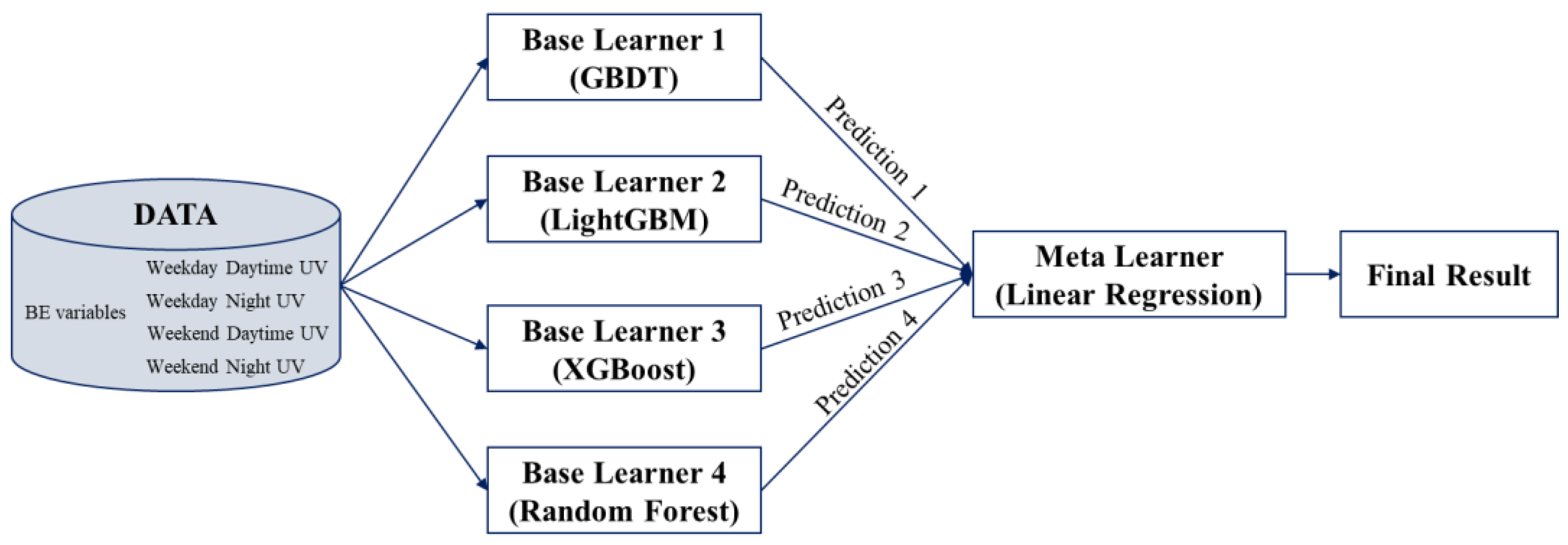
The framework of this study is illustrated in Figure 1. Firstly, multi-source data are obtained to measure the independent and dependent variables. The independent variables are screened by OLS models, and four well-performing base models are integrated using the ensemble machine learning algorithm, and are used to construct an analytical model of BE and UV. Finally, the SHAP algorithm is used to interpret the model and analyse the relative importance, nonlinear effect, threshold effect, interaction effect and local individual analysis of the impacts of BE on spatio-temporal heterogeneity of UV.

3.1. Study Area

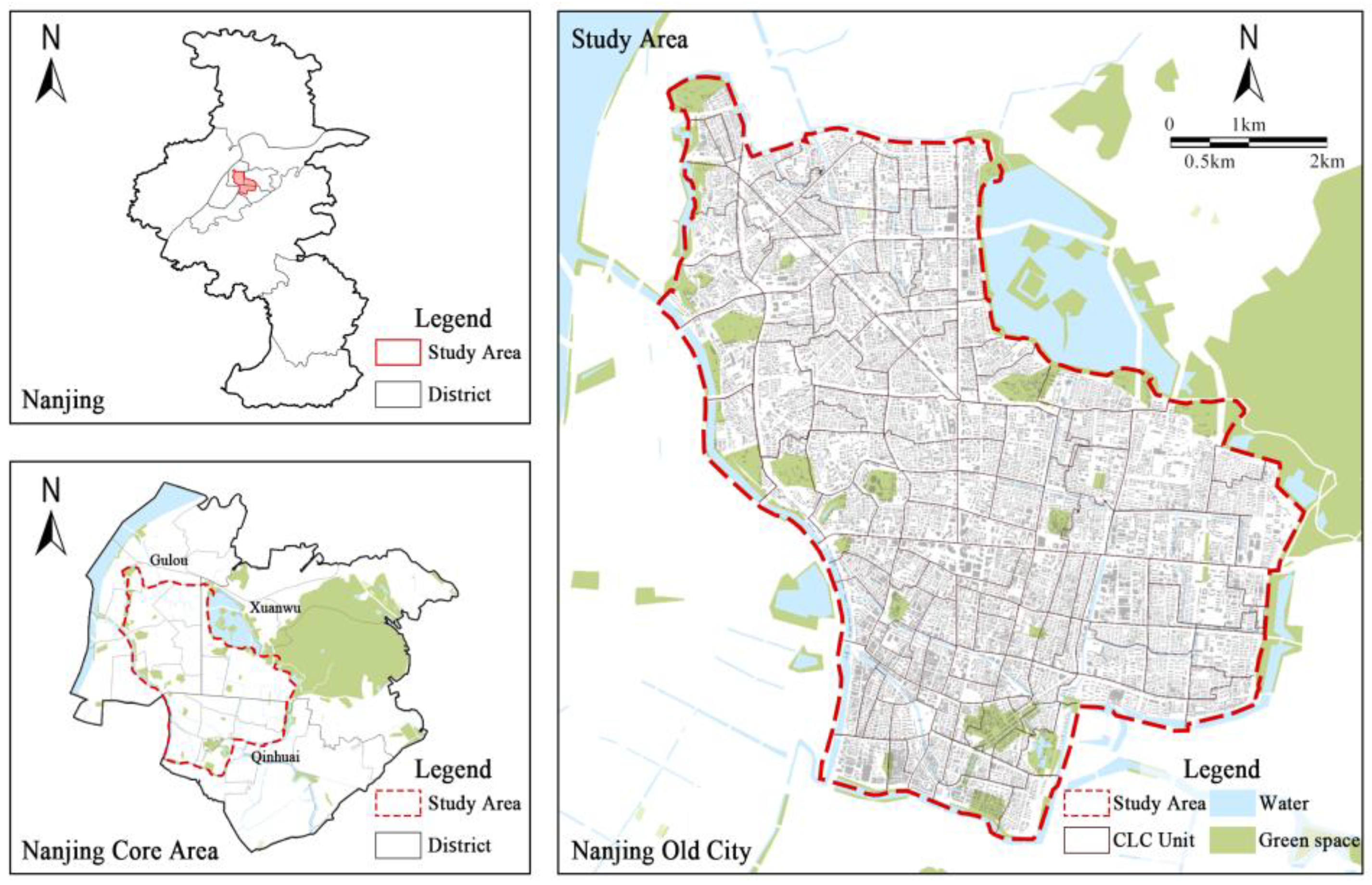
The research area selected for this study is the historic core of Nanjing, delineated by the ancient city walls, as shown in Figure 2. Nanjing is a central political, economic, cultural, and technological hub in eastern China. It holds significant strategic importance in the Yangtze River Economic Belt [35]. The designated study area, referred to as “Nanjing Old City,” is defined by the Ming Dynasty city wall as its primary boundary, covering an approximate area of 43 km². Compared to the areas beyond the city walls, the study area exhibits diverse and well-established urban spatial patterns, with stable and varied human activity dynamics, and the choice of this study area can effectively reduce the interference of urban location differences on the results of the study. However, the Old City also faces challenges such as functional decline, physical deterioration, and ecological degradation, which have hindered the full activation of UV. Therefore, this study selects 129 CLC units within the Nanjing Old City as the research objects (Figure 2). The CLC unit in this study is the unit of urban administration in China, and also the basic unit for the government to provide infrastructure and supporting living services.

3.2. Data Sources and Variable Description

3.2.1. Dependent Variables

The dependent variable in this study is the urban vitality of CLC units at different times of the week. The positioning database of Baidu Map Location-based Service (LBS) is used as the data source for our study. LBS data is actively located by mobile phone users through various location-related applications. It has high-precision spatial positioning and 24 h time stamps and is not affected by the density of signal base stations [36]. The total number of daily positioning requests within our study area exceeds one million, and the average precision of positioning points is as high as 20 m (https://lbsyun.baidu.com/products/location, accessed on 16 June 2025). Although it is difficult for LBS data to achieve full-time coverage of the entire population, especially for children and the elderly who rarely use mobile devices. However, the Baidu Map LBS database provides accurate and widely covered population travel data, and the travel records of most people can be generally recognized. If an ID repeatedly sends positioning requests in the same CLC unit within the same hour, its location will be recorded only once. The LBS data was cleaned through data deduplication and verification to improve the accuracy and overall quality of the data.

To explore the impact of the BE variables on UV in different time periods of the week, this study counted the frequency of LBS data within each CLC unit in a given week in 2025. The UV was further divided into four time periods: weekday daytime (average daily: 8 a.m.–16 p.m. from 16 to 20 June 2025), weekday nighttime (average daily: 16 p.m.–24 p.m. from 16 to 20 June 2025), weekend daytime (average daily: 8 a.m.–16 p.m. from 21 to 22 June 2025) and weekend nighttime (average daily: 16 p.m.–24 p.m. from 21 to 22 June 2025). It should be pointed out that Baidu Map LBS data is all anonymous, so personal privacy is strictly protected.

3.2.2. Independent Variables

The independent variable in this study is the BE variable at the CLC unit scale. As shown in

Table 1. Dependent variable descriptions.

Category	Metrics	Formula	Description
Function	Service POI density (SPOID)	$\mathrm{S}\mathrm{P}\mathrm{O}\mathrm{I}\mathrm{D}={\displaystyle \frac{{\mathrm{S}\mathrm{u}\mathrm{m}}_{\mathrm{S}\mathrm{i}}}{{\mathrm{A}}_{\mathrm{i}}}}$	Where ${\mathrm{S}}_{\mathrm{i}}$ is the total number of service POI in unit, and ${\mathrm{A}}_{\mathrm{i}}$ is the area of each unit.
	Office POI density (OPOID)	$\mathrm{O}\mathrm{P}\mathrm{O}\mathrm{I}\mathrm{D}={\displaystyle \frac{{\mathrm{S}\mathrm{u}\mathrm{m}}_{\mathrm{O}\mathrm{i}}}{{\mathrm{A}}_{\mathrm{i}}}}$	Where ${\mathrm{O}}_{\mathrm{i}}$ is the total number of production POI in unit, and ${\mathrm{A}}_{\mathrm{i}}$ is the area of each unit.
	Public POI density (PPOID)	$\mathrm{P}\mathrm{P}\mathrm{O}\mathrm{I}\mathrm{D}={\displaystyle \frac{{\mathrm{S}\mathrm{u}\mathrm{m}}_{\mathrm{P}\mathrm{i}}}{{\mathrm{A}}_{\mathrm{i}}}}$	${\displaystyle \frac{{\mathrm{S}\mathrm{u}\mathrm{m}}_{\mathrm{P}\mathrm{i}}}{\mathrm{A}}}$, Where ${\mathrm{P}}_{\mathrm{i}}$ is the total number of public POI in unit, and ${\mathrm{A}}_{\mathrm{i}}$ is the area of each unit.
	POI mixability (POIM)	$\mathrm{P}\mathrm{O}\mathrm{I}\mathrm{M}=-{\displaystyle \sum _{\mathrm{i}=1}^{\mathrm{n}}}{\mathrm{P}}_{\mathrm{i}}\log {\mathrm{P}}_{\mathrm{i}}$	Where ${\mathrm{P}}_{\mathrm{i}}$ is the percentage of POI types in a unit.
Morphology	Floor area ratio (FAR)	$\mathrm{F}\mathrm{A}\mathrm{R}={\displaystyle \frac{{\sum }_{\mathrm{i}=1}^{\mathrm{n}}{\mathrm{A}}_{\mathrm{T}\mathrm{i}}}{{\mathrm{A}}_{\mathrm{i}}}}$	Where ${\mathrm{A}}_{\mathrm{T}\mathrm{i}}$ is the total area of building in a unit, and ${\mathrm{A}}_{\mathrm{i}}$ is the area of each unit.
	Building density (BD)	$\mathrm{B}\mathrm{D}={\displaystyle \frac{{\sum }_{\mathrm{i}=1}^{\mathrm{n}}{\mathrm{A}}_{\mathrm{B}\mathrm{i}}}{{\mathrm{A}}_{\mathrm{i}}}}$	Where ${\mathrm{A}}_{\mathrm{B}\mathrm{i}}$ is the base area of building, $\mathrm{n}$ is the number of buildings in a unit, and ${\mathrm{A}}_{\mathrm{i}}$ is the area of each unit.
	Average building height (ABH)	$\mathrm{A}\mathrm{B}\mathrm{H}={\displaystyle \frac{{\sum }_{\mathrm{i}=1}^{\mathrm{n}}{\mathrm{H}}_{\mathrm{i}}}{\mathrm{n}}}$	Where ${\mathrm{H}}_{\mathrm{i}}$ is the building height, $\mathrm{n}$ is the number of buildings in a unit.
	Maximum building height (MBH)	$\mathrm{M}\mathrm{B}\mathrm{H}={\mathrm{H}}_{\mathrm{m}\mathrm{a}\mathrm{x}}$	Where ${\mathrm{H}}_{\mathrm{m}\mathrm{a}\mathrm{x}}$ is the height of the tallest building in a unit.
	Average building area (ABA)	$\mathrm{A}\mathrm{B}\mathrm{A}={\displaystyle \frac{{\sum }_{\mathrm{i}=1}^{\mathrm{n}}{\mathrm{A}}_{\mathrm{D}\mathrm{i}}}{\mathrm{n}}}$	Where ${\mathrm{A}}_{\mathrm{D}\mathrm{i}}$ is the Maximum building area in a unit, and $\mathrm{n}$ is the number of buildings in a unit.
	Maximum building area (MBA)	$\mathrm{M}\mathrm{B}\mathrm{A}={\mathrm{A}}_{\mathrm{m}\mathrm{a}\mathrm{x}}$	Where ${\mathrm{A}}_{\mathrm{m}\mathrm{a}\mathrm{x}}$ is the Maximum building area in a unit.
Transportation	Road density (RD)	$\mathrm{R}\mathrm{D}={\displaystyle \frac{{\sum }_{\mathrm{i}=1}^{\mathrm{n}}{\mathrm{S}}_{\mathrm{R}\mathrm{i}}}{{\mathrm{A}}_{\mathrm{i}}}}$	Where ${\mathrm{S}}_{\mathrm{R}\mathrm{i}}$ is the total length of the roads in a unit, and ${\mathrm{A}}_{\mathrm{i}}$ is the area of each unit.
	Intersection density (ID)	$\mathrm{I}\mathrm{D}={\displaystyle \frac{{\mathrm{S}\mathrm{u}\mathrm{m}}_{{\mathrm{I}}_{\mathrm{i}}}}{{\mathrm{A}}_{\mathrm{i}}}}$	Where ${\mathrm{I}}_{\mathrm{i}}$ is the total number of road intersections in a unit, and ${\mathrm{A}}_{\mathrm{i}}$ is the area of each unit.
	Bus stop density (BSD)	$\mathrm{B}\mathrm{S}\mathrm{D}={\displaystyle \frac{{\mathrm{S}\mathrm{u}\mathrm{m}}_{{\mathrm{C}}_{\mathrm{i}}}}{{\mathrm{A}}_{\mathrm{i}}}}$	Where ${\mathrm{C}}_{\mathrm{i}}$ is the total number of bus stops in a unit, and ${\mathrm{A}}_{\mathrm{i}}$ is the area of each unit.
	Metro station accessibility (MSA)	$\mathrm{M}\mathrm{S}\mathrm{A}={\displaystyle \frac{1}{{\mathrm{D}}_{\mathrm{m}\mathrm{i}\mathrm{n}}}}$	Where ${\mathrm{D}}_{\mathrm{m}\mathrm{i}\mathrm{n}}$ is the distance of the centre of gravity of the unit from the nearest metro station.
Ecology	Fractional vegetation cover (FCV)	$\mathrm{F}\mathrm{C}\mathrm{V}={\displaystyle \frac{{\mathrm{A}}_{\mathrm{v}}}{{\mathrm{A}}_{\mathrm{i}}}}$	Where ${\mathrm{A}}_{\mathrm{v}}$ represents the area of vegetation coverage and ${\mathrm{A}}_{\mathrm{i}}$ is the area of each unit.
	Normalized Difference Vegetation Index (NDVI)	$\mathrm{N}\mathrm{D}\mathrm{V}\mathrm{I}={\displaystyle \frac{\mathrm{N}\mathrm{I}\mathrm{R}-\mathrm{R}\mathrm{E}\mathrm{D}}{\mathrm{N}\mathrm{I}\mathrm{R}+\mathrm{R}\mathrm{E}\mathrm{D}}}$	Where $\mathrm{N}\mathrm{I}\mathrm{R}$ is the reflection value in the near-infrared band and $\mathrm{R}\mathrm{E}\mathrm{D}$ is the reflection value in the red band.
	Remote sensing ecological index (RESI)	$\mathrm{R}\mathrm{E}\mathrm{S}\mathrm{I}=\mathrm{P}\mathrm{A}\mathrm{C}(\mathrm{n}\mathrm{d}\mathrm{v}\mathrm{i},\mathrm{w}\mathrm{e}\mathrm{t},$$\mathrm{l}\mathrm{s}\mathrm{t},\mathrm{n}\mathrm{d}\mathrm{b}\mathrm{s}\mathrm{i})$	Where $\mathrm{n}\mathrm{d}\mathrm{v}\mathrm{i}$ is the normalized difference vegetation index, $\mathrm{w}\mathrm{e}\mathrm{t}$ is the relative humidity, $\mathrm{l}\mathrm{s}\mathrm{t}$ is the Land surface temperature, and $\mathrm{n}\mathrm{d}\mathrm{b}\mathrm{s}$ is the normalized difference built-up and soil index.

, a bottom-up metric system is built to quantify the BE from four categories: function, morphology, transportation, and ecology. The data for the function dimension indicators are from the Gaode Map Open Platform (https://lbs.amap.com, accessed on 16 June 2025). Since the POI data is too redundant, we deleted some points with low public recognition, and classified all POIs into three categories: service, production, and public. Finally, the density index and the mixing degree of the three types of POIs are calculated. The morphology and traffic dimension indicator data are taken from vector maps in Bigemap Gis Office (http://www.bigemap.com, accessed on 16 June 2025), which can be downloaded to perform calculations in ArcGis 10.7 according to the formulae in Table 1. Data for the Ecology dimension indicators were obtained from the National Ecological Data Centre of the Chinese Academy of Sciences (https://nesdc.org.cn/, accessed on 16 June 2025). In the ENVI 5.3 platform, four types of data, NDVI, WET, NDBISI, and LST, could be calculated, and the four indices were standardized using the normalization tool. Then, the four indices were synthesized into one dataset in the order of NDVI, WET, NDBISI, and LST through the Layer stacking tool, and the principal component analysis was carried out using the Transform > PCARotation > Forward PCA Rotation New Statistics and Rotate tool in ENVI to obtain the RSEI index results of each CLC unit in the research area. The specific calculation formulas of each variable are shown in Table 1. In order to verify the effectiveness of be index classification structure, this study uses Cronbach’s alpha to test, and the four dimensions of Cronbach’s alpha are 0.915, 0.867, 0.732 and 0.856, respectively, indicating the effectiveness of the index system.

3.3. Ordinary Least Squares (OLS) Model

By synthesizing the main BE factors affecting UV in existing studies and combining with the characteristics of the Nanjing Old City, 17 potential factors were determined for analysis. It is necessary to conduct a multicollinearity analysis on these variables. The OLS model is a global regression technique used to ascertain the relationship between dependent variables and various independent variables [37]. The model results may be distorted since there may be a strong correlation between some BE variables. The basic principle of the OLS method is to regard each variable as the dependent variable, in turn, through linear regression analysis, while other variables are considered independent variables. The higher the coefficient of determination, the higher the probability of multicollinearity between the variable and other variables. The OLS method was used to analyze the multicollinearity of all potential BE factors affecting UV. The factors that did not meet the requirements of standard deviation and VIF were removed, and the input types of the final BE factors were determined. IBM SPSS Statistics 25 was used for linear regression analysis, and linear selection, multicollinearity, and variable selection were incorporated into the OLS model. The OLS model can be expressed using Equation (1):

$${\mathrm{y}}_{\mathrm{i}}={\mathrm{A}}_0+\sum _{\mathrm{i}}^{\mathrm{n}}{\mathrm{A}}_{\mathrm{i}}{\mathrm{x}}_{\mathrm{i}}+{\mathsf{\lambda }}_{\mathrm{i}}$$

(1)

where ${\mathrm{y}}_{\mathrm{i}}$ represents the dependent variable; ${\mathrm{A}}_0$ represents the intercept; ${\mathrm{x}}_{\mathrm{i}}$ represents the independent variable; ${\mathrm{A}}_{\mathrm{i}}$ represents the regression coefficient; $\mathrm{n}$ represents the number of independent variables; ${\mathsf{\lambda }}_{\mathrm{i}}$ represents a random error term.

3.4. Ensemble Machine Learning

Ensemble machine learning is a class of strategies for improving the generalization ability of machine learning models. It makes up for the deficiencies of a single learner through the combination of multiple learners. Since various machine learning algorithms have different characteristics, they will show different performances in the urban vitality modeling tasks at different time periods. Therefore, obtaining the optimal results through a single machine learning algorithm is difficult. Ensemble machine learning balances Bias and Variance by integrating multiple base learners to reduce the Generalization Error of the model, thereby constructing a more robust final model suitable for different time periods. Ensemble learning mainly includes three categories: bagging, boosting, and stacking [38]. The bagging approach trains multiple independent models through bootstrap sampling to reduce variance. The Boosting approach can reduce the bias by iteratively training the weak learner to focus on the samples that are difficult to classify. In contrast, the stacking approach combines multiple outstanding base learners. It uses a meta learner to implement an optimal combination strategy for the prediction results of base learners, reducing both bias and variance at the same time, to integrate the advantages of different models and improve the generalization performance of the model. In this study, the Stacking strategy was used for ensemble learning. The specific process is as follows:

• This study uses 8 standard machine learning algorithms to model BE and UV data in four time periods. Moreover, the regression coefficient of determination (R²) was used as the evaluation index to comprehensively compare the prediction performances of each algorithm under different time periods (

  Table 2. Prediction Accuracy of Different Machine Learning Simulation Models.

  Model	R2 (Coefficient of Determination)
  	Weekday Daytime	Weekday Nighttime	Weekend Daytime	Weekend Nighttime
  GBDT	0.8423	0.6749	0.7649	0.6242
  LightGBM	0.8220	0.7390	0.7945	0.6459
  XGBoost	0.7976	0.6219	0.7438	0.6776
  Random Forest	0.7862	0.7779	0.7955	0.7167
  K-Nearest Neighbors	0.7343	0.5640	0.5808	0.5293
  Decision Tree	0.6350	0.5662	0.4842	0.1706
  Ridge Regression	0.2077	0.6597	0.2516	0.5970
  Linear Regression	0.1791	0.6775	0.2649	0.6199
  Stacking (Select GBDT, LightGBM, XGBoost and Random Forest)	0.8039	0.7567	0.7816	0.6730

  The bold-faced fonts represent the top 4 models with the highest R² performance in each time period.

  ).

2.

Four algorithms (GBDT, LightGBM, XGBoost, and Random Forest) with stable performance and high R² in all time periods were comprehensively considered as the final base learners. It should be noted that although XGBoost was not one of the top four algorithms in the “weekday evening” time period, since it always performed excellently in other time periods, to ensure the consistency of the model structure between different time periods and reduce the external interference caused by algorithm differences, it was still included in the unified modeling system.

3.

To further improve the performance of each base model, the Bayesian Optimization method was used to automatically tune its key hyperparameters to ensure that it participated in the ensemble modeling under the optimal parameter configuration.

4.

In the Stacking strategy, Linear Regression was selected as the meta learner to remodel the prediction results of the four base learners. Logistic Regression can effectively learn the optimal weights of each base learner in the final prediction and implement a weighted combination of the results, thereby integrating each model’s advantages and improving the ensemble model’s robustness. The algorithm principle of ensemble machine learning is shown in Figure 3.

3.5. SHAP Algorithm

SHAP (Shapley Additive Explanations) is an additive feature attribution algorithm grounded in cooperative game theory, designed to quantify the marginal contribution of each independent variable to model predictions, providing interpretability to machine learning models [39]. This approach calculates SHAP values by decomposing model predictions into a baseline value and the linear sum of all feature contributions. By doing so, SHAP simultaneously evaluates local (individual sample), global (whole dataset), and interaction effects, significantly enhancing the transparency of machine learning models. As a result, it has been widely applied in interpretable machine learning [40]. For any given prediction sample, the SHAP value represents the contribution of each feature to the model output relative to the baseline value, and its mathematical expression is Equation (2):

$${\mathsf{\varphi }}_{\mathrm{i}}=\sum _{\mathrm{S}\subseteq \mathrm{N}\left\{\left.\mathrm{i}\right\}\right.}{\displaystyle \frac{\left|\mathrm{S}\right|!(\mathrm{M}-\left|\mathrm{S}\right|-1)!}{\mathrm{M}!}}\left[\mathrm{v}\left(\mathrm{S}\cup \left\{\left.\mathrm{i}\right\}\right.\right)-\mathrm{v}\left(\mathrm{S}\right)\right]$$

(2)

where ${\mathsf{\varphi }}_{\mathrm{i}}$ represents the contribution of the feature $\mathrm{i}$, $\mathrm{N}\left\{\left.1,2..\mathrm{M}\right\}\right.$ represents the subscript of the feature variable in the dataset, $\mathrm{M}$ is the total number of feature variables. $\mathrm{S}$ is a subset of the set $\left\{\left.\mathrm{1,2}..\mathrm{i}-1,\mathrm{i}+1,..\mathrm{M}\right\}\right.$, $\left|\mathrm{S}\right|$ is the total number of elements in $\mathrm{S}$. $\mathrm{v}\left(\mathrm{S}\cup \left\{\left.\mathrm{i}\right\}\right.\right)$ represents the predicted value of the model when only the features in $\mathrm{S}\cup \left\{\left.\mathrm{i}\right\}\right.$ are present, while $\mathrm{v}\left(\mathrm{S}\right)$ represents the predicted value of the model when only the features in $\mathrm{S}$ are present, and the difference between the two is the marginal contribution of the $\mathrm{i}$th feature variable under the subset $\mathrm{S}$.

Then, the SHAP values were computed using an additive feature attribution method, and its mathematical expression is Equation (3):

$$\mathrm{g}\left(\mathrm{z}\right)={\mathrm{\varnothing }}_0+\sum _{\mathrm{i}=1}^{\mathrm{M}}{\mathrm{\varnothing }}_{\mathrm{i}}{\mathrm{z}}_{\mathrm{i}}$$

(3)

where $\mathrm{g}\left(\mathrm{z}\right)$ represents the predicted value influenced by the feature variables, ${\mathrm{\varnothing }}_0$ is a constant indicating the expected value of the model prediction. $\mathrm{M}$ is the number of features, $\mathrm{z}$ indicates the presence of corresponding features, ${\mathrm{\varnothing }}_{\mathrm{i}}$ is the coefficient in the explanation model, it represents the attribution of the $\mathrm{i}$th feature to the model prediction. Since this study uses an ensemble learning model, we applied the Kernel Explainer in SHAP package (Python 3.9) to calculate both SHAP values and SHAP interaction values.

4. Results

4.1. The Spatial and Temporal Differentiation of Urban Vitality

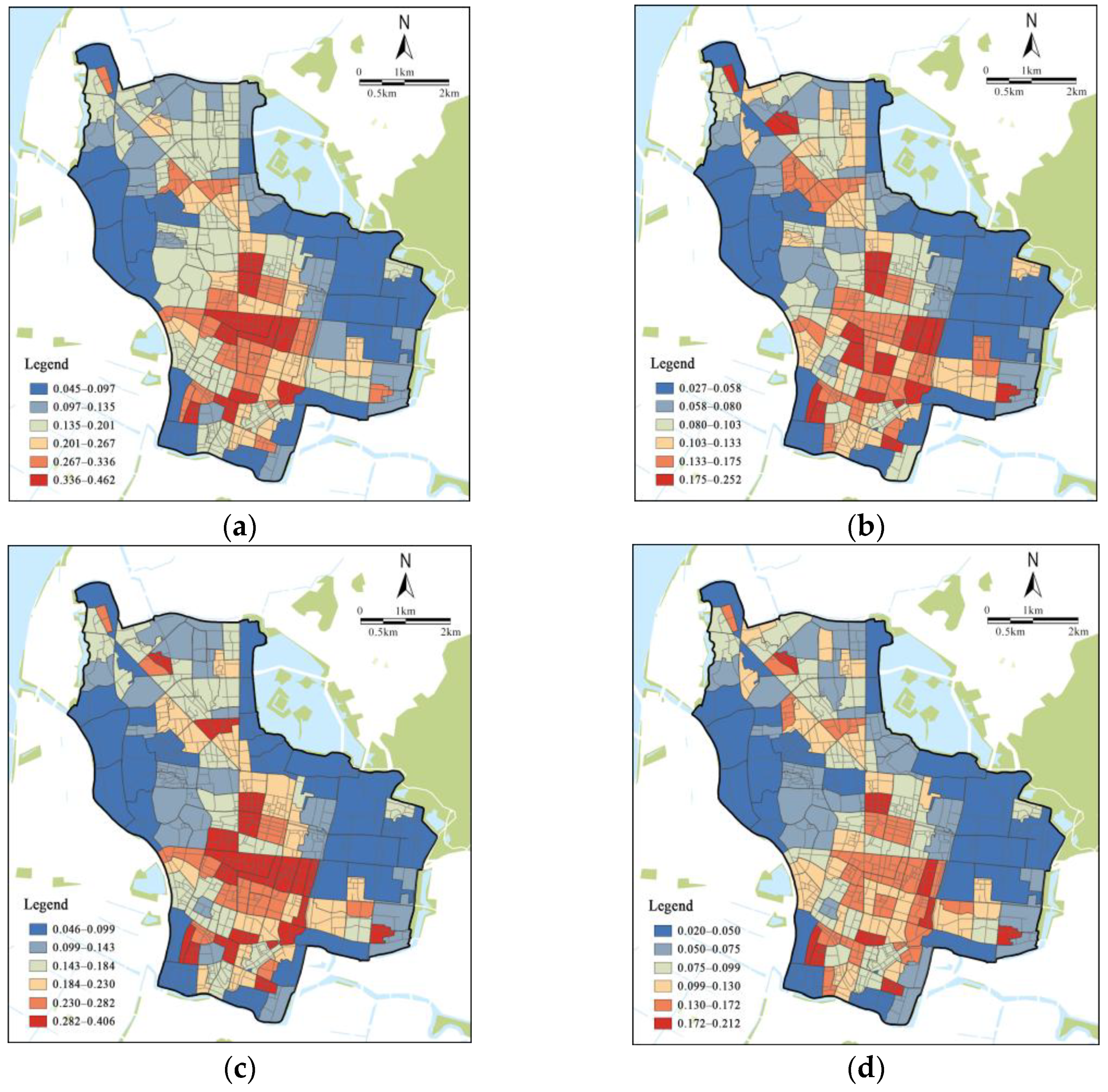
Figure 4 illustrates the distribution and intensity of UV across different time periods. The UV value is higher overall during the day than at night, and slightly higher on weekdays than on weekends. The fact that the UV of a large number of CLC units on weekends was concentrated at a low or relatively low level suggests a lack of incentive for urban residents to go out at weekends. There are a few CLC units with high UV at night on weekends, which indicates that the UV of the Nanjing Old City has declined to a certain extent.

Figure 5 presents the spatio-temporal distribution of UV across different time periods. Overall, the results indicate a pronounced clustering effect and an uneven spatial distribution of UV in the study area. Higher UV value units are predominantly located in the central areas and along major urban corridors. In contrast, units near the eastern and western edges of the city wall generally exhibit lower UV, with more pronounced day-night fluctuations. Figure 5a demonstrates that on weekdays during the daytime, higher UV is concentrated in several business centers along the city’s main corridors. Figure 5b shows that some CLC units in the central business district experience vitality depressions at night, indicating that specific communities fail to sustain high activity levels. Figure 5c,d reveal that on weekends, relatively higher UV units emerge on the outskirts of business districts, suggesting that many residents tend to engage in leisure and recreational activities near their residential areas [41].

4.2. Linear Regression Results of Influencing Factors of UV Based on OLS Model

Considering that multicollinearity will significantly affect the effectiveness of machine learning models, the OLS model was adopted to evaluate the relationship between two or more BE variables. The results of multicollinearity diagnosis during weekday daytime are shown in

Table 3. Multicollinearity diagnosis results of weekday daytime. (The full names of metrics can be referenced in Table 1).

Metrics	Coefficient	Std	Tolerance	VIF
SPOID	5.266	0.034	0.190	5.266
OPOID	4.712	0.116	0.212	4.712
PPOID	3.316	0.001	0.319	3.136
POIM	2.493	0.002	0.401	2.492
FAR	0.538	0.008	0.109	8.055
BD	−0.032	0.012	0.160	6.241
ABH	3.076	0.001	0.325	3.076
MBH	2.111	0.001	0.474	2.111
ABA	1.660	0.001	0.602	1.660
MBA	1.464	0.001	0.683	1.464
RD	1.335	0.039	0.749	1.335
ID	1.428	0.043	0.093	10.728
BSD	2.789	0.003	0.359	2.789
MSA	1.237	0.001	0.808	1.237
FCV	10.728	0.009	0.136	9.347
NDVI	10.356	0.011	0.086	11.583
RESI	11.583	0.013	0.253	8.427

, the Tolerance and VIF are consistent for the rest of the time period. The results indicated that the tolerance values of almost all BE variables exceeded 0.1. Except for intersection density (ID) and normalized difference vegetation index (NDVI), the VIF values were all less than 10. The tolerance values of ID and NDVI were 0.093 and 0.086, respectively. Their VIF values were 10.728 and 11.583, respectively, both exceeding 10. The main reason for this phenomenon was that the ID data was greatly affected by the road network density data, and the NDVI data was derived from the FCV data. Therefore, the ID and NDVI indicators were removed, and the other 15 BE variables were retained to explore their influencing effects on urban vitality. Meanwhile, the tolerance and VIF values of the remaining 15 BE indicators all met the requirements. Thus, it was considered that the factor detection system constructed by 15 BE factors met the requirements of the OLS model.

4.3. Relative Importance of BE Variables

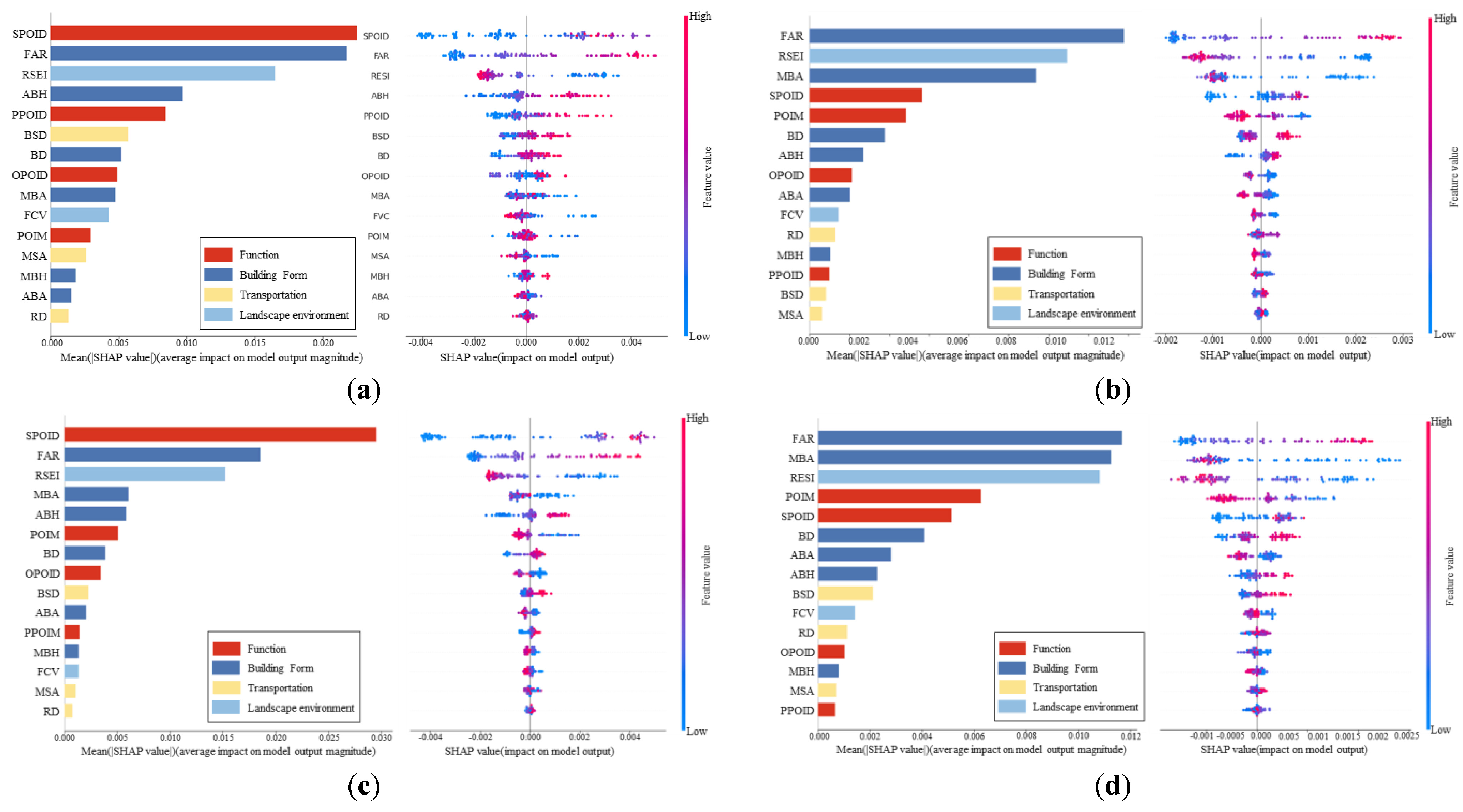
The SHAP algorithm is used to interpret the contribution of independent variables in machine learning models to the prediction results. The sum of the relative importance values of all independent variables equals 1, accurately reflecting the impact of each BE variable on UV across different time periods. The bar chart in Figure 6 arranges BE variables in descending order based on their global correlation, with the mean SHAP value on the horizontal axis representing their relative importance. SPOID, FAR, and RESI consistently maintain high importance across all time periods, indicating that they are the primary determinants of UV’s spatial distribution. Meanwhile, results suggest that the impact of transportation dimension on urban vitality is not significant in different time periods. On the one hand, it shows that the total length of roads per unit area has a weak impact on UV. On the other hand, it shows that due to the small regional differences in the study area, and the overall convenience of public transport [42].

4.4. Nonlinear and Threshold Effects of Built Environment Variables

This study employs SHAP-based local dependence plots (LDPs) to reveal the effects of BE factors on UV across different time periods of the week. The fitted curves in the plots smooth the scatter points, where steeper slopes indicate higher marginal effects of the independent variables. This method enables a direct and in-depth understanding of the commonalities and differences in how BE factors influence UV at different time periods, allowing for the quantification of variable threshold points. It is noteworthy that, given the large number of BE variables, this study selects the top 7 most important BE variables in each time period for analysis. Figure 7 illustrates the nonlinear effects and threshold effects of BE variables on UV.

The BE variables in the functional dimension have obvious threshold effects and marginal effects on the UV in the study area. Figure 7a,n,p,z show that SPOID is positively correlated with UV across all time periods, with thresholds of 4 during the daytime and 3 at night, but the marginal effect of this positive influence diminishes, which is consistent with most previous research [43]. Figure 7e shows that PPOID has a significant positive effect on UV only during weekdays in the daytime, with a threshold of 0.9. Figure 7k,t,y illustrate that POIM exhibits a pronounced effect on UV during all time periods except for weekday daytime, demonstrating a segmented influence pattern with a threshold of 1.8. When the POIM ranges between 1.4 and 1.8, it has a stable positive effect. However, once this threshold is exceeded, its effect rapidly shifts to negative, which is particularly evident at night. This result suggests that excessive functional diversity may lead to a decline in UV.

There are positive or negative impacts between different BE variables in the morphological dimension and UV, and the threshold effects vary in different time periods. Figure 7b,h,o,x show that FAR exhibits a similar nonlinear relationship with UV across all time periods, with thresholds of 1.5 during the daytime and 1.4 at night. When the FAR exceeds approximately 2.0, its marginal effect on UV gradually diminishes. This result suggests that excessively high FAR may create spatial oppression, thereby restricting the growth of UV [18]. Figure 7d,l,β indicate that ABH shows a positive correlation with UV across all time periods, with a threshold of 11.5, but its marginal effect sharply declines beyond 15. Figure 7u,i,s,w illustrate that ABA and MBA exhibit positive effects on UV when the ABA is below 200 and the MBA is below 3000.

The importance of the transportation dimension’s BE variables on the UV of the study area is relatively low, due to the high coverage of transport facilities in CLC units within the Nanjing Old City. BSD exhibits distinct nonlinear effects on UV during weekday daytime and nighttime (Figure 7g,m). During the daytime, the threshold value is 0.15, and when BSD ranges between 0.15 and 0.25, it has a positive effect on UV. At nighttime, BSD maintains a positive effect within the range of 0.13 to 0.28, but beyond 0.28, its contribution to vitality growth gradually diminishes.

The BE variables of the ecological dimension have significant impacts on UV across time. RESI demonstrates a consistent nonlinear relationship with UV across all time periods, with threshold values of 0.39 during daytime and 0.41 at night (Figure 7c,j,q,v). The results indicate that when RESI is less than 0.35, it has a stable positive effect on UV throughout the day. However, when RESI surpasses 0.45, it hinders spatial activity clustering and negatively impacts UV. Similarly, FCV exhibits a declining positive effect on UV within the range of 0.1 to 0.32, reaching its peak influence around 0.3, but turning negative beyond 0.32.

4.5. Interaction Effects of Key Built Environment Variables

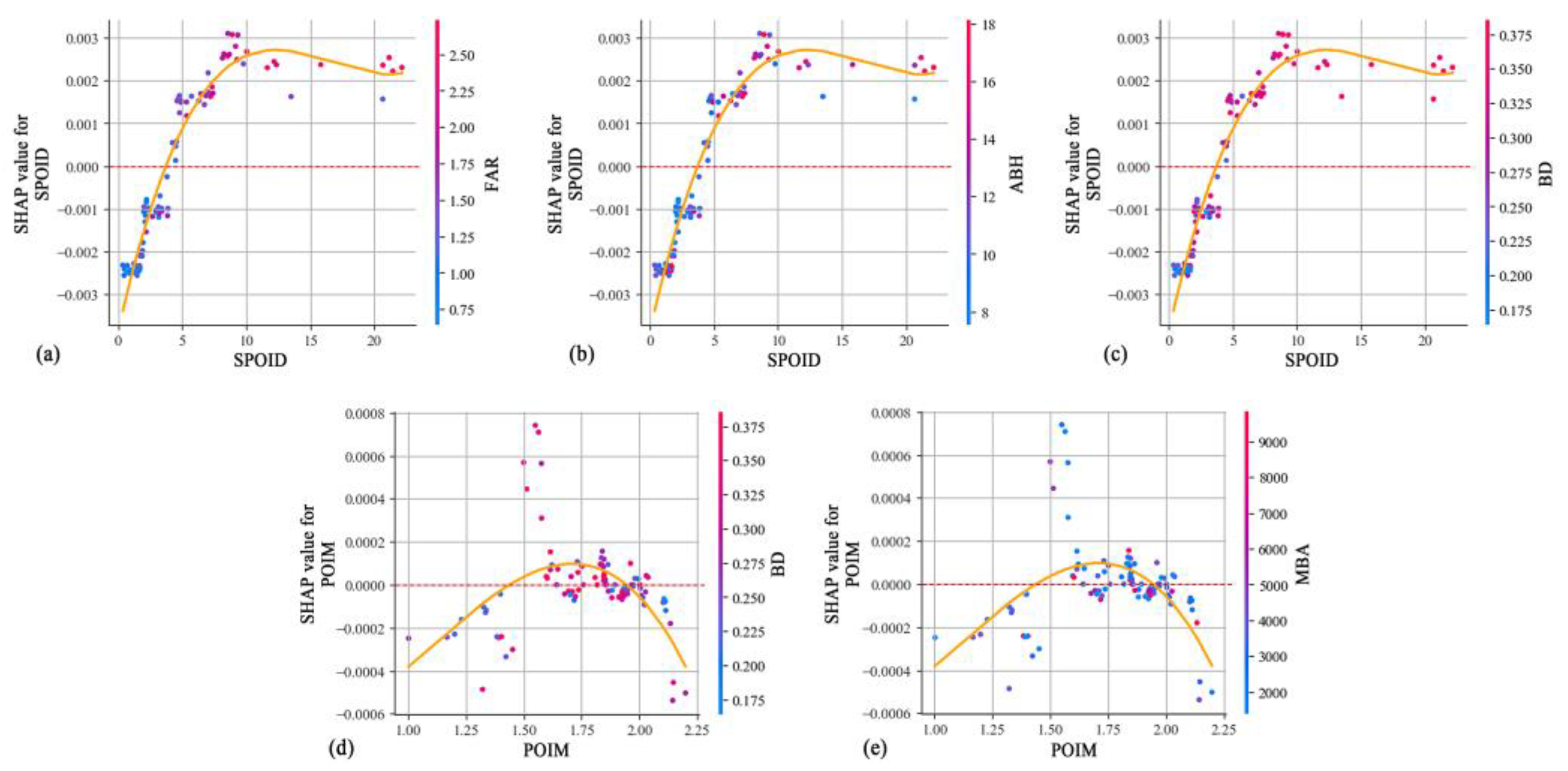
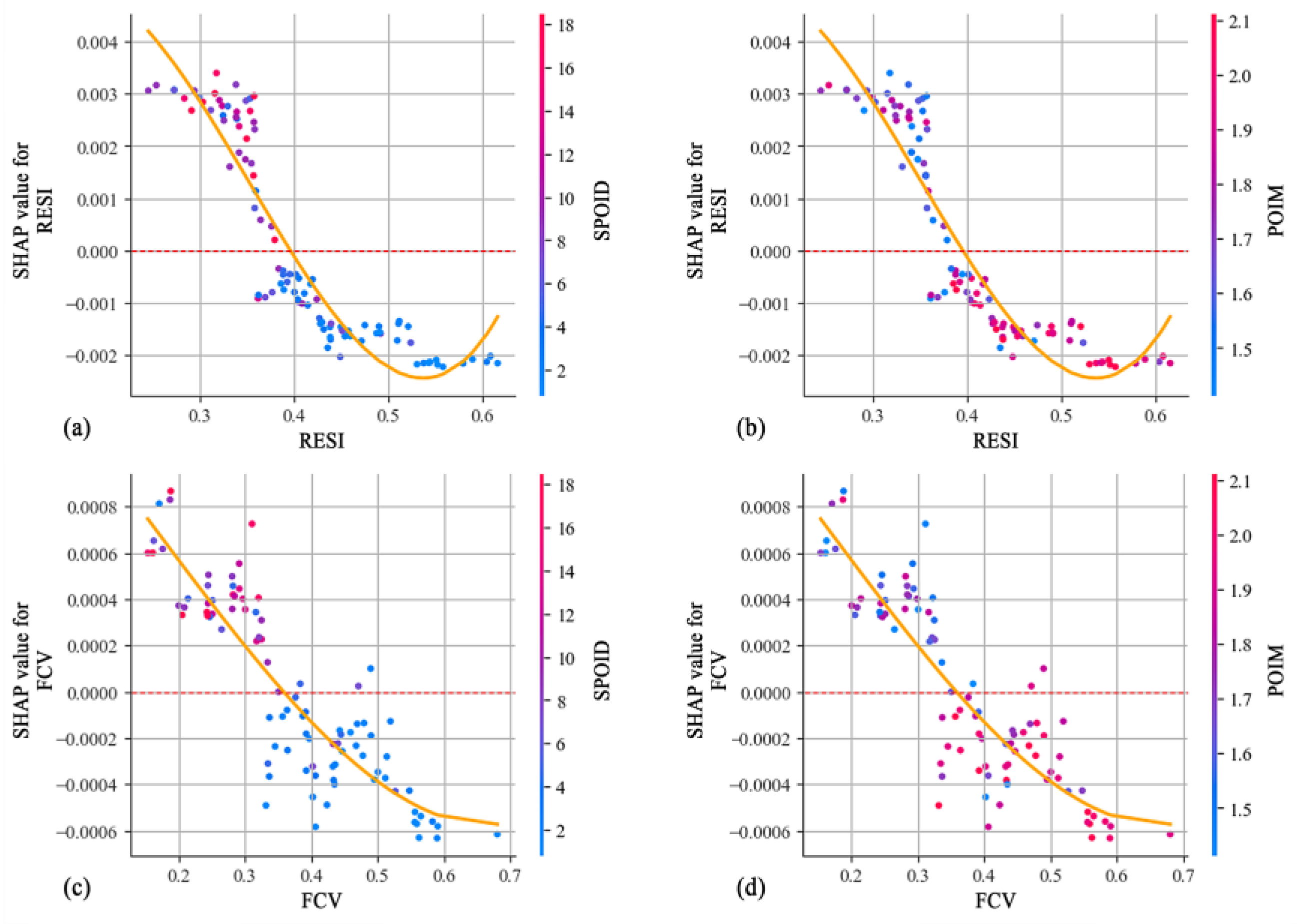
Through the SHAP algorithm, the local effects of explanatory variables (SHAP values) are decomposed into main local effects and local interaction effects with other variables [44]. This study selects the eight most important variables across three dimensions (function, morphology, ecology) and examines their interaction effects during weekday daytime as an example (Figure 8, Figure 9 and Figure 10). Each figure visualizes the interaction between two variables, where each point represents a CLC unit. The X-axis indicates one independent variable, the color represents the magnitude of the interacting variable, and the Y-axis shows the SHAP interaction effect values between the two variables.

4.5.1. Interaction Effects Between Function and Morphology Dimensions

Figure 8a–c demonstrate strong interaction effects between SPOID and FAR, ABH, BD. When SPOID > 5 and FAR > 1.75, ABH > 14, BD > 0.325, a significant positive interaction effect emerges. However, when SPOID > 5, some units with lower ABH still maintain high UV value. A possible explanation is that urban service functions, which attract urban vitality, and are often suitable for lower floors of buildings [45]. When BD remains high, further increasing SPOID does not necessarily improve UV and may even lead to a decline. This could be due to the over-homogenization of urban functions, where excessive uniformity in service offerings reduces attractiveness. Figure 8d,e illustrate that when POIM is between 1.5 and 1.75, BD > 3, and MBA < 3000, strong local interaction effects are observed. A balanced POIM is essential for UV, as an excessively high POIM may result in inefficient land use and diminished UV. Urban planners should strategically allocate urban functions based on building morphology, optimizing the balance between service types to attract foot traffic and stimulate economic activity.

4.5.2. Interaction Effects Between Morphology and Ecology Dimensions

Figure 9a,b reveal that when FAR is between 1.5 and 2.5, RESI is between 0.30 and 0.40, and FCV is between 0.2 and 0.3, their positive interaction effect is most pronounced. Beyond this range, further increasing FAR does not improve UV, likely because excessively high FAR contributes to traffic congestion and infrastructure strain, thereby diminishing residents’ spatial experiences. This result underscores the need to prevent overdevelopment and maintain a livable community environment. Figure 9c,d show that when BD is 0.25, RESI is between 0.40 and 0.50, and FCV is between 0.35 and 0.45, the positive interaction effect reaches its peak. When BD is between 0.25 and 0.30, and RESI and FCV are high, they exhibit synergistic effects on UV. One explanation is that some CLC units with eco-orientated development are able to create high vitality while maintaining low development intensity [46]. Figure 9e illustrates that the interaction effect on UV is strongest when ABH is between 12 and 17 and FCV is between 0.3 and 0.35. Excessively high or low ABH negatively impacts UV. Figure 9f demonstrates that when MBA < 3000 and RESI is between 0.30 and 0.45, the positive interaction effect is strongest. Furthermore, an interaction effect on UV is still observed when MBA is between 10,000 and 17,000, and RESI is between 0.40 and 0.50. These findings suggest that urban planners should implement differentiated planning strategies to meet the varied demands of residents for building space and an ecological environment.

4.5.3. Interaction Effects Between Ecology and Function Dimensions

Significant interaction effects exist between the ecology and functional dimensions. Figure 10a shows that when RESI is between 0.25 and 0.35, and SPOID is within the high range of 8 to 18, the two variables exhibit a strong positive interaction effect. Conversely, Figure 10b indicates that a positive interaction effect is also observed when RESI is between 0.25 and 0.35, and POIM is in the lower range of 1.5 to 1.8. The interaction effect of FCV with functional dimensions is similar to that of RESI. Figure 10c illustrates that when FCV is between 0.2 and 0.3, SPOID is between 10 and 18, POIM is between 1.5 and 1.8, they exhibit a positive interaction effect. As FCV increases, reducing SPOID leads to a decline in UV, whereas an increase in POIM also results in vitality loss. These findings suggest that a well-developed ecological environment amplifies the positive impact of commercial service functions on UV. The threshold of POIM should also be controlled to ensure that the mix of functions is appropriate and coordinated [47].

4.6. Clustering Results and SHAP Local Explanations

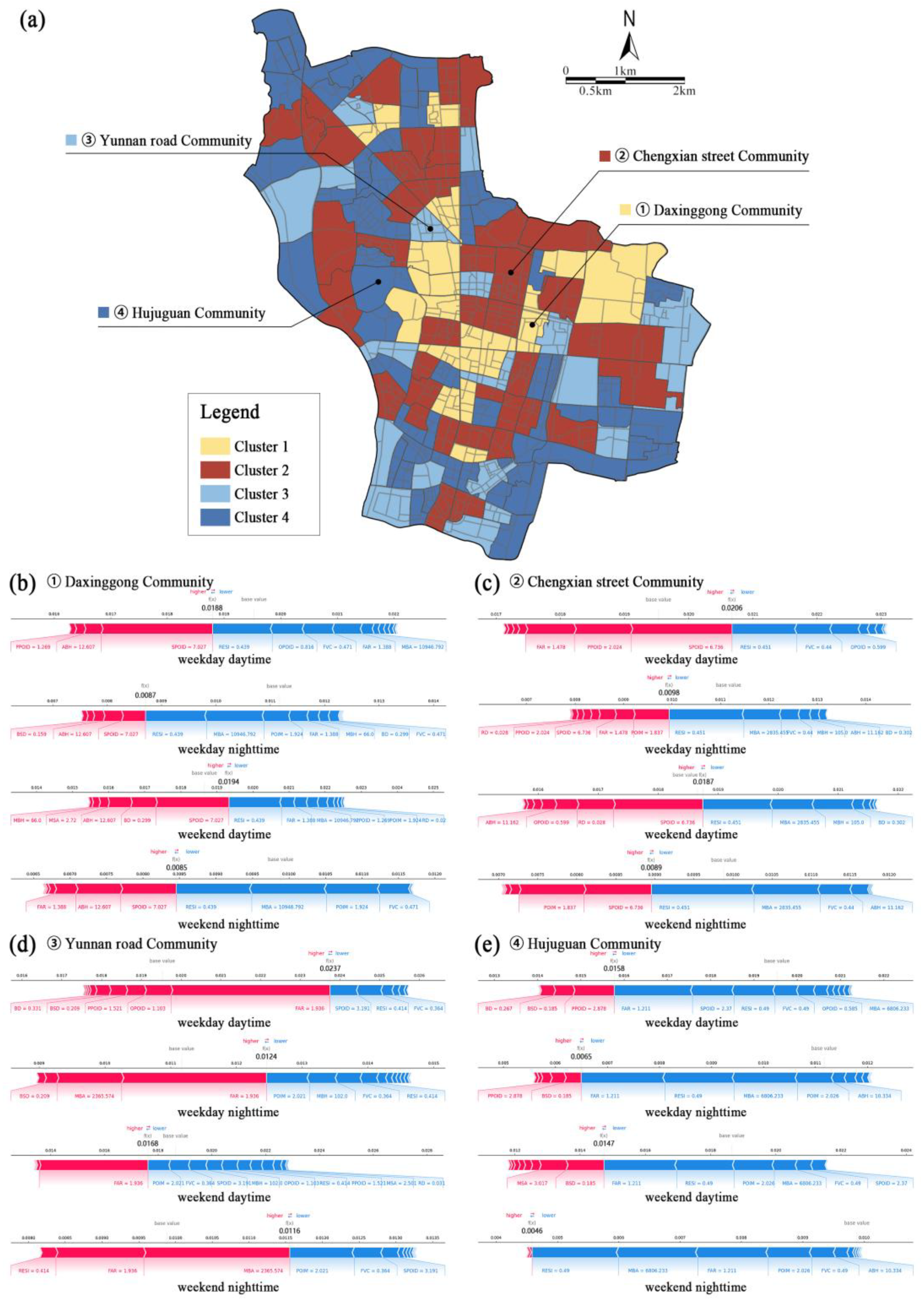
This study applies the SHAP algorithm to interpret individual unit characteristics to reveal the spatio-temporal heterogeneity of BE impacts on UV and provide tailored planning recommendations for different CLC units [48]. Each unit’s SHAP values across all BE variables are compiled into a vector, which is then clustered using hierarchical clustering to identify unit types with similar local effects [49]. Figure 11a visualizes the spatial distribution of the four generated clusters. The four clusters account for 11.6%, 32.6%, 40.3%, and 15.5%, respectively. This study selects representative CLC units from each cluster for further analysis.

The case in Cluster 1 includes significant urban commercial and cultural functions, such as the Presidential Palace and Nanjing Library (Figure 11b). In the Daxinggong Community, commercial service functions consistently play the most critical role in improving UV across all time periods, with SHAP values exceeding 7. However, the impact of morphology indicators varies significantly across different time periods, suggesting that people prefer different spatial environments depending on the time of week. Consequently, urban planning and design should provide diverse architectural experiences tailored to different time periods.

The case in Cluster 2 comprises Southeast University and its surrounding residential functions (Figure 11c). In the Chengxian Street Community, functional indicators play a significant role in enhancing urban vitality. For university communities and adjacent residential areas, convenient and diverse urban functions are essential across all time periods. Additionally, urban vitality is further enhanced when FAR reaches 1.478 and ABH is 11.461. A possible explanation is that residents in educational districts tend to prefer low-rise residential environments that offer a stronger sense of community and daily life engagement.

The case in Cluster 3 includes landmark high-rise buildings such as Zifeng Tower (Figure 11d). The Yunnan Road Community benefits from the attraction of these iconic skyscrapers, which significantly contribute to UV. However, the concentration of service-oriented functions may lead to excessive traffic pressure during weekends, thereby hindering the improvement of weekend vitality. Additionally, the deterioration of the ecological negatively impacts UV across different time periods.

The case in Cluster 4 encompasses Jiangsu Provincial People’s Hospital and Nanjing Normal University, providing essential public services (Figure 11e). The results indicate that hospitals and universities have a limited impact on enhancing UV, primarily attracting specific groups of people during weekdays. Urban planners should consider improving factors such as FAR, RESI, and POIM to enhance public service availability in the Hujuguan Community during weekends and increase the travel frequency of urban residents.

The above analysis emphasizes the different impacts of different BE factors on the spatio-temporal heterogeneity of UV. Urban planners should integrate quantitative analysis with field investigations to propose targeted strategies for each CLC unit when formulating urban renewal plans and related policies. By coordinating various policies and optimizing multiple BE dimensions, the potential urban vitality can be stimulated to promote sustainable urban development.

5. Discussion

5.1. Summary of the Impact of the BE on the Temporal Heterogeneity of UV

The findings indicate that the relative importance of BE variables varies significantly across different time periods of the week. Our research takes the Nanjing Old City as an example and presents the following new ideas. FAR, RESI and SPOID consistently exert significant influence on UV across all time periods, emphasizing the critical role of building intensity and ecology quality in improving UV [50]. In contrast to previous findings, SPOID has a much weaker positive effect on UV at night compared to daytime. This differentiation may be attributed to the spatio-temporal coupling mechanism of commercial service functions, where the night economy increasingly relies on diverse consumption scenarios. In addition, the study finds that among many built environment variables, MBH, MSA and RD have a weak impact on UV, which could be omitted from the regression model, and similar results could still be obtained. Meanwhile, the results of shap local explanations can be analyzed separately for CLC units, which is very important for some CLC units with historical factors. These findings provide valuable insights into the dynamic influence of BE factors on UV, particularly for variables significantly affected by time variations.

The nonlinear and threshold effects reveal the marginal effects and critical points of the BE’s impact on UV across different time periods of the week. Among various BE variables, their effects can generally be categorized into three types: positive, negative, and irregular. Positive effects refer to indicators that enhance UV as their values increase, but after exceeding a critical threshold, their marginal effects gradually diminish. Examples of such indicators include SPOID, FAR, ABH, PPOID, and BD. Negative effects describe indicators whose positive impact on UV diminishes as their values increase, eventually turning negative before stabilizing. This pattern is observed in POIM, RESI, FCV, and MBA. Indicators of irregular action include BSD, ABA, etc., and usually have more than one threshold point. Four out of seven key BE variables exhibit positive effects during weekday daytime, while the remaining three time periods all have only two positive BE indicators. The results reveal that most of the time, except during the daytime on weekdays, the excessive enhancement of some of the indicators will instead inhibit UV, and there is an uneconomical waste of the city’s public resources.

The study reveals that certain interactions among BE variables play a dominant role in impacting UV. These dominant relationships imply that the increase or decrease in specific BE variables significantly affects UV while simultaneously modulating the influence of other variables. The results indicate that during weekday daytime, dominant interaction relationships include SPOID, FAR, RESI and POIM. A broader examination of these relationships suggests that the positive interaction effects of multiple BE variables on UV are maximized when SPOID, FAR, and POIM increase simultaneously, while RESI is controlled within a lower but reasonable range. Under these conditions, the combined explanatory power of these key BE variables accounts for 68–79% of the total influence, demonstrating the presence of a critical path dependency within the built environment system. By identifying the dominant interaction effects among BE variables, urban planners can navigate the complexity of multi-factor interactions and pinpoint key areas for improvement.

5.2. Selection of the Optimal Machine Learning Model

This study evaluates eight commonly used machine learning algorithms, constructing individual models for each time period. The selection of the optimal base learners is based on a comprehensive assessment of accuracy and computational efficiency. Ultimately, four optimal base learners were identified: Gradient Boosting Decision Trees (GBDT), Light Gradient Boosting Machine (LightGBM), eXtreme Gradient Boosting (XGBoost), and Random Forest (RF). Given the heterogeneity of urban vitality and the distribution characteristics of the dataset (e.g., nonlinearity and high dimensionality), the choice of machine learning models in the literature varies. For example, Ling et al. employed XGBoost to analyze the nonlinear effects and threshold impacts of UV in Guangzhou’s central urban area [51]. Similarly, Angel et al. applied the Decision Tree Regressor algorithm to investigate the relationship between street characteristics and pedestrian activity in Tel Aviv, Israel [52]. Additionally, Lin et al. used the Random Forest model to quantify the nonlinear relationship between Shenzhen’s three-dimensional BE and UV [53]. Previous studies have shown that the selection of modeling algorithms varies across different contexts, highlighting the contextual dependency of machine learning models.

Since this study analyzes the differential impact of the BE factors on UV across four time periods within the study area, we adopted an ensemble learning strategy based on considerations of modeling effectiveness, efficiency, and robustness. Ensemble learning integrates multiple base learners to mitigate the limitations of individual models, thereby enhancing the model’s generalization ability across different time periods and constructing a final model. In this study, the heterogeneity of base learners enables the capture of diverse feature interaction patterns. GBDT and XGBoost leverage the Boosting mechanism to strengthen the nonlinear effects of key features, while RF employs random subset sampling to mitigate interference from redundant features. Meanwhile, LightGBM, utilizing a histogram-based algorithm, efficiently processes high-dimensional categorical variables. By integrating multiple models, the final ensemble model achieves a more comprehensive representation of multidimensional feature interactions across different time periods, thereby ensuring greater robustness and predictive accuracy in assessing the spatio-temporal effects of the BE on UV.

Furthermore, to address the computational efficiency of different models, a quantitative comparison of their processing time was conducted, including hyperparameter optimization, model training, and per-sample inference. The detailed computational results are provided in Supplementary Table S1. The results show that the Stacking ensemble requires a longer training phase and slightly higher prediction time compared with individual models. However, its inference time remains within the millisecond range per sample, suggesting that the model is still feasible for near-real-time monitoring tasks, such as applications linked to sensor data. This finding suggests a reasonable balance between predictive accuracy and computational demand in practical applications.

5.3. Policy Implications for Urban Planning

This study elucidates the temporal heterogeneity effects of BE on UV, providing practical strategies for vitality enhancement at the CLC unit scale. First, the prioritization of interventions can be determined based on the importance ranking of BE variables. Specifically, SPOID, POIM, FAR, ABH, and RESI are identified as the most critical factors, while BD, MBA, BSD, and FCV also play significant roles. Therefore, strategies such as optimizing functional spatial layouts and appropriately increasing the floor area ratio through urban renewal should be prioritized. Second, the nonlinear and threshold effects of key BE variables across different time periods provide more precise guidance for improving urban vitality. Third, the interactive effects among key BE variables indicate that BE interventions should consider the joint influence of multiple dimensions. Finally, localized effects and spatial characteristics of different CLC units enable the formulation of tailored and precise vitality enhancement strategies. Taking the Chengxian Street community (Figure 11) as an example, given its lower vitality on weekdays, increasing the density and functional mix could be the most effective intervention. Furthermore, CLC-scale research can be seamlessly integrated with the 15 min city planning concept. By establishing an evaluation framework for 15 min cities [54], further planning interventions can be implemented to optimize the BE and improve urban residents’ vitality distribution.

5.4. Limitations

There are still some limitations in this study, which need to be solved in further research. Firstly, due to geographical heterogeneity, the impact of BE variable on urban vitality may be different in other megacities. Therefore, it is necessary to add more urban samples for empirical research in order to draw a more universal conclusion. Secondly, the BE factor of transportation dimension has a weak impact on urban vitality at the community scale. Future research should try to add more transportation dimension indicators such as road network connectivity and average road grade.

6. Conclusions

This study adopts the interpretable machine learning methods (ensemble machine learning and SHAP algorithm) to reveal the impact of the BE variables on the temporal heterogeneity of UV in Nanjing, China. The main findings include:

(1) The impact of the BE on UV exhibits significant spatio-temporal heterogeneity. This is primarily reflected in the dynamic variations in the relative importance, nonlinear relationships, and threshold effects of BE variables over time. Additionally, the impact of BE variables on urban vitality varies considerably across different CLC units at different time periods of the week.

(2) Key BE variables with high relative importance also exhibit notable interactive effects. Specifically, significant positive and negative interactions are observed among SPOID, POIM, FAR, RESI, and FCV. The overall positive effect of BE variables on UV is optimized when SPOID is within 10–15, POIM within 1.50–1.75, FAR within 2.0–2.5, RESI within 0.3–0.35, and FCV within 0.25–0.3.

(3) Compared to single machine learning models, ensemble machine learning is more suitable for analyzing UV’s temporal heterogeneity. It ensures model performance while maintaining consistency in BE–UV modeling across different time periods of the week, thereby enhancing the comparability of results.

This study provides new insights into the complex mechanisms underlying this relationship by quantifying the spatiotemporal effects of BE variables on UV through ensemble machine learning and the SHAP algorithm. The findings offer valuable guidance for urban planners in formulating policies and strategies to design more vibrant urban environments at the CLC level, ultimately fostering the sustainable development of urban social and physical spaces.

References

1. He, S.; Zhang, Z.; Yu, S.; Xia, C.; Tung, C.-L. Investigating the effects of urban morphology on vitality of community life circles using machine learning and geospatial approaches. Appl. Geogr. 2024, 167, 103287. [Google Scholar] [CrossRef]
2. Shi, H.; Xu, L.; Ma, D. Does spatial distribution heterogeneity exist in video games: Evidence from Genshin Impact’s map. Cities 2025, 159, 105798. [Google Scholar] [CrossRef]
3. Zhang, Q.; Cheng, T.; Xu, P.; Jiang, X. Balancing Heritage Conservation and Urban Vitality Through a Multi-Tiered Governance Strategy: A Case Study of Nanjing’s Yihe Road Historic District, China. Land 2025, 14, 1894. [Google Scholar] [CrossRef]
4. Akinci, Z.S.; Marquet, O.; Delclòs-Alió, X.; Miralles-Guasch, C. Urban vitality and seniors’ outdoor rest time in Barcelona. J. Transp. Geogr. 2022, 98, 103241. [Google Scholar] [CrossRef]
5. Chen, L.; Zhao, L.; Xiao, Y.; Lu, Y. Investigating the spatiotemporal pattern between the built environment and urban vibrancy using big data in Shenzhen, China. Comput. Environ. Urban Syst. 2022, 95, 101827. [Google Scholar] [CrossRef]
6. Dong, W.; Wang, N.; Dong, Y.; Cao, J. Examining the nonlinear and interactive effects of built environment characteristics on travel satisfaction. J. Transp. Geogr. 2025, 123, 104111. [Google Scholar] [CrossRef]
7. Güller, C.; Varol, C. Unveiling the daily rhythm of urban space: Exploring the influence of built environment on spatiotemporal mobility patterns. Appl. Geogr. 2024, 170, 103366. [Google Scholar] [CrossRef]
8. Chen, W.; Wu, A.N.; Biljecki, F. Classification of urban morphology with deep learning: Application on urban vitality. Comput. Environ. Urban Syst. 2021, 90, 101706. [Google Scholar] [CrossRef]
9. Wang, Z.; Wang, X.; Liu, Y.; Zhu, L. Identification of 71 factors influencing urban vitality and examination of their spatial dependence: A comprehensive validation applying multiple machine-learning models. Sustain. Cities Soc. 2024, 108, 105491. [Google Scholar] [CrossRef]
10. Li, X.; Li, Y.; Jia, T.; Zhou, L.; Hijazi, I.H. The six dimensions of built environment on urban vitality: Fusion evidence from multi-source data. Cities 2022, 121, 103482. [Google Scholar] [CrossRef]
11. Ding, Z.; Wang, H. What are the key and catalytic external factors affecting the vitality of urban blue-green space? a case study of Nanjing Main Districts, China. Ecol. Indic. 2024, 158, 111478. [Google Scholar] [CrossRef]
12. Wu, H.; Ming, Y.; Liu, Y. Investigating the influence of morphologic and functional polycentric structures on urban heat island: A case of Chongqing, China. Sustain. Cities Soc. 2024, 114, 105790. [Google Scholar] [CrossRef]
13. Sun, Y.; Liu, X.; Wang, R.; Wang, Y.; Yan, X. Nonlinear effects of built environment on ride splitting ratio: Discrepancies across sharing motivations. J. Transp. Geogr. 2025, 126, 104255. [Google Scholar] [CrossRef]
14. Tang, S.; Ta, N. How the built environment affects the spatiotemporal pattern of urban vitality: A comparison among different urban functional areas. Comput. Urban Sci. 2022, 2, 39. [Google Scholar] [CrossRef] [PubMed]
15. Doan, Q.C.; Ma, J.; Chen, S.; Zhang, X. Nonlinear and threshold effects of the built environment, road vehicles and air pollution on urban vitality. Landsc. Urban Plan. 2025, 253, 105204. [Google Scholar] [CrossRef]
16. Duan, Z.; Zhao, H.; Li, Z. Non-linear effects of built environment and socio-demographics on activity space. J. Transp. Geogr. 2023, 111, 103671. [Google Scholar] [CrossRef]
17. Xiao, L.; Lo, S.; Liu, J.; Zhou, J.; Li, Q. Nonlinear and synergistic effects of TOD on urban vibrancy: Applying local explanations for gradient boosting decision tree. Sustain. Cities Soc. 2021, 72, 103063. [Google Scholar] [CrossRef]
18. Jiang, Y.; Huang, Z.; Zhou, X.; Chen, X. Evaluating the impact of urban morphology on urban vitality: An exploratory study using big geo-data. Int. J. Digit. Earth 2024, 17, 2327571. [Google Scholar] [CrossRef]
19. Wang, J.; Biljecki, F. Unsupervised machine learning in urban studies: A systematic review of applications. Cities 2022, 129, 103925. [Google Scholar] [CrossRef]
20. Liu, Y.; Li, Y.; Yang, W.; Hu, J. Exploring nonlinear effects of built environment on jogging behavior using random forest. Appl. Geogr. 2023, 156, 102990. [Google Scholar] [CrossRef]
21. Wang, Z.; Zhou, R.; Rui, J.; Yu, Y. Revealing the impact of urban spatial morphology on land surface temperature in plain and plateau cities using explainable machine learning. Sustain. Cities Soc. 2025, 118, 106046. [Google Scholar] [CrossRef]
22. Lundberg, S.M.; Erion, G.; Chen, H.; De Grave, A.; Prutkin, J.M.; Nair, B.; Katz, R.; Himmelfarb, J.; Lee, S.I. From local explanations to global understanding with explainable AI for trees. Nat. Mach. Intell. 2020, 2, 56–67. [Google Scholar] [CrossRef]
23. Wu, Z.; Qiao, R.; Zhao, S.; Liu, X.; Gao, S.; Liu, Z.; Ao, X.; Zhou, S.; Wang, Z.; Jiang, Q. Nonlinear forces in urban thermal environment using bayesian optimization-based ensemble learning. Sci. Total Environ. 2022, 838, 156348. [Google Scholar] [CrossRef]
24. Yan, M.; Yang, J.; Ni, X.; Liu, K.; Wang, Y.; Xu, F. Urban waterlogging susceptibility assessment based on hybrid ensemble machine learning models: A case study in the metropolitan area in Beijing, China. J. Hydrol. 2024, 630, 130695. [Google Scholar] [CrossRef]
25. Bansal, P.; Quan, S.J. Examining temporally varying nonlinear effects of urban form on urban heat island using explainable machine learning: A case of Seoul. Build. Environ. 2024, 247, 110957. [Google Scholar] [CrossRef]
26. Tao, S.; Rowe, F.; Shan, H. Nonlinearities and threshold points in the effect of contextual features on the spatial and temporal variability of bus use in Beijing using explainable machine learning: Predictable or uncertain trips? J. Transp. Geogr. 2025, 123, 104126. [Google Scholar] [CrossRef]
27. Li, Z.; Zhao, G. Revealing the spatio-temporal heterogeneity of the association between the built environment and urban vitality in Shenzhen. ISPRS Int. J. Geo-Inf. 2023, 12, 433. [Google Scholar] [CrossRef]
28. Zhang, Z.; Liu, J.; Wang, C.; Zhao, Y.; Zhao, X.; Li, P.; Sha, D. A spatial projection pursuit model for identifying comprehensive urban vitality on blocks using multisource geospatial data. Sustain. Cities Soc. 2024, 100, 104998. [Google Scholar] [CrossRef]
29. Zhang, Z.; Zhai, G.; Xie, K.; Xiao, F. Exploring the nonlinear effects of ridesharing on public transit usage: A case study of San Diego. J. Transp. Geogr. 2022, 104, 103449. [Google Scholar] [CrossRef]
30. Ye, Y.; Li, D.; Liu, X. How block density and typology affect urban vitality: An exploratory analysis in Shenzhen, China. Urban Geogr. 2018, 39, 631–652. [Google Scholar] [CrossRef]
31. Liu, S.; Ge, J.; Ye, X.; Wu, C.; Bai, M. Urban vitality assessment at the neighborhood scale with geo-data: A review toward implementation. J. Geogr. Sci. 2023, 33, 1482–1504. [Google Scholar] [CrossRef]
32. Li, S.; Wu, C.; Lin, Y.; Li, Z.; Du, Q. Urban morphology promotes urban vibrancy from the spatiotemporal and synergetic perspectives: A case study using multisource data in Shenzhen, China. Sustainability 2020, 12, 4829. [Google Scholar] [CrossRef]
33. Mouratidis, K.; Poortinga, W. Built environment, urban vitality and social cohesion: Do vibrant neighborhoods foster strong communities. Landsc. Urban Plan. 2020, 204, 103951. [Google Scholar] [CrossRef]
34. Zeng, C.; Song, Y.; He, Q.; Shen, F. Spatially explicit assessment on urban vitality: Case studies in Chicago and Wuhan. Sustain. Cities Soc. 2018, 40, 296–306. [Google Scholar] [CrossRef]
35. Hu, X.; Zhu, W.; Shen, X.; Bai, R.; Shi, Y.; Li, C.; Zhao, L. Exploring the predictive ability of the CA–Markov model for urban functional area in Nanjing old city. Sci. Rep. 2024, 14, 18453. [Google Scholar] [CrossRef] [PubMed]
36. Yang, J.; Cao, J.; Zhou, Y. Elaborating non-linear associations and synergies of subway access and land uses with urban vitality in Shenzhen. Transp. Res. Part A Policy Pract. 2021, 144, 74–88. [Google Scholar] [CrossRef]
37. Dutta, I.; Basu, T.; Das, A. Spatial analysis of COVID-19 incidence and its determinants using spatial modeling: A study on India. Environ. Chall. 2021, 4, 100096. [Google Scholar] [CrossRef] [PubMed]
38. Dong, X.; Yu, Z.; Cao, W.; Shi, Y.; Ma, Q. A survey on ensemble learning. Front. Comput. Sci. 2020, 14, 241–258. [Google Scholar] [CrossRef]
39. Lundberg, S.M.; Lee, S.I. A unified approach to interpreting model predictions. In Proceedings of the 31st International Conference on Neural Information Processing Systems, Long Beach, CA, USA, 4–9 December 2017. [Google Scholar] [CrossRef]
40. Sundararajan, M.; Najmi, A. The many Shapley values for model explanation. In Proceedings of the International Conference on Machine Learning, Vienna, Austria, 12–18 July 2020; pp. 9269–9278. [Google Scholar] [CrossRef]
41. Yang, W.; Fei, J.; Li, Y.; Chen, H.; Liu, Y. Unraveling nonlinear and interaction effects of multilevel built environment features on outdoor jogging with explainable machine learning. Cities 2024, 147, 104813. [Google Scholar] [CrossRef]
42. Lyu, G.; Angkawisittpan, N.; Fu, X.; Sonasang, S. Investigating the relationship between built environment and urban vitality using big data. Sci. Rep. 2025, 15, 579. [Google Scholar] [CrossRef]
43. Li, Y.; Yao, E.; Liu, S.; Yang, Y. Spatiotemporal influence of built environment on intercity commuting trips considering nonlinear effects. J. Transp. Geogr. 2024, 114, 103744. [Google Scholar] [CrossRef]
44. Kim, S.; Lee, S. Nonlinear relationships and interaction effects of an urban environment on crime incidence: Application of urban big data and an interpretable machine learning method. Sustain. Cities Soc. 2023, 91, 104419. [Google Scholar] [CrossRef]
45. An, R.; Tong, Z.; Tan, B. Revealing the relationship between 2D/3D built environment and jobs-housing separation coupling nonlinearity and spatial nonstationarity. J. Transp. Geogr. 2025, 123, 104112. [Google Scholar] [CrossRef]
46. Dong, Q.; Cai, J.; Chen, S.; He, P.; Chen, X. Spatiotemporal analysis of urban green spatial vitality and the corresponding influencing factors: A case study of Chengdu, China. Land 2022, 11, 1820. [Google Scholar] [CrossRef]
47. Jiang, Y.; Han, Y.; Liu, M.; Ye, Y. Street vitality and built environment features: A data-informed approach from fourteen Chinese cities. Sustain. Cities Soc. 2022, 79, 103724. [Google Scholar] [CrossRef]
48. Yang, C.; Guan, X.; Xu, Q.; Xing, W.; Chen, X.; Chen, J.; Jia, P. How can SHAP (SHapley Additive exPlanations) interpretations improve deep learning based urban cellular automata model. Comput. Environ. Urban Syst. 2024, 111, 102133. [Google Scholar] [CrossRef]
49. Murtagh, F.; Contreras, P. Algorithms for hierarchical clustering: An overview. Wiley Interdiscip. Rev. Data Min. Knowl. Discov. 2012, 2, 86–97. [Google Scholar] [CrossRef]
50. Long, Y.; Jiao, S.; Yu, Y.; Xiao, K. An analysis of spatial vitality distribution and formation mechanisms in historical urban areas based on multi-source big data: A case study of Changsha. Front. Archit. Res. 2025, in press. [Google Scholar] [CrossRef]
51. Ling, Z.; Zheng, X.; Chen, Y.; Qian, Q.; Zheng, Z.; Meng, X.; Kuang, J.; Chen, J.; Yang, N.; Shi, X. The nonlinear relationship and synergistic effects between built environment and urban vitality at the neighborhood scale: A case study of guangzhou’s central urban area. Remote Sens. 2024, 16, 2826. [Google Scholar] [CrossRef]
52. Angel, A.; Cohen, A.; Nelson, T.; Plaut, P. Evaluating the relationship between walking and street characteristics based on big data and machine learning analysis. Cities 2024, 151, 105111. [Google Scholar] [CrossRef]
53. Lin, J.; Zhuang, Y.; Zhao, Y.; Li, H.; He, X.; Lu, S. Measuring the non-linear relationship between three-dimensional built environment and urban vitality based on a random forest model. Int. J. Environ. Res. Public Health 2022, 20, 734. [Google Scholar] [CrossRef]
54. Moreno, C.; Allam, Z.; Chabaud, D.; Gall, C.; Pratlong, F. Introducing the “15-minute city”: Sustainability, resilience and place identity in future post-pandemic cities. Smart Cities 2021, 4, 93–111. [Google Scholar] [CrossRef]
Figure 1. The proposed analytical framework in this work.
Land 14 02182 g001
Figure 2. Study area in Nanjing, China.
Land 14 02182 g002
Figure 3. Algorithm principle of ensemble machine learning.
Land 14 02182 g003
Figure 4. Temporal and quantitative distribution of UV values.
Land 14 02182 g004
Figure 5. The spatio-temporal distribution of UV values. (a) Distribution of UV during weekdays 9:00–18:00; (b) Distribution of UV during weekdays 18:00–24:00; (c) Distribution of UV during weekends 9:00–18:00; (d) Distribution of UV during weekends 18:00–24:00.
Land 14 02182 g005
Figure 6. The importance of BE variables on UV. (a) The importance of BE Variables for day UV on Weekdays; (b) The importance of BE Variables for night UV on Weekdays; (c) The importance of BE Variables for day UV on Weekends; (d) The importance of BE Variables for night UV on Weekends.
Land 14 02182 g006
Figure 7. Nonlinear and threshold effects of BE on UV at different times.
Land 14 02182 g007
Figure 8. Interaction effects between function and morphology dimensions. (a) Interaction effects between SPOID and FAR; (b) Interaction effects between SPOID and ABH; (c) Interaction effects between SPOID and BD; (d) Interaction effects between POIM and BD. (e) Interaction effects between POIM and MBA.
Land 14 02182 g008
Figure 9. Interaction effects between morphology and ecology dimensions. (a) Interaction effects between FAR and RESI; (b) Interaction effects between FAR and FCV; (c) Interaction effects between BD and RESI; (d) Interaction effects between BD and FCV. (e) Interaction effects between ABH and FCV; (f) Interaction effects between MBA and RESI.
Land 14 02182 g009
Figure 10. Interaction effects between ecology and function dimensions. (a) Interaction effects between RESI and SPOID; (b) Interaction effects between RESI and POIM; (c) Interaction effects between FCV and SPOID; (d) Interaction effects between FCV and POIM.
Land 14 02182 g010
Figure 11. SHAP individual explanations of UV at different time periods. (a) BE clustering results of CLC units; (b) SHAP individual explanations of the Daxinggong Community; (c) SHAP individual explanations of the Chengxian Street Community; (d) SHAP individual explanations of the Yunnan Road Community; (e) SHAP individual explanations of the Hujuguan Community.
Land 14 02182 g011